Advanced In Geoscience Volume 3 Planetary Science Ps Winghuen Ip Editor
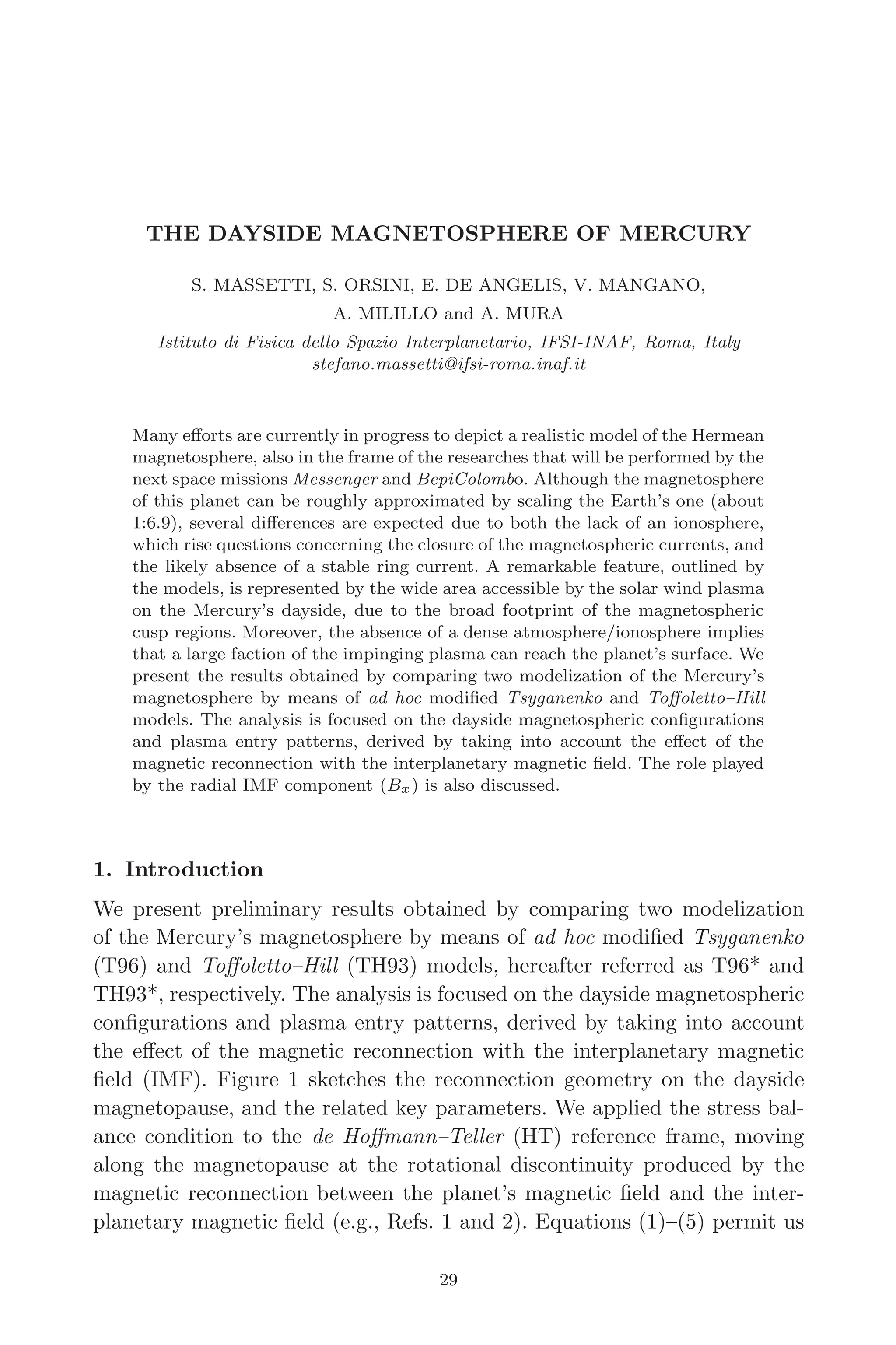
1.
Advanced In GeoscienceVolume 3 Planetary
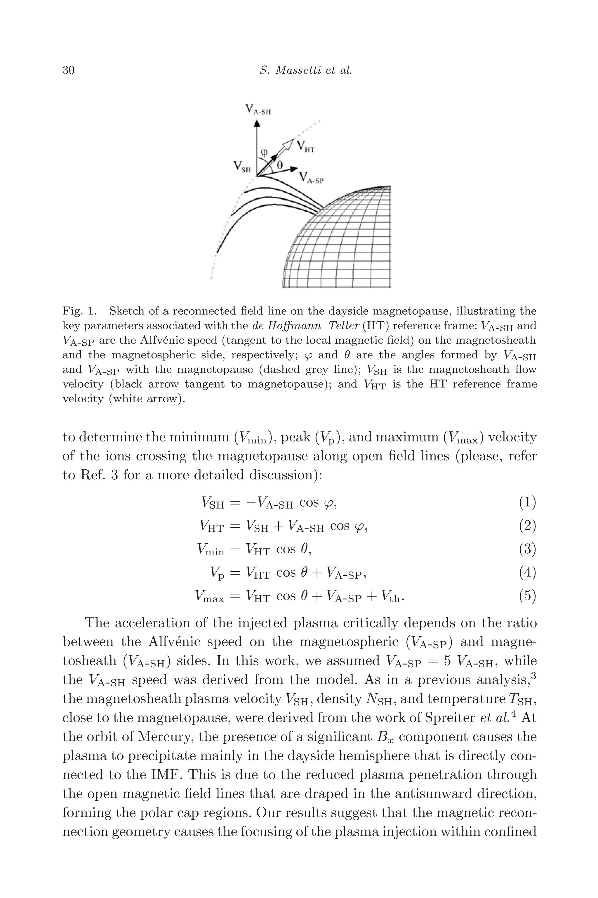
Science Ps Winghuen Ip Editor download
https://ebookbell.com/product/advanced-in-geoscience-
volume-3-planetary-science-ps-winghuen-ip-editor-1002492
Explore and download more ebooks at ebookbell.com
2.
Here are somerecommended products that we believe you will be
interested in. You can click the link to download.
Advances In Geosciences A 4volume Set Volume 29 Hydrological Science
Hs Hydrological Science Hs Kenji Satake Gwofong Lin
https://ebookbell.com/product/advances-in-geosciences-a-4volume-set-
volume-29-hydrological-science-hs-hydrological-science-hs-kenji-
satake-gwofong-lin-51240370
Advances In Geosciences A 4volume Set Volume 31 Solid Earth Science Se
Solid Earth Science Se Kenji Satake Chinghua Lo
https://ebookbell.com/product/advances-in-geosciences-a-4volume-set-
volume-31-solid-earth-science-se-solid-earth-science-se-kenji-satake-
chinghua-lo-51240374
Advances In Geosciences A 4volume Set Volume 28 Atmospheric Science As
And Ocean Science Os Atmospheric Science And Ocean Science Chunchieh
Wu Kenji Satake Jianping Gan
https://ebookbell.com/product/advances-in-geosciences-a-4volume-set-
volume-28-atmospheric-science-as-and-ocean-science-os-atmospheric-
science-and-ocean-science-chunchieh-wu-kenji-satake-jianping-
gan-51240382
Advances In Geosciences A 4volume Set Volume 30 Planetary Science Ps
And Solar Terrestrial Science St Planetary Science Ps And Solar And
Terrestrial Science St Kenji Satake Anil Bhardwaj Andrew Yau
https://ebookbell.com/product/advances-in-geosciences-a-4volume-set-
volume-30-planetary-science-ps-and-solar-terrestrial-science-st-
planetary-science-ps-and-solar-and-terrestrial-science-st-kenji-
satake-anil-bhardwaj-andrew-yau-51240388
3.
Advances In GeosciencesVolume 13 Solid Earth Se Kenji Satake
https://ebookbell.com/product/advances-in-geosciences-volume-13-solid-
earth-se-kenji-satake-2177548
Advances In Geosciences Volume 9 Solid Earth Ocean Science Atmospheric
Science Winghuen Ip
https://ebookbell.com/product/advances-in-geosciences-volume-9-solid-
earth-ocean-science-atmospheric-science-winghuen-ip-2180084
Advances In Geosciences Volume 11 Hydrological Science Hs Namsik Park
https://ebookbell.com/product/advances-in-geosciences-
volume-11-hydrological-science-hs-namsik-park-2181166
Advances In Geosciences Volume 10 Atmospheric Science As Gyan Prakash
Singh
https://ebookbell.com/product/advances-in-geosciences-
volume-10-atmospheric-science-as-gyan-prakash-singh-2198678
Advances In Geosciences Volume 1 Solid Earth Winghuen Ip
https://ebookbell.com/product/advances-in-geosciences-volume-1-solid-
earth-winghuen-ip-5068256
6.
A d va n c e s i n
Geosciences
Volume 3: Planetary Science (PS)
NEW JERSEY •LONDON • SINGAPORE • BEIJING • SHANGHAI • HONG KONG • TAIPEI • CHENNAI
World Scientific
Editor-in-Chief
Wing-Huen Ip
National Central University, Taiwan
Volume Editor-in-Chief
Anil Bhardwaj
Vikram Sarabhai Space Centre, India
A d v a n c e s i n
Geosciences
Volume 3: Planetary Science (PS)
April 7, 200614:12 WSPC/SPI-B368 Advances in Geosciences Vol. 3 fm
EDITORS
Editor-in-Chief: Wing-Huen Ip
Volume 1: Solid Earth (SE)
Editor-in-Chief: Chen Yuntai
Editors: Zhong-Liang Wu
Volume 2: Solar Terrestrial (ST)
Editor-in-Chief: Marc Duldig
Editors: P. K. Manoharan
Andrew W. Yau
Q.-G. Zong
Volume 3: Planetary Science (PS)
Editor-in-Chief: Anil Bhardwaj
Editors: Francois Leblanc
Yasumasa Kasaba
Paul Hartogh
Ingrid Mann
Volume 4: Hydrological Science (HS)
Editor-in-Chief: Namsik Park
Editors: Eiichi Nakakita
Chulsang Yoo
R. B. Singh
Volume 5: Oceans & Atmospheres (OA)
Editor-in-Chief: Hyo Choi
Editors: Milton S. Speer
v
April 7, 200614:12 WSPC/SPI-B368 Advances in Geosciences Vol. 3 fm
REVIEWERS
The Editors of Volume 3 would like to acknowledge the following referees
who have helped review the papers published in this volume:
Mario Acuna
Johannes Benkhoff
R. Binzel
Michel Blanc
Hermann Boehnhardt
E. Bois
Graziella Branduardi-Raymont
Emma J. Bunce
Iver Cairns
Maria Teresa Capria
Alberto Cellino
Michael Collier
Gabriele Cremonese
Alexander Dalgarno
D. Davis
Yoshifumi Futaana
Marina Galand
Mark Gurwell
Walt Harris
Martin Hilchenbach
Takeshi Imamura
Wing -H. Ip
Vlad Izmodenov
Esa Kallio
H. Kawakita
Rosemary Killen
A. S. Kirankumar
Hirtsugu Kojima
Andreas Kopp
Norbert Krupp
Michael Kueppers
Harri Laakso
Rosine Lallement
Yves Langevin
Luisa-M. Lara
E. Pilat Lohinger
Maria J. Lopez-Gonzalez
Bjørn Lybekk
B. Marsden
Philippe Masson
Michael Mendillo
Patrick Michel
Rene Michelsen
T. E. Moore
Thomas. G. Mueller
Alessandro Mura
Masato Nakamura
Rumi Nakamura
Juergen Oberst
Stefano Orsini
Leon Phillips
Jolene Pickett
Brain Ramsey
H. Rishbeth
Yoshifumi Saito
Gerd Sonnemann
Ann Sprague
E. Tedesco
Philippe Thebault
Johan Warell
Richard Wayne
Stuart Weidenschilling
Paul Weissman
O. Witasse
Peter Wurz
Pierre Vernazza
Andrew Yau
vii
April 7, 200614:12 WSPC/SPI-B368 Advances in Geosciences Vol. 3 fm
Contents
Editors v
Reviewers vii
Review of Mariner 10 Observations: Mercury Surface
Impact Processes 1
Clark R. Chapman
Earth Ground-Based Observations of Mercury
Exosphere — Magnetosphere — Surface Relations 5
Leblanc François
On the Dynamics of Charged Particles in
the Magnetosphere of Mercury 17
Dominique C. Delcourt and Kanako Seki
The Dayside Magnetosphere of Mercury 29
S. Massetti, S. Orsini, E. De Angelis, V. Mangano,
A. Milillo and A. Mura
Neutral Atom Emission from Mercury 37
A. Mura, S. Orsini, A. Milillo, D. Delcourt, A. M. Di Lellis,
E. De Angelis and S. Massetti
Bepicolombo — MPO Scientific Aspects and
System Update 51
Johannes Benkhoff and Rita Schulz
Diagnosing the Mercury Plasma Environment Using
Low-Frequency Electric Field Measurements 63
L. G. Blomberg and J. A. Cumnock
ix
15.
April 7, 200614:12 WSPC/SPI-B368 Advances in Geosciences Vol. 3 fm
x Contents
Plasma/Radio Wave Observations at Mercury by the
Bepicolombo MMO Spacecraft 71
H. Matsumoto, J.-L. Bougeret, L. G. Blomberg, H. Kojima,
S. Yagitani, Y. Omura, M. Moncuquet, G. Chanteur, Y. Kasaba,
J.-G. Trotignon, Y. Kasahara and Bepicolombo MMO PWI Team
Low Energy Ion Observation by Mercury Magnetospheric
Orbiter: MMO 85
Yoshifumi Saito, Dominique Delcourt and Andrew Coates
Ice on the Moon and Mercury 93
Dana H. Crider, Rosemary M. Killen and Richard R. Vondrak
Global High-Resolution Stereo Mapping of the Moon
with the Selene Terrain Camera 101
Jun’ichi Haruyama, Makiko Ohtake, Tsuneo Matsunaga
and LISM Working Group
Oxygen Chemistry in the Venus Middle Atmosphere 109
F. P. Mills, M. Sundaram, T. G. Slanger, M. Allen and Y. L. Yung
Observations in the Shadow of Mars by the Neutral
Particle Imager 119
M. Holmström, K. Brinkfeldt, S. Barabash and R. Lundin
Observational Features of the Secondary Layer of the
Martian Ionosphere 135
Hai-Ren Liao, Jing-Song Wang, Hong Zou and
Xiao-Dong Wang
Martian Atmosphere During the 2001 Global Dust Storm:
Observations with SWAS and Simulations with a
General Circulation Model 145
Takeshi Kuroda, Alexander S. Medvedev and Paul Hartogh
The Bulk Density of Cometary Nuclei 155
Björn J. R. Davidsson
Lyman-α Observations of Sungrazing Comets
with the SOHO/UVCS Instrument 171
A. Bemporad, G. Poletto, J. Raymond and S. Giordano
16.
April 7, 200614:12 WSPC/SPI-B368 Advances in Geosciences Vol. 3 fm
Contents xi
An Investigation of the Light Curve of Deep Impact
Target Comet 185
Vitaly Filonenko and Klim Churyumov
Three-Dimensional MHD Simulation of the Solar
Wind Interaction with Comets 191
Mehdi Benna and Paul R. Mahaffy
XMM-Newton Observations of X-Ray Emission
from Jupiter 203
G. Branduardi-Raymont, A. Bhardwaj, R. Elsner, R. Gladstone,
G. Ramsay, P. Rodriguez, R. Soria, H. Waite and T. Cravens
X-Ray Emission from Jupiter, Saturn, and Earth:
A Short Review 215
Anil Bhardwaj
Instrumentation and Observations of the X-Ray
Spectrometer Onboard Hayabusa 231
Tatsuaki Okada, Kei Shirai, Yukio Yamamoto, Takehiko Arai,
Kazunori Ogawa, Kozue Hosono and Manabu Kato
A Mission Called SAPPORO 241
W.-H. Ip, I.-G. Jiang, D. Kinoshita, L. N. Hau, A. Fujiwara,
Y. Saito, F. Yoshida, K. W. Min, Anil Bhardwaj, H. Boehnhardt,
P. Hartogh, T. M. Capria, G. Cremonese, A. Milillo, S. Orisini,
D. Gautier, D. Jewitt and T. Owen
Observation of Luminous Transient Phenomena
on Planetary Bodies 255
Mario Di Martino and Albino Carbognani
Short Electric-Field Antennae as Diagnostic Tools
for Space Plasmas and Ground Permittivity 271
Jean-Gabriel Trotignon
Infrared High-Resolution Spectroscopy of Pluto by
Subaru Telescope 281
Takanori Sasaki, Masateru Ishiguro, Daisuke Kinoshita
and Ryosuke Nakamura
17.
April 7, 200614:12 WSPC/SPI-B368 Advances in Geosciences Vol. 3 fm
xii Contents
Understanding the Origin of the Asteroids Through the
Study of Vesta and Ceres: The Role of Dawn 287
Alberto Cellino, Fabrizio Capaccioni, Maria Teresa Capria,
Angioletta Coradini, Maria Cristina De Sanctis,
Horst U. Keller, Thomas H. Prettyman, Carol A. Raymond
and Christopher T. Russell
The Expected Role of Gaia For Asteroid Science 299
Alberto Cellino, Aldo Dell’oro and Paolo Tanga
Lightcurves of the Karin Family Asteroids 317
Takashi Ito and Fumi Yoshida
Difference in Degree of Space Weathering on Newborn
Asteroid Karin 331
Takanori Sasaki, Sho Sasaki, Jun-Ichi Watanabe,
Tomohiko Sekiguchi, Fumi Yoshida, Takashi Ito,
Hideyo Kawakita, Tetsuharu Fuse, Naruhisa Takato
and Budi Dermawan
Size Distribution of Asteroids and Old Terrestrial Craters:
Implications for Asteroidal Dynamics During LHB 337
Takashi Ito, Robert G. Strom, Renu Malhotra, Fumi Yoshida
and David A. Kring
Status of the TAOS Project and a Simulator for
TNO Occultation 345
Sun-Kun King, Charles Alcock, Tim Axelrod, Federica B. Bianco,
Yong-Ik Byun, Wen-Ping Chen, Kem H. Cook, Yung-Hsin Chang,
Rahul Dave, Joseph Giammarco, Typhoon Lee, Matthew Lehner,
Jack Lissauer, Stuart Marshall, Soumen Mondal, Imke De Pater,
Rodin Porrata, John Rice, Megan E. Schwamb, Andrew Wang,
Shiang-Yu Wang, Chih-Yi Wen and Zhi-Wei Zhang
Neo-Survey and Hazard Evaluation 359
Yuehua Ma and Guangyu Li
ENA Signals Coming from the Heliospheric Boundaries 367
K. C. Hsieh
18.
April 7, 200614:12 WSPC/SPI-B368 Advances in Geosciences Vol. 3 fm
Contents xiii
Habitable Zones for Earth-Like Planets in the 47 UMa
Planetary System 377
Jianghui Ji and Lin Liu
JAXA Future Program for Solar System Sciences 389
Masato Nakamura, Manabu Kato and Yasumasa Kasaba
March 16, 200613:47 WSPC/SPI-B368 Advances in Geosciences Vol. 3 ch01
REVIEW OF MARINER 10 OBSERVATIONS: MERCURY
SURFACE IMPACT PROCESSES
CLARK R. CHAPMAN
Southwest Research Institute, 1050 Walnut Street
Suite 400, Boulder, CO 80302, USA
cchapman@boulder.swri.edu
The major evidence concerning Mercury’s craters remains the imaging of
Mariner 10 from over three decades ago. We are beginning to gain information
about Mercury’s unimaged side from Earth-based radar. The MESSENGER
mission will start making major advances in a few years. Issues that have devel-
oped and remain to be resolved include the specific roles of the Late Heavy
Bombardment and of hypothetical “vulcanoids” in cratering the planet, which
affect calibration of the absolute chronology of Mercury’s geological and geo-
physical evolution, and the role of secondary cratering, by ejecta from both the
visible craters and from the numerous large basins.
1. Introduction
Mercury’s surface was first revealed by Mariner 10 imaging. Generally,
Mercury is heavily cratered, with less cratered regions, superficially sim-
ilar to the Moon. Craters range from nearly saturated small-sized craters
(many show clustering suggestive of secondaries) up to enormous multi-
ringed basins, of which Caloris is the most prominent in Mariner 10 images.
Dozens of basins have been tentatively identified. Morphometric statistics
of Mercury’s craters have been compared with those for other terrestrial
bodies and interpreted in terms of differences in surface gravity and other
factors.1–4
Craters are used for both relative and absolute age-dating of geologi-
cal units on planetary bodies. Early interpretations of Mercury’s cratering
record drew analogies from the Moon: it was supposed that most craters
and basins formed about 3.9 Ga, during the same Late Heavy Bombardment
(LHB) that dominated lunar cratering.5
Through superposition relation-
ships with other geological features (e.g., lobate scarps), a tentative chronol-
ogy for Mercury’s geological history was derived (tied to the old Tolstoj
basin and the younger Caloris basin), raising potential incompatibilities
1
21.
March 16, 200613:47 WSPC/SPI-B368 Advances in Geosciences Vol. 3 ch01
2 C. R. Chapman
with geophysical inferences about interior cooling rates and processes that
generate Mercury’s magnetic field.2,5
Craters on Mercury (and other bodies) are studied in several ways.
Beyond the Mariner 10 imaging, and expected imaging from MESSENGER
and BepiColombo missions to Mercury, radar delay-doppler mapping, some
at better than 2 km resolution, from Arecibo6
and other radar telescopes is
starting to rival the resolution of the global-scale Mariner 10 imaging. Stud-
ies comparing Mercury’s crater population with those on the Moon, Mars,
and other bodies provides useful understanding. Also relevant is modeling
of impactor populations and simulations of their impact history on Mer-
cury. Theoretical studies of cratering mechanics, ejecta distributions, and
regolith evolution have sometimes been applied to Mercury.
In detail, Mercury’s craters have morphological differences from those
on the Moon and Mars, partly due to differences in gravity and impactor
environment (e.g., higher velocity impacts on Mercury), but most of the
differences are probably due to the different geological processes that erode
and degrade craters after they have formed on the various planets. For
example, while many craters on Mars extend back to the Late Heavy Bom-
bardment epoch that may be contemporaneous with the formation of many
of Mercury’s craters, the Martian surface has undergone glaciation, rain-
fall/runoff, dust storms, sedimentation, exhumation, and many other pro-
cesses not thought likely to have been relevant on Mercury.
2. Origins of Mercury’s Craters
Potential sources for the impactors that formed Mercury’s craters are
numerous. In principle, the size distributions and the impact rates could
have varied with time and in ways not necessarily correlated with the crater-
ing histories of other bodies. Sources include: the near-Earth asteroids and
their cousins (of which only three have yet been found) that orbit entirely
interior to Earth’s orbit (termed Apoheles); short- and long-period comets,
including sun-grazers; vulcanoids, an as-yet-undiscovered hypothetical pop-
ulation of remnant planetesimals from accretionary epochs, orbiting mainly
inside Mercury’s orbit; and secondary cratering by ejecta from basins and
large primary craters. Endogenic crater-forming processes (e.g., volcanism)
are also possible. Differences in asteroid/comet cratering rates (perhaps
including the LHB) are not expected to vary by large factors for Mer-
cury compared with the Earth–Moon system or Mars. But if vulcanoids
were/are important, they could have extended the duration of Mercury’s
22.
March 16, 200613:47 WSPC/SPI-B368 Advances in Geosciences Vol. 3 ch01
Review of Mariner 10 Observations: Mercury Surface Impact Processes 3
intense cratering into epochs far later than the LHB, and even overprinted
the LHB.7
It is possible that planetesimals interior to Mercury’s orbit never formed
or that they were destroyed (e.g., by their mutual, high-velocity collisions)
before the epoch of the LHB. But if they did survive such early pro-
cesses, it appears that their subsequent depletion by Yarkovsky effect drift
might have lasted for several billion years, perhaps resulting in appreciable
post-LHB cratering of Mercury.8
(The Yarkovsky effect has been found to
have a potent effect in changing the orbits of small solar system bodies;
it acts on rotating bodies due to the asymmetry between insolation and
re-radiation in the thermal infrared.) The point here is not to assert that
current assumptions that tie Mercury’s absolute geological chronology to
the LHB are wrong, but that such a chronology should not be taken as a
strong constraint. There are other geophysical aspects of Mercury that were
surprising to the Mariner 10 researchers and originally seemed difficult to
reconcile. Mercury appears to have an active dynamo-generated magnetic
field, although this has been debated. Mercury’s buckled crust (expressed as
a global distribution of lobate scarps) suggests global cooling and shrinking
in post heavy-cratering epochs, but perhaps the cooling and crustal short-
ening has not gone to completion. Recent bistatic radar interferometric
studies9
suggest the presence of a molten layer within Mercury. Theoreti-
cal modeling combined with hypotheses concerning impurities in the core
may have reconciled Mercury’s small size and rapid cooling rate with these
indications of a still molten portion of the planet’s core. Nevertheless, the
evaluation of these geophysical issues should not be strongly constrained
by any particular cratering chronology. Mercury’s heavily cratered regions
may, in fact, reflect LHB cratering and its internal geological processes may
have shut down soon afterwards (access to molten magma may have been
closed off by crustal compression). Alternatively, both the cratering and the
faulting could have extended billions of years closer to the present time, if
vulcanoid cratering was important.
3. Secondary Cratering
Secondary cratering may be a much more important process than previously
thought. Studies of both the sparsely cratered surface of Europa10
and of
Mars11
have recently suggested that the steep branch of the crater size-
frequency relation for craters smaller than a few km (originally identified by
Shoemaker12
as the “secondary” branch but later attributed to the inherent
23.
March 16, 200613:47 WSPC/SPI-B368 Advances in Geosciences Vol. 3 ch01
4 C. R. Chapman
size-distribution of collisionally evolved asteroids) really is dominated by
secondaries from primaries larger than 10 km. One study, for example, finds
that a single 10 km diameter crater on Mars may be responsible for as
many as a billion secondary craters larger than 10 m diameter.11
Crater
chains, crater rays, and clusters of small craters visible in Mariner 10 images
were already attributed to the process of secondary cratering on Mercury.
The global high-resolution imaging expected from MESSENGER, combined
with the extensive intercrater plains on Mercury as well as the tendency for
ejecta on Mercury to be less widely distributed around the globe than is
true for the Moon, all should help explicate the role of secondary cratering
as a planetary process. Possibly, many supposed primary craters several
tens of km in size may instead be secondaries from basin-forming impacts,
as Wilhelms13
believes is true for the Moon.
References
1. F. Vilas, C. R. Chapman and M. S. Matthews, eds., Mercury (University of
Arizona Press, Tucson, 1988).
2. P. D. Spudis and J. E. Guest, in Mercury, eds. F. Vilas, C. R. Chapman and
M. S. Matthews (University of Arizona Press, Tucson, 1988), p. 118.
3. R. J. Pike, in Mercury, eds. F. Vilas, C. R. Chapman and M. S. Matthews
(University of Arizona Press, Tucson, 1988), p. 165.
4. P. H. Schultz, in Mercury, eds. F. Vilas, C. R. Chapman and M. S. Matthews
(University of Arizona Press, Tucson, 1988) p. 274.
5. R. G. Strom and G. Neukum, in Mercury, eds. F. Vilas, C. R. Chapman and
M. S. Matthews (University of Arizona Press, Tucson, 1988), p. 336.
6. J. K. Harmon, P. J. Perillat and M. A. Slade, Icarus 149 (2001) 1.
7. M. A. Leake, C. R. Chapman, S. J. Weidenschilling, D. R. Davis and
R. Greenberg, Icarus 71 (1987) 350.
8. D. Vokrouhlichy, P. Farinella and W. F. Bottke, Icarus 148 (2000) 147.
9. J. L. Margot, S. J. Peale, R. F. Jurgens, M. A. Slade and I. V. Holin,
Proccedings of the 35th COSPAR (2004), p. 3693.
10. E. B. Bierhaus, C. R. Chapman and W. J. Merline, Nature, 437, doi:10.1038/
nature 04069 (October 2005) 1125–1127.
11. A. S. McEwen et al., Icarus 176 (2005) 351.
12. E. M. Shoemaker, in Ranger VII Pt. II. Experimenters’ Analyses and Inter-
pretations, eds. R. L. Heacock et al. (JPL Tech. Rept. No. 32-700, 1965), p. 75.
13. D. E. Wilhelms, Lunar and Planetary Sci. Conf. 7th (1976), p. 2883.
24.
March 16, 200613:47 WSPC/SPI-B368 Advances in Geosciences Vol. 3 ch02
EARTH GROUND-BASED OBSERVATIONS OF MERCURY
EXOSPHERE — MAGNETOSPHERE — SURFACE
RELATIONS
LEBLANC FRANÇOIS
Service d’Aéronomie du CNRS/IPSL, France
francois.leblanc@aerov.jussieu.fr
Mariner-10 flybys of Mercury were the main sources of information on Mer-
cury’s exosphere up to the discovery of the exospheric sodium emission from
ground based observatories (Potter and Morgan, Science 229 (1985) 651–653).
These later observations were followed by the discovery of potassium (Potter
and Morgan, Icarus 67 (1986) 336–340) and calcium emissions in Mercury’s
exosphere (Bida et al., Nature 404 (2000) 159–161). Several ground-based
observations have underlined the significant spatial and temporal variations
of Mercury’s exosphere. Such observations lead to the suggestion of a large
number of potential sources of ejection of volatiles from Mercury’s surface, but
also to the suggestions of strong relations between Mercury’s exosphere and its
magnetosphere as well as between Mercury’s exosphere and upper surface.
1. Introduction
Since the Mariner-10 flybys of Mercury, most of the studies and obser-
vations of Mercury’s neutral exosphere have concerned the bright sodium
exospheric emissions.1–3
Since its first observation,4
several observations
underlined the significant spatial and temporal variabilities of Mercury’s
sodium exosphere.5,6
Such observations lead to the suggestion of a large
number of potential sources of ejection of the sodium atoms from Mer-
cury’s surface. They also suggest strong relations between Mercury’s exo-
sphere and its magnetosphere7
as well as between Mercury’s exosphere and
upper surface.8–10
This paper is focused on the different sources of variation of the known
exospheric abundances and does not intend to be a complete review on
Mercury’s exosphere already done in several recent papers.1–3
Most of
these variations derived from the strong links between Mercury’s exosphere,
its magnetosphere, and its upper surface. These exospheric variations can
therefore, be also interpreted as indirect observations of the characteristics
of the magnetosphere and of the upper surface. This paper emphasizes the
5
25.
March 16, 200613:47 WSPC/SPI-B368 Advances in Geosciences Vol. 3 ch02
6 F. Leblanc
most debated and recent questions and the key information that may be
derived from ground-based observations, on Mercury’s exosphere — magne-
tosphere — upper surface system. Such information is particularly needed
in preparation of the forthcoming Messenger and BepiColombo missions.
In Sec. 2, we give a brief overview of the known neutral and ion compo-
sitions of Mercury’s exosphere. Section 3 describes some important sources
of variations of the exospheric abundance related to the coupling between
Mercury’s exosphere, its upper surface, and its magnetosphere. Section 4
concludes this paper.
2. Exospheric Composition
The only few elements that Mariner-10 provided on Mercury’s neutral exo-
sphere are:
(i) the measurements of H and He with surface density of 250 H/cm3
and
6 × 10³
He/cm3
,11
(ii) an identification of O column density with suggested value for its sur-
face density of 4.4 × 10⁴
O/cm3
,12,13
(iii) an upper limit for the total content of the exosphere at the subso-
lar point: 107
neutral particles/cm3
from the solar occultation UV
measurement.12
Ground-based observations identified:
(i) Na atoms with zenith sub-solar column density of 1011
Na/cm2
,4,14
(ii) K atoms with column density of 109
K/cm2
,4,15,16
(iii) Ca atoms with column density of 108
Ca/cm2
.17
Only upper limits are known for other elements from Mariner-10 solar
occultation UV experiment: at the surface density 1.4 × 10⁷
H2/cm3
, 2.5 ×
107
O2/cm3
, 2.3 × 10⁷
N2/cm3
, 1.5 × 10⁷
H2O/cm3
, 1.6 × 10⁷
CO2/cm3
and
3.1×10⁷
Ar/cm3
.12
Hunten et al.11
suggested that densities of 104
H2/cm3
,
1 H2O/cm3
, and 1 CH4/cm3
are more realistic for these species (for H2O
and CH4 in particular because of a short-lifetime against photoionization).
At the Moon, which is the best analog of Mercury’s exosphere, O2 has
never been measured, N2 has been measured with 8 × 10²
N2/cm3
, CO2
with 103
CO2/cm3
(the same density as for CO), and Ar with 4 × 10⁴
to 105
Ar/cm3
.18
Upper limits at the Moon for O, N, C, Fe, and S
below 103
particles/cm3
, Si and Al below 102
particles/cm3
have also been
reported.18
26.
March 16, 200613:47 WSPC/SPI-B368 Advances in Geosciences Vol. 3 ch02
Mercury’s Exosphere — Magnetosphere — Surface Relations 7
There are only two published works providing some estimates of the
abundances of other non-identified elements.19,20
Only a measurement of Mercury’s electron density has been performed
by Mariner-10 radio occultation experiment.21
These authors reported
an upper limit for the electron density of 103
electrons/cm3
. This is
probably why, up to now, very few studies on the ion exosphere have
been published.22–26
However, the ion exosphere has been widely quoted
to play.
(i) A crucial role for the neutral exosphere first of all as the product of its
ionization11
but also as agent for sputtering of the surface.27
Planetary
ions are not only at the origin of one mechanism producing the neu-
tral exosphere but also a significant source of enrichment of the upper
surface from which the neutral exosphere is formed.15,28
(ii) Ions are also seen as a larger source of loss for Mercury’s exosphere
through solar wind entrainment rather than direct neutral loss.
The ion exosphere is fully unknown but simple calculations based on
photo ionization of the neutral component can be done to infer what could
be the main ion species in Mercury’s exosphere.24,29
3. Sources of Variation of Mercury’s Exosphere Content
The exospheric column and surface densities given in the previous section
should be also considered with regard to all the sources of temporal and
spatial variations of Mercury’s exosphere that is as follows:
(i) Mercury’s orbit around the Sun induces changes in the average solar
flux by a factor 2.3 but also an irregular apparent motion of the Sun
as seen from Mercury,
(ii) Short and long-term variations of the solar wind should significantly
change Mercury’s magnetosphere, and as a consequence its exosphere,
through changes of solar wind sputtering rate. Coronal mass ejection or
flare events could compress Mercury’s magnetosphere up to its surface
or open large regions to the solar wind. Magnetospheric recycling of
planetary ions could also significantly influence Mercury’s exospheric
content and spatial distribution,
(iii) Mercury’s upper surface content in volatiles is most probably non-
uniform due to the preferential migration of the volatiles into regions
less submitted to sputtering, desorption or vaporization (like nightside
27.
March 16, 200613:47 WSPC/SPI-B368 Advances in Geosciences Vol. 3 ch02
8 F. Leblanc
regions or the parts of high-latitude craters permanently in the
shadow). Such non-uniformity could lead to a non-uniform spatial exo-
spheric distribution.
3.1. Variation due to Mercury’s orbit
Mercury’s eccentricity (0.2056) is the largest of the inner planets of the
solar system. The variation of the heliocentric distance from perihelion
(0.306 AU) to aphelion (0.466 AU) implies a variation of the average inten-
sity of the solar wind and photon fluxes by a factor 2.3. Therefore, solar
wind sputtering, photon-stimulated desorption or photon ionization will
change in efficiency by such a factor in an average (also the brightness of
Mercury’s exosphere as seen from the Earth). Variation of the solar UV flux
and of the solar wind flux on short-time scale is also an important cause of
variability in the exosphere (see as an example the increase of the UV flux
displayed Plate 6 of Ref. 7 and Sec. 3.2.1).
As a consequence, Mercury’s surface temperature also changes signifi-
cantly from a maximum temperature around 650 K at perihelion down to
a maximum temperature around 550 K at aphelion.30
Thermal desorption
and the average energy of the ejected particles by this latter mechanism
will also significantly change along Mercury’s year.
Mercury rotates around the Sun in a 2–3 resonance between orbit
(87.97 Earth days) and sidereal rotation (58.6 Earth days), its diurnal period
being therefore of 176 Earth days.31
This motion leads to an irregular appar-
ent motion of the Sun as seen from Mercury’s surface, in particular, a slow-
ing down and subsequent reversal of the Sun’s apparent motion during a
short period equivalent to few Earth days at perihelion. The Sun’s apparent
motion at Mercury is faster at aphelion. This 2–3 resonance produces hot
and cold longitudes, which correspond to regions of Mercury’s surface that
receive maxima and minima of solar flux along Mercury’s year.32
It also
implies that Mercury’s nightside surface enriched in volatiles (see Sec. 3.3.1
for further explanations), moves into the dayside with a much larger speed
at aphelion than at perihelion. As a consequence, the quantity of volatiles
available for ejection into Mercury’s exosphere is larger at aphelion than at
perihelion, and therefore, Mercury’s total exospheric content may be larger
at aphelion than at perihelion, a trend that seems to be confirmed by the
now extended set of observation of Mercury’s sodium exosphere.9,10,14
In
particular, Killen et al.10
have shown by compiling a large set of observa-
tions of Mercury’s sodium exosphere that Mercury’s sodium exosphere total
28.
March 16, 200613:47 WSPC/SPI-B368 Advances in Geosciences Vol. 3 ch02
Mercury’s Exosphere — Magnetosphere — Surface Relations 9
content might be up to 2.5 times larger at aphelion than at perihelion. A
model which would not consider a variation of the surface content in Mer-
cury’s surface would have predicted a global denser exosphere at perihelion
than at aphelion (up to a factor 2.3) because all processes ejecting sodium
atoms into Mercury’s exosphere are in an average 2.3 more efficient at per-
ihelion than at aphelion. The only way that may compensate this effect
(and actually to invert it in order to be consistent with Killen et al.10
) is to
decrease such an efficiency. A decrease of the available reservoir for ejection
from aphelion to perihelion is the only mechanism up to now that has been
suggested to explain this loss of efficiency.9
3.2. Magnetosphere–exosphere relations
3.2.1. Solar wind penetration
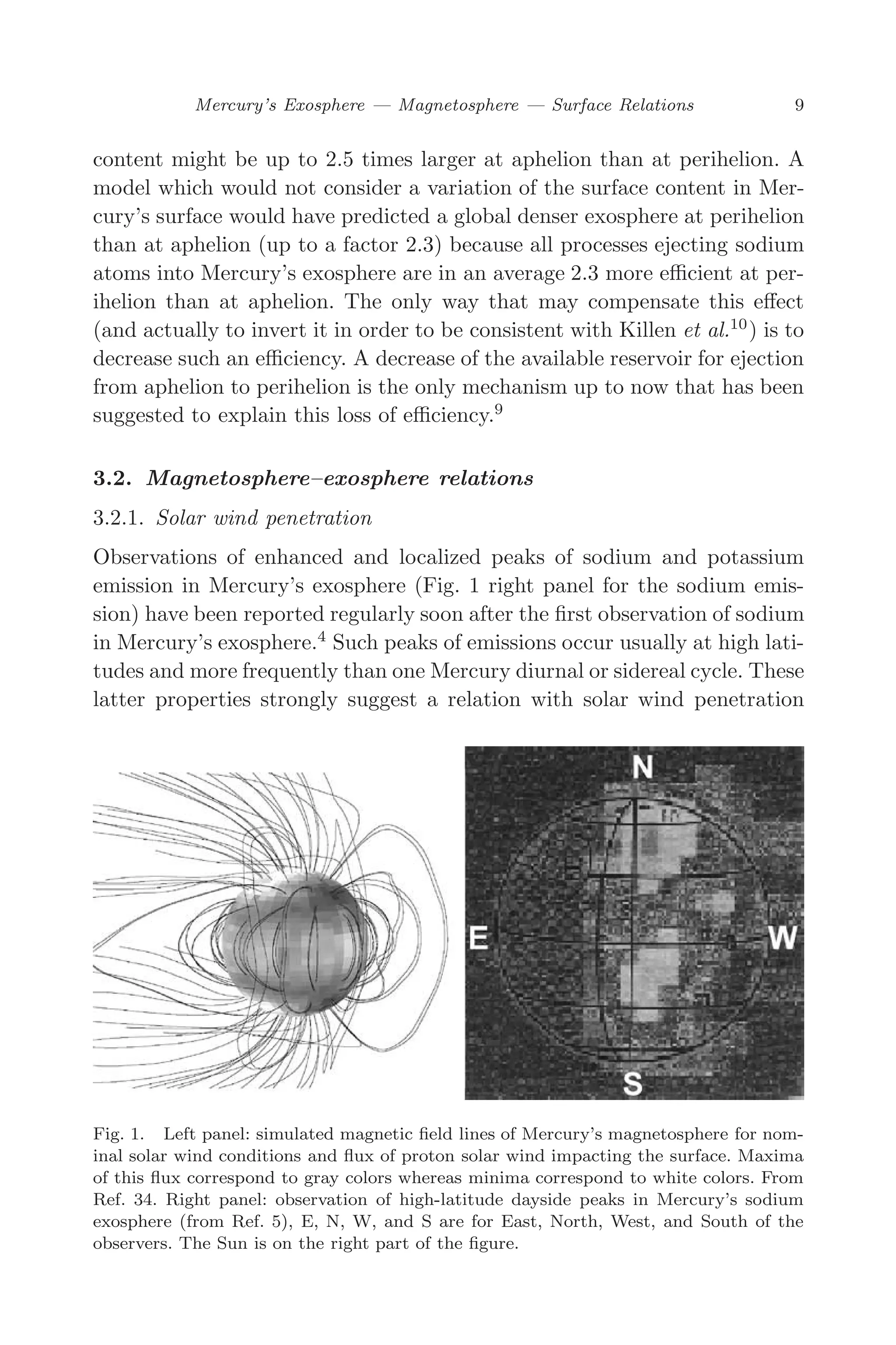
Observations of enhanced and localized peaks of sodium and potassium
emission in Mercury’s exosphere (Fig. 1 right panel for the sodium emis-
sion) have been reported regularly soon after the first observation of sodium
in Mercury’s exosphere.4
Such peaks of emissions occur usually at high lati-
tudes and more frequently than one Mercury diurnal or sidereal cycle. These
latter properties strongly suggest a relation with solar wind penetration
Fig. 1. Left panel: simulated magnetic field lines of Mercury’s magnetosphere for nom-
inal solar wind conditions and flux of proton solar wind impacting the surface. Maxima
of this flux correspond to gray colors whereas minima correspond to white colors. From
Ref. 34. Right panel: observation of high-latitude dayside peaks in Mercury’s sodium
exosphere (from Ref. 5), E, N, W, and S are for East, North, West, and South of the
observers. The Sun is on the right part of the figure.
29.
March 16, 200613:47 WSPC/SPI-B368 Advances in Geosciences Vol. 3 ch02
10 F. Leblanc
of Mercury’s magnetosphere (Fig. 1 left panel) and subsequent sputtering
of the surface by energetic incident solar protons leading to ejection of a
significant number of volatiles such that they can be seen from the Earth
ground-based observatories.5
Solar wind sputtering is in particular an ener-
getic process of ejection and is therefore, able to eject refractory species
into Mercury’s exosphere. Therefore, such refractory species, like calcium,
should be found preferentially above the surface submitted to solar wind
sputtering.5,17
As a matter of fact, the first observations of the calcium
in Mercury’s exosphere reported brighter emissions at high latitudes than
at the equator.17
However, it has been recently suggested after analyzing
4 years of observations, that the origin of the observed exospheric calcium
atoms is preferentially formed by micrometeoroid ejection as molecule and
subsequent photodissociation.33
3.2.2. Solar event encounter
The encounter of a solar event with Mercury could lead to a significant
enhancement of the incident dynamic pressure, such that the dayside mag-
netosphere is no longer able to efficiently shield Mercury’s surface from the
incident solar wind and energetic particles.34,35
Potter et al.36
suggested
a relationship between the observation of a global and rapid increase of
the total content of Mercury’s sodium exosphere and the occurrence of
Mercury-directed Coronal Mass Ejections observed by the SOHO space-
craft coronagraphs. Leblanc et al.37
used a sample energetic particle event
observed at Earth to estimate some of the effects of such an event on the sur-
face sputtering contribution to Mercury’s sodium exosphere. These authors
concluded that fluxes several orders of magnitude larger would be required
to produce Potter et al.’s36
inferred sodium enhancements. Such events are
fully within the range of variation of known solar energetic particle events.
3.2.3. Magnetospheric recycling
Delcourt et al.26
found that planetary Na+
ions may convect to the night-
side, be accelerated and then hit the surface in a non-uniform way.29,38
This
feature is confirmed by hybrid simulations of ion circulation at Mercury.34
Leblanc et al.28
concluded that less than 15% of the photoion reimpact
Mercury’s surface. These authors using typical solar wind conditions found
that enhancement in the Na emissions could be correlated to these bands
of re-implantation. They also suggested that any change in the solar wind
30.
March 16, 200613:47 WSPC/SPI-B368 Advances in Geosciences Vol. 3 ch02
Mercury’s Exosphere — Magnetosphere — Surface Relations 11
conditions could change the magnetospheric structure39
and induce signif-
icant changes in the recycling of magnetospheric ions inducing correlated
variation in the neutral exosphere. Using different neutral exospheric and
magnetospheric models, Killen et al.10
found that between 45 and 65% of
the photoions reimpact the surface, most on the dayside and underlined the
significant role of the electric field of convection in the global dawn to dusk
balance of the recycled ion.
3.3. Upper surface–exosphere relations
3.3.1. Migration of the volatiles
A particle ejected from Mercury’s dayside not on an escaping trajectory
(that is with less than ∼0.1 eV/amu when ejected) will randomly hop and
become temporally absorbed (as example for most of the sodium atoms) or
partially energetically accommodated in Mercury’s upper surface at each
hop (as example for most of the hydrogen and helium atoms).40
Due to
the very high temperature of Mercury’s dayside surface (more than 400 K
during most of the day, see Fig. 2), the period during which such a particle
is absorbed in Mercury’s upper surface is shorter than few Earth minutes
or few Mercury’s seconds (values valid in the case of a sodium atom using
recent laboratory measurements41
and including porosity effect9
). There-
fore, the time needed for such a particle to encounter a cold surface where
it can be trapped for a long period (with respect to Mercury’s day) will be
much shorter than Mercury’s hour. These cold regions are essentially late
evening, early morning or high-latitude regions. This migration of volatiles
into cold regions should lead to a global larger density of trapped volatiles
on the nightside than on the dayside.9
An immediate consequence is a sig-
nificant morning/evening asymmetries of Mercury’s exosphere because of
the release of trapped nightside volatiles at morning. Such morning/evening
asymmetry in the case of Mercury’s sodium exosphere has been discussed
for a long-time up to its recent and unambiguous observation.42
Another putative consequence of this preferential migration of ejected
volatiles into cold surfaces could be the enrichment of Mercury’s surface at
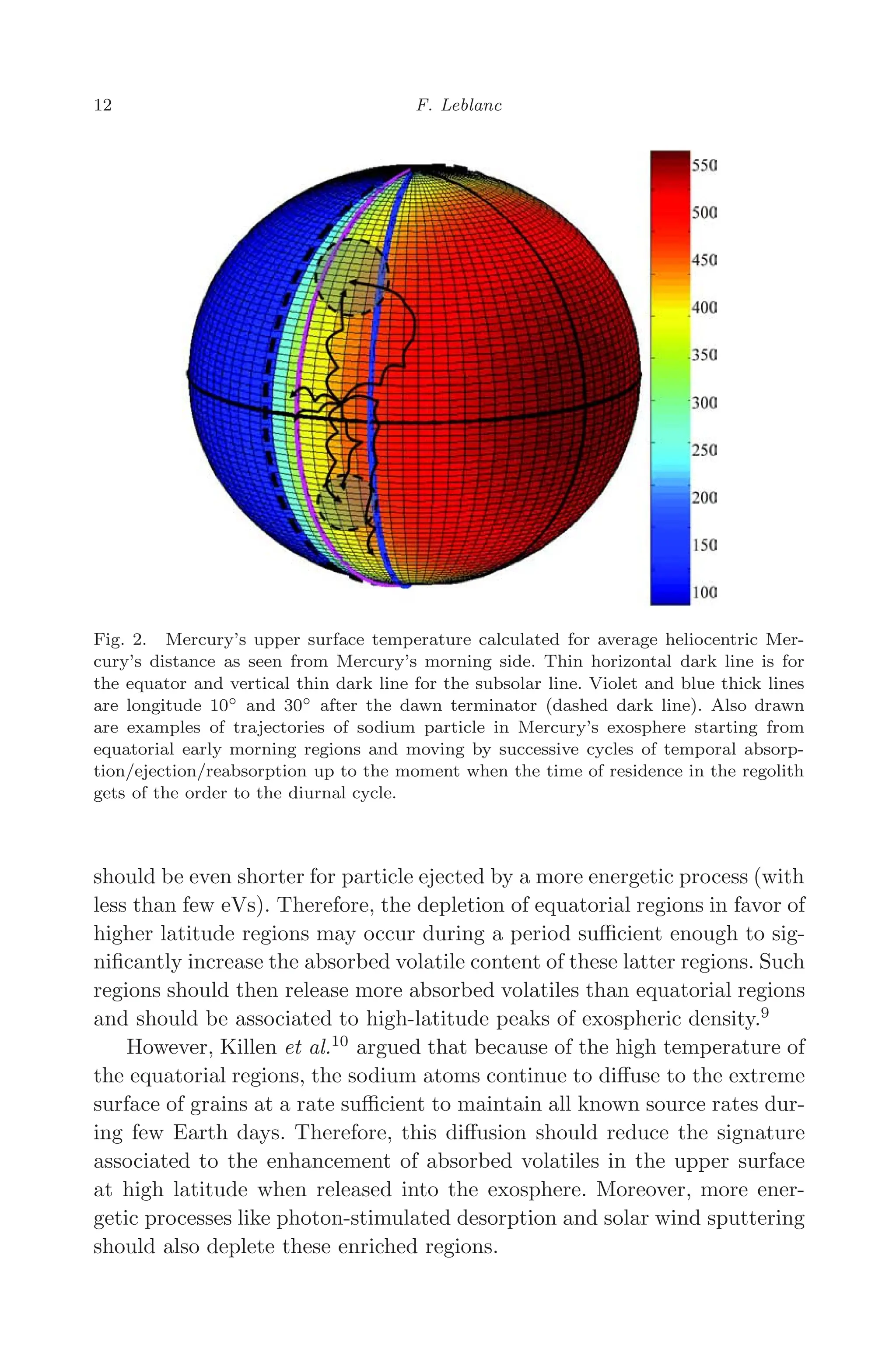
high-latitude early morning. Indeed as illustrated in Fig. 2, in the morn-
ing, equatorial regions get hotter earlier by few degrees in longitude than
high-latitude regions. As an example, 60◦
latitude regions reach equatorial
surface temperature few tens of Earth hours later. Such a period is roughly
the time for a thermally desorbed particle (with less than 0.06 eV when
ejected) to move by a distance of the order of Mercury radius. Such a time
31.
March 16, 200613:47 WSPC/SPI-B368 Advances in Geosciences Vol. 3 ch02
12 F. Leblanc
Fig. 2. Mercury’s upper surface temperature calculated for average heliocentric Mer-
cury’s distance as seen from Mercury’s morning side. Thin horizontal dark line is for
the equator and vertical thin dark line for the subsolar line. Violet and blue thick lines
are longitude 10◦ and 30◦ after the dawn terminator (dashed dark line). Also drawn
are examples of trajectories of sodium particle in Mercury’s exosphere starting from
equatorial early morning regions and moving by successive cycles of temporal absorp-
tion/ejection/reabsorption up to the moment when the time of residence in the regolith
gets of the order to the diurnal cycle.
should be even shorter for particle ejected by a more energetic process (with
less than few eVs). Therefore, the depletion of equatorial regions in favor of
higher latitude regions may occur during a period sufficient enough to sig-
nificantly increase the absorbed volatile content of these latter regions. Such
regions should then release more absorbed volatiles than equatorial regions
and should be associated to high-latitude peaks of exospheric density.9
However, Killen et al.10
argued that because of the high temperature of
the equatorial regions, the sodium atoms continue to diffuse to the extreme
surface of grains at a rate sufficient to maintain all known source rates dur-
ing few Earth days. Therefore, this diffusion should reduce the signature
associated to the enhancement of absorbed volatiles in the upper surface
at high latitude when released into the exosphere. Moreover, more ener-
getic processes like photon-stimulated desorption and solar wind sputtering
should also deplete these enriched regions.
32.
March 16, 200613:47 WSPC/SPI-B368 Advances in Geosciences Vol. 3 ch02
Mercury’s Exosphere — Magnetosphere — Surface Relations 13
3.3.2. Topography effects
Another relation between upper surface and exosphere is related to the
presence of large craters and basins at Mercury’s surface. In particular,
Sprague43
suggested relation between the presence in Mercury’s morning
of Caloris basin, a crater with a diameter equal to half-Mercury’s radius,
and an apparent increase in Mercury’s potassium total content. In the same
way, Potter et al.36
observed a three times enhancement of Mercury’s total
sodium content when Caloris basin was in Mercury’s early morning. Such
type of large topographic anomalies at Mercury’s surface as well as smaller
craters14
could therefore, have an important role in supplying Mercury’s
exosphere in volatiles.44
4. Conclusions
Up to now, only few elements of Mercury’s exosphere have been identified,
most probably representing only few percents of the total content of the
exosphere. Moreover, the influences of Mercury’s magnetosphere and of
Mercury’s surface composition are key points to be solved in order to fully
understand the origin, dynamic, and composition of Mercury’s exosphere.
Any description of Mercury’s exosphere has then to consider the numer-
ous sources of variation which are:
(i) The changes along Mercury’s orbit of the different mechanisms of pro-
duction, destruction, and recycling.
(ii) The role of the solar wind and photon flux and their short and long-
times variations.
(iii) The changes of Mercury’s magnetosphere with respect to the inter-
planetary magnetic field and also possible encounters with solar event.
(iv) The role of large and small topographic structures at Mercury’s
surface.
Very little has been said in this paper about the different mechanisms
of ejection from the surface thought to be at work at Mercury.7,45
Actually,
the way each species is ejected from Mercury’s upper surface defines their
initial energy and therefore, their spatial distribution. Spatial variations
also depend on the regions of Mercury’s surface where such species are pro-
duced and the variations of the ejected flux intensity with respect to solar
conditions, to distance to the Sun and to position on Mercury’s surface.
At the end, the solar radiation pressure has been suggested to model
the shape of Mercury’s exosphere for some species.46
In particular, it has
33.
March 16, 200613:47 WSPC/SPI-B368 Advances in Geosciences Vol. 3 ch02
14 F. Leblanc
been suggested that Mercury’s exospheric sodium tail recently observed47
is
essentially shaped by the solar pressure acting on the sodium atoms ejected
from Mercury’s surface.9
References
1. R. M. Killen and W.-H. Ip, Rev. Geophys. 37 (1999) 361–406.
2. F. Leblanc, E. Chassefière, R. E. Johnson, D. M. Hunten, E. Kallio,
D. C. Delcourt, R. M. Killen, J. G. Luhmann, A. E. Potter, A. Jambon,
G. Cremonese, M. Mendillo, N. Yan and A. L. Sprague, Submitted to Plan-
etary Space Science (2006).
3. A. Milillo, P. Wurz, S. Orsini, D. Delcourt, E. Kallio, R. M. Killen,
H. Lammer, S. Massetti, A. Mura, S. Barabash, G. Cremonese, I. A. Daglis,
E. De Angelis, A. M. Di Lellis, S. Livi, V. Mangano and K. Torkar, Space
Sci. Rev. 117 (2005) 397–443.
4. A. E. Potter and T. H. Morgan, Science 229 (1985) 651–653.
5. A. E. Potter and T. H. Morgan, Science 248 (1990) 835.
6. A. E. Potter, T. H. Morgan and R. M. Killen, Plan. Space Sci. 47 (1999)
1441–1448.
7. R. M. Killen, A. E. Potter, P. Reiff, M. Sarantos, B. V. Jackson, P. Hick and
B. Giles, J. Geophys. Res. 106, (2001) 20,509–20,525.
8. D. M. Hunten and A. L. Sprague, Adv. Space Res. 19 (1997) 1551–1560.
9. F. Leblanc and R. E. Johnson, Icarus 164 (2003) 261–281.
10. R. M. Killen, M. Sarantos, A. E. Potter and P. H. Reiff, Icarus 171
(2004) 1–19.
11. D. M. Hunten, T. M. Morgan and D. M. Shemansky, The Mercury atmo-
sphere, in Mercury, eds. F. Vilas, C. Chapman and M. Matthews (University
of Arizona Press, Tucson 1988), pp. 562–612.
12. A. L. Broadfoot, D. E. Shemansky and S. Kumar, Geophys. Res. Lett. 3
(1976) 577–580.
13. D. E. Shemansky, The Mercury Messenger 2 (Lunar and Planet. Inst.,
Houston, Tex. 1988), p. 1.
14. A. L. Sprague, R. W. H. Kozlowski, D. M. Hunten, N. M. Schneider,
D. L. Domingue, W. K. Wells, W. Schmitt and U. Fink, Icarus 129 (1997)
506–527.
15. A. L. Sprague, J. Geophys. Res. 97 (1992) 18257.
16. A. L. Sprague, J. Geophys. Res. 98 (1992) 1231.
17. T. A. Bida, R. M. Killen and T. H. Morgan, Nature 404 (2000) 159–161.
18. S. A. Stern, Rev. Geophys. 37 (1999) 453–491.
19. T. H. Morgan and R. M. Killen, Planet. Space Sci. 45 (1997) 81.
20. P. Wurz and H. Lammer, Icarus 164 (2003) 1–13.
21. G. Fjelbo, A. Kliore, D. Sweetnam, P. Esposito, B. Seidel and T. Howard,
Icarus 29 (1976) 407–415.
22. A. F. Cheng, R. E. Johnson, S. M. Krimigis and L. Z. Lanzeroti, Icarus 71
(1987) 430–440.
34.
March 16, 200613:47 WSPC/SPI-B368 Advances in Geosciences Vol. 3 ch02
Mercury’s Exosphere — Magnetosphere — Surface Relations 15
23. W. H. Ip, Geophys. Res. Lett. 14 (1987) 1191.
24. R. Lundin, S. Barabash, P. Brandt, L. Eliasson, C. M. C. Nairn, O. Norberg
and I. Sandahl, Adv. Space. Res. 19 (1997) 1593.
25. D. C. Delcourt, T. E. Moore, S. Orsini, A. Milillo and J.-A. Sauvaud,
Geophys. Res. Lett. 29, 12 (2002) doi:10.1029/2001GL013829.
26. D. C. Delcourt, S. Grimald, F. Leblanc, J.-J. Bertherlier, A. Millilo and
A. Mura, Ann. Geophysicae 21 (2003) 1723–1736.
27. W.-H. Ip, Astrophys. J. 418 (1993) 451.
28. F. Leblanc, D. Delcourt and R. E. Johnson, J. Geophys. Res. 108 (2003)
5136, doi:10.1029/2003JE002151.
29. F. Leblanc, H. Lammer, K. Torkar, J. J. Berthelier, O. Vaisberg and
J. Woch, Notes du Pôle de Planétologie de l’IPSL http://www.ipsl.jussieu.fr/
Documentation, 2004, 5.
30. A. S. Hale and B. Hapke, Icarus 156 (2002) 318–334.
31. G. Colombo, Nature 208 (1965) 575.
32. S. Soter and J. Ulrichs, Nature 214 (1967) 1315–1316.
33. R. M. Killen, T. A. Bida and T. H. Morgan, Icarus 173 (2005) 300–311.
34. E. Kallio and P. Janhunen, Geophys. Res. Lett. 30 (2003) 1877,
10.1029/2003GL017842.
35. K. Kabin, T. I. Gombosi, D. L. DeZeeuw and K. G. Powell, Icarus 143 (2000)
397–406.
36. A. E. Potter, T. H. Morgan and R. M. Killen, Planet. Space Sci. 47 (1999)
1441–1448.
37. F. Leblanc, J. G. Luhmann, R. E. Johnson and M. Liu, Planet. Space Sci.
51 (2003) 339–352, doi:10.1016/S0032-0633(02)00207-6.
38. D. C. Delcourt and F. Leblanc, Notes du Pôle de Planétologie de l’IPSL
http://www.ipsl.jussieu.fr/Documentation, 2005, p. 12.
39. J. G. Luhmann, C. T. Russell and N. A. Tsyganenko, J. Geophys. Res. 103
(1998) 9113–9119.
40. W. H. Smyth and M. L. Marconi, Icarus 441 (1995) 839–864.
41. B. V. Yakshinskiy, T. E. Madey and V. N. Ageev, Surf. Rev. Let. 7 (2000)
75–87.
42. H. Schleicher, G. Wiedemann, H. Wöhl, T. Berkefeld and D. Soltau, A&A
425 (2004) 1119–1124.
43. A. L. Sprague, Icarus 84 (1990) 93–105.
44. N. Yan, F. Leblanc and E. Chassefière, Icarus (2006).
45. R. E. Johnson, Surface boundary layer atmospheres, Chapter in Atmospheres
in the Solar System: Comparative Aeronomy Geophysical Monograph 130
(2002) 203–219.
46. W. H. Smyth, Nature 323 (1986) 696–699.
47. A. E. Potter, R. M. Killen and T. H. Morgan, Meteoritic and Planetary
Science 37 (2002) 1165–1172.
48. A. E. Potter and T. H. Morgan, Icarus 67 (1986) 336–340.
March 16, 200613:47 WSPC/SPI-B368 Advances in Geosciences Vol. 3 ch03
ON THE DYNAMICS OF CHARGED PARTICLES IN
THE MAGNETOSPHERE OF MERCURY
DOMINIQUE C. DELCOURT∗,† and KANAKO SEKI‡,§
†CETP-CNRS, Institut Pierre Simon Laplace
4 avenue de Neptune, 94107 Saint-Maur des Fossés, France
‡Solar-Terrestrial Environment Laboratory, Nagoya University
Honohara 3-13, Toyokawa, Aichi 442-8507, Japan
∗dominique.delcourt@cetp.ipsl.fr
§seki@stelab.nagoya-u.ac.jp
We review some features of ion dynamics in Mercury’s magnetosphere using
single-particle simulations. Not unexpectedly, the small spatial and temporal
scales of this magnetosphere lead to non-adiabatic transport features that have
a variety of implications such as extreme sensitivity to initial conditions upon
injection into the magnetosphere, formation of beamlets and of a thin cur-
rent sheet in the magnetotail, or large scale filtering due to the finite width of
the magnetosphere with respect to the ion Larmor radius. We show that ions
are rapidly transported and energized within Mercury’s magnetosphere, with
possibly significant recycling of planetary material. The occurrence of reconnec-
tion in the magnetotail however, may substantially alter the global convection
pattern, and cause enhanced down-stream losses. We demonstrate that large
non-adiabatic energization may be achieved for electrons as well, in particular
during presumed expansion phases of substorms which lead to short-lived pre-
cipitation onto the planet surface and formation of bouncing electron clusters.
1. Introduction
Mariner-10 observations in 1974–1975 revealed an intrinsic magnetic field at
Mercury, with a reduced (by about 2 orders of magnitude) dipolar moment
as compared to that of Earth. The spatial and temporal scales of the result-
ing magnetosphere differ widely from those of the terrestrial one (by factors
of ∼7 and ∼30, respectively). The actual structure of Mercury’s magneto-
sphere (in particular, the existence of large-scale plasma cells such as lobes,
plasma sheet or boundary layers) remains to be elucidated. Also, it is not
known if and to which amount ions originating from the planetary exosphere
contribute to the magnetospheric populations as is the case for ionospheric
ions at Earth. Although it is expected that the magnetopause is frequently
(up to 30% of the time) blown down to the planet surface due to enhanced
solar wind pressure, it is neither known whether the solar wind forms a
17
37.
March 16, 200613:47 WSPC/SPI-B368 Advances in Geosciences Vol. 3 ch03
18 D. C. Delcourt and K. Seki
significant plasma supply to Mercury’s magnetosphere. This has motivated
several numerical studies using a variety of modeling approaches (MHD,
single-particle, hybrid) (e.g., Refs. 1–3). The purpose of this paper is to
review some results obtained from single-particle simulations. These sim-
ulations were performed using either an analytical model of the hermean
magnetosphere (adapted from Ref. 4) or results of MHD simulations. Sec-
tion 2 is dedicated to consequences of small spatial scales, whereas Sec. 3
focuses on consequences of small temporal scales.
2. Adiabaticity Breaking Due to Small Spatial Scales
Because of the weak intrinsic magnetic field of Mercury and of the enhanced
dynamical pressure of the solar wind, the hermean magnetosphere exhibits
spatial scales that are much smaller (by about a factor 7) than those of the
terrestrial magnetosphere. This raises questions for the non-linear dynamics
of charged particles since their Larmor radii must be small compared to
the characteristic scale of magnetic field variations for their motion to be
adiabatic (equivalently, for the guiding center approximation to be valid).
As a matter of fact, a simple calculation of the adiabaticity parameter κ
defined as the square root of the minimum curvature radius to maximum
Larmor radius ratio5
reveals that this parameter likely is smaller than 3
throughout most of the magnetotail for keV electrons and ions (e.g., Ref. 2);
hence, prominent non-adiabatic features.
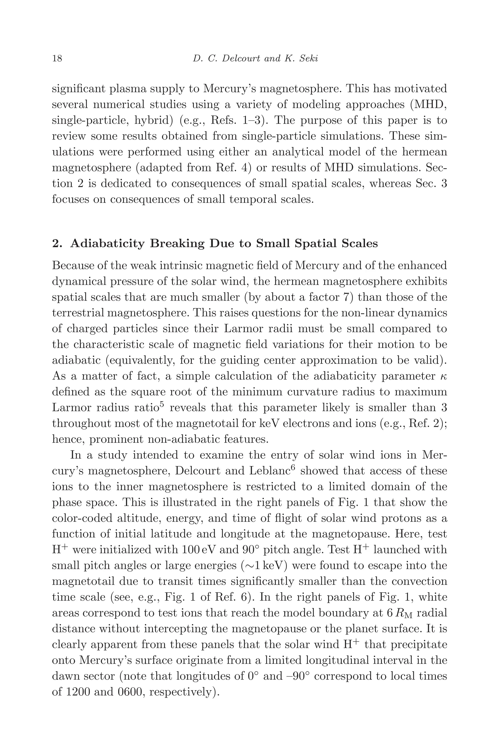
In a study intended to examine the entry of solar wind ions in Mer-
cury’s magnetosphere, Delcourt and Leblanc6
showed that access of these
ions to the inner magnetosphere is restricted to a limited domain of the
phase space. This is illustrated in the right panels of Fig. 1 that show the
color-coded altitude, energy, and time of flight of solar wind protons as a
function of initial latitude and longitude at the magnetopause. Here, test
H+
were initialized with 100 eV and 90◦
pitch angle. Test H+
launched with
small pitch angles or large energies (∼1 keV) were found to escape into the
magnetotail due to transit times significantly smaller than the convection
time scale (see, e.g., Fig. 1 of Ref. 6). In the right panels of Fig. 1, white
areas correspond to test ions that reach the model boundary at 6 RM radial
distance without intercepting the magnetopause or the planet surface. It is
clearly apparent from these panels that the solar wind H+
that precipitate
onto Mercury’s surface originate from a limited longitudinal interval in the
dawn sector (note that longitudes of 0◦
and –90◦
correspond to local times
of 1200 and 0600, respectively).
38.
March 16, 200613:47 WSPC/SPI-B368 Advances in Geosciences Vol. 3 ch03
On the Dynamics of Charged Particles in the Magnetosphere of Mercury 19
Fig. 1. (Right; from top to bottom) Final altitude, energy, minimum adiabaticity param-
eter κ, and time of flight of solar wind H+ as a function of initial longitude and latitude
at the magnetopause. Test H+ are traced until they reach the model boundary (i.e., the
magnetopause or a radial distance of 6 RM) or precipitate onto Mercury’s surface. (left)
Examples of (top) resonant and (bottom) non-resonant particles (adapted from Ref. 6).
In the right panels of Fig. 1, a prominent structuring of the precipi-
tating ion energy and time of flight can also be seen, that directly follows
from non-adiabatic transport in the mid-tail. Indeed, in their analysis of
non-linear particle dynamics in a field reversal, Chen and Palmadesso7
put
forward that, for some values (smaller than 1) of the κ parameter, particles
preferentially execute Speiser-type orbits whereas, for other κ values, most
of the particles experience prominent magnetic moment scattering and are
temporarily trapped inside the current sheet. This feature was interpreted
as the result of resonance between the fast meandering motion about the
mid-plane and the slow gyromotion about the normal field component. To
characterize these resonances, Chen and Palmadesso7
derived the follow-
ing empirical relationship: κn ≈ 0.8/(n + 0.6), where n is an integer ≥1.
These resonances coincide with the quasi-adiabatic regime put forward by
39.
March 16, 200613:47 WSPC/SPI-B368 Advances in Geosciences Vol. 3 ch03
20 D. C. Delcourt and K. Seki
Büchner and Zelenyi.5
They contribute to the formation of thin current
sheets and are responsible for the beamlets that are frequently observed in
the Earth’s plasma sheet boundary layer (e.g., Refs. 8 and 9).
In Fig. 1, resonant particles and associated beamlets are characterized
by short residence times (upper left panel), whereas quasi-trapped parti-
cles exhibit longer residence times as well as larger energies due to repeated
interactions with the current sheet and larger drift in the Y -direction (lower
left panel). It is thus clearly apparent from Fig. 1 that solar wind protons
entering Mercury’s magnetosphere exhibit an extreme sensitivity to initial
conditions at the magnetopause. That is, a slight change in injection posi-
tion leads to a large variation in the adiabaticity parameter κ, an effect
which is of importance for hybrid simulations and contrasts with the situ-
ation prevailing at Earth.
The small width of Mercury’s magnetotail has another important impli-
cation for the dynamics of charged particles. Indeed, in an attempt to esti-
mate the contribution of planetary ions to the magnetospheric populations,
Delcourt et al.2
showed that low-energy Na+
ions sputtered from the planet
surface may gain access to the magnetotail via convection over the polar
cap, in a like manner to low-energy ions upflowing from the topside iono-
sphere at Earth. In the magnetospheric lobes, these ions are subjected to a
prominent parallel energization due to an E × B related centrifugal effect
that is more pronounced (because of a larger angular speed of the convect-
ing field lines) than at the Earth. Once they interact with the magnetotail
current sheet, these Na+
ions are accelerated in a non-adiabatic manner and
may subsequently precipitate onto the planet surface, hence contributing to
regolith sputtering. Delcourt et al.2
showed that, on the whole, exospheric
Na+
form a substantial (several tenths of ions/cm3
) source of plasma for
the magnetotail. As envisioned in the “geopause” interpretation framework
of Moore and Delcourt,10
this raises the question of the net magnetospheric
contribution of planetary material versus that of the solar wind, especially
when the planet occupies a large volume of the magnetosphere as is the
case at Mercury.
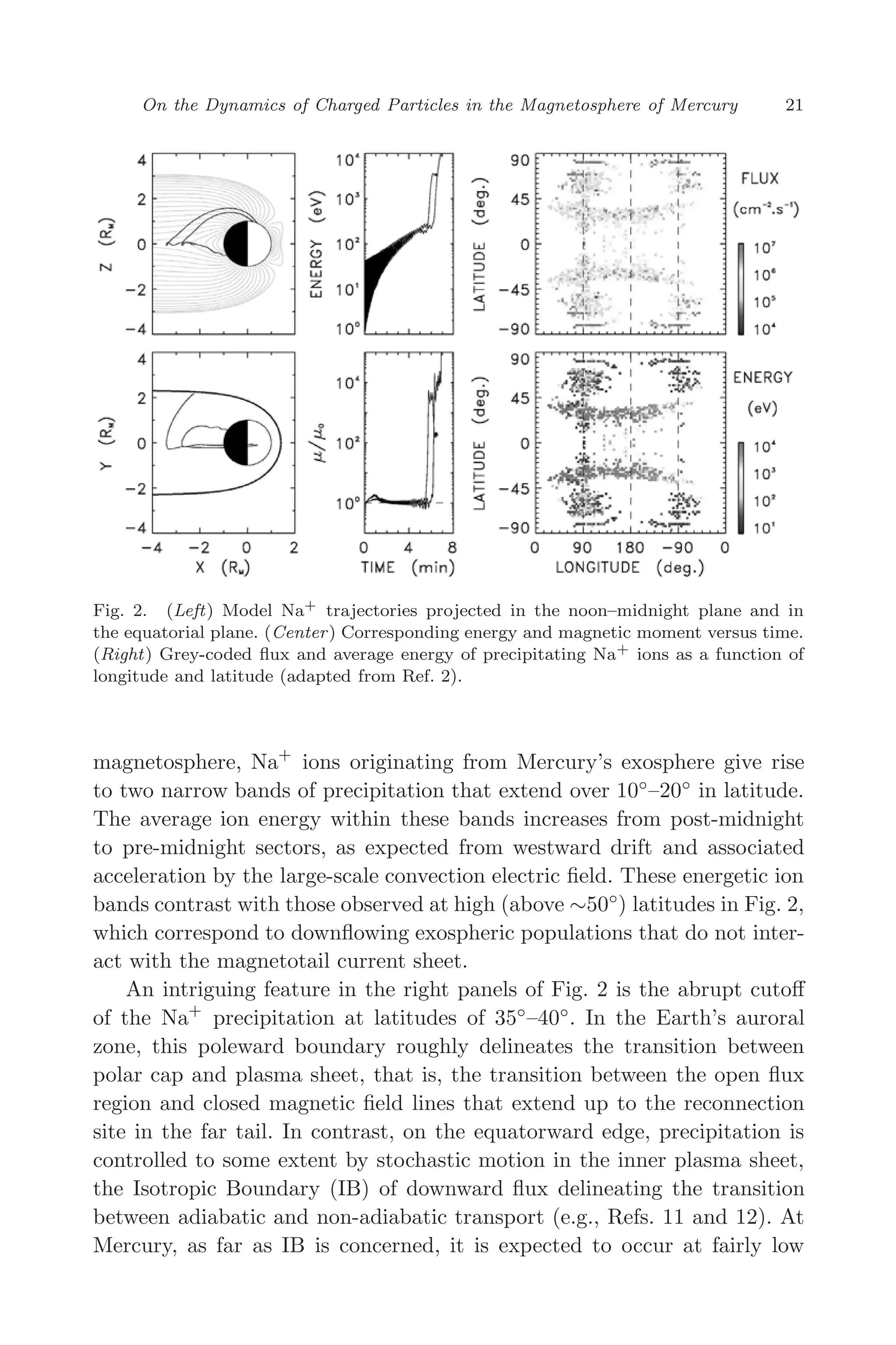
An example of planetary ion behaviors is shown in Fig. 2 that shows the
trajectories of test Na+
launched from two distinct latitudes in the dayside
sector (left panels), together with their energy and magnetic moment as a
function of time (center panels). As for the right panels of Fig. 2, they show
the results of systematic Na+
trajectory computations, with grey-coded flux
and energy of precipitating ions as a function of longitude and latitude. It
is apparent from the right panels of Fig. 2 that, after transport into the
40.
March 16, 200613:47 WSPC/SPI-B368 Advances in Geosciences Vol. 3 ch03
On the Dynamics of Charged Particles in the Magnetosphere of Mercury 21
Fig. 2. (Left) Model Na+
trajectories projected in the noon–midnight plane and in
the equatorial plane. (Center) Corresponding energy and magnetic moment versus time.
(Right) Grey-coded flux and average energy of precipitating Na+
ions as a function of
longitude and latitude (adapted from Ref. 2).
magnetosphere, Na+
ions originating from Mercury’s exosphere give rise
to two narrow bands of precipitation that extend over 10◦
–20◦
in latitude.
The average ion energy within these bands increases from post-midnight
to pre-midnight sectors, as expected from westward drift and associated
acceleration by the large-scale convection electric field. These energetic ion
bands contrast with those observed at high (above ∼50◦
) latitudes in Fig. 2,
which correspond to downflowing exospheric populations that do not inter-
act with the magnetotail current sheet.
An intriguing feature in the right panels of Fig. 2 is the abrupt cutoff
of the Na+
precipitation at latitudes of 35◦
–40◦
. In the Earth’s auroral
zone, this poleward boundary roughly delineates the transition between
polar cap and plasma sheet, that is, the transition between the open flux
region and closed magnetic field lines that extend up to the reconnection
site in the far tail. In contrast, on the equatorward edge, precipitation is
controlled to some extent by stochastic motion in the inner plasma sheet,
the Isotropic Boundary (IB) of downward flux delineating the transition
between adiabatic and non-adiabatic transport (e.g., Refs. 11 and 12). At
Mercury, as far as IB is concerned, it is expected to occur at fairly low
41.
March 16, 200613:47 WSPC/SPI-B368 Advances in Geosciences Vol. 3 ch03
22 D. C. Delcourt and K. Seki
latitudes since particles behave in a non-adiabatic manner throughout most
of the magnetotail. As for the poleward boundary, it can be seen in the
bottom left panel of Fig. 2 that it does not map into the far tail but at
distances of a few planetary radii and that it is due to the fact that ions
intercept the dusk magnetopause in the course of their interaction with the
current sheet. That is, in contrast to the situation prevailing at Earth, the
poleward boundary of precipitation in the right panels of Fig. 2 directly
follows from the finite ion Larmor radius. At large energies and/or large
mass-to-charge ratios, these Larmor radii become comparable to or larger
than the magnetotail width, in which case ions do not execute a full Speiser
orbit and are not reflected toward the planet. Here, it may actually be
suspected that this finite Larmor radius boundary at the poleward edge
of precipitation depends upon ion species (with a cutoff for heavy ions
occurring at lower latitudes than for H+
) and provides information of the
magnetotail structure, in a like manner to IB.
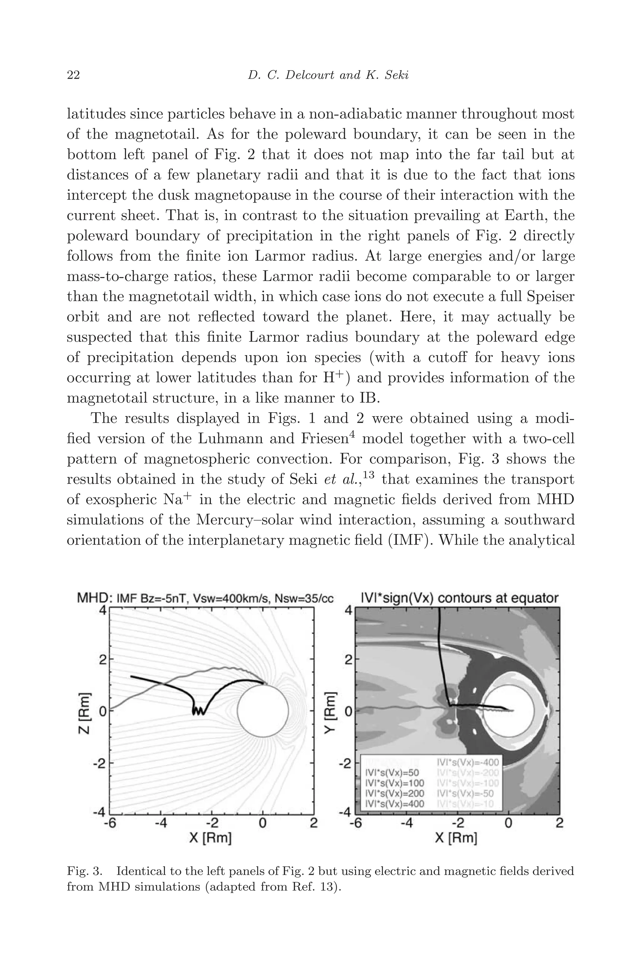
The results displayed in Figs. 1 and 2 were obtained using a modi-
fied version of the Luhmann and Friesen4
model together with a two-cell
pattern of magnetospheric convection. For comparison, Fig. 3 shows the
results obtained in the study of Seki et al.,13
that examines the transport
of exospheric Na+
in the electric and magnetic fields derived from MHD
simulations of the Mercury–solar wind interaction, assuming a southward
orientation of the interplanetary magnetic field (IMF). While the analytical
Fig. 3. Identical to the left panels of Fig. 2 but using electric and magnetic fields derived
from MHD simulations (adapted from Ref. 13).
42.
March 16, 200613:47 WSPC/SPI-B368 Advances in Geosciences Vol. 3 ch03
On the Dynamics of Charged Particles in the Magnetosphere of Mercury 23
model implicitly assumes the existence of a neutral line in the far tail, the
MHD results show the formation of a near-Mercury neutral line (NMNL)
near 2 RM radial distance (right panel of Fig. 3). In the terrestrial mag-
netosphere, the formation of such a neutral line near the planet is com-
monly associated with substorm activity. It is apparent from Fig. 3 that
the existence of such a NMNL can significantly alter the Na+
trajectories
and change the ratio of ions that precipitate onto the planet surface. That
is, ions that reach the region of tailward flow in the plasma sheet do not
return to the planet regardless of their κ parameter. These results suggest
that precipitation and recycling of planetary ions at Mercury depend upon
the magnetic activity and the large-scale convection pattern.
3. Adiabaticity Breaking Due to Small Temporal Scales
During the Mariner-10 pass of 1974, the magnetic field first pointed tailward
and abruptly turned northward after closest approach of the planet. Inter-
estingly, high-energy (several tens of keVs and above) electron injections
were recorded in conjunction with this rapid change of the magnetic field
orientation, a feature which is reminiscent of that observed during substorm
dipolarization at Earth. This suggests that the hermean magnetotail may
be subjected to substorm cycles as well (e.g., Ref. 14), although Luhmann
et al.15
put forward that these observations may provide indication of pro-
cesses directly driven by the solar wind.
If substorms occur at Mercury in a like manner to Earth, significant
particle energization is to be expected due to the electric field induced by
relaxation of the magnetic field lines. By means of two-dimensional simu-
lations, Ip16
actually demonstrated that protons may be accelerated up to
10–15keV during such reconfiguration events. On the other hand, because of
the short-time scales that characterize the hermean environment, it may be
anticipated that electrons are subjected to significant energization as well.
In a recent study, Delcourt et al.17
examined this issue using a rescaled ver-
sion of a time-dependent particle code previously developed to investigate
the dynamics of charged particles during substorms at Earth (see, Ref. 18
for details on the modeling technique).
An example of the results obtained by Delcourt et al.17
is presented
in Fig. 4. As mentioned above, characteristic time scales at Mercury are
expected to be smaller than those at Earth by about a factor 30 (e.g.,
Ref. 19), and a short-lived (5 s) dipolarization was accordingly considered
here. The left panels of Fig. 4 show selected electron trajectories during
43.
March 16, 200613:47 WSPC/SPI-B368 Advances in Geosciences Vol. 3 ch03
24 D. C. Delcourt and K. Seki
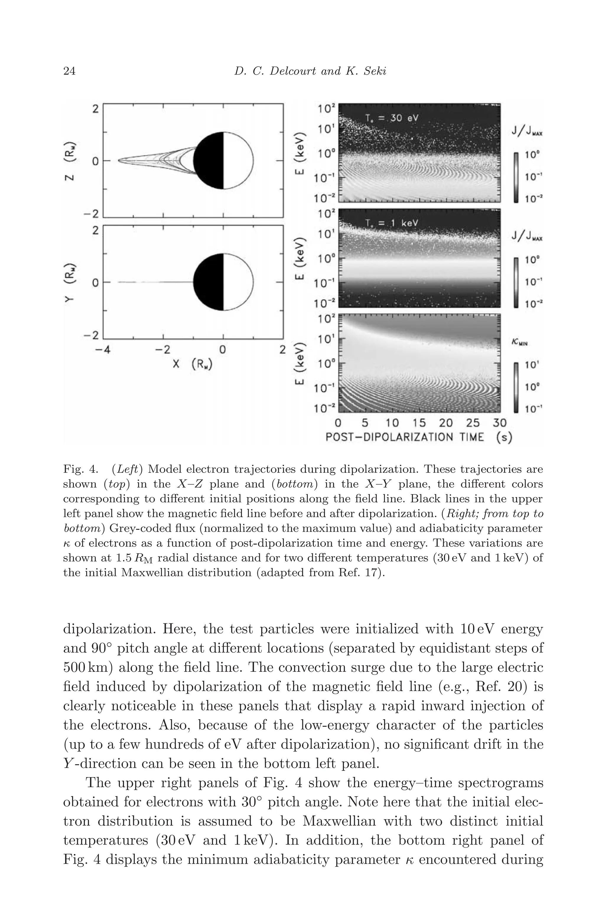
Fig. 4. (Left) Model electron trajectories during dipolarization. These trajectories are
shown (top) in the X–Z plane and (bottom) in the X–Y plane, the different colors
corresponding to different initial positions along the field line. Black lines in the upper
left panel show the magnetic field line before and after dipolarization. (Right; from top to
bottom) Grey-coded flux (normalized to the maximum value) and adiabaticity parameter
κ of electrons as a function of post-dipolarization time and energy. These variations are
shown at 1.5 RM radial distance and for two different temperatures (30 eV and 1 keV) of
the initial Maxwellian distribution (adapted from Ref. 17).
dipolarization. Here, the test particles were initialized with 10 eV energy
and 90◦
pitch angle at different locations (separated by equidistant steps of
500 km) along the field line. The convection surge due to the large electric
field induced by dipolarization of the magnetic field line (e.g., Ref. 20) is
clearly noticeable in these panels that display a rapid inward injection of
the electrons. Also, because of the low-energy character of the particles
(up to a few hundreds of eV after dipolarization), no significant drift in the
Y -direction can be seen in the bottom left panel.
The upper right panels of Fig. 4 show the energy–time spectrograms
obtained for electrons with 30◦
pitch angle. Note here that the initial elec-
tron distribution is assumed to be Maxwellian with two distinct initial
temperatures (30 eV and 1 keV). In addition, the bottom right panel of
Fig. 4 displays the minimum adiabaticity parameter κ encountered during
44.
March 16, 200613:47 WSPC/SPI-B368 Advances in Geosciences Vol. 3 ch03
On the Dynamics of Charged Particles in the Magnetosphere of Mercury 25
transport as a function of time and energy. A striking feature here is the
formation of bands of enhanced flux that gradually evolve with time. This
effect is obtained for low-initial temperature (top right panel) and vanishes
at higher initial temperatures (center right panel). The reason for this effect
may be understood by examining the κ variations in the bottom right panel
of Fig. 4. Indeed, it is apparent from this latter panel that electrons with
energies up to a few hundreds of eV have κ much large than unity. They
accordingly behave in an adiabatic (magnetic moment conserving) manner.
These test electrons however experience a different parallel energization
depending upon bounce phase at the dipolarization onset (violation of the
second adiabatic invariant), and Liouville theorem that states conservation
of the particle density in phase space leads to higher flux for those electrons
that experience larger energy gains.
On the other hand, it can be seen in the bottom right panel of Fig. 4
that, above a few hundreds of eV, electrons have κ of the order of unity
or below. These are accordingly subjected to magnetic moment scattering
which hampers the build-up of the above structuring due to differential
parallel energization. In other words, for T0 = 30 eV (top right panel), most
of the electrons are found to behave adiabatically with respect to the first
invariant but non-adiabatically with respect to the second one, whereas
for T0 = 1 keV (center right panel) the bulk of the electron population
behaves non-adiabatically with respect to the first invariant. Finally, note
that at high energies (several tens of keV), electrons are less sensitive to
the convection surge induced by the dipolarization and that they drift in
the immediate vicinity of the planet; hence their large κ parameter.
In the Earth’s magnetosphere, Mauk20
demonstrated that the bouncing
ion clusters frequently observed in the inner plasma sheet (e.g., Refs. 21 and
22) likely follows from such differential parallel energy gains and consequent
violation of the second adiabatic invariant during substorm dipolarization.
At Earth, reconfiguration of the magnetic field lines typically occurs on
time scales of the order of a few minutes and the above flux modulation
accordingly affect essentially ions that have comparable bounce periods.
In contrast, at Mercury, it is apparent from Fig. 4 that, because of small
temporal scales, such a flux modulation may be obtained for electrons and
it may be speculated that, in a like manner to bouncing ion clusters at
Earth, the build-up of bouncing electron clusters will provide information
on the dynamics of the magnetotail.
Finally, it was shown in Ref. 18 that, in the Earth’s magnetosphere, the
first adiabatic invariant may not be conserved during dipolarization which
allows for enhanced perpendicular energization. Given the relaxation time
45.
March 16, 200613:47 WSPC/SPI-B368 Advances in Geosciences Vol. 3 ch03
26 D. C. Delcourt and K. Seki
scale, such a non-adiabatic heating favors ions with large mass-to-charge
ratios because of their large gyration periods. This process may be respon-
sible for the species-dependent energization observed in the storm-time ring
current (e.g., Ref. 23). At Mercury, one may expect this non-adiabatic heat-
ing to affect plasma sheet H+
populations due to the short-time scale of
magnetic transitions.
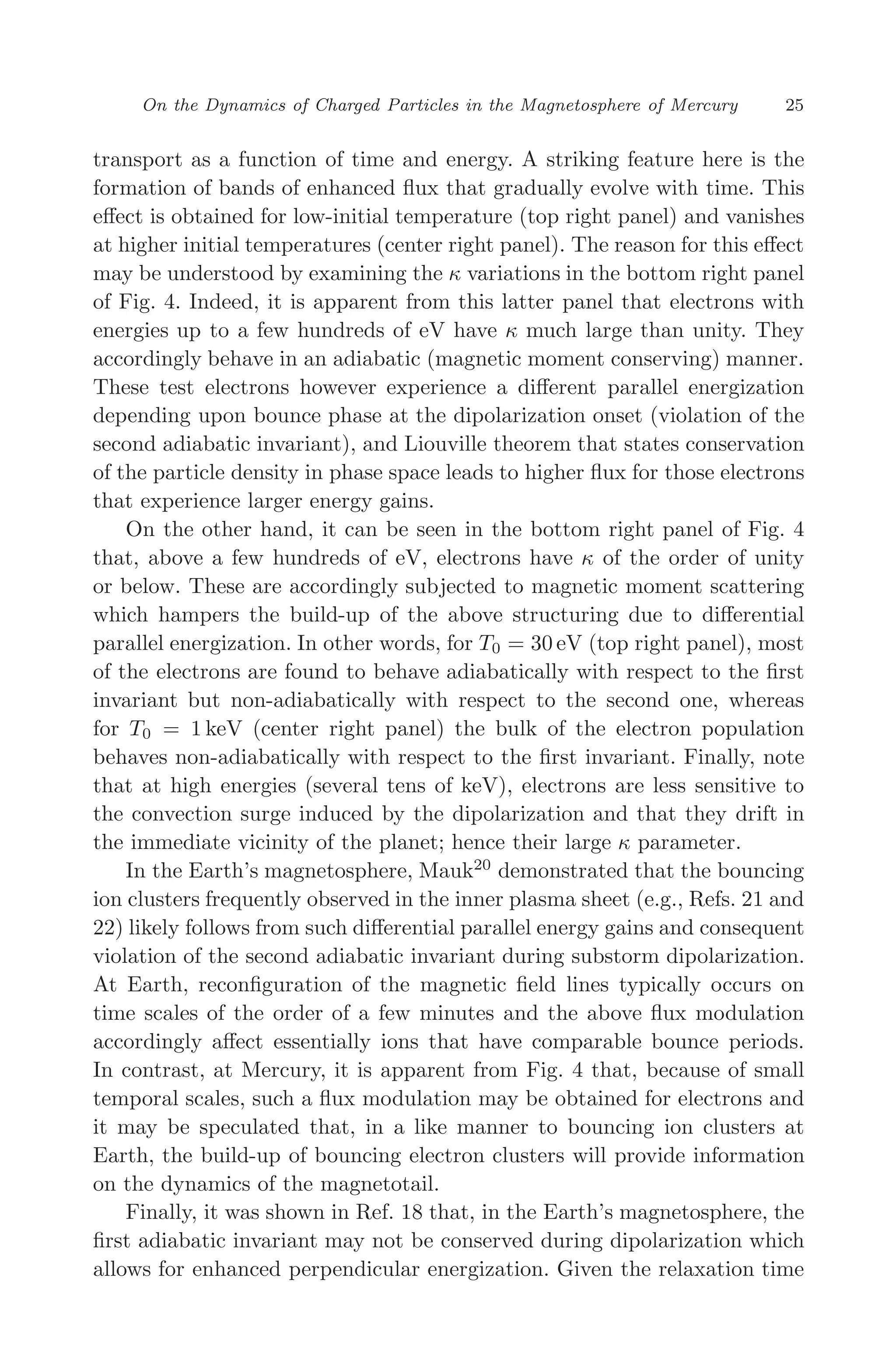
This is illustrated in Fig. 5 that shows model H+
trajectories in a
5-second dipolarization identical to that in Fig. 4. Here, test protons were
initialized with 100 eV energy and 90◦
pitch angle at different (grey-coded)
positions along the dipolarizing field line. It is clearly apparent from Fig. 5
that most of the test H+
are subjected to prominent magnetic moment
enhancement and energization (up to several tens of keV), with the excep-
tion of the ions initialized close to the planet surface that have small Larmor
radii and small gyration periods. One expects that a number of these
non-adiabatically accelerated ions will be lost at the dusk magnetopause
because of their large Larmor radii after dipolarization.
In this regard, note that ions at Mercury generally do not conserve
their magnetic moment even in the steady state case (see, e.g., Fig. 1) so
Fig. 5. Model H+ orbits during a 5-second dipolarization of the magnetic field lines:
(left) trajectory projections in noon–midnight and equatorial planes, (right) energy, and
magnetic moment versus time.
46.
March 16, 200613:47 WSPC/SPI-B368 Advances in Geosciences Vol. 3 ch03
On the Dynamics of Charged Particles in the Magnetosphere of Mercury 27
that a complex intrication of features due to both spatial and temporal
non-adiabaticity is to be expected (e.g., Ref. 24). A future study will be
dedicated to comparative analysis of proton and heavy ion transport under
such conditions.
4. Summary
Single-particle simulations of ion circulation within Mercury’s magneto-
sphere reveal prominent deviations from adiabaticity, be it due to small
spatial scales with respect to the particle Larmor radius or due to small
temporal scales with respect to the particle gyration period. Ions that cir-
culate in the inner magnetotail exhibit a prominent sensitivity to injection
conditions because of a sharp gradient in the magnetic field magnitude
and field line elongation. This leads to rapid changes from quasi-adiabatic
to quasi-trapped behaviors and vice versa. The small width of the her-
mean magnetotail also is of importance in this respect since ions with large
Larmor radii may not be reflected toward the planet after interaction with
the current sheet and intercept the dusk magnetopause. Ions are found
to be rapidly transported and energized within Mercury’s magnetosphere,
the significance of recycling and/or down-stream loss depending upon the
occurrence of reconnection in the magnetotail and upon the global convec-
tion pattern. The characteristic scales of Mercury’s magnetosphere are such
that electrons are found to behave non-adiabatically as well. In particular,
violation of the second adiabatic invariant due to the transient electric field
induced by dipolarization of the magnetic field lines may lead to short-
lived precipitation onto the planet surface as well as formation of bouncing
electron clusters in the inner magnetotail.
Acknowledgments
Part of this work was performed while D. C. Delcourt was residing at STEL,
Toyokawa, Nagoya University (Japan).
References
1. K. Kabin, T. I. Gombosi, D. L. DeZeeuw and K. G. Powell, Icarus 143 (2000)
397.
2. D. C. Delcourt, S. Grimald, F. Leblanc, J.-J. Berthelier, A. Millilo, A. Mura,
S. Orsini and T. E. Moore, Ann. Geophys. 21 (2003) 1723.
3. E. Kallio and P. Janhunen, Geophys. Res. Lett. 30 (2003) DOI 10.1029/
2003GL017842.
47.
March 16, 200613:47 WSPC/SPI-B368 Advances in Geosciences Vol. 3 ch03
28 D. C. Delcourt and K. Seki
4. J. G. Luhmann and L. M. Friesen, J. Geophys. Res. 84 (1979) 4405.
5. J. Büchner and L. M. Zelenyi, J. Geophys. Res. 94 (1989) 11,821.
6. D. C. Delcourt and F. Leblanc, Notes du Pôle de Planétologie (Institut Pierre
Simon Laplace, 2005), p. 12.
7. J. Chen and P. J. Palmadesso, J. Geophys. Res. 91 (1986) 1499.
8. M. Ashour-Abdalla, L. A. Frank, W. R. Paterson, V. Peroomian and L. M.
Zelenyi, J. Geophys. Res. 101 (1996) 2587.
9. J.-A. Sauvaud and R. A. Kovrazhkin, J. Geophys. Res. 109 (2004) DOI
10.1029/2003JA010333.
10. T. E. Moore and D. C. Delcourt, Rev. Geophys. 33 (1995) 175.
11. V. A. Sergeev M. Malkov and K. Mursula, J. Geophys. Res. 98 (1993) 7609.
12. P. T. Newell, Y. I. Feldstein, Y. I. Galperin and C.-I. Meng, J. Geophys. Res.
101 (1996) 10,737.
13. K. Seki, N. Terada, D. C. Delcourt and T. Ogino (abstract), SGEPSS, Kyoto,
Japan (2005).
14. G. L. Siscoe, N. F. Ness and C. M. Yeates, J. Geophys. Res. 80 (1975) 4359.
15. J. G. Luhmann, C. T. Russell and N. A. Tsyganenko, J. Geophys. Res. 103
(1998) 9113.
16. W.-H. Ip, Adv. Space Res. 19 (1997) 1615.
17. D. C. Delcourt, K. Seki, N. Terada and Y. Miyoshi, Annales Geophys. 24
(2006).
18. D. C. Delcourt, K. Seki, N. Terada and Y. Miyoshi, Ann. Geophys. 23 (2005)
3389.
19. G. L. Siscoe, N. F. Ness and C. M. Yeates, Substorms on Mercury?, J. Geo-
phys. Res. 80 (1975) 4359.
20. B. H. Mauk, J. Geophys. Res. 91 (1986) 15,423.
21. J. M. Quinn and C. E. McIlwain, J. Geophys. Res. 84 (1979) 7365.
22. M. Hirahara, T. Mukai, T. Nagai, N. Kaya, H. Hayakawa and H. Fukunishi,
J. Geophys. Res. 101 (1996) 7749.
23. D. G. Mitchell, P. C. Brandt, E. C. Roelof, D. C. Hamilton, K. C. Retterer
and S. Mende, Space Sci. Rev. 109 (2003) 63.
24. S. C. Chapman, Properties of single-particle dynamics in a parabolic mag-
netic reversal with general time dependence, J. Geophys. Res. 99 (1994)
5977.
48.
March 16, 200613:47 WSPC/SPI-B368 Advances in Geosciences Vol. 3 ch04
THE DAYSIDE MAGNETOSPHERE OF MERCURY
S. MASSETTI, S. ORSINI, E. DE ANGELIS, V. MANGANO,
A. MILILLO and A. MURA
Istituto di Fisica dello Spazio Interplanetario, IFSI-INAF, Roma, Italy
stefano.massetti@ifsi-roma.inaf.it
Many efforts are currently in progress to depict a realistic model of the Hermean
magnetosphere, also in the frame of the researches that will be performed by the
next space missions Messenger and BepiColombo. Although the magnetosphere
of this planet can be roughly approximated by scaling the Earth’s one (about
1:6.9), several differences are expected due to both the lack of an ionosphere,
which rise questions concerning the closure of the magnetospheric currents, and
the likely absence of a stable ring current. A remarkable feature, outlined by
the models, is represented by the wide area accessible by the solar wind plasma
on the Mercury’s dayside, due to the broad footprint of the magnetospheric
cusp regions. Moreover, the absence of a dense atmosphere/ionosphere implies
that a large faction of the impinging plasma can reach the planet’s surface. We
present the results obtained by comparing two modelization of the Mercury’s
magnetosphere by means of ad hoc modified Tsyganenko and Toffoletto–Hill
models. The analysis is focused on the dayside magnetospheric configurations
and plasma entry patterns, derived by taking into account the effect of the
magnetic reconnection with the interplanetary magnetic field. The role played
by the radial IMF component (Bx) is also discussed.
1. Introduction
We present preliminary results obtained by comparing two modelization
of the Mercury’s magnetosphere by means of ad hoc modified Tsyganenko
(T96) and Toffoletto–Hill (TH93) models, hereafter referred as T96* and
TH93*, respectively. The analysis is focused on the dayside magnetospheric
configurations and plasma entry patterns, derived by taking into account
the effect of the magnetic reconnection with the interplanetary magnetic
field (IMF). Figure 1 sketches the reconnection geometry on the dayside
magnetopause, and the related key parameters. We applied the stress bal-
ance condition to the de Hoffmann–Teller (HT) reference frame, moving
along the magnetopause at the rotational discontinuity produced by the
magnetic reconnection between the planet’s magnetic field and the inter-
planetary magnetic field (e.g., Refs. 1 and 2). Equations (1)–(5) permit us
29
49.
March 16, 200613:47 WSPC/SPI-B368 Advances in Geosciences Vol. 3 ch04
30 S. Massetti et al.
Fig. 1. Sketch of a reconnected field line on the dayside magnetopause, illustrating the
key parameters associated with the de Hoffmann–Teller (HT) reference frame: VA-SH and
VA-SP are the Alfvénic speed (tangent to the local magnetic field) on the magnetosheath
and the magnetospheric side, respectively; ϕ and θ are the angles formed by VA-SH
and VA-SP with the magnetopause (dashed grey line); VSH is the magnetosheath flow
velocity (black arrow tangent to magnetopause); and VHT is the HT reference frame
velocity (white arrow).
to determine the minimum (Vmin), peak (Vp), and maximum (Vmax) velocity
of the ions crossing the magnetopause along open field lines (please, refer
to Ref. 3 for a more detailed discussion):
VSH = −VA-SH cos ϕ, (1)
VHT = VSH + VA-SH cos ϕ, (2)
Vmin = VHT cos θ, (3)
Vp = VHT cos θ + VA-SP, (4)
Vmax = VHT cos θ + VA-SP + Vth. (5)
The acceleration of the injected plasma critically depends on the ratio
between the Alfvénic speed on the magnetospheric (VA-SP) and magne-
tosheath (VA-SH) sides. In this work, we assumed VA-SP = 5 VA-SH, while
the VA-SH speed was derived from the model. As in a previous analysis,3
the magnetosheath plasma velocity VSH, density NSH, and temperature TSH,
close to the magnetopause, were derived from the work of Spreiter et al.4
At
the orbit of Mercury, the presence of a significant Bx component causes the
plasma to precipitate mainly in the dayside hemisphere that is directly con-
nected to the IMF. This is due to the reduced plasma penetration through
the open magnetic field lines that are draped in the antisunward direction,
forming the polar cap regions. Our results suggest that the magnetic recon-
nection geometry causes the focusing of the plasma injection within confined
50.
March 16, 200613:47 WSPC/SPI-B368 Advances in Geosciences Vol. 3 ch04
The Dayside Magnetosphere of Mercury 31
areas of the magnetosphere. However, finite gyro-radius effects, grad-B and
E × B drifts are expected to spread out the plasma patterns as the injected
ions precipitate through the magnetosphere (e.g., Refs. 5 and 6).
2. Open Field Regions
In Fig. 2, we report the fraction of the Mercury’s surface that is crossed
by open magnetic field lines, mapping on the dayside magnetopause, as a
function of the solar wind pressure (Pdyn) and of the IMF Bz component.
On the left panels, the results we had obtained by means of the T96* model3
are shown: upper panel, IMF B = (0, 0, Bz) and Pdyn = 20 nPa; lower panel,
IMF B = (0, 0, −10) nT. On the right panels, we show the results derived
with the present model (TH93*) using the IMF geometries reported on
the legends: Bz-dominated (black lines) and three configurations with a
fixed Bx/By ratio along the nominal Parker’s spiral direction at Mercury
(gray lines).
In the T96* case, the open area is equally distributed in both northern
and southern hemispheres. In the TH93* case, the area is completely, or
Fig. 2. Fraction of Mercury’s surface that is characterized by open magnetic field lines,
mapping on the dayside magnetopause, as calculated by means of both the T96* (left
panels) and the TH93* (right panels) models. Upper panels: open field area as a function
of the IMF Bz component, for fixed solar wind pressure (Pdyn = 20 nPa): the black
lines mark the IMF B = (0, 0, Bz) configurations, while the gray lines show the results
obtained with the IMF aligned along the nominal Parker’s spiral direction (TH93* only,
since T96* is independent from Bx). Lower panel: open field area as a function of the
solar wind pressure, derived with the IMF configurations indicated in the legends.
51.
March 16, 200613:47 WSPC/SPI-B368 Advances in Geosciences Vol. 3 ch04
32 S. Massetti et al.
mainly, concentrated in the southern (northern) hemisphere for Bx posi-
tive (negative). The results obtained with the two models are similar in the
case of fixed solar wind pressure (Pdyn = 20 nPa, upper panels). For Bx/By
fixed along the Parker’s spiral direction (TH93* only), the open field area
increases progressively as a function of the total IMF strength. By allowing
the interconnection with the IMF Bx component, the TH93* model causes
a large fraction of the planetary surface to be exposed to the direct precipi-
tation of magnetosheath plasma, even when Bz ∼ 0, as previously discussed
by other authors (e.g., Ref. 7).
3. Plasma Penetration into Mercury’s Dayside
Magnetosphere
Figure 3 illustrates the results obtained by applying the stress balance
condition to the Mercury’s dayside magnetosphere, approximated by the
TH93* model. Calculations are made with a reference solar wind speed
with VSW = 430 km/s and density NSW = 76 cm−3
. In the test runs here
presented, three different interplanetary magnetic field configurations were
used, namely: IMF B = (30, 10, 0)nT (top), IMF B = (30, 10, 10)nT (mid-
dle), and IMF B = (30, 10, −10)nT (bottom), with a Bx/By ratio close to
the one expected at Mercury’s orbit (about 20◦
with respect to the radial
direction). The left panels show the foot-points of the magnetic field lines
on the surface of Mercury: closed (blue dots), open on the dayside (cusp
regions, red dots) and open tailward (polar caps, gray dots). Contrary to
the T96* model, the TH93* produces patterns in agreement with the Kallio
and Janhunen5
numerical simulations, thanks to the hemispherical asym-
metry introduced by the interconnection with the IMF Bx component. The
interconnection with the IMF radial component causes the magnetosphere
to be “open” also for zero, or positive, Bz component (Fig. 3, top and mid-
dle panels). When Bx is positive, the open hemisphere is the southern one,
where we can see the footprint of the local cusp. In this case, the northern
cusp becomes visible only when a significant IMF Bz component is applied,
but its extension is in any case smaller than the southern one. This is due to
the fact that most of the open field lines in the northern hemisphere cross
the magnetopause on the nightside side, where the magnetosheath flux is
strongly antisunward and few particles can to precipitate along the con-
vected field lines. When the sign of Bx is negative, the situation reverses,
and the northern hemisphere is the most exposed to the plasma injection.
The sign of the By component is responsible of the dawn–dusk asymmetry,
52.
March 16, 200613:47 WSPC/SPI-B368 Advances in Geosciences Vol. 3 ch04
The Dayside Magnetosphere of Mercury 33
Fig. 3. Preliminary results obtained by means of the TH93* model, with VSW =
430 km/s, NSW = 76 cm−3, under three different interplanetary magnetic field con-
figurations: IMF B = (30, 10, 0) nT (top), IMF B = (30, 10, 10) nT (middle) and IMF
B = (30, 10, −10) nT (bottom). Left panels: foot-point of closed (blue dots), open on the
dayside (cusps, red dots) and open tailward (polar cap, gray dots) magnetic field lines.
Right panels: estimation of the magnetosheath plasma entry through the magnetopause
(gray mesh), along the dayside open field lines (red lines). The flux is calculated by taking
into account the magnetic reconnection effects (Eqs. (1)–(5)), and by assuming that 50%
of the incoming ions are reflected back at the magnetopause boundary. The fluxes shown
have to be compared with the unperturbed solar wind flux of about 3.3×109 cm−2/s−1.
It can be noted that the highest fluxes are located near the subsolar region, where the
magnetosheath plasma is estimated to be about 3.5 higher than the upstream solar wind.
53.
March 16, 200613:47 WSPC/SPI-B368 Advances in Geosciences Vol. 3 ch04
34 S. Massetti et al.
with the cusp region shifted duskward (dawnward) in the northern (south-
ern) hemisphere for positive values. The same effect is observable on the
Earth, at high- and low-altitudes, from both particles and auroral data.
The right panels of Fig. 3 sketch the dayside magnetosphere of the planet,
with the magnetic field lines marked as above (red = open on the dayside,
gray = open on the tail). The color coded surface represents the estimated
magnetosheath particle flux injected along the dayside open field lines, and
mapped over the corresponding area of the magnetopause (gray mesh). The
fluxes are calculated by taking into account the energy gain produced by
the superimposition of the field line dragging caused by the magnetosheath
flow, and by the field line tension (as described by Eqs. (1)–(5)). Moreover,
it was assumed that 50% of the ions are reflected back by the magnetopause
boundary, that is, a transmission factor of 0.5, which is a typical value in
the case of the Earth (e.g., Ref. 8). To have an idea of the fraction of
ions that can actually reach the surface, the fluxes shown in Fig. 3 must
be multiplied by a factor of about 0.2, which is equivalent to a loss-cone
of 35◦
. In addition, finite gyro-radius effects, grad-B and E × B drifts are
expected to spread out, to some extent, the plasma precipitation patterns
depicted in Fig. 3, as the ions precipitate throughout the magnetosphere to
the planet surface (see e.g., Refs. 5 and 6). A big unknown in this context
is the poor knowledge of the intensity and geometry of the electric field,
which can strongly affect the displacement of the plasma away from the
injection regions. Figure 3 shows that the strongest fluxes are located near
the sub-solar region of the magnetopause, where the magnetosheath plasma
should be about 3.5 higher than the free solar wind (as expect on the base of
Spreiter et al.4
gasdynamic approximation). The energy distribution (not
shown) typically peaks on the equatorial side of the open field regions,
and then decreases gradually while moving toward the high latitudes,
as observed on the Earth’s LLBL, cusp and mantle magnetospheric
regions.3
4. Conclusions
We discussed some results from a modelization of the plasma entry on
the dayside magnetosphere of Mercury. This analysis was performed by
means of the TH93 model that we adapted ad hoc to reproduce the key
features of the planet. The results confirm our previous findings based on
a modified version of the Tsyganenko (T96) model,3
but display also other
54.
March 16, 200613:47 WSPC/SPI-B368 Advances in Geosciences Vol. 3 ch04
The Dayside Magnetosphere of Mercury 35
new aspects. In particular, the interconnection of the Mercury magneto-
sphere with the IMF Bx component produces a hemispheric asymmetry,
as discussed by other authors (e.g., Refs. 5 and 7). The magnetosheath
ions crossing the dayside magnetopause are subjected to acceleration at
the rotational discontinuity, generated by the merging of the IMF with the
planetary magnetic field. This mechanism can generate particles with ener-
gies up to several tens of keV, and fluxes of the order of 1010
cm−2
s−1
at
the magnetopause boundary, about 10% of which could reach the surface
of the planet (depending on the loss-cone).
The exact determination of these values is affected by several poorly
known parameters as the VA-SP/VA-SH ratio linked to the relative den-
sities on both sides of the rotational discontinuity at the magnetopause,
and the efficiency of the magnetic merging at the dayside of Mercury.
The latter plays a very important role: in fact, the rate of the magnetic
merging, which can be either “bursty” or “steady”, can heavily affect
the plasma distribution inside the magnetosheath. A high rate of dayside
magnetic merging would lead to a fast depletion of the plasma density
inside the magnetosheath, causing a sensible deviation from the Spre-
iter’s gasdynamic approximation. Under steady reconnection, the wide cusp
region of the Bx-interconnected hemisphere could be almost always “open”,
and the magnetosheath density would be locally close to the upstream
solar wind value. In this case, the fluxes calculated in this work would
rapidly decrease, approaching the values of the unperturbed solar wind at
Mercury’s orbit.
Acknowledgments
Authors wish to thank N. Tsyganenko, F. Toffoletto and T. Hill, together
with the NASA/Goddard Space Flight Center (NSSDC) for making
the magnetospheric T96, and TH93, models available to the scientific
community.
References
1. S. W. H. Cowley and C. J. Owen, Planet. Space Sci. 37 (1989) 1461–1475.
2. M. Lockwood and M. F. Smith, J. Geophys. Res. 99 (1994) 8531–8553.
3. Massetti et al., Icarus 166 (2003) 229–237.
4. J. R. Spreiter, A. L. Summers and A. Y. Alksne, Planet. Space Sci. 14 (1966)
223–253.
Auratum Imperial isthe Golden-banded-Lily of Japan which has
become so extensively known and popular since its introduction from
Japan by Mr. Gordon Dexter. It was first exhibited in July 1862, at
the Massachusetts Horticultural Exhibition. It first bloomed in
England same year. It was for sometime considered too tender for
the Canadas and New England states, but it proved to be hardy. We
have had ours twelve years, and give it only a slight protection. The
petals of the Auratum are snowy white with a golden band running
down the center of each, and freely spotted on the sides with deep
carmine red. They are very fragrant. Being of somewhat slender
growth, they need support. It does best in a warm sandy soil that
has been well manured and dug deeply. It is easily propagated from
the scales of the bulbs, each scale producing a small bulbet. They
should be planted in a box about a foot deep, in good friable soil
about three inches deep, and one inch apart. Sink the box in some
out of the way place in the garden, and water frequently. In a short
time small bulbs will be found forming on the base, which rapidly
grow, and must be transplanted out the second year in the bed; the
57.
third or fourthyear it will bloom. The little bulbets which form on the
mother bulb blossom a year earlier. They should be renewed in the
fall, after the foliage is dead. Plant in a bed about four inches deep,
and let them remain undisturbed for two years; then they are large
enough to bloom and should be transplanted into a permanent bed,
if required.
LONGIFLORUM LILIES.
These trumpet-shaped Lilies are charming in
appearance, quite hardy and fragrant. They
bloom in July or August, and continue in
beauty for a long time.
Longiflorum Japonicum blooms in July, and
is a fine dwarf bedder; color pure white,
with occasionally a greenish tinge outside.
Increases rapidly. Eximium bears a longer
flower, from six to nine inches in length, and
is more open at the mouth than the
common Longiflorum. Pure white and very
fragrant. Brownii is a native of Japan, and is a grand Lily of rare
beauty. It resembles Longiflorum in shape, but is larger and more
expanding; color white inside, exterior brownish-purple; stamens
rich chocolate, which forms a distinctive feature in this species. It
has been frequently confounded with Japonicum, but the difference
is very marked in the illustrations of the two, and are thus noted in
Messrs. Hallock & Thorp's "Catalogue of Lilies."
"Japonicum (Odorum, Japonicum Colchesterii). One of the most
beautiful and rarest Lilies in cultivation. It differs from Brownii and all
58.
the forms ofLongiflorum in many respects. Note the following
marked differences: Its broader, fewer and more spreading leaves,
the shape of the entire flower and broader claw of its divisions, its
shorter anthers with pollen tinged with red. The flower is solitary
and large, interior pure white, exterior of a pinkish-brown color,
tubular, bell-shaped, with spreading revolute tips; the bud shows a
rich golden tint. Bulb white, or whitish-yellow, never red or brown,
broad at the base, the scales which are somewhat narrow and acute
at the tip, the outer ones terminate at about two-thirds of the height
of the inner scales, whereas in Brownii the scales are broad, and all
pass up, overlapping, and terminate together at the apex of the
bulb, thus making the base much narrower than the apex."
It is a native of Japan, and is so exceedingly rare that it is priced at
$7.00, more than double the cost of any other in the list. Brownii
was priced, when a novelty at $4.00, but is now offered for $1.75.
Candidum, sometimes called Easter Lily, is one of the best known
and commonly grown of all the Lilies. It has been in cultivation for
59.
about three hundredyears. Bears a profusion of pure white fragrant
flowers in a compact head.
The double Tiger Lily is a very great improvement on the old single
variety. It is very double, and very showy. Wallacei is a new
Japanese variety, said to be magnificent; color, buff, spotted with
black.
Chalcedonicum or Scarlet Martagon is supposed to be the "Lily of the
field" mentioned in the Gospel. "It is magnificent, and its intense
scarlet is one of the finest shades in the whole vegetable kingdom. A
full bed is a most magnificent sight, and if suddenly looked at on a
bright day, has nearly the same effect for a moment as if looking at
the sun. It is much scarcer than it should be, and requires careful
culture, to be planted about six or eight inches deep, and watered in
the summer time. It pleases every one who is capable of being
pleased."
Lilies, as well as many other bloomers, are greatly improved by
thinning out the overplus, thus concentrating the sap to fewer
blossoms, which being thus liberally nourished, greatly increase in
size, and amply repay, by their superiority, for the loss in numbers.
Although this is a demonstrated fact, yet few have the courage to
prune where flowers are not very abundant, and many will not when
they are.
Those who have limited space are loth to devote much room to
Lilies, preferring plants that bloom continually throughout the
season, or that make more show. But it is not essential that the bed
should be devoted exclusively to lilies. For early spring blooming
there can be the Crocuses, Snowdrops, Hyacinths, Tulips, all of
which will bloom before the lilies, and after flowering can be taken
60.
up, i.e., theTulips and Hyacinths, and low bedding plants take their
places. Portulaca, Pansy, Ageratum, Mignonnette, Nemophila, Sweet
Alyssum, are all suitable for this purpose, and will not only make the
bed beautiful all the season with their blossoms, but will also be of
real benefit to the Lilies by shading their roots somewhat, and
keeping the soil more cool and moist.
Lilies must never be crowded; a foot or twenty inches is about right.
The soil should be dug deep and mixed with old rotted manure and
sand liberally, unless the soil is naturally sandy; if heavy, clayey soil,
it ought to have in addition to sharp sand, leaf mold and bog muck.
Plant the bulbs from six to eight inches deep, according to the size.
Last autumn, in planting my Lily, Tulip, Hyacinth, and other bulbs, I
made a little bed for each of pure sand, and then covered well with
soil, over which was put a blanket of old dressing, then, before
snow, a covering of boughs. The bulbs never came up so grandly,
nor grew so rapidly before. October is the best month for bedding
out, later will do, and many do not plant their Lilies till the frost is
out in the spring.
The two leading Lily growers of this country are John L. Child and V.
H. Hallock & Thorp, of Queens, N. Y.
61.
DOUBLE WHITE BOUVARDIA,"ALFRED NEUNER."
HIS is indeed a novelty among this class of valuable plants,
being the first double ever known. It is said to be equal if not
superior, in profuse blooming quality, and vigorous, healthy
growth, to the single white variety, Davidsonii, of which it is a
sport. The flowers are rather larger than those of the single
flowering, and composed of three perfect rows of petals, of the
purest waxy white color, each floweret resembling a miniature
Tuberose. The trusses are large and perfect, and are freely and
without interruption produced, even on the small side shoots, which
generally make no flowers on the single one. It is highly praised by
Mr. Thomas Meehan, florist and editor of the Gardeners' Monthly,
and by Mr. Henry A. Dreer, florist, of Philadelphia. "A grand thing,"
62.
says Mr. Meehan."Gives great satisfaction. It has excelled our
expectation," says Mr. Dreer.
My own specimen, about four inches in height, has twelve buds; two
small clusters are on side-shoots. The very fine illustration of this
Bouvardia we give our readers, has been kindly loaned by the Ellis
Brothers, Keene, N. H., who have a fine stock which they are
offering to the public.
Mr. Henry Cannell says, "Of all plants the Bouvardia, in our opinion,
excels for cut flowers, no matter either for button-hole bouquets or
table decoration; a spray of it is sure to be most prominent and
pleasing, and the odor of several kinds is deliciously refreshing, and
if well-grown they will more or less continue flowering nine months
out of the year. Strange to say, they need only the ordinary course of
cultivation of the winter-flowering Zonal Pelargonium; hitherto they
have been treated as a stove plant, whereas they only need a
temperature not higher than 50° to 60°, and in the summer to have
every attention, like a specimen Chrysanthemum, and on the first
appearance of frost to be taken into the house, and when growing
and flowering, to be supplied with liquid manure occasionally."
Our only experience with this genus has been with Bouvardia
Humboldtii Corymbiflora, and it has proved to be a very valuable
plant. Its pure white flowers are produced in large trusses; their
tubes are three inches in length, and very fragrant. It blooms very
freely and for a long period. This variety and Vreelandii are the best
single white.
Liantha is a dazzling scarlet, and a very profuse bloomer. Elegans,
salmon-scarlet; large and fine. Lady Hyslop, a light rose. Canspicua
is of a blood-red color, with whitish tube. Bicolor, a summer-
63.
flowering variety. Flowertube purple, with tint of blue and delicately
mottled flesh, tipped with white. These last we find, only in Cannell's
Floral Guide.
I have no difficulty in keeping my Bouvardia in the cellar, the leaves
drop off, but they come out anew in the spring.
CAMELLIA JAPONICA.
This is a very popular genus on account of their rich dark-green
leaves, and beautiful rose-like flowers. They are hardy greenhouse
plants, and thrive best in light loam mixed with sand and peat, but
will do well in light soil without the peat. It will not flourish in a
limestone soil. Mr. Vick gives the following in his Magazine:
"The Camellia Japonica was sent to England in 1739 by Father
Kamel, a missionary, for whom it was named. As a house-plant the
Camellia requires considerable care, on account of the tendency of
the flower buds to drop off. A northern exposure is best, and a
temperature of from forty to fifty degrees. When the buds are
swelling, water plentifully with warm water, but allow none to stand
in the saucer. Sponge the leaves once a week. In the spring put the
plant out in a shady place on the north side of a house or fence, not
under the drip of trees, and water it every day. Set the pots on a
hard bottom, so that no worms can get into them. They form their
flower beds during the summer, and at this time a good growth of
wood must be encouraged.
"In the Southern States the Camellia can be raised with not more
than ordinary care; at the North it must be considered entirely a
green-house plant, and as such will always be highly prized. We are
64.
often asked howit should be cared for as a house-plant, and to all
such, in the northern part of the country, where it is necessary to
maintain good fires in warm houses for several months of the year,
we have no hesitation in saying, let it alone, do not expend care and
labor where there is so little prospect of reward."
Camellias are of many hues, and some are beautifully striped. Gen.
Lafayette, bright rose, striped with white, imbricated. Bell Romann,
imbricated, large flower and petals, rose striated with bright
crimson. Matteo Molfino, petals cerise, with pure white band down
center. Mrs. Lurmann, crimson, spotted, very beautiful. Pure colors
of white, red, crimson, rose and carmine, can be obtained.
Azalea.—Shrubby green-house plants of easy cultivation. Very showy
and hardy. Like the Camellia, they are found in all the leading colors,
and also striped, blotched and spotted. They are both single and
double.
Alexander II, is white, striped with vermilion; edges of petals
fringed. Aurelia, white, striped with rosy orange, amaranth spots.
Flag of Truce, is a pure double white, very fine. Her Majesty, is rosy-
lilac, edged with white. Alice, rose, blotched with vermilion; double.
Mr. Vick gives the following directions: "Azaleas need a light soil of
sandy loam, to which should be added one-half leaf mold. Repotting
should be done in May, trimming the tops to bring them into shape.
Then plunge in some sheltered spot in the garden. In September the
plants should be brought in under cover, or into a cool room. They
do best when the temperature ranges from forty degrees at night to
sixty-five or seventy by day. The foliage should be showered once a
week, but care must be taken that the roots are not over-watered,
as they rot easily. Small plants bloom well, but their beauty increases
65.
as they getage and size. The flowers appear on the terminal shoots,
and are from one inch to two and a half inches in diameter.
"Azaleas if left to themselves will develop long shoots, that after a
time become naked below and are furnished with leaves only at their
extremities. Flower stems are formed on the new wood of each
summer's growth, consequently the amount of bloom, other things
being equal, depends upon the amount of new wood annually
produced. In order to have plants of good shape when they become
large, it is necessary to give attention to pinching and training them
from the first. The pyramid form, or more properly that of a cone,
and rounded at the top, is considered the best for the plant, as it
allows the greatest exposure of leaf-surface. Two principal methods
are adopted to regulate the growth and bring plants into shape: one
is by successive pinchings as the growth proceeds, the other by
allowing long shoots to grow and then bending and training them
down, thus causing many of the dormant buds along their whole
length to break and develop into shoots. A skillful combination of the
two methods is probably better than either exclusively."
Mr. John Dick, Philadelphia, has the largest stock of Camellias and
Azaleas, it is stated, in the United States. Their catalogue list of
these plants embraces more than a hundred varieties, to which we
refer our readers.
66.
E have cometo see your garden, said a gentleman with a
lady in company. They were from a neighboring town. This
two weeks after the heavy frost!
I told them my garden was in the stable, and thither I piloted them.
It was not a very small garden if it was in a stable. A hundred or
more plants had been hurriedly removed from the beds the day
before that freezing night! There they were, in the soiled pots just as
taken from the ground, or packed closely in boxes. Not very
attractive looking, in one sense, yet in another they were, for they
were bright, healthy appearing plants—leaves as fresh as when in
the open air, pretty Geraniums in bloom, a mass of Lobelia, attractive
with their tiny blue flowers, Coleus of varied hues, and even a few
Roses struggling into bloom.
Then we strolled among the despoiled beds, and the Pansies, so
large and pert, elicited admiration, and the Sweet Peas, just as
fragrant as though blight were not all around them, while dear little
Mignonnette seemed to have taken a new lease of life.
Yesterday I arranged in a shallow glass dish as handsome a bouquet
as I have had for the season. Sweet Clover sprays, Mignonnette and
fragrant Geranium leaves for the foundation all around the dish, a
few bunches of the little white wax balls, with their glossy leaves,
Geranium blossoms, and lots of Sweet Peas, from the most delicate
shades to the deepest, and bunches of splendid Pansies, Sweet
67.
Alyssum, a bitof purple Verbena here and there, and white-eyed
Phlox. It was just lovely.
When the evidence was sure that frost was surely coming, and a
great many plants must be taken up in a few hours' time, I was so
glad that full half of them were in pots. I could never have potted a
third of them in the time. The great object was to get them
sheltered, and the repotting could be done at my leisure.
But I almost changed my mind the other day after toiling several
hours at the business. So many pots to wash! then fill with fresh
earth, and set the plant. O dear, wasn't I tired! But then the wide
door was open, the day was lovely, and I rather think potting plants
in a stable is better than potting out of doors on a cold day, and
when one is in a great hurry. Plants that are in pots plunged in the
ground do not grow so many roots, and that is another advantage.
MY WINDOW BOX.
Perhaps I may as well tell you about my most important window
box. I had it made last autumn, and I was greatly pleased with it. It
is made of zinc, size one yard long, fourteen inches broad, seven
inches in depth. To give it strength it is framed at the top with wood.
You can have this of black walnut, or stained in imitation. You can
have the box painted any color you wish, or leave it unpainted. In
the center is Croton "Weismanni," on one side of it a fine
Eranthemum pictum; its green leaves look as though they were
painted with white streaks; on the other side, Acalypha
"Macafeeana." These are the largest plants in my box, and they do
not exceed ten inches in height. There are sixty plants in all, mostly
averaging six inches in height, but a few are quite small. They
68.
consist of verychoice Geraniums—some of them handsome-leaved—
variegated Abutilons, Lemon Verbena, two bright Achyranthes, six
very beautiful Coleuses, and four fine Begonias. There are others I
cannot stop to specify. You will see that I have filled my box with
what are, in themselves, beautiful without the aid of flowers, though
I expect to have a few of these by-and-by. I am perfectly satisfied
with it, however, just as it is. I had a large German Ivy growing out
of doors, which consisted of several long vines. This I planted in one
corner of the box, and then drooped and twined it on the outside.
The change to indoor life caused the large green leaves to fall off,
but already new ones have put forth, and the vines are rapidly
growing. Everything else had been previously prepared so that there
was no change in their leafage after being put in the box. It is a
great addition to the beauty of the box to have vines of pretty
foliage drape the sides. This autumn I have had it placed on a small,
low table with castors, so I can change the plants every week, and
thus avoid that turning toward the window which they always
assume if kept in one position.
I first put in drainage, and then filled the box with rich, mellow earth
in which was a mixture of one-third sand. I have been thus
particular in my description, for many, no doubt, who, like myself,
have to make the most of limited space, will be glad to know just
how to keep the greatest number of plants to the best advantage.
Not only is there a saving of room, but of labor, and it is more
cleanly.
HYACINTHS.
69.
Among the essentialsfor winter flowers are the bulbs. Of these the
hyacinth takes the lead. They are so easily grown; so lovely and so
fragrant that they are worthy of a place in every collection. They
should be planted so that the upper surface of the bulb is visible.
Water liberally and then put away in a cool dark place for several
weeks, six weeks is none too long, and some I allow to remain a
longer time, bringing them to the light at intervals so as to have a
succession of flowers. They are very effective planted in a group.
They are very pretty in hyacinth glasses, but this method ruins the
bulbs for future use. Planted out they will sometimes flower. The
best time to plant them in the border is in October, but the first of
November will do. It is a good plan to make a little bed of sand for
the bulb, and then cover with light porous soil. Hyacinths are classed
as tall and dwarf, single and double. The Roman Hyacinth is the
earliest bloomer, coming into flower about the holidays if started in
season. The spikes are small and flowers rather scattering. As soon
as the blooms fade, the stalk should be removed, and when the
leaves turn yellow, they can be cut off, and the bulb dried and
packed in paper bags and kept till time for autumn planting.
Hyacinth bulbs come from Holland. About Haarlem the rubbish
heaps are hyacinths, and the air is oppressive with their perfume.
In California there grows what is called the Twining Hyacinth. It
grows in the mountains, and twines about the bushes, sometimes
going up eight and ten feet. After it gets to the top of the bush and
rests awhile, it lets go of the earth and goes on blooming for
months, regardless of the burning sun. The flower stem breaks off
near the ground, and the flowers are kept swinging in the air
supported only by the bush about which it twines. The color is deep
70.
rose, and itis said to be very pretty. The picture of it certainly looks
attractive. It is a large cluster composed of dozens of blossoms.
For flowering in the house the Polyanthus Narcissus are very
desirable. They can be put into glasses as well as the Hyacinth, but
the most natural method is in a pot of earth, and the bulb is in a
better condition for after use. The Jonquils are also pretty.
Snowdrops, Scillas and the Crocus are cheap bulbs, and planted in
the autumn will show their bright, sweet faces soon after the snow is
gone. They are also very fine for house culture. Should be planted in
groups.
Tulips ought to have a place in every garden. They make a brilliant
show in the Spring, when the beds are bare of other flowers, and
afford bloom for a long time, if a good assortment is selected. The
pretty little dwarf Duc Van Thols are early bloomers and very gay.
They are admirable also for the house, and by planting in
September, will come into flower in December. There are early single
and double Tulips, and also late bloomers, so that by having a
variety, the border may look gay for a long time. The Parrot Tulips
are large and very brilliant in color, and picturesque in appearance.
All of these varieties succeed in ordinary garden soil. They ought to
be planted in October or November, about four to six inches apart,
and about four inches under the surface. Before severe frost they
need to be protected by branches of evergreen, straw or leaves.
After blooming, and the leaves have died down, they can be taken
up, dried and stored till autumn, if the bed is needed for other
flowers.
The Bulb catalogues issued by leading florists in the autumn, and
sent free to all applicants, will enable you to select just what you
71.
want.
INSECTS.
In a workof this character it seems needful to treat more fully of
those pests which prove so destructive to plant life, than we have in
our brief references.
The Aphis or green louse is the one that most frequently infests our
plants, and the rapidity with which it multiplies, is astonishing.
Reaumer has proved that in five generations one aphis may be the
progenitor of six thousand millions, and there may be ten
generations in a year!
The method most generally adopted for their destruction is
fumigation with tobacco. As this is attended with considerable
difficulty, a weak solution may be used quite as effectively. We have
had no experience with either method, having used another with
good success for several years. This is white hellebore which we
usually apply in the powder when the Rose-bushes are wet with dew
or rain, bending the branches over, so that the application can be
made chiefly on the under side of the leaves, where the pests are
found. Two or three times proves sufficient. For our house plants we
usually make a solution, by putting half an ounce of the hellebore
into pretty warm water, and letting it stand for several hours, stirring
it up however, before spraying the leaves. Afterward, the plants need
to be washed.
72.
For the Scalea strong solution of soap-suds applied with a sponge or
a small stiff brush. A tooth brush is very suitable for this purpose.
For Mealy Bug, a mixture of one part alcohol and three parts water,
applying with a feather, or what is better, a camel hair brush.
Another method is to use kerosene in the same way. A florist who
has practiced this for eight years, says it is sure death to the insect.
The feather should be brushed all over the mealy-looking substances
found usually in the axils of the leaves.
Worms in Pots. Lime water is a safe and effectual remedy for the little
white worms often found in the soil. Slake the lime in water and
after it has settled, pour off the clear water and drench the earth.
Ants. Various remedies have proved effective. One is to take a vial or
a cup nearly filled with sweet oil, and sink it in the ground where the
ants resort, so that the rim is on a level with the surface. The ants
are very fond of it, but it is sure death to them.
A German writer says that carbolic acid and water will drive ants
away from any grounds—one hundred parts of water to one of the
acid. Mix in a tub and stir repeatedly for twenty-four hours, taking
off the scum that rises to the top.
Kerosene or coal-oil mixed with water has proved very successful in
the destruction of noxious insects and grubs. A tablespoonful of the
oil to two gallons of water is the rule for tender plants; for hardy
ones it will be necessary probably to have it of greater strength. As
the compound does not mix readily, it needs to be thoroughly
stirred, and then quickly applied. The best way is to draw it back and
forth a few times in a syringe, and then apply.
73.
Water tainted withcoal-oil, poured into little holes made in mole
tracks, will, it is said, drive them effectually away.
74.
INDEX OF FLORISTS.
Forthe convenience of our readers who may wish to procure
varieties of plants of which we have treated in this work, we give the
address of reliable florists who make a specialty of those connected
with their address. All of them will furnish their catalogues free when
requested.
Pansies. Seeds for the Wild Garden. B. K. Bliss & Sons, New
York City.
Verbenas, Petunias, Fuchsias. C. E. Allen, Brattleboro, Vt.
Geraniums. Innisfallen Greenhouses, Springfield, Ohio.
Pelargoniums, Ornamental Foliage Plants, Gloxinias. John
Saul, Washington, D. C.
Gladiolus, Single Dahlias, Novelty Dahlia. V. H. Hallock &
Thorp, Queens, N. Y.
Coleuses—New Hybrids, Dracænas. H. A. Dreer, Philadelphia,
Pa.
Chinese Primroses, New Primula, Double White Bouvardia. Ellis
Brothers, Keene, N. H.
New Monthly Pelargoniums. John G. Heinl, Terre Haute, Ind.
Wistaria. E. H. Ellwanger, Rochester, N. Y.
75.
Amaryllis, Rare Varieties.John L. Child, Queens, N. Y.
Lilies a Specialty. John L. Child; V. H. Hallock & Thorp,
Queens, N. Y.
Camellias and Azaleas. John Dick jr., 53d st., and Darby
Road, Philadelphia, Pa.
76.
AUTHOR'S NOTES.
Vick's IllustratedMagazine is the best Floricultural Monthly we know
of for amateurs. We are indebted to it for much of the information
we have obtained respecting the culture of flowers, and have drawn
largely from its pages in this work. There is a finely colored
frontispiece in each number, and it is otherwise fully illustrated. Its
entire arrangement evidences the fine æsthetic taste of its editor
and publisher. It is very low at $1.25 per year. Beautifully bound
vols., $1.75. Mr. James Vick, Rochester, N. Y.
The Gardener's Monthly and Horticulturist takes a wider range,
treating not only of Flowers, but also of Fruit and Vegetable
Gardening, Natural History and Science, Forestry, etc. The ample
Notes pertaining to the several departments, by its editor, Mr.
Thomas Meehan, are of special value. Published by Chas. H. Marot,
Philadelphia, Pa., at $2.10 per annum.
77.
"AN ESSAY ONROSES."
NOTICES OF THE PRESS.
Mrs. M. D. Wellcome of Yarmouth, Me., whose pleasant and helpful
"Talks About Flowers" are familiar to the readers of The Journal, has
published in a neat pamphlet, An Essay on Roses, which was read
before the Maine Pomological Convention last March, and has since
been revised and enlarged for publication. This essay treats the
subject historically and descriptively. It considers the classification of
Roses, tells what Roses to plant, gives suggestions as to the best
mode of culture, and furnishes a list of the best hybrids and of the
best ever-blooming varieties. Mrs. Wellcome writes with enthusiasm,
and from a thorough knowledge and a considerable experience. All
lovers of roses, and all amateur horticulturists will find the little
monograph interesting and suggestive.
Boston Journal.
The valuable and instructive Essay on Roses read before the Maine
Pomological Convention by Mrs. M. D. Wellcome, has been issued in
a neat pamphlet.... Our readers who are familiar with Mrs.
Wellcome's writings, will know how to value this production of her
busy pen.
Portland Transcript.
Our well-appreciated correspondent, Mrs. M. D. Wellcome, has
published in a neat pamphlet, an essay upon "Roses."... It is an
78.
interesting and practicallittle manual, and will prove a valuable aid
to young horticulturists.
Zion's Herald.
The Waterville Mail says: "Of this essay it is sufficient to say that it
was prepared by a graceful writer,—a well-known contributor to the
literary department of several prominent Journals, and a skillful
florist—and that it secured the approbation of the Convention before
whom it was read, and the representatives of the agricultural press."
Rev. J. M. Orrock, editor of Messiah's Herald, after describing the
work, adds: "The author says in her introduction, 'I have brought
you a bouquet of Roses, and there is little of my own but the string
that binds them.' It is indeed, a pretty bouquet, and we hope many
of her friends will want to see and enjoy it."
Mr. Samuel L. Boardman Esq., editor of the Home Farm, says: "This
little booklet about Roses is just the plain, sensible guide all amateur
growers will be profited by reading. There is just enough of history
and sentiment in its opening pages, ample directions for culture,
treatment, etc., closing with descriptions of the most desirable
Roses, and lists from which to make selections for larger cultivators.
Mechanically, the little book is as delicate as a rosebud; and every
lover of this queenly flower should procure a copy."
The "Essay" is issued in a neatly illustrated pamphlet of 24 pages,
with ornamental cover. Price 15 cents. For sale by the author,
Yarmouth, Me.
79.
GERANIUMS!
We offer afine assortment of Geraniums at 10 CENTS EACH, for
your selection; or we will send 16 FINE SORTS of our own
selection, all labeled, prepaid, by mail, for a remittance of $1.25. We
have by far the largest stock of Geraniums in this country.
Roses, Ever Blooming.
We have a fine collection of Roses that we offer, strong flowering
plants, labeled, at 10 CENTS EACH, your choice; or we will send
16 FINE PLANTS of our own selection, prepaid, by mail, for a
remittance of $1.25.
We also offer a fine assortment of all kinds of flowering plants at the
above low price. Send for a catalogue.
Address,
INNISFALLEN GREENHOUSES,
SPRINGFIELD, O.
NEW HYBRID TEAS.
80.
This new classof ROSES combine HARDINESS, CONSTANT
BLOOM, and DELICATE COLORING. They originated in England,
and are now offered for the first time in this country. For full
description of these Roses, and price, send for catalogue.
E. C. ALLEN, Brattleboro, Vermont.
FREE!
We wish to obtain 25,000 New Subscribers to
THE FLORAL MONTHLY
during the next few months, and we propose to give to every reader
of this paper
Fifty Cents Worth of Choice Flower Seeds.
Our offer is to send, Free of Cost, 50 cents worth of Choice Flower
Seeds to each and every one who will send us 25 two cent postage
stamps for the FLORAL MONTHLY one year. Seeds sent free by
return mail. Specimen copies free. Address
W. E. MORTON & CO., FLORISTS, 615 Congress Street,
Portland, Me.
(NATURAL FLOWERS PRESERVED TO LAST FOR YEARS.)
81.
Transcriber's Note:
Punctuation hasbeen standardised, and typographical errors such as missing or reversed
letters have been silently corrected.
Variations in hyphenation (such as greenhouse and green-house), and obsolete or variant
spelling have been preserved. In particular, variations in the spelling of some botanical
names have been left as printed in the original book.
In the Table of Contents, the entry "A Talk About Pansies" was printed as "Pansies"; this
has been changed to match the chapter title as printed on page 33.
The following changes were also made:
Pg 82, Verschaffellii changed to Verschaffeltii: (Verschaffeltii, we fear).
Pg 109, Ainwick changed to Alnwick: (a visit to Alnwick Castle).
82.
*** END OFTHE PROJECT GUTENBERG EBOOK TALKS ABOUT
FLOWERS. ***
Updated editions will replace the previous one—the old editions
will be renamed.
Creating the works from print editions not protected by U.S.
copyright law means that no one owns a United States
copyright in these works, so the Foundation (and you!) can copy
and distribute it in the United States without permission and
without paying copyright royalties. Special rules, set forth in the
General Terms of Use part of this license, apply to copying and
distributing Project Gutenberg™ electronic works to protect the
PROJECT GUTENBERG™ concept and trademark. Project
Gutenberg is a registered trademark, and may not be used if
you charge for an eBook, except by following the terms of the
trademark license, including paying royalties for use of the
Project Gutenberg trademark. If you do not charge anything for
copies of this eBook, complying with the trademark license is
very easy. You may use this eBook for nearly any purpose such
as creation of derivative works, reports, performances and
research. Project Gutenberg eBooks may be modified and
printed and given away—you may do practically ANYTHING in
the United States with eBooks not protected by U.S. copyright
law. Redistribution is subject to the trademark license, especially
commercial redistribution.
START: FULL LICENSE
PLEASE READ THISBEFORE YOU DISTRIBUTE OR USE THIS WORK
To protect the Project Gutenberg™ mission of promoting the
free distribution of electronic works, by using or distributing this
work (or any other work associated in any way with the phrase
“Project Gutenberg”), you agree to comply with all the terms of
the Full Project Gutenberg™ License available with this file or
online at www.gutenberg.org/license.
Section 1. General Terms of Use and
Redistributing Project Gutenberg™
electronic works
1.A. By reading or using any part of this Project Gutenberg™
electronic work, you indicate that you have read, understand,
agree to and accept all the terms of this license and intellectual
property (trademark/copyright) agreement. If you do not agree
to abide by all the terms of this agreement, you must cease
using and return or destroy all copies of Project Gutenberg™
electronic works in your possession. If you paid a fee for
obtaining a copy of or access to a Project Gutenberg™
electronic work and you do not agree to be bound by the terms
of this agreement, you may obtain a refund from the person or
entity to whom you paid the fee as set forth in paragraph 1.E.8.
1.B. “Project Gutenberg” is a registered trademark. It may only
be used on or associated in any way with an electronic work by
people who agree to be bound by the terms of this agreement.
There are a few things that you can do with most Project
Gutenberg™ electronic works even without complying with the
full terms of this agreement. See paragraph 1.C below. There
are a lot of things you can do with Project Gutenberg™
electronic works if you follow the terms of this agreement and
help preserve free future access to Project Gutenberg™
electronic works. See paragraph 1.E below.
85.
1.C. The ProjectGutenberg Literary Archive Foundation (“the
Foundation” or PGLAF), owns a compilation copyright in the
collection of Project Gutenberg™ electronic works. Nearly all the
individual works in the collection are in the public domain in the
United States. If an individual work is unprotected by copyright
law in the United States and you are located in the United
States, we do not claim a right to prevent you from copying,
distributing, performing, displaying or creating derivative works
based on the work as long as all references to Project
Gutenberg are removed. Of course, we hope that you will
support the Project Gutenberg™ mission of promoting free
access to electronic works by freely sharing Project Gutenberg™
works in compliance with the terms of this agreement for
keeping the Project Gutenberg™ name associated with the
work. You can easily comply with the terms of this agreement
by keeping this work in the same format with its attached full
Project Gutenberg™ License when you share it without charge
with others.
1.D. The copyright laws of the place where you are located also
govern what you can do with this work. Copyright laws in most
countries are in a constant state of change. If you are outside
the United States, check the laws of your country in addition to
the terms of this agreement before downloading, copying,
displaying, performing, distributing or creating derivative works
based on this work or any other Project Gutenberg™ work. The
Foundation makes no representations concerning the copyright
status of any work in any country other than the United States.
1.E. Unless you have removed all references to Project
Gutenberg:
1.E.1. The following sentence, with active links to, or other
immediate access to, the full Project Gutenberg™ License must
appear prominently whenever any copy of a Project
Gutenberg™ work (any work on which the phrase “Project
86.
Welcome to ourwebsite – the perfect destination for book lovers and
knowledge seekers. We believe that every book holds a new world,
offering opportunities for learning, discovery, and personal growth.
That’s why we are dedicated to bringing you a diverse collection of
books, ranging from classic literature and specialized publications to
self-development guides and children's books.
More than just a book-buying platform, we strive to be a bridge
connecting you with timeless cultural and intellectual values. With an
elegant, user-friendly interface and a smart search system, you can
quickly find the books that best suit your interests. Additionally,
our special promotions and home delivery services help you save time
and fully enjoy the joy of reading.
Join us on a journey of knowledge exploration, passion nurturing, and
personal growth every day!
ebookbell.com