Download as PDF, PPTX


![18
Sequential
Kaiser et al. (2010) Frontiers in Neuroinformatics
Hilgetag & Kaiser PLoS Comput. Biol. (in preparation)
Hierarchy
getag and others Hierarchical organization of macaque and cat cortex
V3
V2
PIP
VOT
AITv STPa
TH
AITd
V4
CITv
V11
2
4
3
5
8
7
6
11
10
9
46
CITd FEF
FSTPITd
V3A
VP
V4t
LIP
PO
MSTl
DP
7aPITv
VIPMSTd
TF
STPp
MT
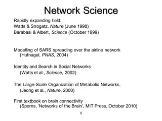
mal hierarchical enumeration of primate visual areas, in which each area is placed at the lowest level possible
straint suggested by Van Essen & Felleman (1996) and Crick & Koch (1998)). In this optimal 11-level scheme,
aced on the lowest level of the area's distribution in all optimal 11-level hierarchies, see ¢gure 16. To verify that
me with lower positions for the areas existed, we attempted to compute optimal hierarchies with ten levels, but
xtensive computations. Most connections between the areas are omitted for simplicity's sake; however,
h lateral contributions in their connectivity patterns are shown. This points out a network that may implement a
ystem within the primate visual system, see ½ 4(e). The constraint violations for this optimal arrangement are
T4MSTd, FST5TF, and their respective counterparts. Dashed lines denote these violations in the scheme.
with identical hatching have ¢xed relative, or absolute, positions in all optimal 11-level hierarchies computed, see
cheme is arranged so as to represent the functional subdivisions of the primate visual system, with the left side
ventral and the right side the dorsal stream.
area
5
10
level
V1
V2
VP
V3
PIP
V3A
V4
PO
MT
V4t
VOT
DP
VIP
MSTd
LIP
MSTl
PITv
PITd
FST
7a
STPp
CITv
CITd
FEF
STPa
AITv
46
TF
TH
AITd
ribution of primate visual areas in 108 optimal hierarchies with 11 levels. Constraint violations are: FST4MSTd
ncy in all solutions: 12%), FST5TF (9%), FST STPp (8%), LIP ˆ PITv (7%), LIP4MSTd (5%),
Particularly striking were the very stable clusters of
somatosensory-motor areas.
The binary classi¢cation of these connectivity data,
and their subsequent OSA, led to very similar cluster
structures as the categorization of existing connections in
three classes. The main subdivisions detailed above for
the balanced OSA condition were also recognizable for
balanced OSA arrangements of the binary data, even
though the ¢rst two groups of somatosensory-motor and
`limbic'areas were more strongly subdivided in the binary
data. The correlation between the cluster-count summa-
ries for the quaternary and binary data (655 optimal
arrangements) under balanced OSA was R ˆ 0.61. The
cluster arrangements of the binary data were reduced to
building-block structures at a repulsion weight of ten, and
248 optimal arrangements obtained under this condition.
All areas came together in one cluster for an attraction
weight of 21.
There are two principal ways of interpreting the
graded strengths of existing connections for this set of cat
connectivity data. In the `optimistic' interpretation, which
we followed in the above analysis of the quaternary data,
the numerical values assigned to the di¡erent strengths
directly re£ect the absolute anatomical strengths or densi-
ties of the connections. On this assumption, it is possible
to evaluate the di¡erent connections as if, for instance,
any intermediate-strength connection (with a value of
two) is indeed about twice as strong as two weak connec-
tions (with a strength value of one). In this view, the
connection strength classes approximate interval data. In
a more conservative interpretation, on the other hand,
the strength values are solely numerical labels for ranks of
di¡erent connection densities, which are considered
ordinal or nominal. In this case, a direct numerical
comparison of di¡erent connection categories would not
be possible. We considered this possibility by modifying
our OSA algorithm in such a way that di¡erent connec-
tion categories would be considered independently from
each other during the optimizations. This was achieved
by giving all connections of a particular category such
high weights that the arrangement of areas possessing this
connection could not be a¡ected, even if all connections
of lower ranks together exerted a contrary in£uence. In
this way, the overall arrangement was ¢rst shaped by the
optimization of the highest ranks, then by next highest and
so on, while the di¡erent ranks did not directly interfere
with each other. The weights of the absent and unknown
connections were determined as means of the weights for
the existing connections, weighted by the frequency of
connections in a particular strength category. Applying
such a modi¢ed OSA to the ¢nely graded cat connectivity
data yielded a unique cluster arrangement, which
resembled the main subdivisions obtained for the balanced
OSA of the quaternary data. Di¡erences between the
Connectivity clusters in macaque and cat cortex C.-C. Hilgetag and others 103
Phil.Trans. R. Soc. Lond. B (2000)
areas
V1
V2
V3
MT
V3A
V4t
VP
PIP
V4
VIP
MSTl
PO
LIP
MSTd
FST
DP
FEF
7a
STPp
46
CITd
TH
AITd
CITv
PITv
AITv
TF
PITd
MIP
MDP
STPa
VOT
V1
V2
V3
MT
V3A
V4t
VP
PIP
V4
VIP
MSTl
PO
LIP
MSTd
FST
DP
FEF
7a
STPp
46
CITd
TH
AITd
CITv
PITv
AITv
TF
PITd
MIP
MDP
STPa
VOT
Figure 8. Cluster-count summary of all clusters identi¢ed by ¢xed-radii NPCA in 2D-NMDS representations of primate visual
connectivity.
Topological
SpatialTemporal
Period concatenation in neocortical rhythms
Author's personal copy
0.1 1
102
103
<v(τ)>
REM
0.1 1
102
103
Wake
0.1 1
102
103
N1
0.1 1
102
103
<v(τ)>
N2
0.1 1
102
103
N3
v ∼ τ1.15 v ∼ τ1.38
v ∼ τ1.14
v ∼ τ1.51
v ∼ τ1.22
τ (s) τ (s)
Fig. 5. Typical DFA scaling behaviors of each sleep stage of N01. The scaling exponents were determined in the interval ð0:1 srtr1 sÞ.
N3
10−3
10−2
P(f)
N2
1 10
10−3
10−2
N1
1 10
10−3
10−2
Wake
1 10
10−3
10−2
P(f)
REM
β = 1.35 β = 1.45 β = 1.33
β = 1.47
10−2
10−3
β = 1.96
J.W. Kim et al. / Computers in Biology and Medicine 40 (2010) 831–838 835
f [Hz]
Author's personal copy
0.1 1
102
103
<v(τ)>
REM
0.1 1
102
103
Wake
0.1 1
102
103
N1
0.1 1
102
103
<v(τ)>
N2
0.1 1
102
103
N3
v ∼ τ1.15 v ∼ τ1.38
v ∼ τ1.14
v ∼ τ1.51
v ∼ τ1.22
τ (s) τ (s)
g. 5. Typical DFA scaling behaviors of each sleep stage of N01. The scaling exponents were determined in the interval ð0:1 srtr1 sÞ.
1 10
N3
1 10
10−3
10−2
P(f)
N2
1 10
10−3
10−2
N1
1 10
10−3
10−2
Wake
1 10
10−3
10−2
P(f)
REM
β = 1.35 β = 1.45 β = 1.33
β = 1.47
10−2
10−3
β = 1.96
J.W. Kim et al. / Computers in Biology and Medicine 40 (2010) 831–838 835
f [Hz]](https://image.slidesharecdn.com/kaiser1-160718102105/85/A-tutorial-in-Connectome-Analysis-1-Marcus-Kaiser-24-320.jpg)


![29
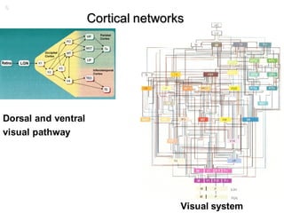
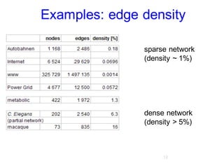
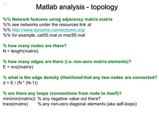
Matlab analysis – spatial organisation
% network with 3D coordinates in variable pos e.g. using
% http://www.dynamic-connectome.org/t/tutorial/honey.mat
%% visualize network
spy(matrix) % binary view
pcolor(matrix) % view of values for weighted networks
hist(nonzeros(matrix))
unique(nonzeros(matrix))
%% Spatial Network visualisation
% view from top
subplot(1,3,1); gplot(pos(:, [1,2])); axis equal
% view from side
subplot(1,3,2); gplot(pos(:, [1,3])); axis equal
% view from back
subplot(1,3,3); gplot(pos(:, [2,3])); axis equal](https://image.slidesharecdn.com/kaiser1-160718102105/85/A-tutorial-in-Connectome-Analysis-1-Marcus-Kaiser-29-320.jpg)

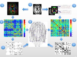
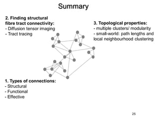
1. Neural networks can be examined at multiple levels from individual axons between neurons to fibre tracts between brain areas. 2. Types of connectivity include structural revealed by DTI, functional from correlated activity, and effective showing causal relationships. 3. Network analysis examines topological properties like modular clusters, small-world organization with high clustering and short path lengths, as well as spatial organization of brain regions.


![Polymer [ बहुलक ] Chemistry Notes PDF - Irfanullah Mehar - JJ Sir Chemistry.pdf](https://cdn.slidesharecdn.com/ss_thumbnails/polymerchemistrynotespdf-irfanullahmehar-jjsirchemistry-260210172118-3f9b37f7-thumbnail.jpg?width=640&height=640&fit=bounds)
