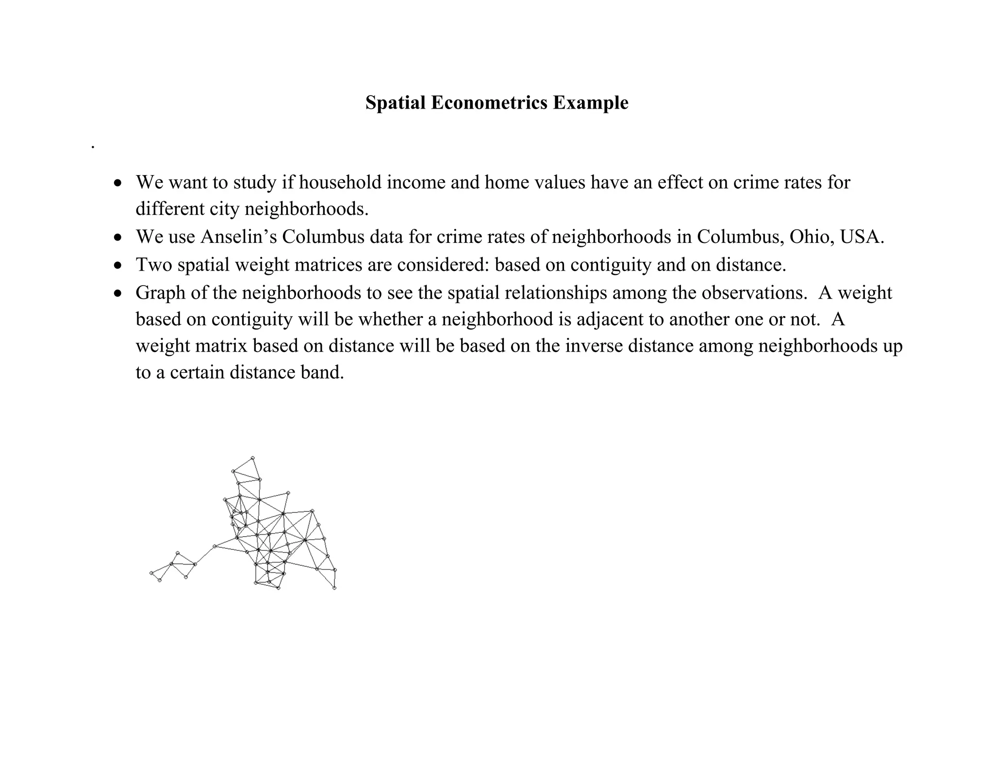
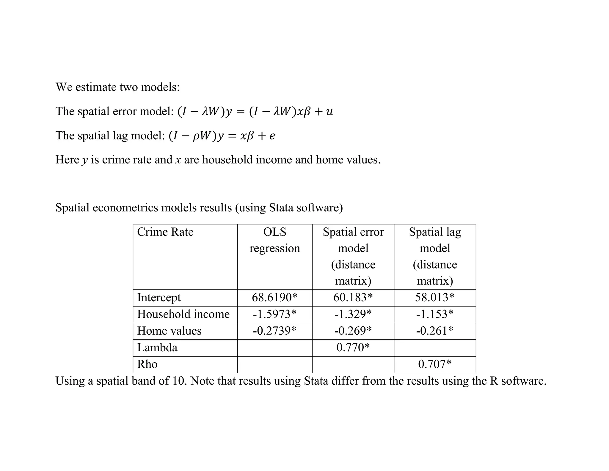
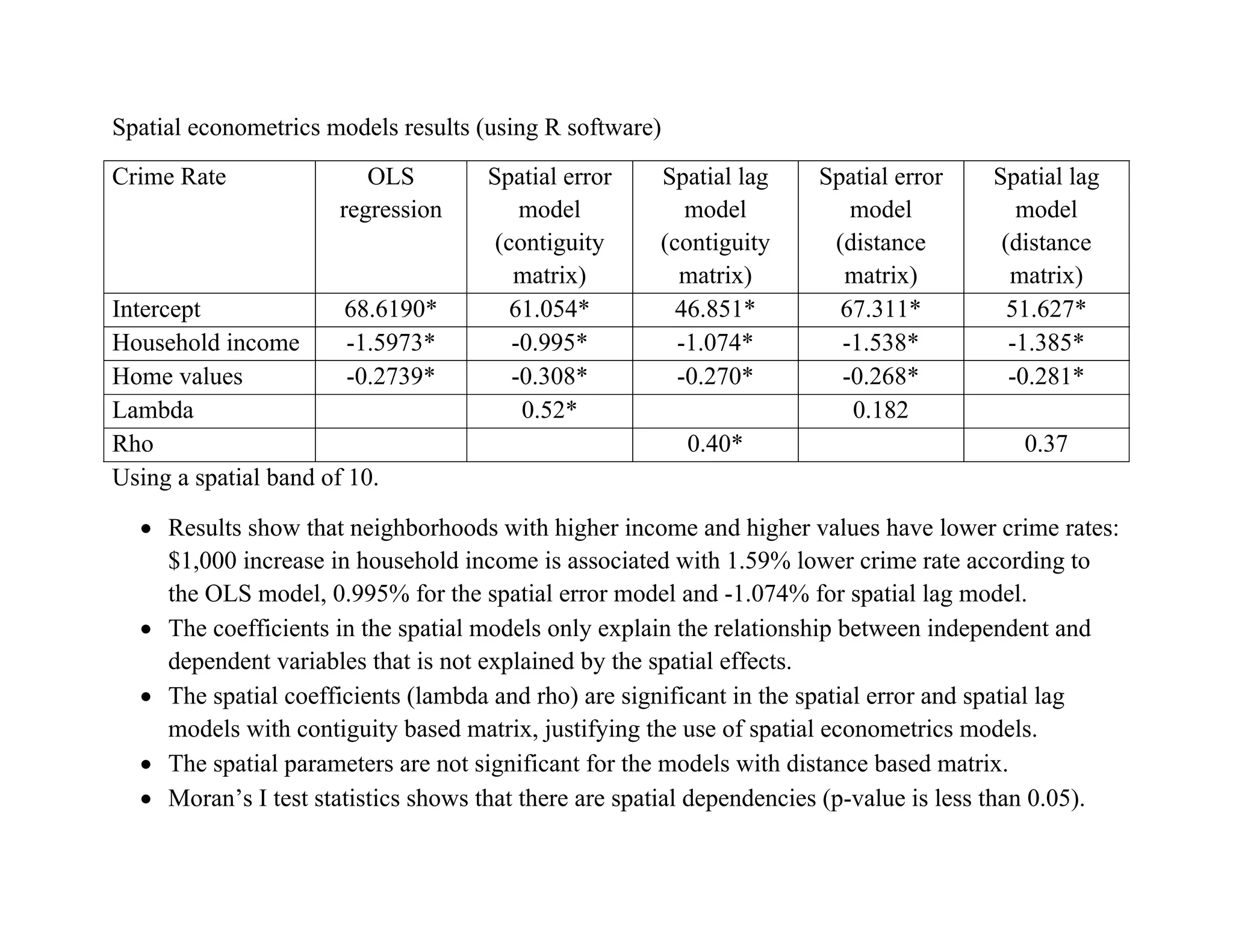
The document analyzes the effects of household income and home values on crime rates across neighborhoods in Columbus, Ohio using spatial econometric models. It estimates spatial error and spatial lag models using two different spatial weight matrices based on contiguity and distance. The results show that higher income and home values are associated with lower crime rates. The spatial coefficients are significant for models using the contiguity matrix, indicating the need to account for spatial effects, but are not significant for models using the distance matrix.

1. Spatial Econometrics Example
Ani Katchova
© 2013 by Ani Katchova. All rights reserved.

2. Spatial Econometrics Example
.
 We want to study if household income and home values have an effect on crime rates for
different city neighborhoods.
 We use Anselin’s Columbus data for crime rates of neighborhoods in Columbus, Ohio, USA.
 Two spatial weight matrices are considered: based on contiguity and on distance.
 Graph of the neighborhoods to see the spatial relationships among the observations. A weight
based on contiguity will be whether a neighborhood is adjacent to another one or not. A
weight matrix based on distance will be based on the inverse distance among neighborhoods up
to a certain distance band.

3. We estimate two models:
The spatial error model:
The spatial lag model:
Here y is crime rate and x are household income and home values.
Spatial econometrics models results (using Stata software)
Crime Rate OLS
regression
Spatial error
model
(distance
matrix)
Spatial lag
model
(distance
matrix)
Intercept 68.6190* 60.183* 58.013*
Household income -1.5973* -1.329* -1.153*
Home values -0.2739* -0.269* -0.261*
Lambda 0.770*
Rho 0.707*
Using a spatial band of 10. Note that results using Stata differ from the results using the R software.

4. Spatial econometrics models results (using R software)
Crime Rate OLS
regression
Spatial error
model
(contiguity
matrix)
Spatial lag
model
(contiguity
matrix)
Spatial error
model
(distance
matrix)
Spatial lag
model
(distance
matrix)
Intercept 68.6190* 61.054* 46.851* 67.311* 51.627*
Household income -1.5973* -0.995* -1.074* -1.538* -1.385*
Home values -0.2739* -0.308* -0.270* -0.268* -0.281*
Lambda 0.52* 0.182
Rho 0.40* 0.37
Using a spatial band of 10.
 Results show that neighborhoods with higher income and higher values have lower crime rates:
$1,000 increase in household income is associated with 1.59% lower crime rate according to
the OLS model, 0.995% for the spatial error model and -1.074% for spatial lag model.
 The coefficients in the spatial models only explain the relationship between independent and
dependent variables that is not explained by the spatial effects.
 The spatial coefficients (lambda and rho) are significant in the spatial error and spatial lag
models with contiguity based matrix, justifying the use of spatial econometrics models.
 The spatial parameters are not significant for the models with distance based matrix.
 Moran’s I test statistics shows that there are spatial dependencies (p-value is less than 0.05).

5. Plot of spatial dependent of the dependent variable. The 45 degree line represents perfect prediction
of the dependent variable y by its neighbors (lagged value for the dependent variable Wy). From the
graph it does not look like there is a perfect prediction.