This document provides an introduction to biostatistics. It defines biostatistics as the application of statistics to biology, involving the collection, presentation, analysis, and interpretation of biological data to aid decision-making. The roles of statisticians are to design studies, analyze data using statistical procedures, and present results to researchers. Data can come from records, surveys, or experiments. Data types include quantitative continuous, quantitative discrete, qualitative nominal, and qualitative ordinal variables. Common methods to present data are numerical tables, graphs, and mathematical summaries including measures of central tendency, dispersion, and standard error.

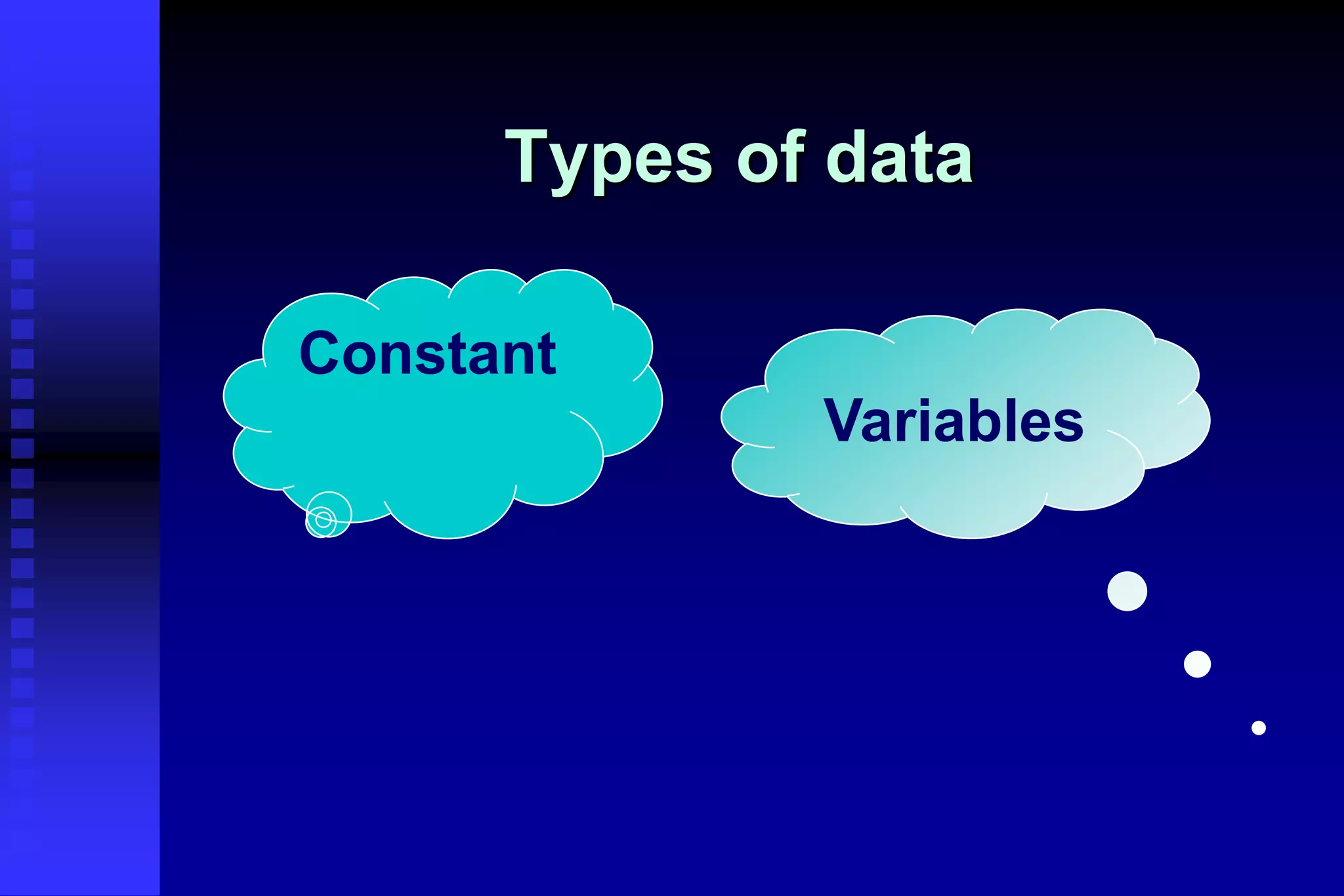
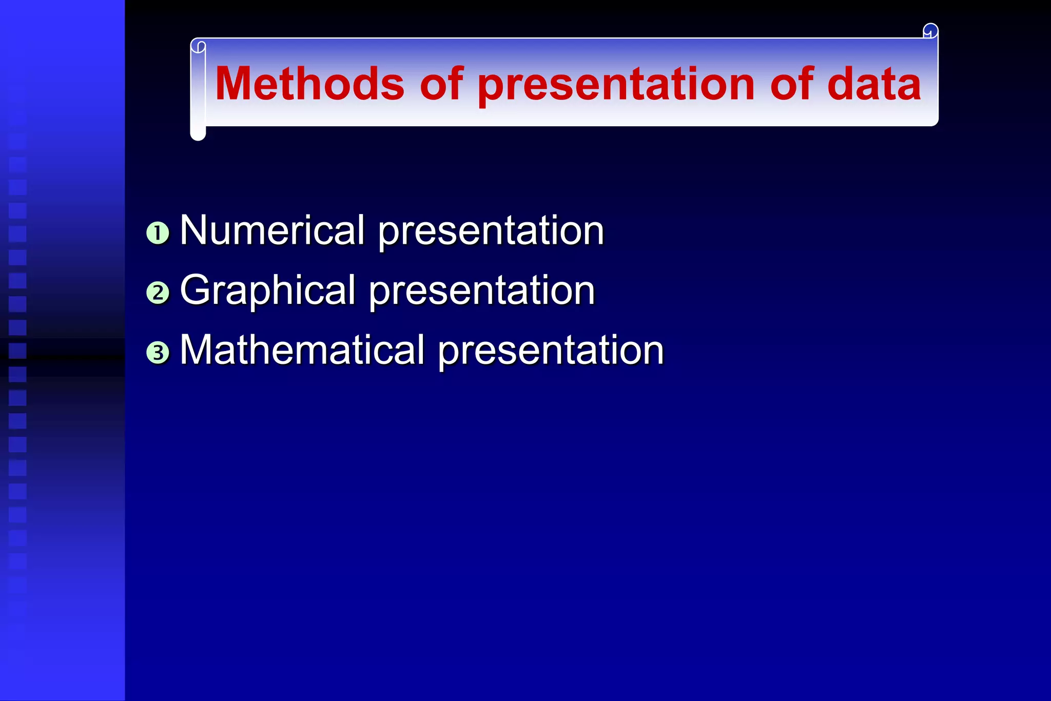
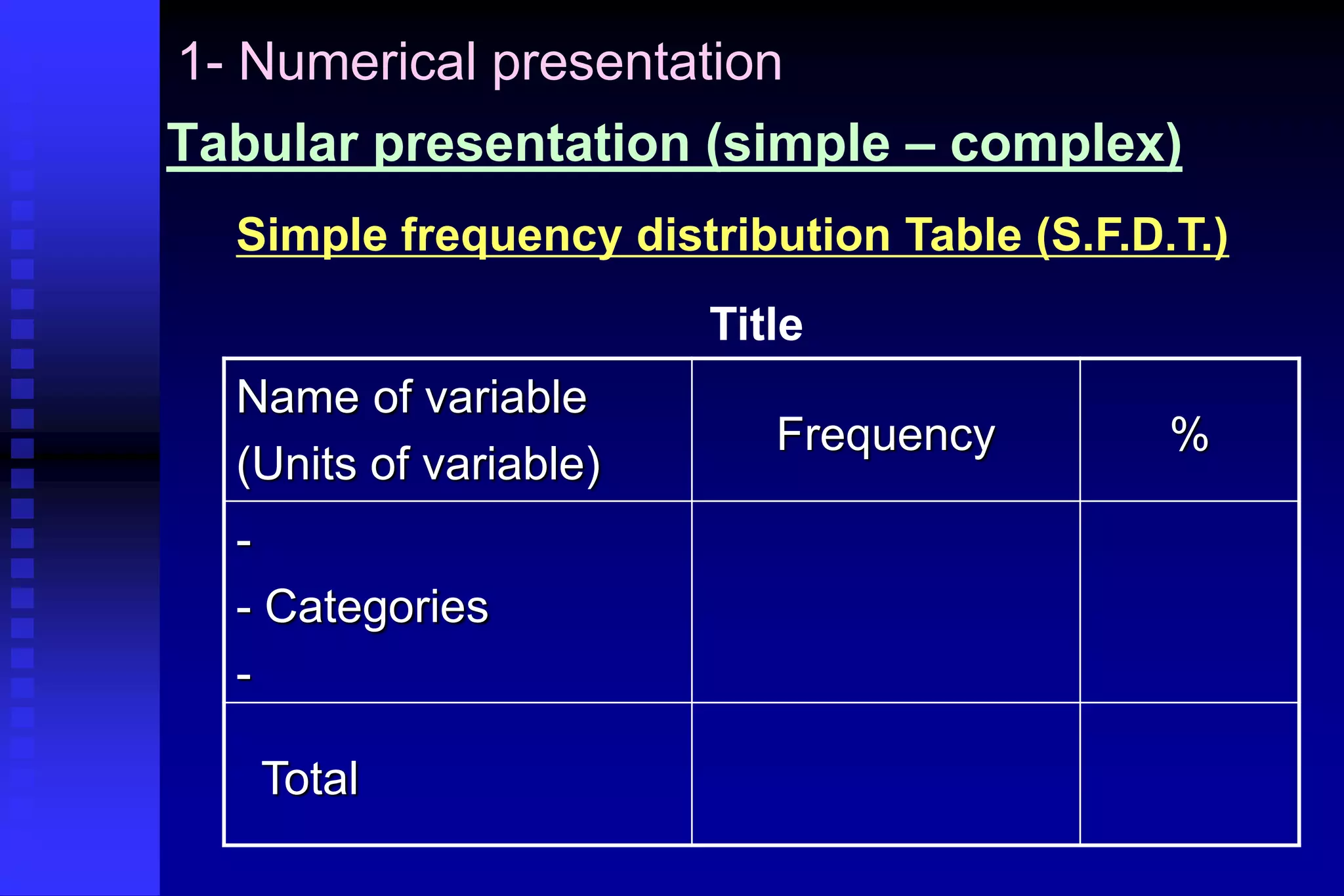
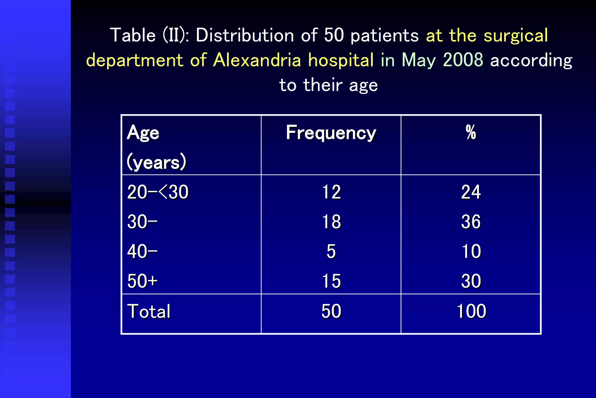
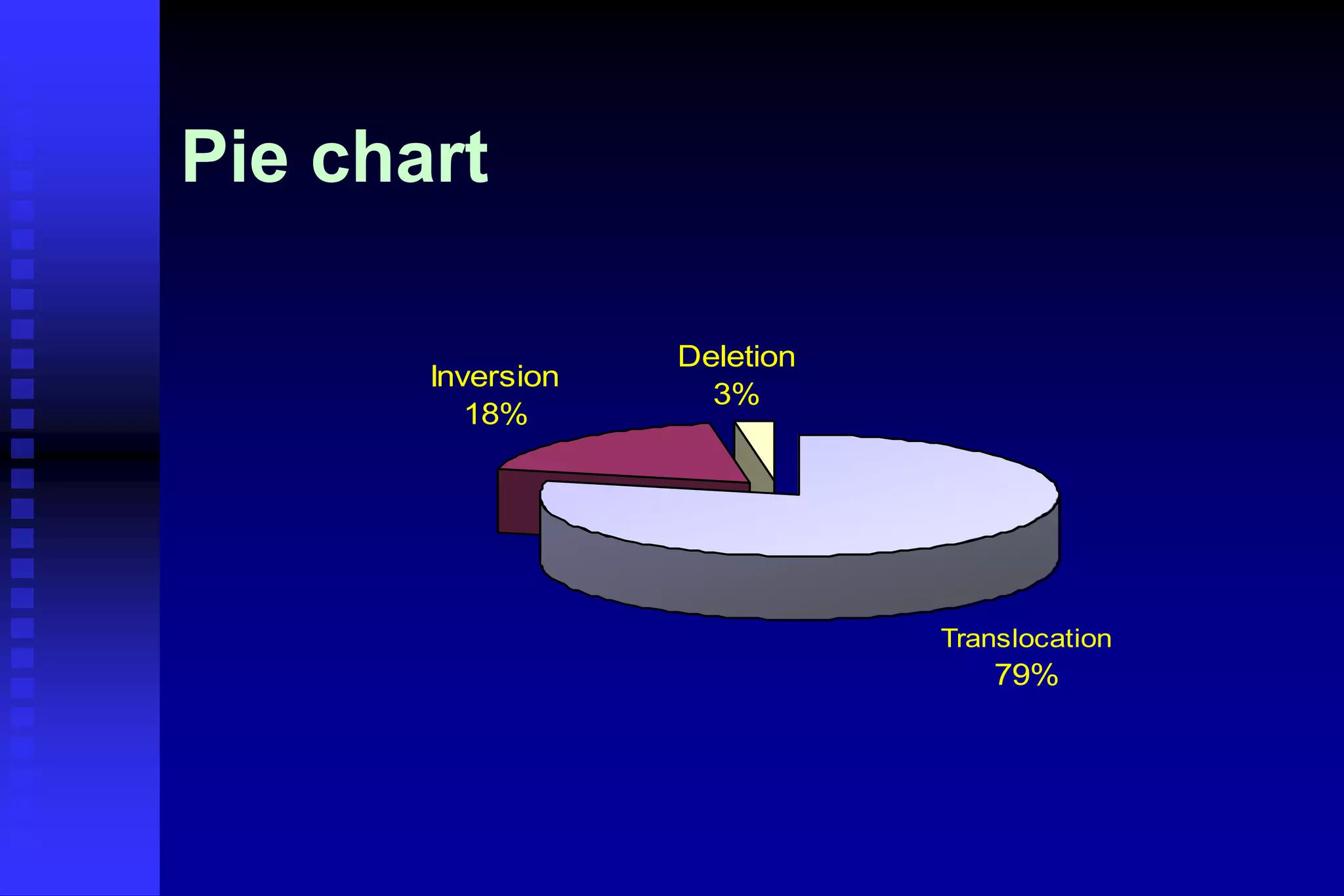
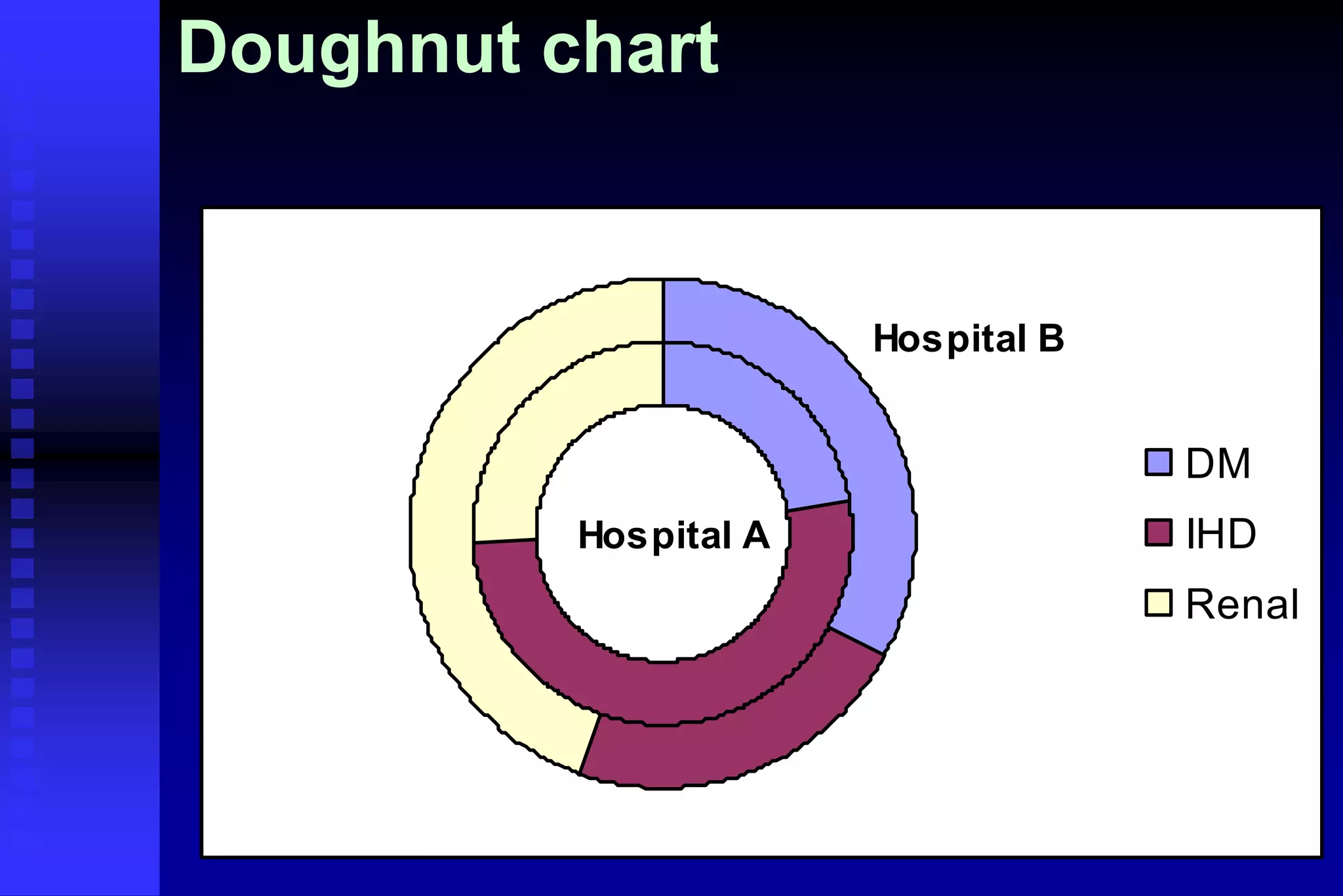
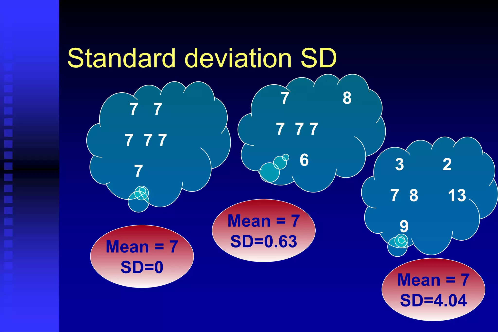
1. ‫الرحيم‬ ‫الرحمن‬ ‫هللا‬ ‫بسم‬

2. Introduction to
Biostatistics
Dr. Moataza Mahmoud Abdel Wahab
Lecturer of Biostatistics
High Institute of Public Health
University of Alexandria

3. Biostatistics
(a portmanteau word made from biology and
statistics)
The application of statistics to a wide range of topics
in biology.

4. Biostatistics
It is the science which deals with development and
application of the most appropriate methods for
the:
Collection of data.
Presentation of the collected data.
Analysis and interpretation of the results.
Making decisions on the basis of such analysis

5. Other definitions for “Statistics”
 Frequently used in referral to recorded data
 Denotes characteristics calculated for a set of data :
sample mean

6. Role of statisticians
 To guide the design of an experiment or survey
prior to data collection
 To analyze data using proper statistical
procedures and techniques
 To present and interpret the results to researchers
and other decision makers

7. Sources of
data
Records Surveys Experiments
Comprehensive Sample

8. Types of data
Constant
Variables

9. Quantitative
continuous
Types of variables
Quantitative variables Qualitative variables
Quantitative
descrete
Qualitative
nominal
Qualitative
ordinal

10.  Numerical presentation
 Graphical presentation
 Mathematical presentation
Methods of presentation of data

11. 1- Numerical presentation
Tabular presentation (simple – complex)
Simple frequency distribution Table (S.F.D.T.)
Title
Name of variable
(Units of variable)
Frequency %
-
- Categories
-
Total

12. Table (I): Distribution of 50 patients at the surgical
department of Alexandria hospital in May 2008 according
to their ABO blood groups
Blood group Frequency %
A
B
AB
O
12
18
5
15
24
36
10
30
Total 50 100

13. Table (II): Distribution of 50 patients at the surgical
department of Alexandria hospital in May 2008 according
to their age
Age
(years)
Frequency %
20-<30
30-
40-
50+
12
18
5
15
24
36
10
30
Total 50 100

14. Complex frequency distribution Table
Table (III): Distribution of 20 lung cancer patients at the chest department
of Alexandria hospital and 40 controls in May 2008 according to smoking
Smoking
Lung cancer
Total
Cases Control
No. % No. % No. %
Smoker 15 75% 8 20% 23 38.33
Non
smoker 5 25% 32 80% 37 61.67
Total 20 100 40 100 60 100

15. Complex frequency distribution Table
Table (IV): Distribution of 60 patients at the chest department of
Alexandria hospital in May 2008 according to smoking & lung cancer
Smoking
Lung cancer
Total
positive negative
No. % No. % No. %
Smoker 15 65.2 8 34.8 23 100
Non
smoker 5 13.5 32 86.5 37 100
Total 20 33.3 40 66.7 60 100

16. 2- Graphical presentation
 Graphs drawn using Cartesian
coordinates
• Line graph
• Frequency polygon
• Frequency curve
• Histogram
• Bar graph
• Scatter plot
 Pie chart
 Statistical maps
rules

17. Line Graph
0
10
20
30
40
50
60
1960 1970 1980 1990 2000
Year
MMR/1000 Year MMR
1960 50
1970 45
1980 26
1990 15
2000 12
Figure (1): Maternal mortality rate of
(country), 1960-2000

18. Frequency polygon
Age
(years)
Sex Mid-point of interval
Males Females
20 - 3 (12%) 2 (10%) (20+30) / 2 = 25
30 - 9 (36%) 6 (30%) (30+40) / 2 = 35
40- 7 (8%) 5 (25%) (40+50) / 2 = 45
50 - 4 (16%) 3 (15%) (50+60) / 2 = 55
60 - 70 2 (8%) 4 (20%) (60+70) / 2 = 65
Total 25(100%) 20(100%)

19. Frequency polygon
Age
Sex
M-P
M F
20- (12%) (10%) 25
30- (36%) (30%) 35
40- (8%) (25%) 45
50- (16%) (15%) 55
60-70 (8%) (20%) 65
0
5
10
15
20
25
30
35
40
25 35 45 55 65
Age
%
Males Females
Figure (2): Distribution of 45 patients at (place) , in
(time) by age and sex

20. 0
1
2
3
4
5
6
7
8
9
20- 30- 40- 50- 60-69
Age in years
Frequency
Female
Male
Frequency curve

21. Histogram
Distribution of a group of cholera patients by age
Age (years) Frequency %
25-
30-
40-
45-
60-65
3
5
7
4
2
14.3
23.8
33.3
19.0
9.5
Total 21 100
0
5
10
15
20
25
30
35
0
2
5
3
0
4
0
4
5
6
0
6
5
Age (years)
%
Figure (2): Distribution of 100 cholera patients at (place) , in (time)
by age

22. Bar chart
0
5
10
15
20
25
30
35
40
45
%
Single Married Divorced Widowed
Marital status

23. Bar chart
0
10
20
30
40
50
%
Single Married Divorced Widowed
Marital status
Male
Female

24. Pie chart
Deletion
3%
Inversion
18%
Translocation
79%

25. Doughnut chart
Hospital A
Hospital B
DM
IHD
Renal

26. 3-Mathematical presentation
Summery statistics
Measures of location
1- Measures of central tendency
2- Measures of non central locations
(Quartiles, Percentiles )
Measures of dispersion

27. 1- Measures of central tendency (averages)
Midrange
Smallest observation + Largest observation
2
Mode
the value which occurs with the greatest
frequency i.e. the most common value
Summery statistics

28. 1- Measures of central tendency (cont.)
 Median
the observation which lies in the middle of
the ordered observation.
 Arithmetic mean (mean)
Sum of all observations
Number of observations
Summery statistics

29. Measures of dispersion
 Range
 Variance
 Standard deviation
 Semi-interquartile range
 Coefficient of variation
 “Standard error”

30. Standard deviation SD
7 7
7 7 7
7
7 8
7 7 7
6 3 2
7 8 13
9
Mean = 7
SD=0
Mean = 7
SD=0.63
Mean = 7
SD=4.04

31. Standard error of mean SE
A measure of variability among means of samples
selected from certain population
SE (Mean) =
S
n