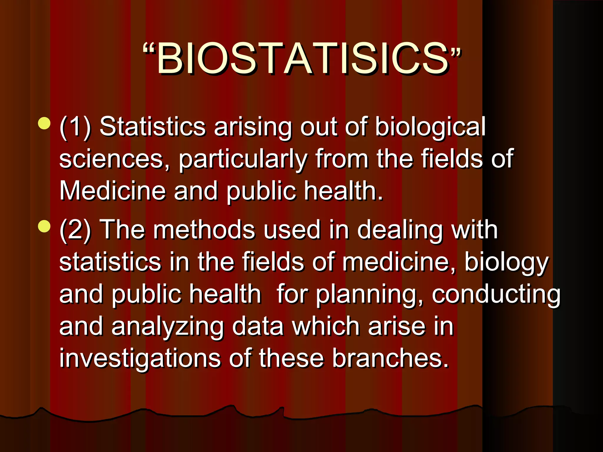
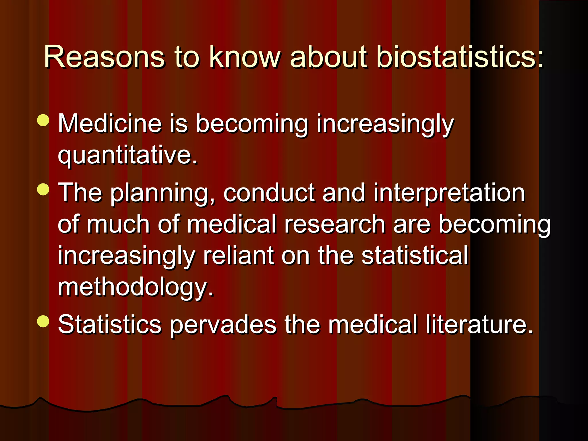
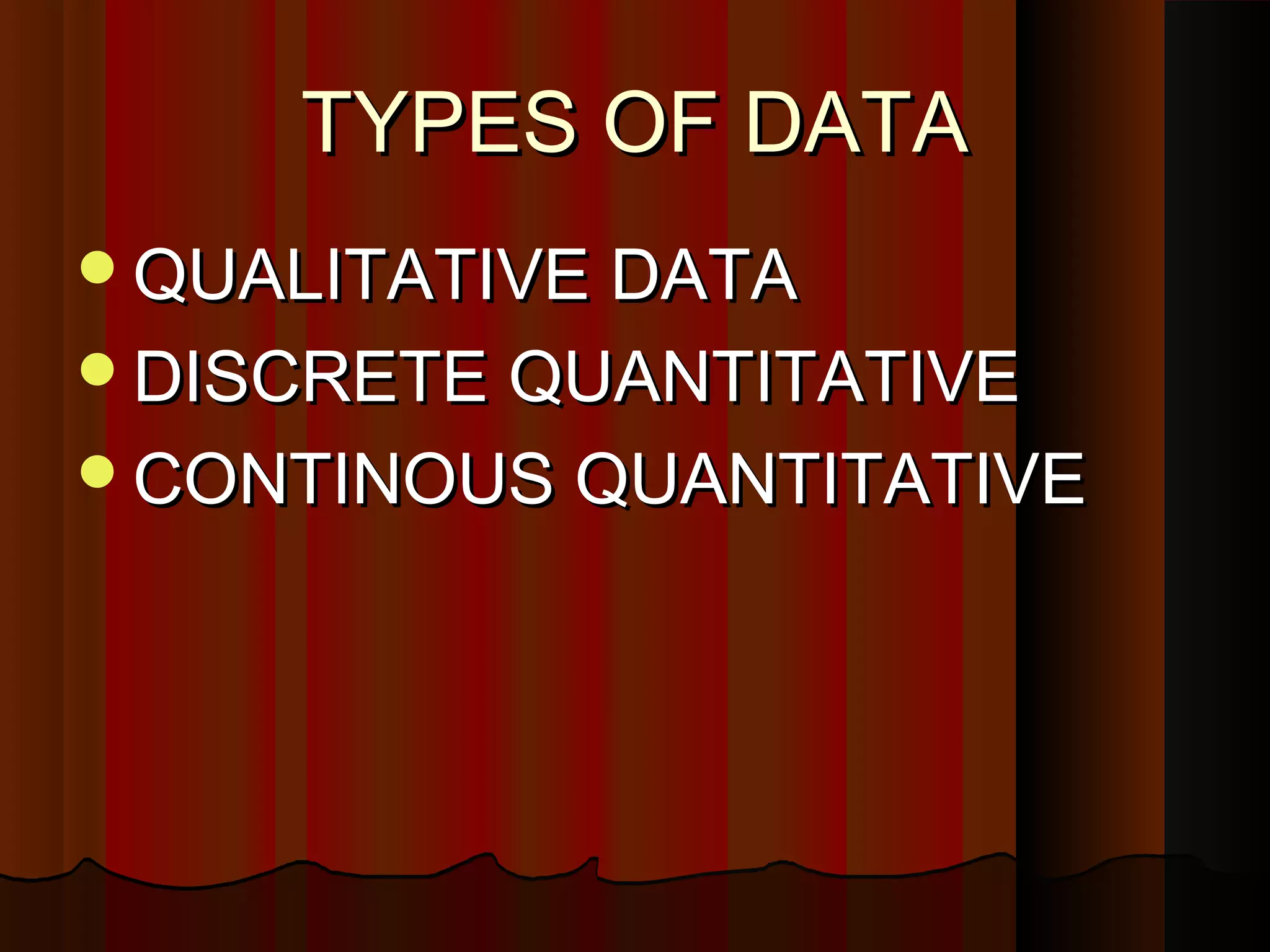
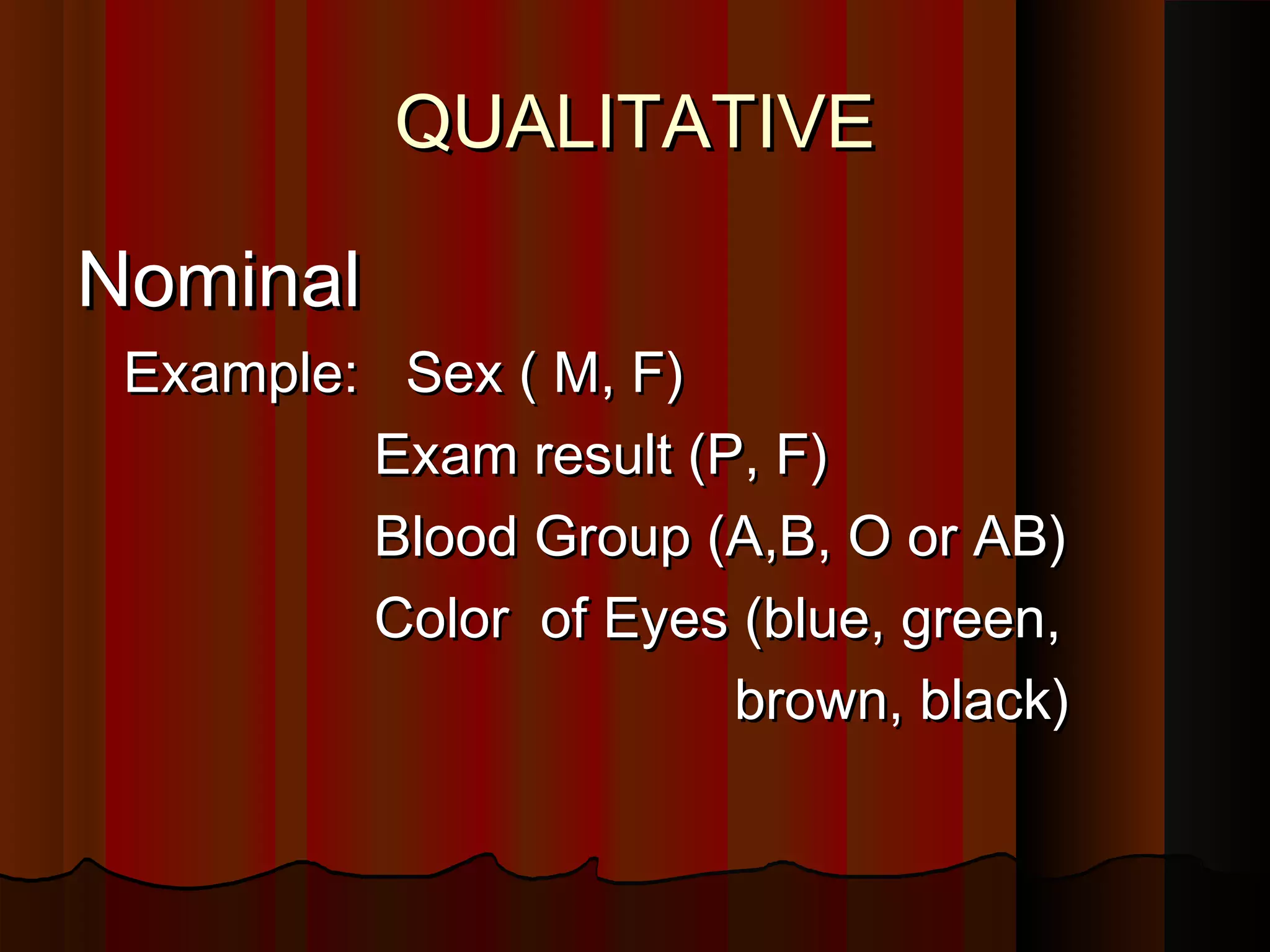
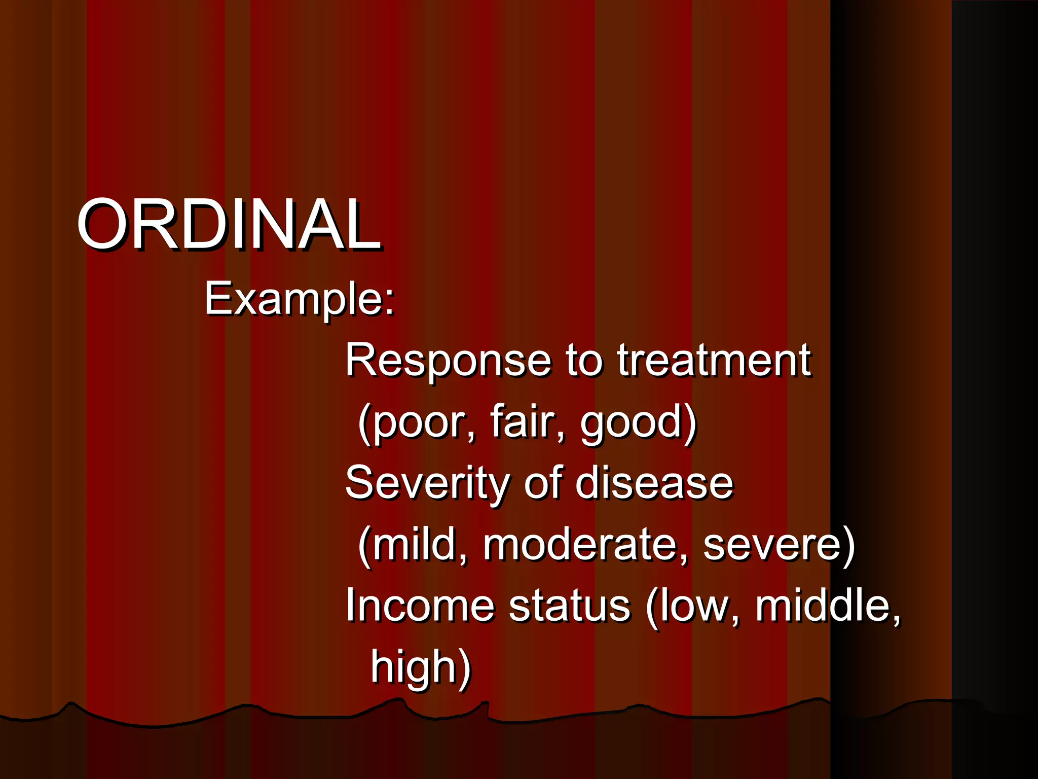
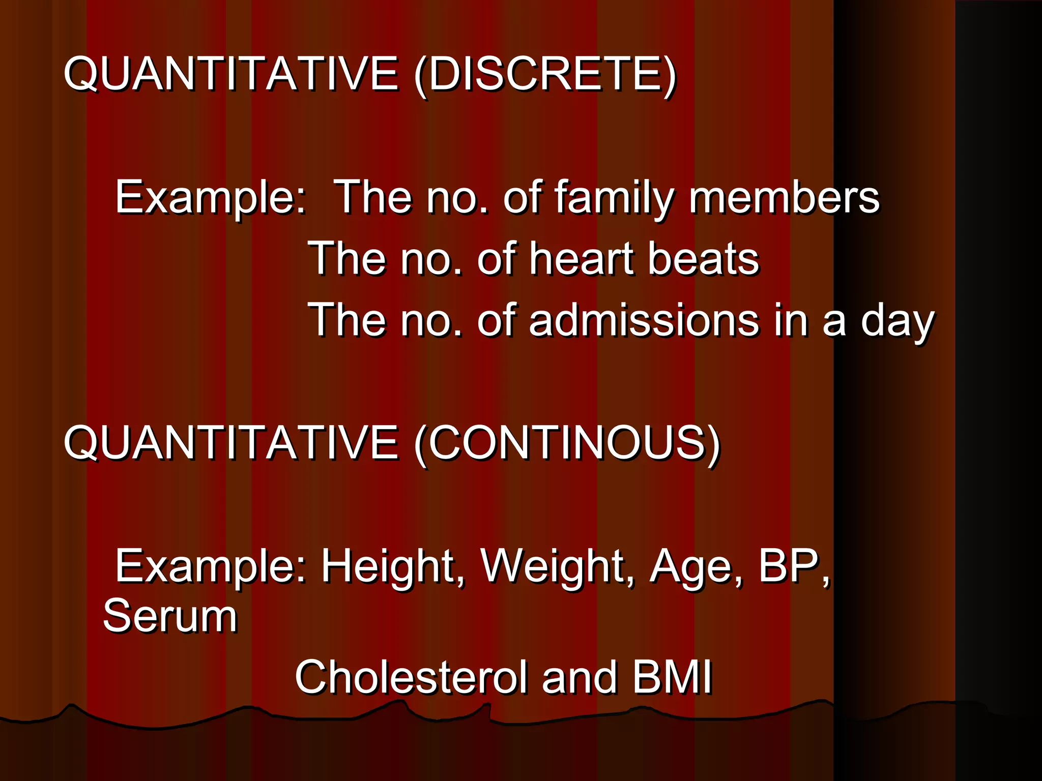
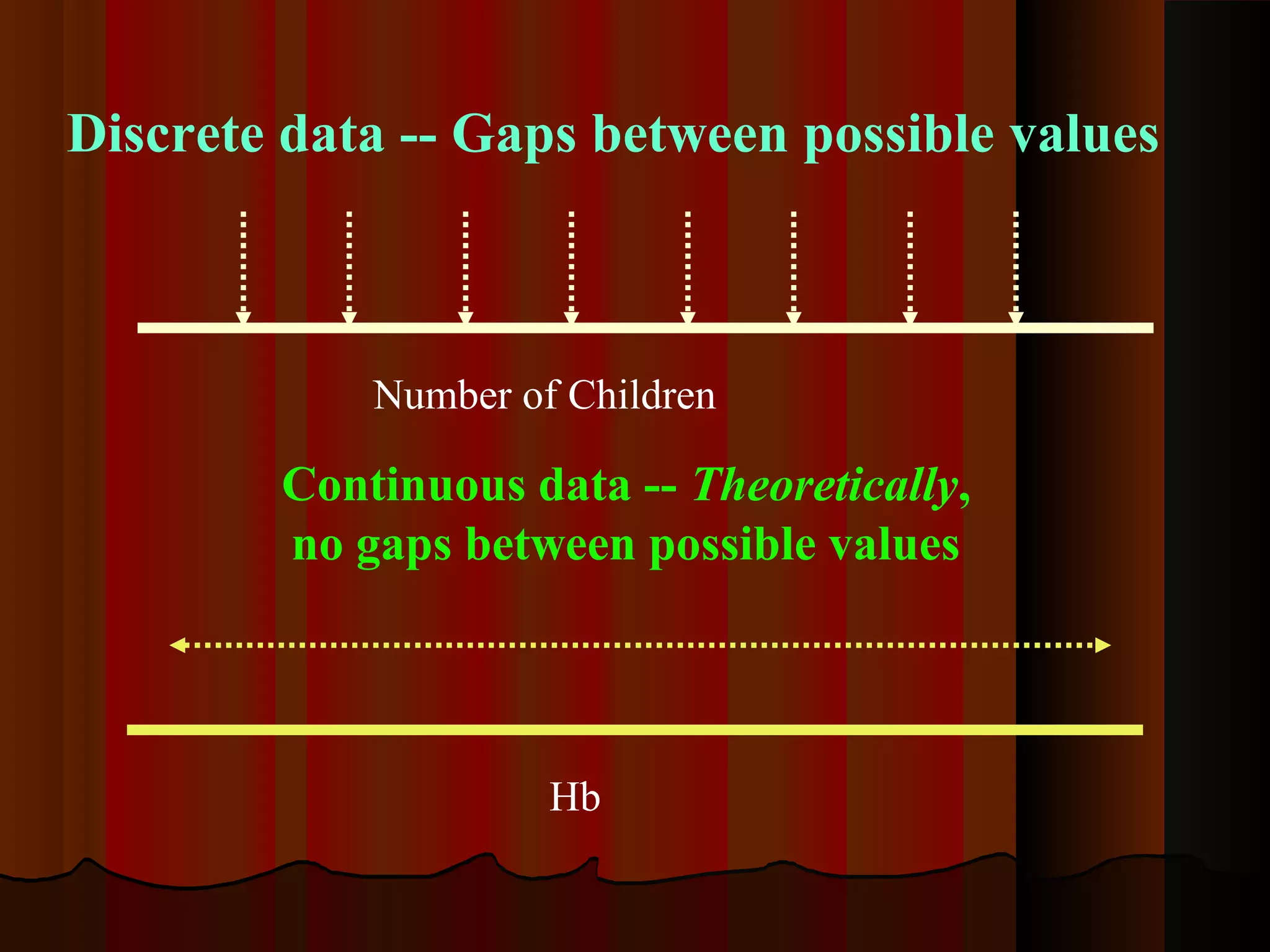
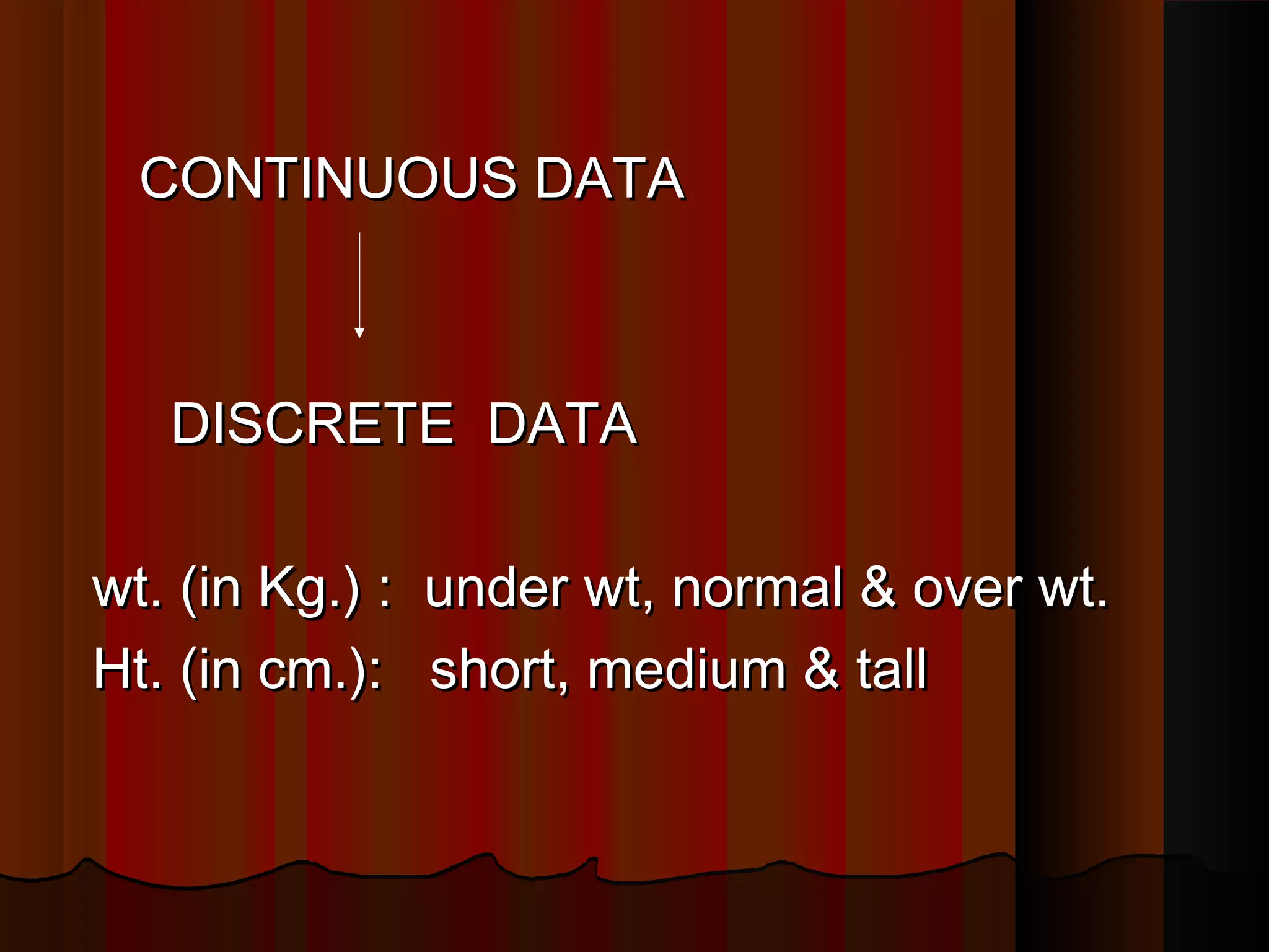
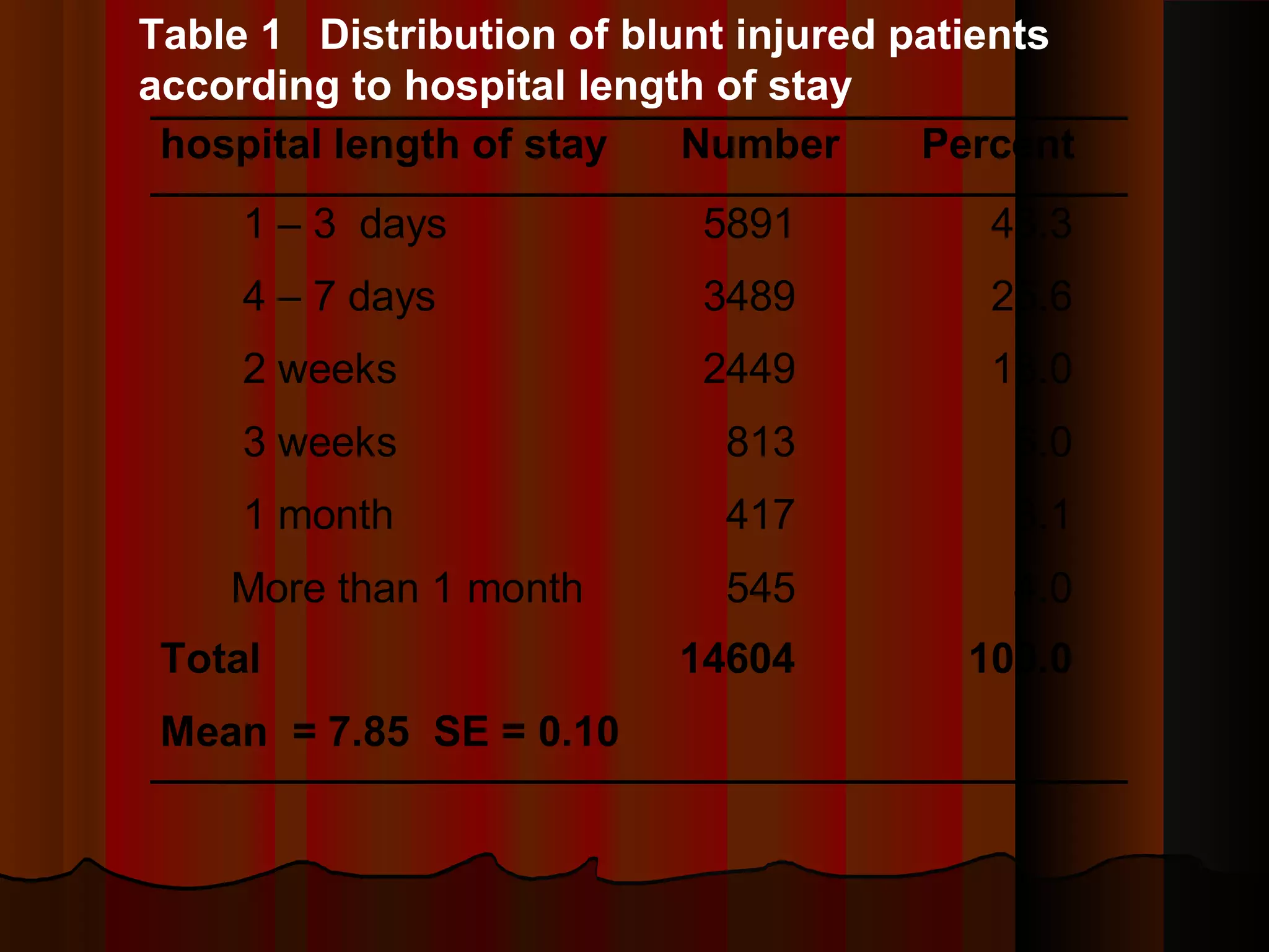
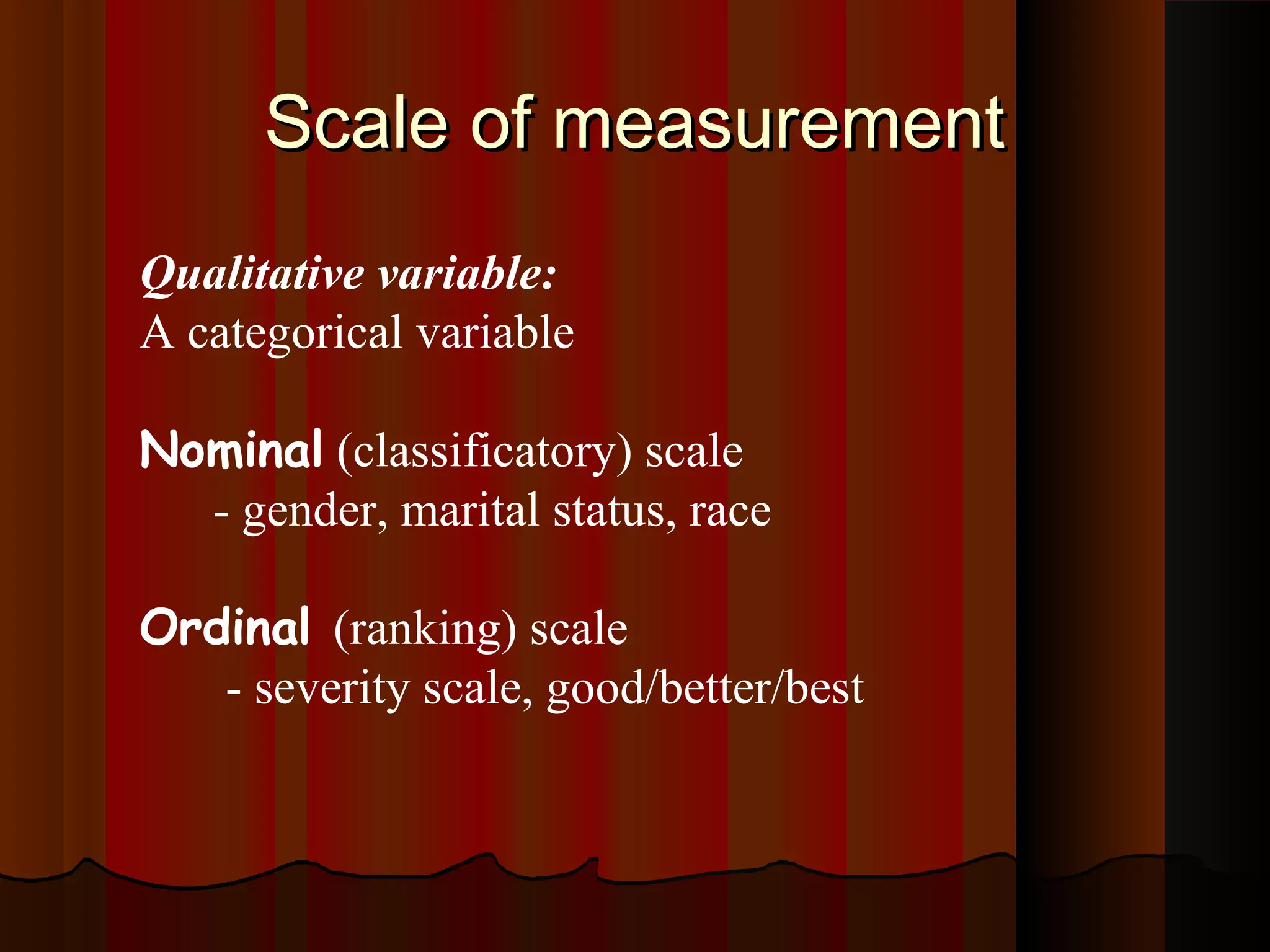
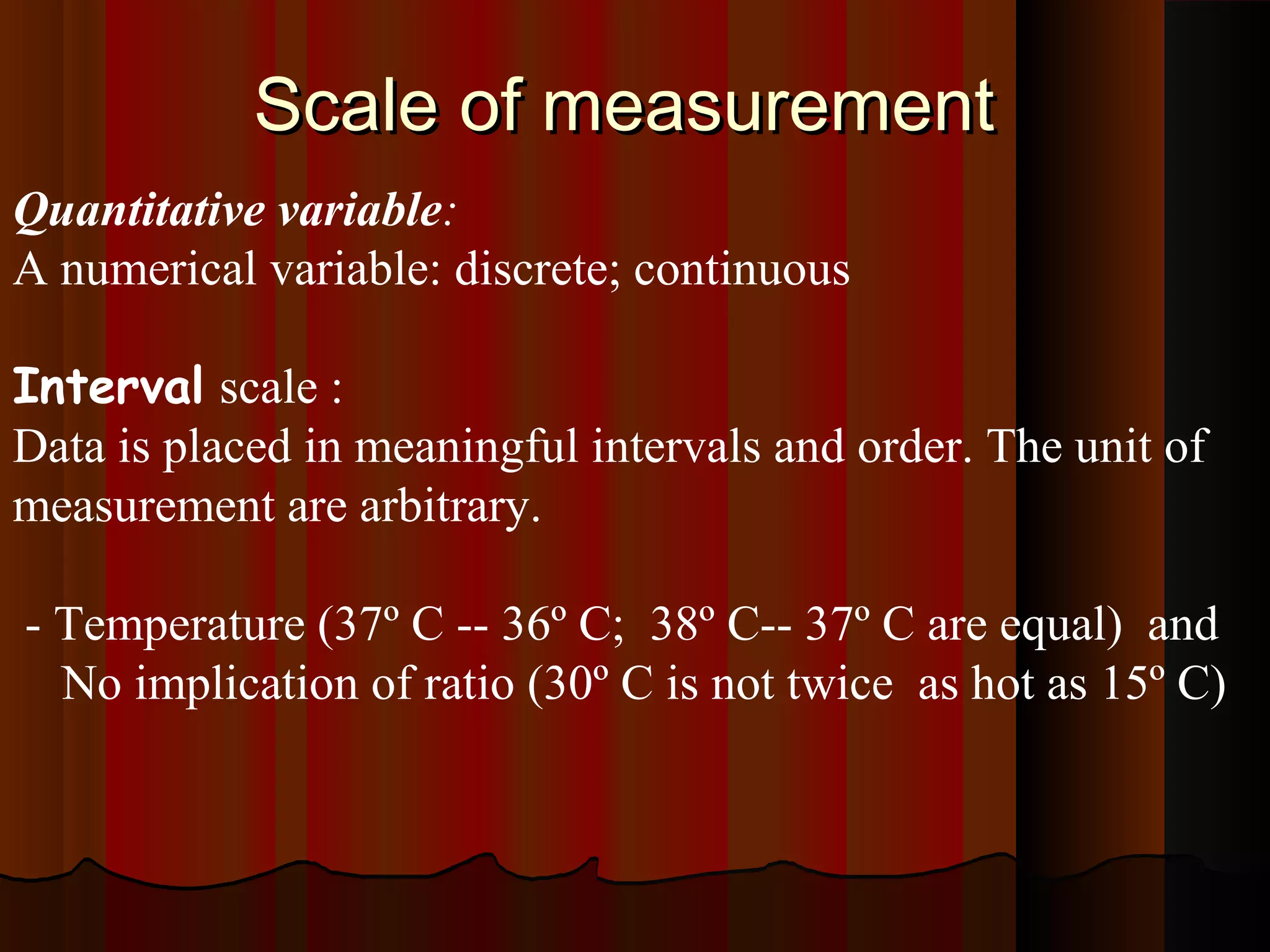
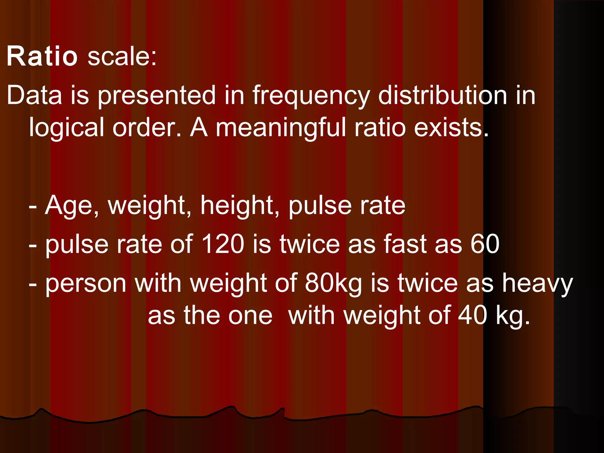
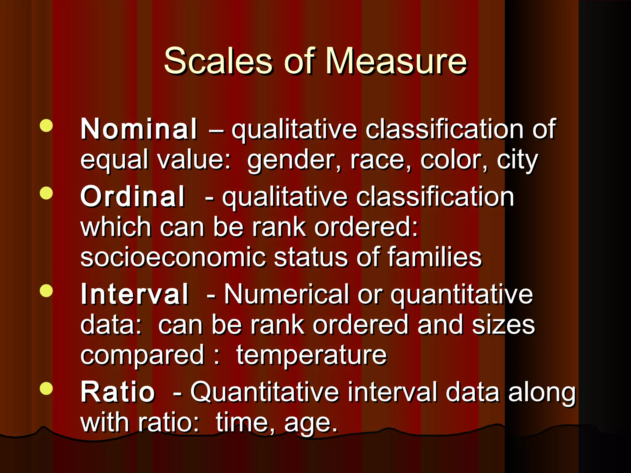
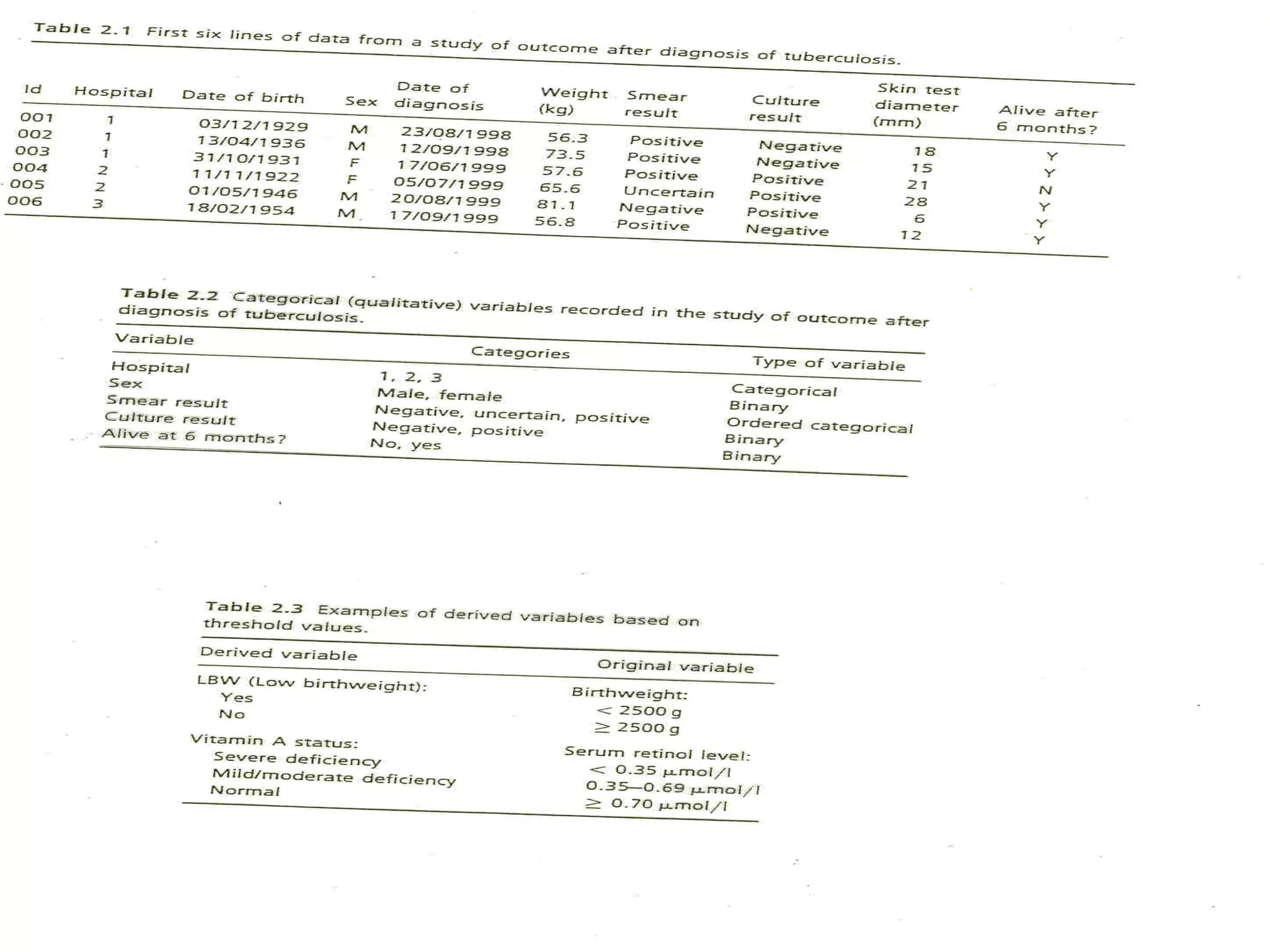
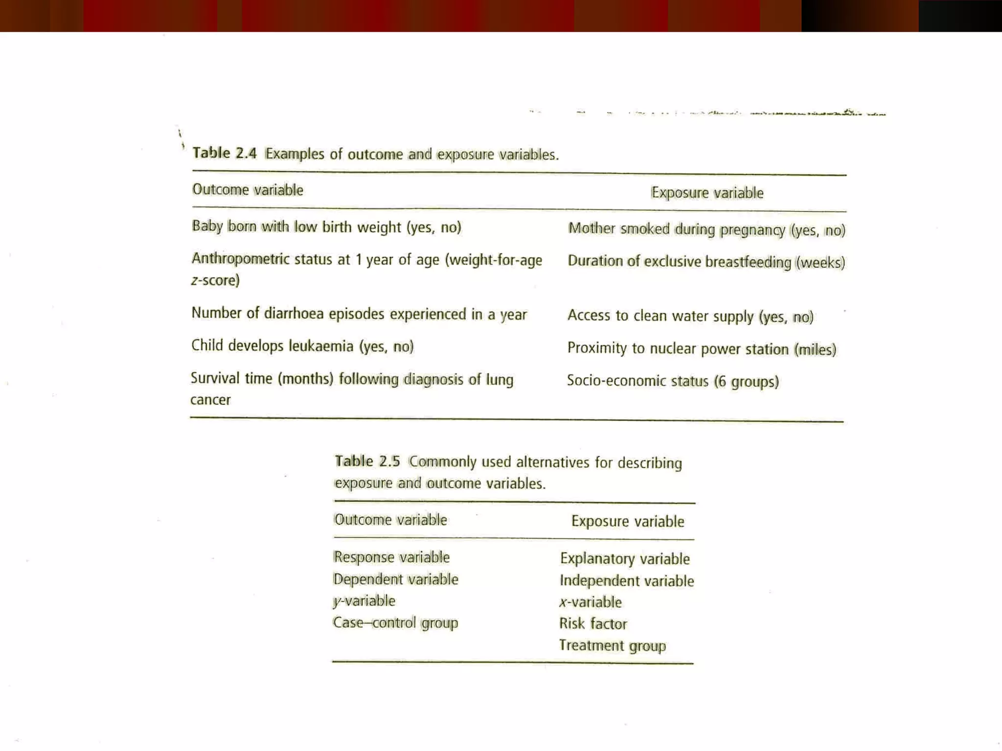
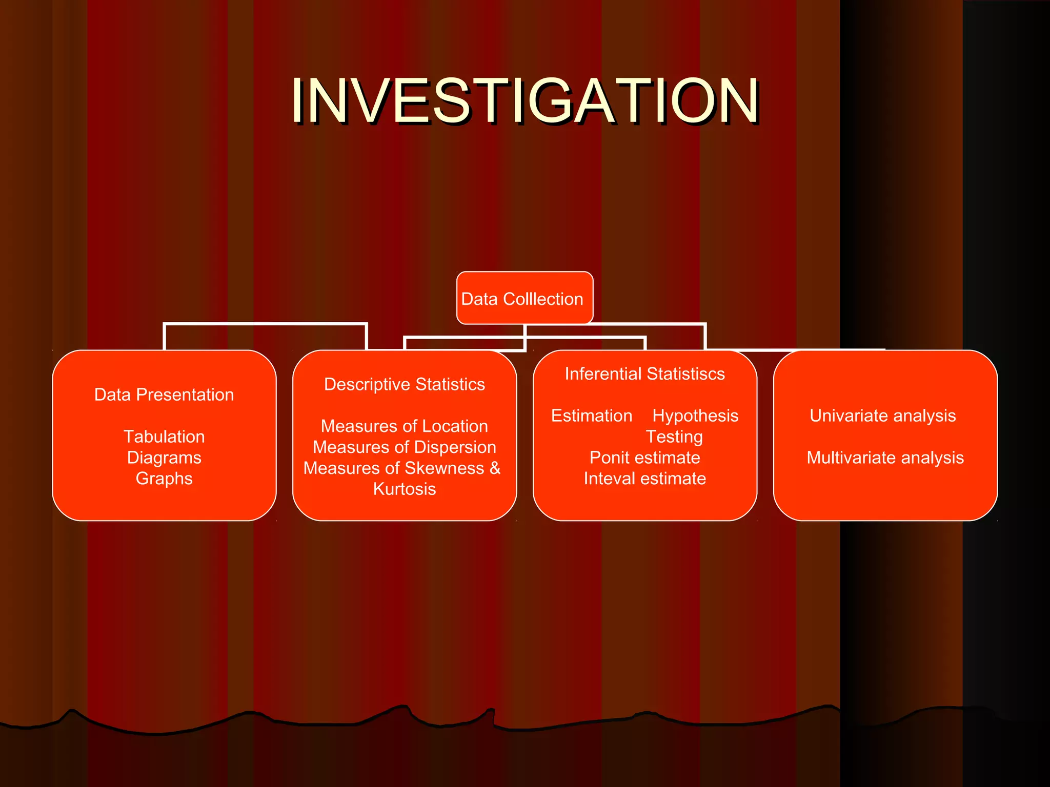
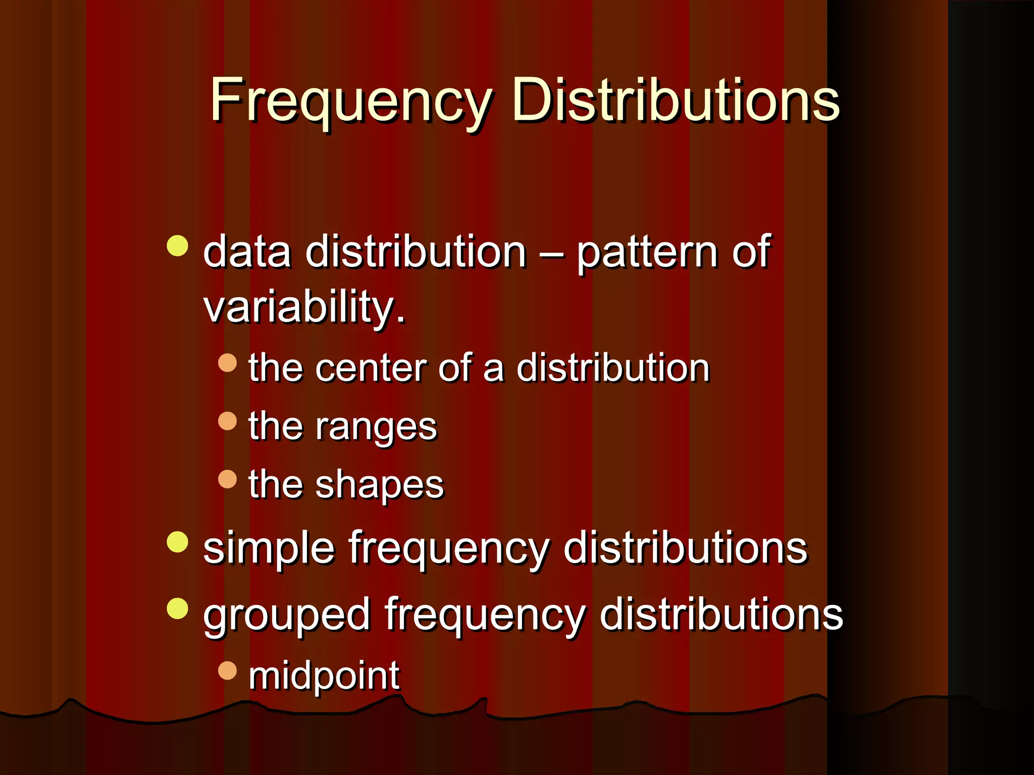
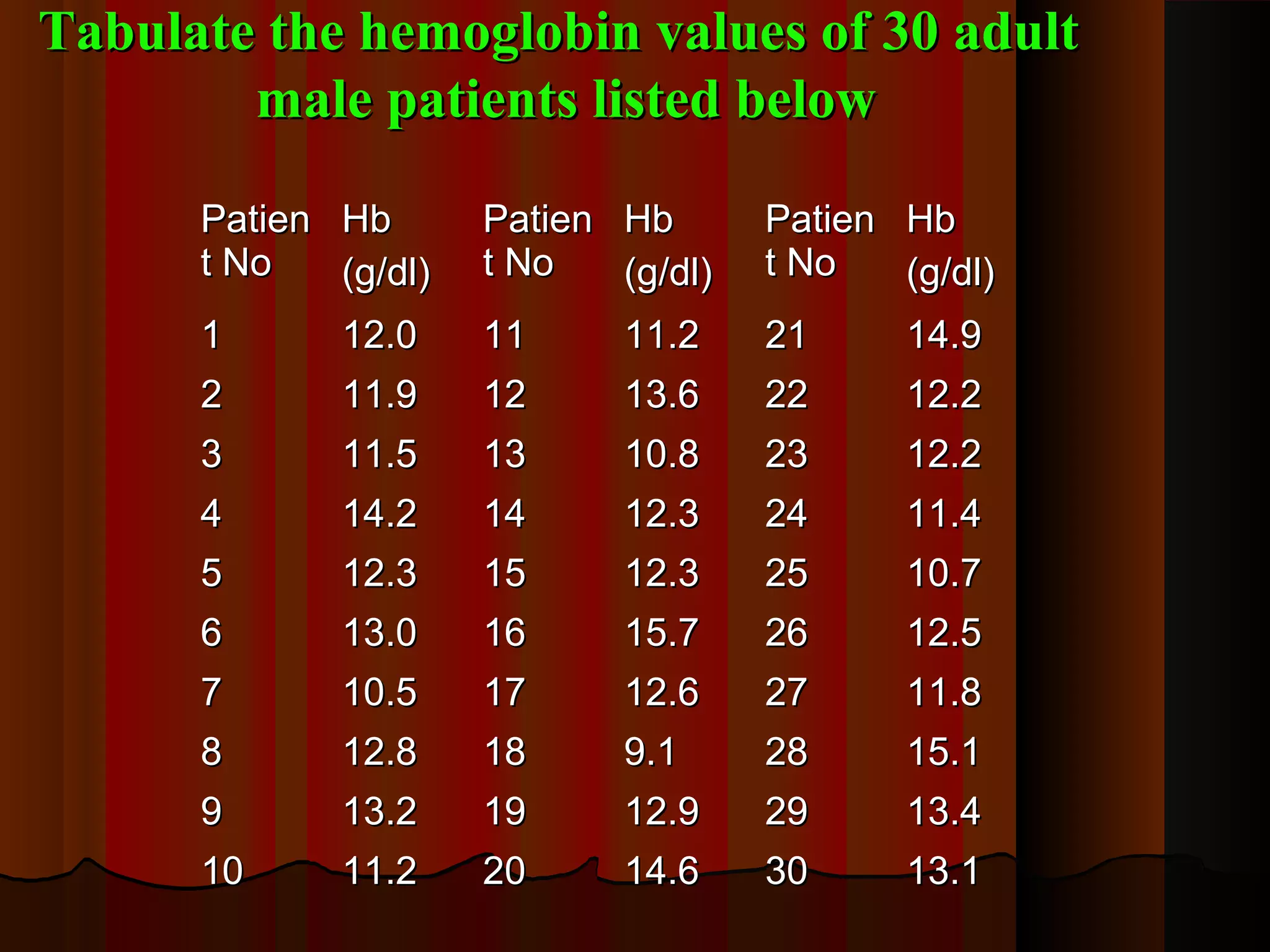
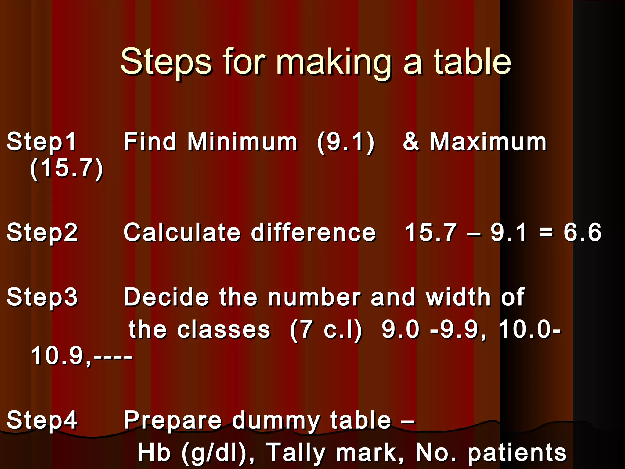
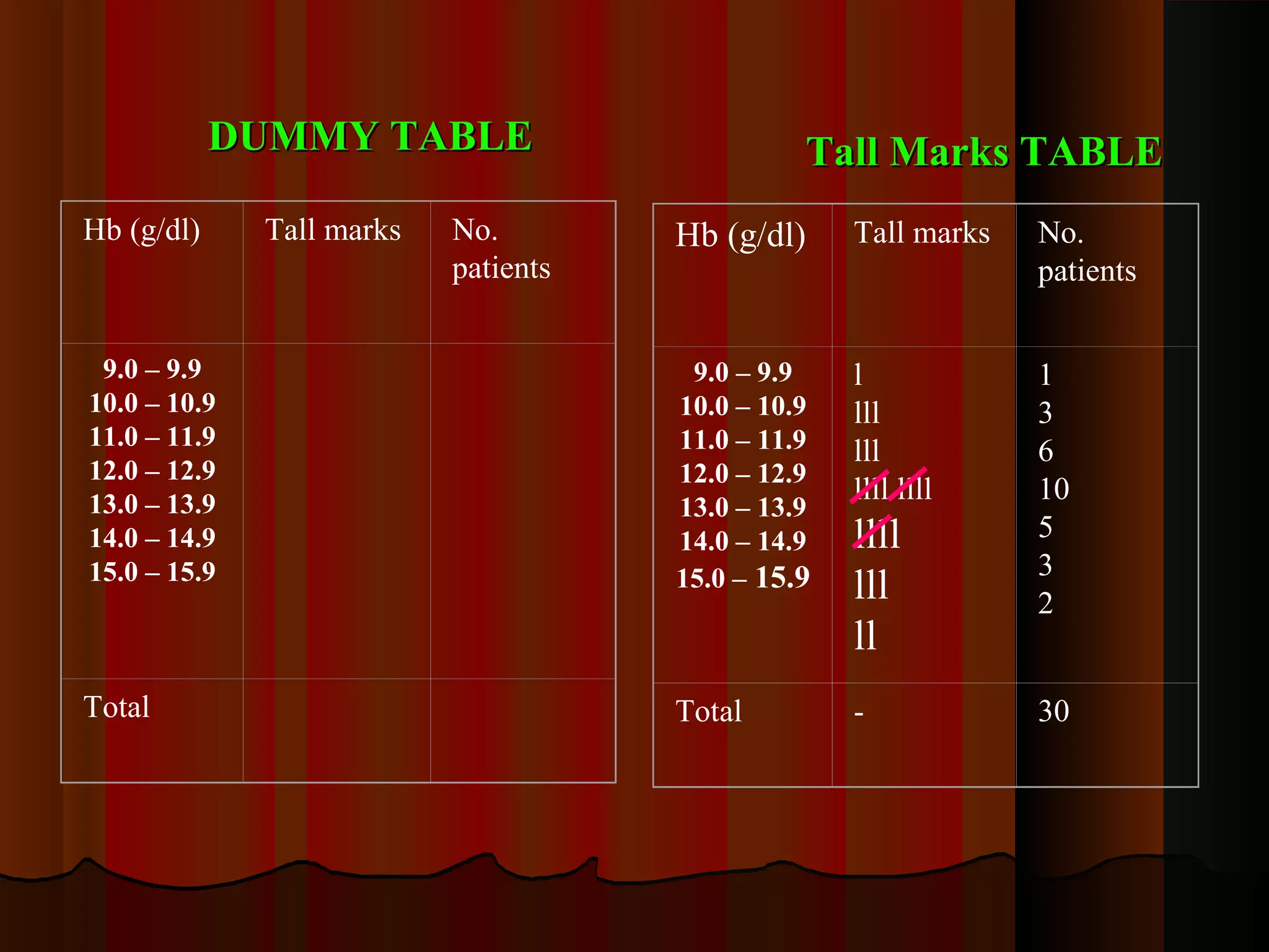
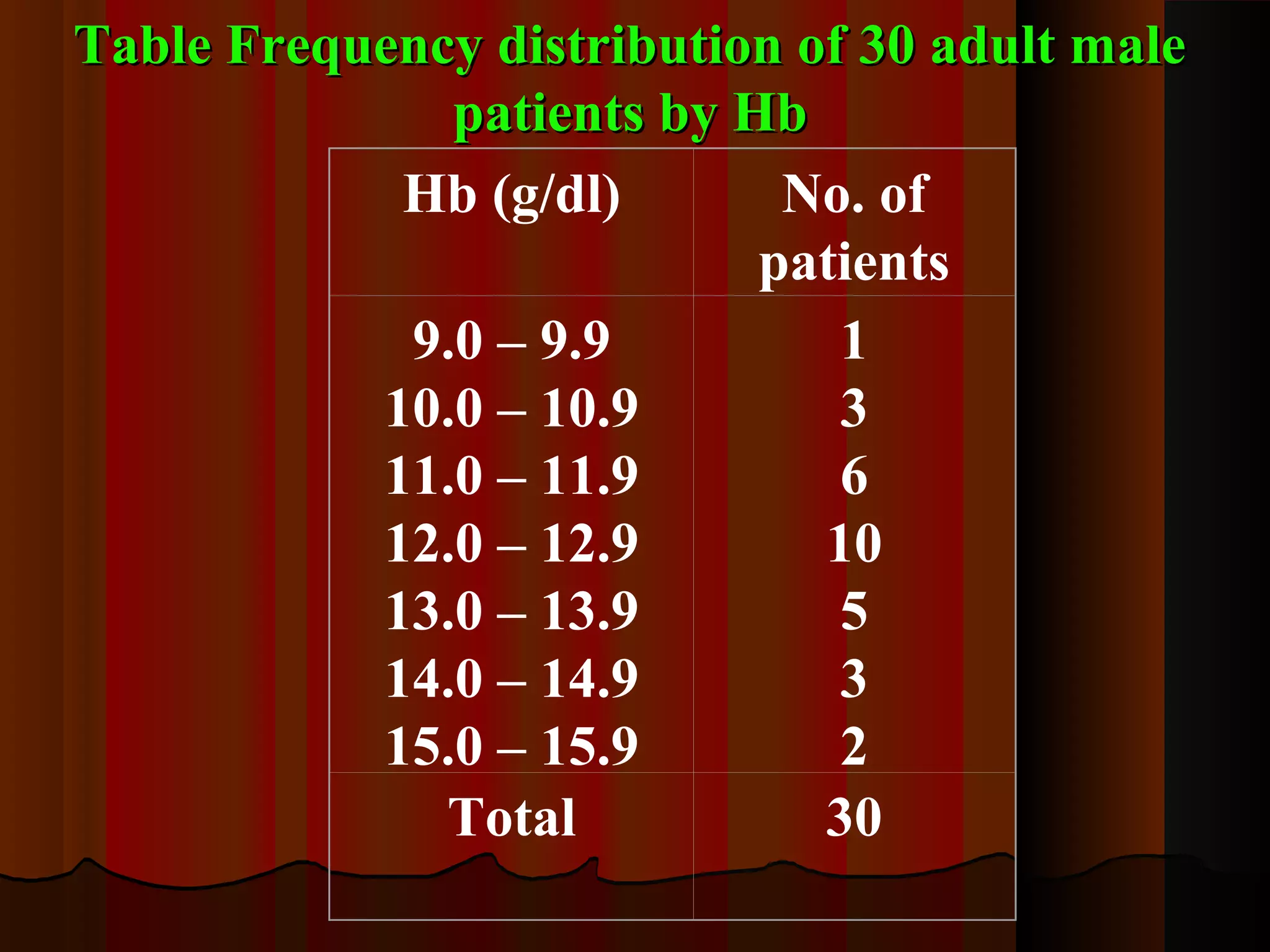
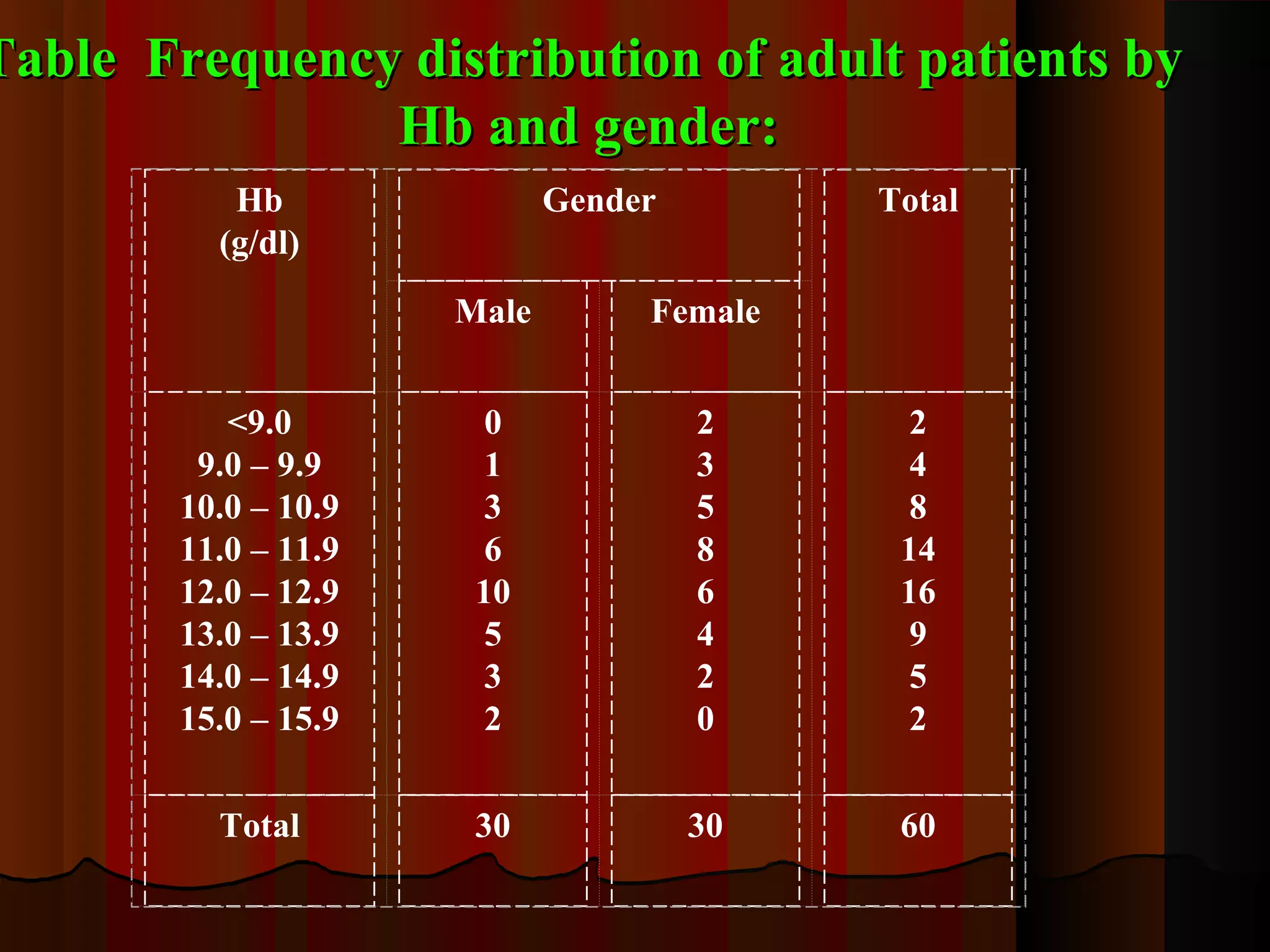
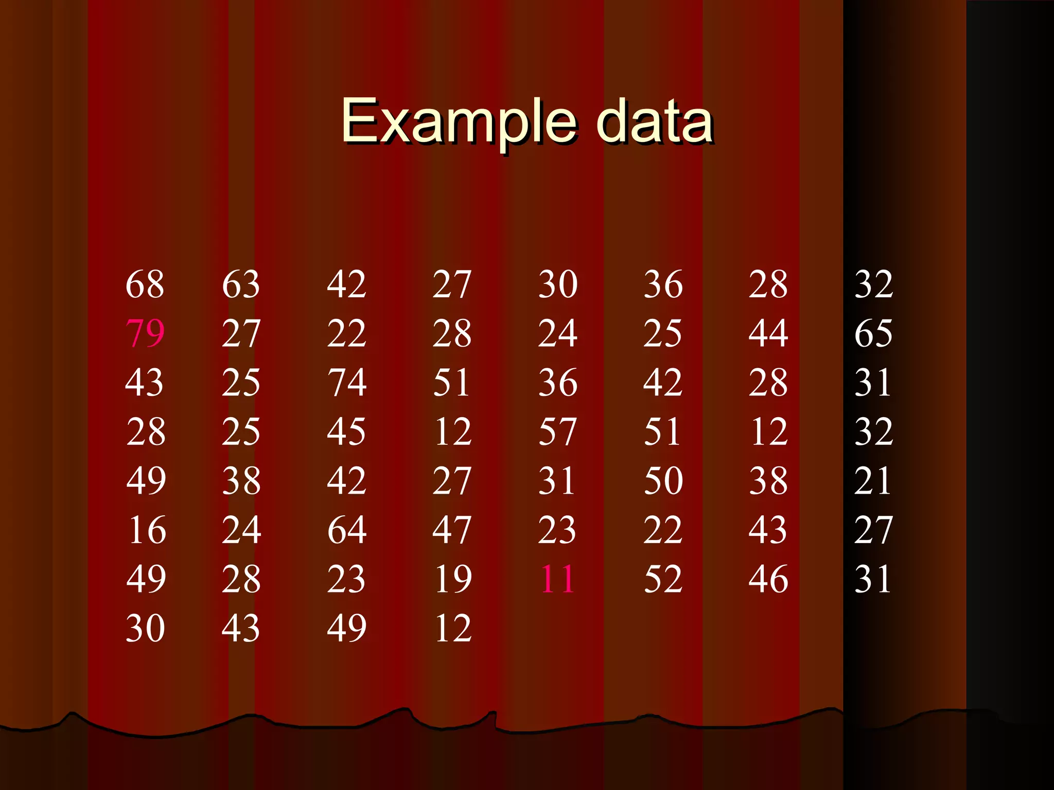
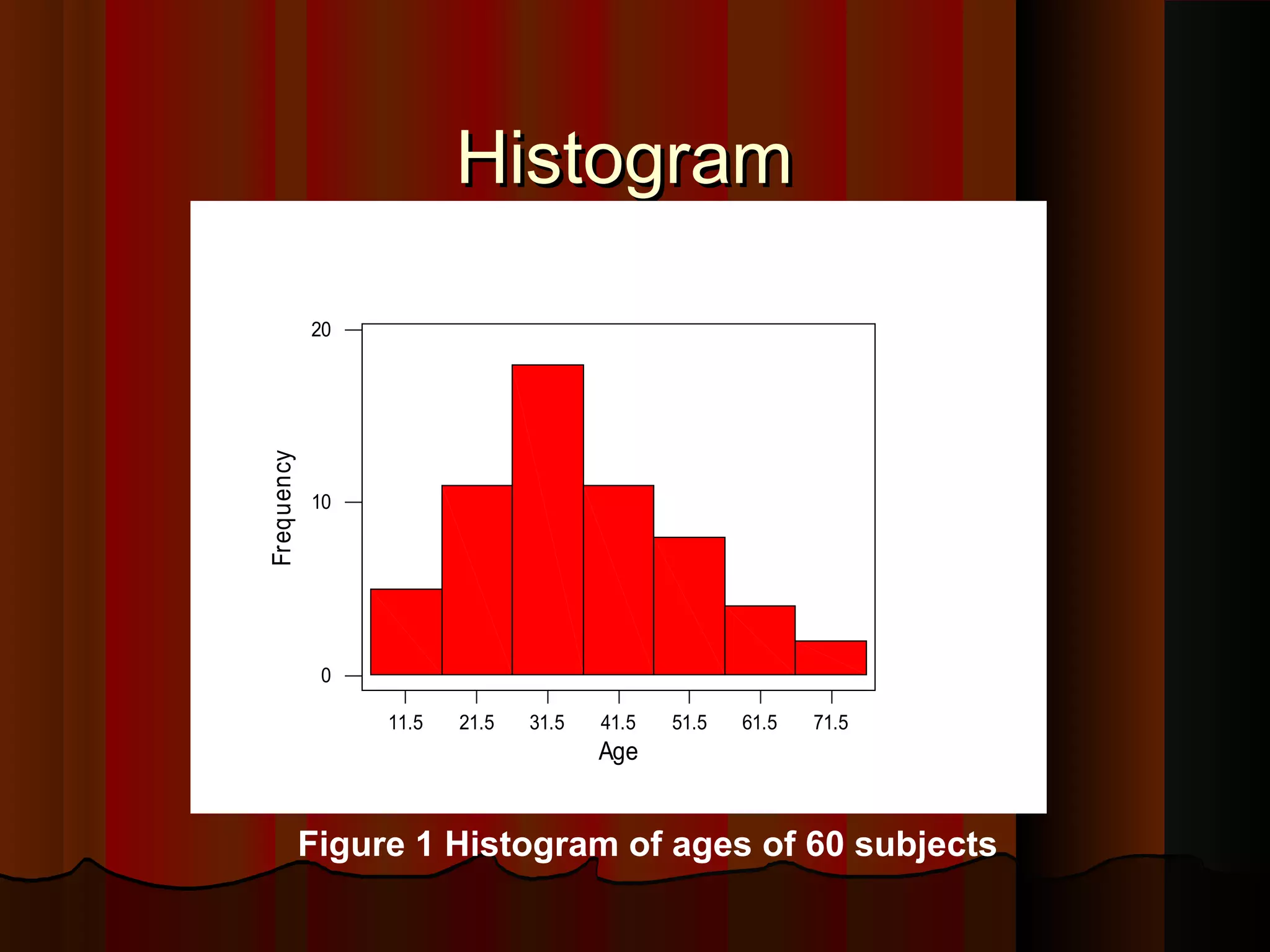
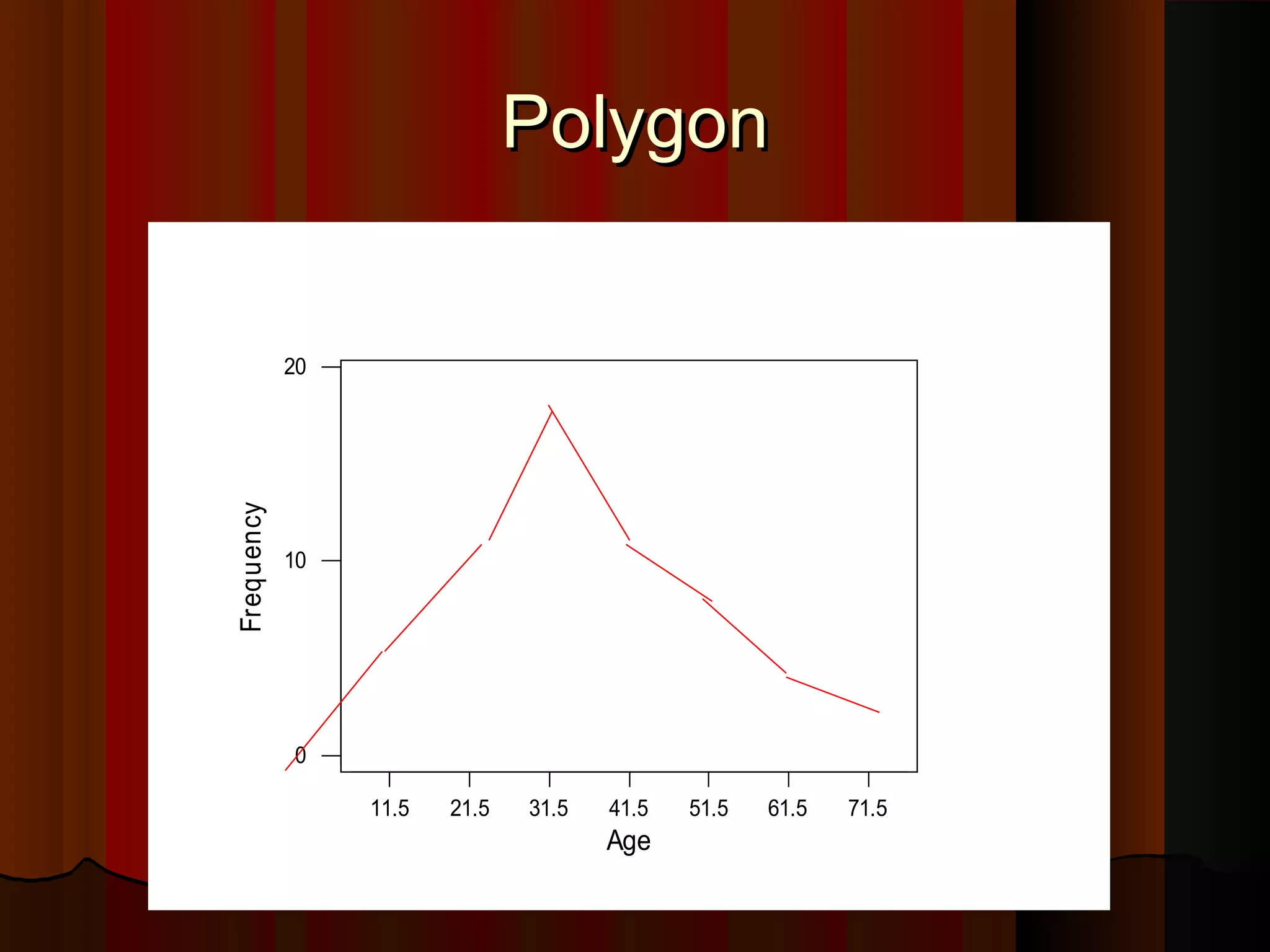
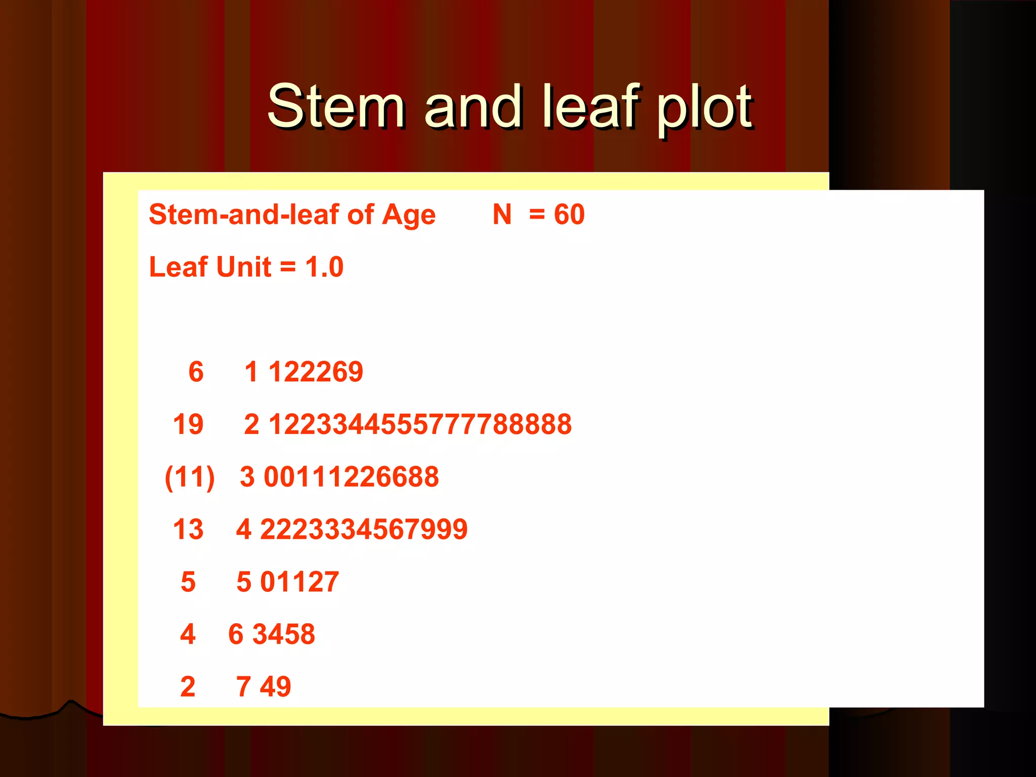
INTRODUCTION TOINTRODUCTION TO
BIOSTATISTICS IN NURSINGBIOSTATISTICS IN NURSING
Mr.MIDHUN KURIANMr.MIDHUN KURIAN
Associate . ProfessorAssociate . Professor
Dept. of Pediatric NursingDept. of Pediatric Nursing
SGRRCOLLEGE OF NURSINGSGRRCOLLEGE OF NURSING
SGRR UNIVERSITYSGRR UNIVERSITY
This session covers:This session covers:
 Introduction and development ofIntroduction and development of
BiostatisticsBiostatistics
 Definition of Statistics and BiostatisticsDefinition of Statistics and Biostatistics
 Reasons to know about BiostatisticsReasons to know about Biostatistics
 Types of dataTypes of data
 Graphical representation of a dataGraphical representation of a data
 Frequency distribution of a dataFrequency distribution of a data
““Statistics is the science whichStatistics is the science which
deals with collection,deals with collection,
classification and tabulation ofclassification and tabulation of
numerical facts as the basis fornumerical facts as the basis for
explanation, description andexplanation, description and
comparison of phenomenon”.comparison of phenomenon”.
------ Lovitt------ Lovitt
Origin and development of statistics inOrigin and development of statistics in
Medical ResearchMedical Research
In 1929 a huge paper on application ofIn 1929 a huge paper on application of
statistics was published in Physiologystatistics was published in Physiology
Journal by Dunn.Journal by Dunn.
In 1937, 15 articles on statistical methodsIn 1937, 15 articles on statistical methods
by Austin Bradford Hill, were published inby Austin Bradford Hill, were published in
book form.book form.
In 1948, a RCT of Streptomycin forIn 1948, a RCT of Streptomycin for
pulmonary tb., was published in whichpulmonary tb., was published in which
Bradford Hill has a key influence.Bradford Hill has a key influence.
Then the growth of Statistics in MedicineThen the growth of Statistics in Medicine
from 1952 was a 8-fold increase by 1982.from 1952 was a 8-fold increase by 1982.
Douglas Altman Ronald Fisher Karl Pearson
C.R. Rao
Gauss -
““BIOSTATISICSBIOSTATISICS””
(1) Statistics arising out of biological(1) Statistics arising out of biological
sciences, particularly from the fields ofsciences, particularly from the fields of
Medicine and public health.Medicine and public health.
(2) The methods used in dealing with(2) The methods used in dealing with
statistics in the fields of medicine, biologystatistics in the fields of medicine, biology
and public health for planning, conductingand public health for planning, conducting
and analyzing data which arise inand analyzing data which arise in
investigations of these branches.investigations of these branches.
Reasons to know about biostatistics:Reasons to know about biostatistics:
Medicine is becoming increasinglyMedicine is becoming increasingly
quantitative.quantitative.
The planning, conduct and interpretationThe planning, conduct and interpretation
of much of medical research are becomingof much of medical research are becoming
increasingly reliant on the statisticalincreasingly reliant on the statistical
methodology.methodology.
Statistics pervades the medical literature.Statistics pervades the medical literature.
WHAT DOES STAISTICSWHAT DOES STAISTICS
COVER ?COVER ?
PlanningPlanning
DesignDesign
Execution (Data collection)Execution (Data collection)
Data ProcessingData Processing
Data analysisData analysis
PresentationPresentation
InterpretationInterpretation
PublicationPublication
HOW A “BIOSTATISTICIAN” CANHOW A “BIOSTATISTICIAN” CAN
HELP ?HELP ?
Design of studyDesign of study
Sample size & power calculationsSample size & power calculations
Selection of sample and controlsSelection of sample and controls
Designing a questionnaireDesigning a questionnaire
Data ManagementData Management
Choice of descriptive statistics & graphsChoice of descriptive statistics & graphs
Application of univariate and multivariateApplication of univariate and multivariate
statistical analysis techniquesstatistical analysis techniques
TYPES OF DATATYPES OF DATA
QUALITATIVE DATAQUALITATIVE DATA
DISCRETE QUANTITATIVEDISCRETE QUANTITATIVE
CONTINOUS QUANTITATIVECONTINOUS QUANTITATIVE
QUALITATIVEQUALITATIVE
NominalNominal
Example: Sex ( M, F)Example: Sex ( M, F)
Exam result (P, F)Exam result (P, F)
Blood Group (A,B, O or AB)Blood Group (A,B, O or AB)
Color of Eyes (blue, green,Color of Eyes (blue, green,
brown, black)brown, black)
ORDINALORDINAL
Example:Example:
Response to treatmentResponse to treatment
(poor, fair, good)(poor, fair, good)
Severity of diseaseSeverity of disease
(mild, moderate, severe)(mild, moderate, severe)
Income status (low, middle,Income status (low, middle,
high)high)
QUANTITATIVE (DISCRETE)QUANTITATIVE (DISCRETE)
Example: The no. of family membersExample: The no. of family members
The no. of heart beatsThe no. of heart beats
The no. of admissions in a dayThe no. of admissions in a day
QUANTITATIVE (CONTINOUS)QUANTITATIVE (CONTINOUS)
Example: Height, Weight, Age, BP,Example: Height, Weight, Age, BP,
SerumSerum
Cholesterol and BMICholesterol and BMI
Discrete data -- Gaps between possible values
Continuous data -- Theoretically,
no gaps between possible values
Number of Children
Hb
CONTINUOUS DATACONTINUOUS DATA
DISCRETE DATADISCRETE DATA
wt. (in Kg.) : under wt, normal & over wt.wt. (in Kg.) : under wt, normal & over wt.
Ht. (in cm.): short, medium & tallHt. (in cm.): short, medium & tall
hospital length of stay Number Percent
1 – 3 days 5891 43.3
4 – 7 days 3489 25.6
2 weeks 2449 18.0
3 weeks 813 6.0
1 month 417 3.1
More than 1 month 545 4.0
Total 14604 100.0
Mean = 7.85 SE = 0.10
Table 1 Distribution of blunt injured patients
according to hospital length of stay
Scale of measurementScale of measurement
Qualitative variable:
A categorical variable
Nominal (classificatory) scale
- gender, marital status, race
Ordinal (ranking) scale
- severity scale, good/better/best
Scale of measurementScale of measurement
Quantitative variable:
A numerical variable: discrete; continuous
Interval scale :
Data is placed in meaningful intervals and order. The unit of
measurement are arbitrary.
- Temperature (37º C -- 36º C; 38º C-- 37º C are equal) and
No implication of ratio (30º C is not twice as hot as 15º C)
Ratio scale:
Data is presented in frequency distribution in
logical order. A meaningful ratio exists.
- Age, weight, height, pulse rate
- pulse rate of 120 is twice as fast as 60
- person with weight of 80kg is twice as heavy
as the one with weight of 40 kg.
Scales of MeasureScales of Measure
 NominalNominal – qualitative classification of– qualitative classification of
equal value: gender, race, color, cityequal value: gender, race, color, city
 OrdinalOrdinal - qualitative classification- qualitative classification
which can be rank ordered:which can be rank ordered:
socioeconomic status of familiessocioeconomic status of families
 IntervalInterval - Numerical or quantitative- Numerical or quantitative
data: can be rank ordered and sizesdata: can be rank ordered and sizes
compared : temperaturecompared : temperature
 RatioRatio - Quantitative interval data along- Quantitative interval data along
with ratio: time, age.with ratio: time, age.
INVESTIGATIONINVESTIGATION
Data Colllection
Data Presentation
Tabulation
Diagrams
Graphs
Descriptive Statistics
Measures of Location
Measures of Dispersion
Measures of Skewness &
Kurtosis
Inferential Statistiscs
Estimation Hypothesis
Testing
Ponit estimate
Inteval estimate
Univariate analysis
Multivariate analysis
Frequency DistributionsFrequency Distributions
data distribution – pattern ofdata distribution – pattern of
variability.variability.
the center of a distributionthe center of a distribution
the rangesthe ranges
the shapesthe shapes
simple frequency distributionssimple frequency distributions
grouped frequency distributionsgrouped frequency distributions
midpointmidpoint
PatienPatien
t Not No
HbHb
(g/dl)(g/dl)
PatienPatien
t Not No
HbHb
(g/dl)(g/dl)
PatienPatien
t Not No
HbHb
(g/dl)(g/dl)
11 12.012.0 1111 11.211.2 2121 14.914.9
22 11.911.9 1212 13.613.6 2222 12.212.2
33 11.511.5 1313 10.810.8 2323 12.212.2
44 14.214.2 1414 12.312.3 2424 11.411.4
55 12.312.3 1515 12.312.3 2525 10.710.7
66 13.013.0 1616 15.715.7 2626 12.512.5
77 10.510.5 1717 12.612.6 2727 11.811.8
88 12.812.8 1818 9.19.1 2828 15.115.1
99 13.213.2 1919 12.912.9 2929 13.413.4
1010 11.211.2 2020 14.614.6 3030 13.113.1
Tabulate the hemoglobin values of 30 adultTabulate the hemoglobin values of 30 adult
male patients listed belowmale patients listed below
Steps for making a tableSteps for making a table
Step1 Find Minimum (9.1) & MaximumStep1 Find Minimum (9.1) & Maximum
(15.7)(15.7)
Step2 Calculate difference 15.7 – 9.1 = 6.6Step2 Calculate difference 15.7 – 9.1 = 6.6
Step3 Decide the number and width ofStep3 Decide the number and width of
the classes (7 c.l) 9.0 -9.9, 10.0-the classes (7 c.l) 9.0 -9.9, 10.0-
10.9,----10.9,----
Step4 Prepare dummy table –Step4 Prepare dummy table –
Hb (g/dl), Tally mark, No. patientsHb (g/dl), Tally mark, No. patients
Hb (g/dl) Tall marks No.
patients
9.0 – 9.9
10.0 – 10.9
11.0 – 11.9
12.0 – 12.9
13.0 – 13.9
14.0 – 14.9
15.0 – 15.9
Total
Hb (g/dl) Tall marks No.
patients
9.0 – 9.9
10.0 – 10.9
11.0 – 11.9
12.0 – 12.9
13.0 – 13.9
14.0 – 14.9
15.0 – 15.9
l
lll
lll
llll llll
llll
lll
ll
1
3
6
10
5
3
2
Total - 30
DUMMY TABLEDUMMY TABLE Tall Marks TABLETall Marks TABLE
Hb (g/dl) No. of
patients
9.0 – 9.9
10.0 – 10.9
11.0 – 11.9
12.0 – 12.9
13.0 – 13.9
14.0 – 14.9
15.0 – 15.9
1
3
6
10
5
3
2
Total 30
Table Frequency distribution of 30 adult maleTable Frequency distribution of 30 adult male
patients by Hbpatients by Hb
Table Frequency distribution of adult patients byTable Frequency distribution of adult patients by
Hb and gender:Hb and gender:
Hb
(g/dl)
Gender Total
Male Female
<9.0
9.0 – 9.9
10.0 – 10.9
11.0 – 11.9
12.0 – 12.9
13.0 – 13.9
14.0 – 14.9
15.0 – 15.9
0
1
3
6
10
5
3
2
2
3
5
8
6
4
2
0
2
4
8
14
16
9
5
2
Total 30 30 60
Elements of a TableElements of a Table
Ideal table should have Number
Title
Column headings
Foot-notes
Number – Table number for identification in a report
Title,place - Describe the body of the table, variables,
Time period (What, how classified, where and when)
Column - Variable name, No. , Percentages (%), etc.,
Heading
Foot-note(s) - to describe some column/row headings,
special cells, source, etc.,
Death rate (/1000 per annum)No. of divisions
7.0-7.9 4 (3.3)
8.0 - 8.9 13 (10.8)
9.0 - 9.9 20 (16.7)
10.0 - 10.9 27 (22.5)
11.0 - 11.9 18 (15.0)
12.0 - 12.9 11 (0.2)
13.0 - 13.9 11 (9.2)
14.0 - 14.9 6 (5.0)
15.0 - 15.9 2 (1.7)
16.0 - 16.9 4 (3.3)
17.0 - 18.9 3 (2.5)
19.0 + 1 (0.8)
Total 120 (100.0)
Table II. Distribution of 120 (Madras) Corporation divisions
according to annual death rate based on registered deaths in
1975 and 1976
Figures in parentheses indicate percentages
DIAGRAMS/GRAPHSDIAGRAMS/GRAPHS
Discrete dataDiscrete data
--- Bar charts (one or two groups)--- Bar charts (one or two groups)
Continuous dataContinuous data
--- Histogram--- Histogram
--- Frequency polygon (curve)--- Frequency polygon (curve)
--- Stem-and –leaf plot--- Stem-and –leaf plot
--- Box-and-whisker plot--- Box-and-whisker plot
Example dataExample data
68 63 42 27 30 36 28 32
79 27 22 28 24 25 44 65
43 25 74 51 36 42 28 31
28 25 45 12 57 51 12 32
49 38 42 27 31 50 38 21
16 24 64 47 23 22 43 27
49 28 23 19 11 52 46 31
30 43 49 12
HistogramHistogram
Figure 1 Histogram of ages of 60 subjects
11.5 21.5 31.5 41.5 51.5 61.5 71.5
0
10
20
Age
Frequency
PolygonPolygon
71.561.551.541.531.521.511.5
20
10
0
Age
Frequency
Example dataExample data
68 63 42 27 30 36 28 32
79 27 22 28 24 25 44 65
43 25 74 51 36 42 28 31
28 25 45 12 57 51 12 32
49 38 42 27 31 50 38 21
16 24 64 47 23 22 43 27
49 28 23 19 11 52 46 31
30 43 49 12
Stem and leaf plotStem and leaf plot
Stem-and-leaf of Age N = 60
Leaf Unit = 1.0
6 1 122269
19 2 1223344555777788888
(11) 3 00111226688
13 4 2223334567999
5 5 01127
4 6 3458
2 7 49
Box plotBox plot
10
20
30
40
50
60
70
80
Age
Descriptive statistics report: BoxplotDescriptive statistics report: Boxplot
- minimum score
- maximum score
- lower quartile
- upper quartile
- median
- mean
- the skew of the distribution:
positive skew: mean > median & high-score whisker is longer
negative skew: mean < median & low-score whisker is longer
10%
20%
70%
Mild
Moderate
Severe
The prevalence of different degree of
Hypertension
in the population
Pie Chart
•Circular diagram – total -100%
•Divided into segments each
representing a category
•Decide adjacent category
•The amount for each category is
proportional to slice of the pie
Bar GraphsBar Graphs
9
12
20
16
12
8
20
0
5
10
15
20
25
Smo Alc Chol DM HTN No
Exer
F-H
Riskfactor
Number
The distribution of risk factor among cases with
Cardio vascular Diseases
Heights of the bar indicates
frequency
Frequency in the Y axis
and categories of variable
in the X axis
The bars should be of equal
width and no touching the
other bars
HIV cases enrolment in USA byHIV cases enrolment in USA by
gendergender
0
2
4
6
8
10
12
1986 1987 1988 1989 1990 1991 1992
Year
Enrollment(hundred)
Men
Women
Bar chart
HIV cases EnrollmentHIV cases Enrollment
in USA by genderin USA by gender
0
2
4
6
8
10
12
14
16
18
1986 1987 1988 1989 1990 1991 1992
Year
Enrollment(Thousands)
Women
Men
Stocked bar chart
Graphic Presentation of DataGraphic Presentation of Data
the histogram
(quantitative data)
the bar graph
(qualitative data)
the frequency polygon
(quantitative data)
General rules for designing graphsGeneral rules for designing graphs
 A graph should have a self-explanatoryA graph should have a self-explanatory
legendlegend
 A graph should help reader toA graph should help reader to
understand dataunderstand data
 Axis labeled, units of measurementAxis labeled, units of measurement
indicatedindicated
 Scales important. Start with zeroScales important. Start with zero
(otherwise // break)(otherwise // break)
 Avoid graphs with three-dimensionalAvoid graphs with three-dimensional
impression, it may be misleading (readerimpression, it may be misleading (reader
visualize less easilyvisualize less easily
Any QuestionsAny Questions

Biostatics introduction

  • 1.
    INTRODUCTION TOINTRODUCTION TO BIOSTATISTICSIN NURSINGBIOSTATISTICS IN NURSING Mr.MIDHUN KURIANMr.MIDHUN KURIAN Associate . ProfessorAssociate . Professor Dept. of Pediatric NursingDept. of Pediatric Nursing SGRRCOLLEGE OF NURSINGSGRRCOLLEGE OF NURSING SGRR UNIVERSITYSGRR UNIVERSITY
  • 2.
    This session covers:Thissession covers:  Introduction and development ofIntroduction and development of BiostatisticsBiostatistics  Definition of Statistics and BiostatisticsDefinition of Statistics and Biostatistics  Reasons to know about BiostatisticsReasons to know about Biostatistics  Types of dataTypes of data  Graphical representation of a dataGraphical representation of a data  Frequency distribution of a dataFrequency distribution of a data
  • 3.
    ““Statistics is thescience whichStatistics is the science which deals with collection,deals with collection, classification and tabulation ofclassification and tabulation of numerical facts as the basis fornumerical facts as the basis for explanation, description andexplanation, description and comparison of phenomenon”.comparison of phenomenon”. ------ Lovitt------ Lovitt
  • 4.
    Origin and developmentof statistics inOrigin and development of statistics in Medical ResearchMedical Research In 1929 a huge paper on application ofIn 1929 a huge paper on application of statistics was published in Physiologystatistics was published in Physiology Journal by Dunn.Journal by Dunn. In 1937, 15 articles on statistical methodsIn 1937, 15 articles on statistical methods by Austin Bradford Hill, were published inby Austin Bradford Hill, were published in book form.book form. In 1948, a RCT of Streptomycin forIn 1948, a RCT of Streptomycin for pulmonary tb., was published in whichpulmonary tb., was published in which Bradford Hill has a key influence.Bradford Hill has a key influence. Then the growth of Statistics in MedicineThen the growth of Statistics in Medicine from 1952 was a 8-fold increase by 1982.from 1952 was a 8-fold increase by 1982.
  • 5.
    Douglas Altman RonaldFisher Karl Pearson C.R. Rao Gauss -
  • 6.
    ““BIOSTATISICSBIOSTATISICS”” (1) Statistics arisingout of biological(1) Statistics arising out of biological sciences, particularly from the fields ofsciences, particularly from the fields of Medicine and public health.Medicine and public health. (2) The methods used in dealing with(2) The methods used in dealing with statistics in the fields of medicine, biologystatistics in the fields of medicine, biology and public health for planning, conductingand public health for planning, conducting and analyzing data which arise inand analyzing data which arise in investigations of these branches.investigations of these branches.
  • 7.
    Reasons to knowabout biostatistics:Reasons to know about biostatistics: Medicine is becoming increasinglyMedicine is becoming increasingly quantitative.quantitative. The planning, conduct and interpretationThe planning, conduct and interpretation of much of medical research are becomingof much of medical research are becoming increasingly reliant on the statisticalincreasingly reliant on the statistical methodology.methodology. Statistics pervades the medical literature.Statistics pervades the medical literature.
  • 8.
    WHAT DOES STAISTICSWHATDOES STAISTICS COVER ?COVER ? PlanningPlanning DesignDesign Execution (Data collection)Execution (Data collection) Data ProcessingData Processing Data analysisData analysis PresentationPresentation InterpretationInterpretation PublicationPublication
  • 9.
    HOW A “BIOSTATISTICIAN”CANHOW A “BIOSTATISTICIAN” CAN HELP ?HELP ? Design of studyDesign of study Sample size & power calculationsSample size & power calculations Selection of sample and controlsSelection of sample and controls Designing a questionnaireDesigning a questionnaire Data ManagementData Management Choice of descriptive statistics & graphsChoice of descriptive statistics & graphs Application of univariate and multivariateApplication of univariate and multivariate statistical analysis techniquesstatistical analysis techniques
  • 10.
    TYPES OF DATATYPESOF DATA QUALITATIVE DATAQUALITATIVE DATA DISCRETE QUANTITATIVEDISCRETE QUANTITATIVE CONTINOUS QUANTITATIVECONTINOUS QUANTITATIVE
  • 11.
    QUALITATIVEQUALITATIVE NominalNominal Example: Sex (M, F)Example: Sex ( M, F) Exam result (P, F)Exam result (P, F) Blood Group (A,B, O or AB)Blood Group (A,B, O or AB) Color of Eyes (blue, green,Color of Eyes (blue, green, brown, black)brown, black)
  • 12.
    ORDINALORDINAL Example:Example: Response to treatmentResponseto treatment (poor, fair, good)(poor, fair, good) Severity of diseaseSeverity of disease (mild, moderate, severe)(mild, moderate, severe) Income status (low, middle,Income status (low, middle, high)high)
  • 13.
    QUANTITATIVE (DISCRETE)QUANTITATIVE (DISCRETE) Example:The no. of family membersExample: The no. of family members The no. of heart beatsThe no. of heart beats The no. of admissions in a dayThe no. of admissions in a day QUANTITATIVE (CONTINOUS)QUANTITATIVE (CONTINOUS) Example: Height, Weight, Age, BP,Example: Height, Weight, Age, BP, SerumSerum Cholesterol and BMICholesterol and BMI
  • 14.
    Discrete data --Gaps between possible values Continuous data -- Theoretically, no gaps between possible values Number of Children Hb
  • 15.
    CONTINUOUS DATACONTINUOUS DATA DISCRETEDATADISCRETE DATA wt. (in Kg.) : under wt, normal & over wt.wt. (in Kg.) : under wt, normal & over wt. Ht. (in cm.): short, medium & tallHt. (in cm.): short, medium & tall
  • 16.
    hospital length ofstay Number Percent 1 – 3 days 5891 43.3 4 – 7 days 3489 25.6 2 weeks 2449 18.0 3 weeks 813 6.0 1 month 417 3.1 More than 1 month 545 4.0 Total 14604 100.0 Mean = 7.85 SE = 0.10 Table 1 Distribution of blunt injured patients according to hospital length of stay
  • 17.
    Scale of measurementScaleof measurement Qualitative variable: A categorical variable Nominal (classificatory) scale - gender, marital status, race Ordinal (ranking) scale - severity scale, good/better/best
  • 18.
    Scale of measurementScaleof measurement Quantitative variable: A numerical variable: discrete; continuous Interval scale : Data is placed in meaningful intervals and order. The unit of measurement are arbitrary. - Temperature (37º C -- 36º C; 38º C-- 37º C are equal) and No implication of ratio (30º C is not twice as hot as 15º C)
  • 19.
    Ratio scale: Data ispresented in frequency distribution in logical order. A meaningful ratio exists. - Age, weight, height, pulse rate - pulse rate of 120 is twice as fast as 60 - person with weight of 80kg is twice as heavy as the one with weight of 40 kg.
  • 20.
    Scales of MeasureScalesof Measure  NominalNominal – qualitative classification of– qualitative classification of equal value: gender, race, color, cityequal value: gender, race, color, city  OrdinalOrdinal - qualitative classification- qualitative classification which can be rank ordered:which can be rank ordered: socioeconomic status of familiessocioeconomic status of families  IntervalInterval - Numerical or quantitative- Numerical or quantitative data: can be rank ordered and sizesdata: can be rank ordered and sizes compared : temperaturecompared : temperature  RatioRatio - Quantitative interval data along- Quantitative interval data along with ratio: time, age.with ratio: time, age.
  • 24.
    INVESTIGATIONINVESTIGATION Data Colllection Data Presentation Tabulation Diagrams Graphs DescriptiveStatistics Measures of Location Measures of Dispersion Measures of Skewness & Kurtosis Inferential Statistiscs Estimation Hypothesis Testing Ponit estimate Inteval estimate Univariate analysis Multivariate analysis
  • 25.
    Frequency DistributionsFrequency Distributions datadistribution – pattern ofdata distribution – pattern of variability.variability. the center of a distributionthe center of a distribution the rangesthe ranges the shapesthe shapes simple frequency distributionssimple frequency distributions grouped frequency distributionsgrouped frequency distributions midpointmidpoint
  • 26.
    PatienPatien t Not No HbHb (g/dl)(g/dl) PatienPatien tNot No HbHb (g/dl)(g/dl) PatienPatien t Not No HbHb (g/dl)(g/dl) 11 12.012.0 1111 11.211.2 2121 14.914.9 22 11.911.9 1212 13.613.6 2222 12.212.2 33 11.511.5 1313 10.810.8 2323 12.212.2 44 14.214.2 1414 12.312.3 2424 11.411.4 55 12.312.3 1515 12.312.3 2525 10.710.7 66 13.013.0 1616 15.715.7 2626 12.512.5 77 10.510.5 1717 12.612.6 2727 11.811.8 88 12.812.8 1818 9.19.1 2828 15.115.1 99 13.213.2 1919 12.912.9 2929 13.413.4 1010 11.211.2 2020 14.614.6 3030 13.113.1 Tabulate the hemoglobin values of 30 adultTabulate the hemoglobin values of 30 adult male patients listed belowmale patients listed below
  • 27.
    Steps for makinga tableSteps for making a table Step1 Find Minimum (9.1) & MaximumStep1 Find Minimum (9.1) & Maximum (15.7)(15.7) Step2 Calculate difference 15.7 – 9.1 = 6.6Step2 Calculate difference 15.7 – 9.1 = 6.6 Step3 Decide the number and width ofStep3 Decide the number and width of the classes (7 c.l) 9.0 -9.9, 10.0-the classes (7 c.l) 9.0 -9.9, 10.0- 10.9,----10.9,---- Step4 Prepare dummy table –Step4 Prepare dummy table – Hb (g/dl), Tally mark, No. patientsHb (g/dl), Tally mark, No. patients
  • 28.
    Hb (g/dl) Tallmarks No. patients 9.0 – 9.9 10.0 – 10.9 11.0 – 11.9 12.0 – 12.9 13.0 – 13.9 14.0 – 14.9 15.0 – 15.9 Total Hb (g/dl) Tall marks No. patients 9.0 – 9.9 10.0 – 10.9 11.0 – 11.9 12.0 – 12.9 13.0 – 13.9 14.0 – 14.9 15.0 – 15.9 l lll lll llll llll llll lll ll 1 3 6 10 5 3 2 Total - 30 DUMMY TABLEDUMMY TABLE Tall Marks TABLETall Marks TABLE
  • 29.
    Hb (g/dl) No.of patients 9.0 – 9.9 10.0 – 10.9 11.0 – 11.9 12.0 – 12.9 13.0 – 13.9 14.0 – 14.9 15.0 – 15.9 1 3 6 10 5 3 2 Total 30 Table Frequency distribution of 30 adult maleTable Frequency distribution of 30 adult male patients by Hbpatients by Hb
  • 30.
    Table Frequency distributionof adult patients byTable Frequency distribution of adult patients by Hb and gender:Hb and gender: Hb (g/dl) Gender Total Male Female <9.0 9.0 – 9.9 10.0 – 10.9 11.0 – 11.9 12.0 – 12.9 13.0 – 13.9 14.0 – 14.9 15.0 – 15.9 0 1 3 6 10 5 3 2 2 3 5 8 6 4 2 0 2 4 8 14 16 9 5 2 Total 30 30 60
  • 31.
    Elements of aTableElements of a Table Ideal table should have Number Title Column headings Foot-notes Number – Table number for identification in a report Title,place - Describe the body of the table, variables, Time period (What, how classified, where and when) Column - Variable name, No. , Percentages (%), etc., Heading Foot-note(s) - to describe some column/row headings, special cells, source, etc.,
  • 32.
    Death rate (/1000per annum)No. of divisions 7.0-7.9 4 (3.3) 8.0 - 8.9 13 (10.8) 9.0 - 9.9 20 (16.7) 10.0 - 10.9 27 (22.5) 11.0 - 11.9 18 (15.0) 12.0 - 12.9 11 (0.2) 13.0 - 13.9 11 (9.2) 14.0 - 14.9 6 (5.0) 15.0 - 15.9 2 (1.7) 16.0 - 16.9 4 (3.3) 17.0 - 18.9 3 (2.5) 19.0 + 1 (0.8) Total 120 (100.0) Table II. Distribution of 120 (Madras) Corporation divisions according to annual death rate based on registered deaths in 1975 and 1976 Figures in parentheses indicate percentages
  • 33.
    DIAGRAMS/GRAPHSDIAGRAMS/GRAPHS Discrete dataDiscrete data ---Bar charts (one or two groups)--- Bar charts (one or two groups) Continuous dataContinuous data --- Histogram--- Histogram --- Frequency polygon (curve)--- Frequency polygon (curve) --- Stem-and –leaf plot--- Stem-and –leaf plot --- Box-and-whisker plot--- Box-and-whisker plot
  • 34.
    Example dataExample data 6863 42 27 30 36 28 32 79 27 22 28 24 25 44 65 43 25 74 51 36 42 28 31 28 25 45 12 57 51 12 32 49 38 42 27 31 50 38 21 16 24 64 47 23 22 43 27 49 28 23 19 11 52 46 31 30 43 49 12
  • 35.
    HistogramHistogram Figure 1 Histogramof ages of 60 subjects 11.5 21.5 31.5 41.5 51.5 61.5 71.5 0 10 20 Age Frequency
  • 36.
  • 37.
    Example dataExample data 6863 42 27 30 36 28 32 79 27 22 28 24 25 44 65 43 25 74 51 36 42 28 31 28 25 45 12 57 51 12 32 49 38 42 27 31 50 38 21 16 24 64 47 23 22 43 27 49 28 23 19 11 52 46 31 30 43 49 12
  • 38.
    Stem and leafplotStem and leaf plot Stem-and-leaf of Age N = 60 Leaf Unit = 1.0 6 1 122269 19 2 1223344555777788888 (11) 3 00111226688 13 4 2223334567999 5 5 01127 4 6 3458 2 7 49
  • 39.
  • 40.
    Descriptive statistics report:BoxplotDescriptive statistics report: Boxplot - minimum score - maximum score - lower quartile - upper quartile - median - mean - the skew of the distribution: positive skew: mean > median & high-score whisker is longer negative skew: mean < median & low-score whisker is longer
  • 41.
    10% 20% 70% Mild Moderate Severe The prevalence ofdifferent degree of Hypertension in the population Pie Chart •Circular diagram – total -100% •Divided into segments each representing a category •Decide adjacent category •The amount for each category is proportional to slice of the pie
  • 42.
    Bar GraphsBar Graphs 9 12 20 16 12 8 20 0 5 10 15 20 25 SmoAlc Chol DM HTN No Exer F-H Riskfactor Number The distribution of risk factor among cases with Cardio vascular Diseases Heights of the bar indicates frequency Frequency in the Y axis and categories of variable in the X axis The bars should be of equal width and no touching the other bars
  • 43.
    HIV cases enrolmentin USA byHIV cases enrolment in USA by gendergender 0 2 4 6 8 10 12 1986 1987 1988 1989 1990 1991 1992 Year Enrollment(hundred) Men Women Bar chart
  • 44.
    HIV cases EnrollmentHIVcases Enrollment in USA by genderin USA by gender 0 2 4 6 8 10 12 14 16 18 1986 1987 1988 1989 1990 1991 1992 Year Enrollment(Thousands) Women Men Stocked bar chart
  • 45.
    Graphic Presentation ofDataGraphic Presentation of Data the histogram (quantitative data) the bar graph (qualitative data) the frequency polygon (quantitative data)
  • 47.
    General rules fordesigning graphsGeneral rules for designing graphs  A graph should have a self-explanatoryA graph should have a self-explanatory legendlegend  A graph should help reader toA graph should help reader to understand dataunderstand data  Axis labeled, units of measurementAxis labeled, units of measurement indicatedindicated  Scales important. Start with zeroScales important. Start with zero (otherwise // break)(otherwise // break)  Avoid graphs with three-dimensionalAvoid graphs with three-dimensional impression, it may be misleading (readerimpression, it may be misleading (reader visualize less easilyvisualize less easily
  • 48.

Editor's Notes

  • #21 Nominal variables allow for only qualitative classification. That is, they can be measured only in terms of whether the individual items belong to some distinctively different categories, but we cannot quantify or even rank order those categories. For example, all we can say is that 2 individuals are different in terms of variable A (e.g., they are of different race), but we cannot say which one &amp;quot;has more&amp;quot; of the quality represented by the variable. Typical examples of nominal variables are gender, race, color, city, etc. Ordinal variables allow us to rank order the items we measure in terms of which has less and which has more of the quality represented by the variable, but still they do not allow us to say &amp;quot;how much more.&amp;quot; A typical example of an ordinal variable is the socioeconomic status of families. For example, we know that upper-middle is higher than middle but we cannot say that it is, for example, 18% higher. Also this very distinction between nominal, ordinal, and interval scales itself represents a good example of an ordinal variable. For example, we can say that nominal measurement provides less information than ordinal measurement, but we cannot say &amp;quot;how much less&amp;quot; or how this difference compares to the difference between ordinal and interval scales. Interval variables allow us not only to rank order the items that are measured, but also to quantify and compare the sizes of differences between them. For example, temperature, as measured in degrees Fahrenheit or Celsius, constitutes an interval scale. We can say that a temperature of 40 degrees is higher than a temperature of 30 degrees, and that an increase from 20 to 40 degrees is twice as much as an increase from 30 to 40 degrees. Ratio variables are very similar to interval variables; in addition to all the properties of interval variables, they feature an identifiable absolute zero point, thus they allow for statements such as x is two times more than y. Typical examples of ratio scales are measures of time or space. For example, as the Kelvin temperature scale is a ratio scale, not only can we say that a temperature of 200 degrees is higher than one of 100 degrees, we can correctly state that it is twice as high. Interval scales do not have the ratio property. Most statistical data analysis procedures do not distinguish between the interval and ratio properties of the measurement scales.
  • #44 This shows relative trends in admissions by gender.
  • #45 This emphasizes the constancy of the overall admissions and shows the trends subtly.