This document covers Python data handling techniques such as file input/output, using libraries like NumPy and Pandas for data manipulation, and methods for data reading and writing. It discusses the differences between NumPy and Pandas in terms of performance and coding ease, as well as how to handle errors while managing files. The document also includes examples of accessing various file formats and illustrates functions for creating and manipulating arrays with NumPy.

1. Darshan Institute of Engineering & Technology, Rajkot
arjun.bala@darshan.ac.in
9624822202
Computer Engineering Department
Prof. Arjun V. Bala
Python for Data Science (PDS) (3150713)
Unit-03
Capturing,
Preparing and
Working with data

2.  Looping
Outline
Basic File IO in Python
NumPy V/S Pandas (what to use?)
NumPy
Pandas
Accessing text, CSV, Excel files using pandas
Accessing SQL Database
Web Scrapping using BeautifulSoup

3. Prof. Arjun V. Bala
#3150713 (PDS)  Unit 03 – Capturing, Preparing and Working
3
Basic IO operations in Python
 Before we can read or write a file, we have to open it using Python's built-in
open() function.
 filename is a name of a file we want to open.
 accessmode is determines the mode in which file has to be opened (list of possible values
given below)
 If buffering is set to 0, no buffering will happen, if set to 1 line buffering will happen, if
grater than 1 then the number of buffer and if negative is given it will follow system default
buffering behaviour.
fileobject = open(filename [, accessmode][,
buffering])
syntax
M Description
r Read only (default)
rb
Read only in binary
format
r+ Read and Write both
rb+
Read and Write both in
binary format
M Description (create file if not
exist)
w Write only
wb
Write only in binary
format
w+ Read and Write both
wb
+
Read and Write both in
binary format
M Description
a
Opens file to append, if
file not exist will create it
for write
ab
Append in binary format,
if file not exist will create
it for write
a+
Append, if file not exist it
will create for read &
write both

4. Prof. Arjun V. Bala
#3150713 (PDS)  Unit 03 – Capturing, Preparing and Working
4
Example : Read file in Python
 read(size) will read specified bytes from the file, if we don’t specify size it will
return whole file.
 reallines() method will return list of lines from the file.
 We can use for loop to get each line separately,
f = open('college.txt')
data = f.read()
print(data)
1
2
3
readfile.py
Darshan Institute of Engineering and Technology -
Rajkot
At Hadala, Rajkot - Morbi Highway,
Gujarat-363650, INDIA
college.txt
f = open('college.txt')
lines = f.readlines()
print(lines)
1
2
3
readlines.py
['Darshan Institute of Engineering and Technology -
Rajkotn', 'At Hadala, Rajkot - Morbi Highway,n',
'Gujarat-363650, INDIA']
OUTPUT
f = open('college.txt')
lines = f.readlines()
for l in lines :
print(l)
1
2
3
4
readlinesfor.py
Darshan Institute of Engineering and Technology -
Rajkot
At Hadala, Rajkot - Morbi Highway,
Gujarat-363650, INDIA
OUTPUT

5. Prof. Arjun V. Bala
#3150713 (PDS)  Unit 03 – Capturing, Preparing and Working
5
How to write path?
 We can specify relative path in argument to open method, alternatively we can
also specify absolute path.
 To specify absolute path,
 In windows, f=open(‘D:foldersubfolderfilename.txt’)
 In mac & linux, f=open(‘/user/folder/subfolder/filename.txt’)
 We suppose to close the file once we are done using the file in the Python using
close() method.
f = open('college.txt')
data = f.read()
print(data)
f.close()
1
2
3
4
closefile.py

6. Prof. Arjun V. Bala
#3150713 (PDS)  Unit 03 – Capturing, Preparing and Working
6
Handling errors using “with” keyword
 It is possible that we may have typo in the filename or file we specified is
moved/deleted, in such cases there will be an error while running the file.
 To handle such situations we can use new syntax of opening the file using with
keyword.
 When we open file using with we need not to close the file.
with open('college.txt') as f :
data = f.read()
print(data)
1
2
3
fileusingwith.py

7. Prof. Arjun V. Bala
#3150713 (PDS)  Unit 03 – Capturing, Preparing and Working
7
Example : Write file in Python
 write() method will write the specified data to the file.
 If we open file with ‘w’ mode it will overwrite the data to the existing file or will
create new file if file does not exists.
 If we open file with ‘a’ mode it will append the data at the end of the existing file
or will create new file if file does not exists.
with open('college.txt','a') as f
:
f.write('Hello world')
1
2
readdemo.py

8. Prof. Arjun V. Bala
#3150713 (PDS)  Unit 03 – Capturing, Preparing and Working
8
Reading CSV files without any library functions
 A comma-separated values file is a delimited text file that uses a comma to
separate values.
 Each line of is a data record, Each record consists of many fields, separated by
commas.
 Example :
 We can use Microsoft Excel to access
CSV files.
 In the later sessions we will access CSV
files using different libraries, but we can
also access CSV files without any libraries.
(Not recommend)
studentname,enrollment,cpi
abcd,123456,8.5
bcde,456789,2.5
cdef,321654,7.6
Book1.csv
with open('Book1.csv') as f :
rows = f.readlines()
for r in rows :
cols = r.split(',')
print('Student Name = ', cols[0], end="
")
print('tEn. No. = ', cols[1], end=" ")
print('tCPI = t', cols[2])
1
2
3
4
5
6
7
readlines.py
with open('Book1.csv') as f :
rows = f.readlines()
isFirstLine = True
for r in rows :
if isFirstLine :
isFirstLine = False
continue
cols = r.split(',')
print('Student Name = ', cols[0], end="
")
print('tEn. No. = ', cols[1], end=" ")
print('tCPI = t', cols[2])
1
2
3
4
5
6
7
8
9
10
11
readlines.py

9. Prof. Arjun V. Bala
#3150713 (PDS)  Unit 03 – Capturing, Preparing and Working
9
NumPy v/s Pandas
 Developers built pandas on top of NumPy, as a result every task we perform
using pandas also goes through NumPy.
 To obtain the benefits of pandas, we need to pay a performance penalty that
some testers say is 100 times slower than NumPy for similar task.
 Nowadays computer hardware are powerful enough to take care for the
performance issue, but when speed of execution is essential NumPy is always
the best choice.
 We can use pandas to make writing code easier and faster, pandas will reduce
potential coding errors.
 Pandas provide rich time-series functionality, data alignment, NA-friendly
statistics, groupby, merge, etc.. methods, if we use NumPy we have to
implement all these methods manually.
 So,
 if we want performance we should use NumPy,
 if we want ease of coding we should use pandas.

10. Darshan Institute of Engineering & Technology, Rajkot
arjun.bala@darshan.ac.in
9624822202
Computer Engineering Department
Prof. Arjun V. Bala
Python for Data Science (PDS) (3150713)
Unit-03.01
Lets Learn
NumPy

11. Prof. Arjun V. Bala
#3150713 (PDS)  Unit 03 – Capturing, Preparing and Working
11
NumPy
 NumPy (Numeric Python) is a Python library to manipulate arrays.
 Almost all the libraries in python rely on NumPy as one of their main building
block.
 NumPy provides functions for domains like Algebra, Fourier transform etc..
 NumPy is incredibly fast as it has bindings to C libraries.
 Install :
 conda install numpy
 pip install numpy
OR

12. Prof. Arjun V. Bala
#3150713 (PDS)  Unit 03 – Capturing, Preparing and Working
12
NumPy Array
 The most important object defined in NumPy is an N-dimensional array type
called ndarray.
 It describes the collection of items of the same type, Items in the collection
can be accessed using a zero-based index.
 An instance of ndarray class can be constructed in many different ways, the
basic ndarray can be created as below.
import numpy as np
a= np.array(list | tuple | set | dict)
syntax
import numpy as np
a=
np.array(['darshan','Insitute','rajkot'])
print(type(a))
print(a)
1
2
3
4
numpyarray.py
<class 'numpy.ndarray'>
['darshan' 'Insitute' 'rajkot']
Output

13. Prof. Arjun V. Bala
#3150713 (PDS)  Unit 03 – Capturing, Preparing and Working
13
NumPy Array (Cont.)
 arange(start,end,step) function will create NumPy array starting from start till
end (not included) with specified steps.
 zeros(n) function will return NumPy array of given shape, filled with zeros.
 ones(n) function will return NumPy array of given shape, filled with ones.
import numpy as np
b = np.arange(0,10,1)
print(b)
1
2
3
numpyarange.p
y
[0 1 2 3 4 5 6 7 8 9]
Output
import numpy as np
c = np.zeros(3)
print(c)
c1 = np.zeros((3,3)) #have to give as
tuple
print(c1)
1
2
3
4
5
numpyzeros.py
[0. 0. 0.]
[[0. 0. 0.] [0. 0. 0.] [0. 0. 0.]]
Output

14. Prof. Arjun V. Bala
#3150713 (PDS)  Unit 03 – Capturing, Preparing and Working
14
NumPy Array (Cont.)
 eye(n) function will create 2-D NumPy array with ones on the diagonal and zeros
elsewhere.
 linspace(start,stop,num) function will return evenly spaced numbers over a
specified interval.
 Note: in arange function we have given start, stop & step, whereas in lispace
function we are giving start,stop & number of elements we want.
import numpy as np
b = np.eye(3)
print(b)
1
2
3
numpyeye.py
[[1. 0. 0.]
[0. 1. 0.]
[0. 0. 1.]]
Output
import numpy as np
c = np.linspace(0,1,11)
print(c)
1
2
3
numpylinspace.
py
[0. 0.1 0.2 0.3 0.4 0.5 0.6 0.7
0.8 0.9 1. ]
Output

15. Prof. Arjun V. Bala
#3150713 (PDS)  Unit 03 – Capturing, Preparing and Working
15
Array Shape in NumPy
 We can grab the shape of ndarray using its shape property.
 We can also reshape the array using reshape method of ndarray.
 Note: the number of elements and multiplication of rows and cols in new array
must be equal.
 Example : here we have old one-dimensional array of 10 elements and reshaped shape is
(5,2)
so, 5 * 2 = 10, which means it is a valid reshape
import numpy as np
b = np.zeros((3,3))
print(b.shape)
1
2
3
numpyarange.p
y
(3,3)
Output
import numpy as np
re1 = np.random.randint(1,100,10)
re2 = re1.reshape(5,2)
print(re2)
1
2
3
4
numpyarange.p
y
[[29 55]
[44 50]
[25 53]
[59 6]
[93 7]]
Output

16. Prof. Arjun V. Bala
#3150713 (PDS)  Unit 03 – Capturing, Preparing and Working
16
NumPy Random
 rand(p1,p2….,pn) function will create n-dimensional array with random data
using uniform distrubution, if we do not specify any parameter it will return
random float number.
 randint(low,high,num) function will create one-dimensional array with num
random integer data between low and high.
 We can reshape the array in any shape using reshape method, which we
learned in previous slide.
import numpy as np
r1 = np.random.rand()
print(r1)
r2 = np.random.rand(3,2) # no
tuple
print(r2)
1
2
3
4
5
numpyrand.py
0.23937253208490505
[[0.58924723 0.09677878]
[0.97945337 0.76537675]
[0.73097381 0.51277276]]
Output
import numpy as np
r3 = np.random.randint(1,100,10)
print(r3)
1
2
3
numpyrandint.p
y
[78 78 17 98 19 26 81 67 23 24]
Output

17. Prof. Arjun V. Bala
#3150713 (PDS)  Unit 03 – Capturing, Preparing and Working
17
NumPy Random (Cont.)
 randn(p1,p2….,pn) function will create n-dimensional array with random data
using standard normal distribution, if we do not specify any parameter it will
return random float number.
 Note: rand function will generate random number using uniform distribution,
whereas randn function will generate random number using standard normal
distribution.
 We are going to learn the difference using visualization technique (as a data
scientist, We have to use visualization techniques to convince the audience)
import numpy as np
r1 = np.random.randn()
print(r1)
r2 = np.random.randn(3,2) # no
tuple
print(r2)
1
2
3
4
5
numpyrandn.py
-0.15359861758111037
[[ 0.40967905 -0.21974532]
[-0.90341482 -0.69779498]
[ 0.99444948 -1.45308348]]
Output

18. Prof. Arjun V. Bala
#3150713 (PDS)  Unit 03 – Capturing, Preparing and Working
18
Visualizing the difference between rand & randn
 We are going to use matplotlib library to visualize the difference.
 You need not to worry if you are not getting the syntax of matplotlib, we are going to learn
it in detail in Unit-4
import numpy as np
from matplotlib import pyplot as
plt
%matplotlib inline
samplesize = 100000
uniform =
np.random.rand(samplesize)
normal =
np.random.randn(samplesize)
plt.hist(uniform,bins=100)
plt.title('rand: uniform')
plt.show()
plt.hist(normal,bins=100)
plt.title('randn: normal')
plt.show()
1
2
3
4
5
6
7
8
9
10
11
12
matplotdemo.p
y

19. Prof. Arjun V. Bala
#3150713 (PDS)  Unit 03 – Capturing, Preparing and Working
19
Aggregations
 min() function will return the minimum value from the ndarray, there are two
ways in which we can use min function, example of both ways are given below.
 max() function will return the maximum value from the ndarray, there are two
ways in which we can use min function, example of both ways are given below.
import numpy as np
l =
[1,5,3,8,2,3,6,7,5,2,9,11,2,5,3,4,8,9,3,1,9,3]
a = np.array(l)
print('Min way1 = ',a.min())
print('Min way2 = ',np.min(a))
1
2
3
4
5
numpymin.py
Min way1 = 1
Min way2 = 1
Output
import numpy as np
l =
[1,5,3,8,2,3,6,7,5,2,9,11,2,5,3,4,8,9,3,1,9,3]
a = np.array(l)
print('Max way1 = ',a.max())
print('Max way2 = ',np.max(a))
1
2
3
4
5
numpymax.py
Max way1 = 11
Max way2 = 11
Output

20. Prof. Arjun V. Bala
#3150713 (PDS)  Unit 03 – Capturing, Preparing and Working
20
Aggregations (Cont.)
 NumPy support many aggregation functions such as min, max, argmin,
argmax, sum, mean, std, etc…
l =
[7,5,3,1,8,2,3,6,11,5,2,9,10,2,5,3,7,8,9,3,1,9,3
]
a = np.array(l)
print('Min = ',a.min())
print('ArgMin = ',a.argmin())
print('Max = ',a.max())
print('ArgMax = ',a.argmax())
print('Sum = ',a.sum())
print('Mean = ',a.mean())
print('Std = ',a.std())
1
2
3
4
5
6
7
8
9
numpymin.py
Min = 1
ArgMin = 3
Max = 11
ArgMax = 8
Sum = 122
Mean = 5.304347826086956
Std = 3.042235771223635
Output

21. Prof. Arjun V. Bala
#3150713 (PDS)  Unit 03 – Capturing, Preparing and Working
21
Using axis argument with aggregate functions
 When we apply aggregate functions with multidimensional ndarray, it will apply
aggregate function to all its dimensions (axis).
 If we want to get sum of rows or cols we can use axis argument with the
aggregate functions.
import numpy as np
array2d = np.array([[1,2,3],[4,5,6],[7,8,9]])
print('sum = ',array2d.sum())
1
2
3
numpyaxis.py
sum = 45
Output
import numpy as np
array2d = np.array([[1,2,3],[4,5,6],[7,8,9]])
print('sum (cols)= ',array2d.sum(axis=0))
#Vertical
print('sum (rows)= ',array2d.sum(axis=1))
#Horizontal
1
2
3
4
numpyaxis.py
sum (cols) = [12 15 18]
sum (rows) = [6 15 24]
Output

22. Prof. Arjun V. Bala
#3150713 (PDS)  Unit 03 – Capturing, Preparing and Working
22
Single V/S Double bracket notations
 There are two ways in which you can access element of multi-dimensional array,
example of both the method is given below
 Both method is valid and provides exactly the same answer, but single bracket
notation is recommended as in double bracket notation it will create a
temporary sub array of third row and then fetch the second column from it.
 Single bracket notation will be easy to read and write while programming.
arr = np.array([['a','b','c'],['d','e','f'],
['g','h','i']])
print('double = ',arr[2][1]) # double bracket
notaion
print('single = ',arr[2,1]) # single bracket
notation
1
2
3
4
numpybrackets.
py
double = h
single = h
Output

23. Prof. Arjun V. Bala
#3150713 (PDS)  Unit 03 – Capturing, Preparing and Working
23
Slicing ndarray
 Slicing in python means taking elements from one given index to another given
index.
 Similar to Python List, we can use same syntax array[start:end:step] to
slice ndarray.
 Default start is 0
 Default end is length of the array
 Default step is 1
import numpy as np
arr =
np.array(['a','b','c','d','e','f','g','h'])
print(arr[2:5])
print(arr[:5])
print(arr[5:])
print(arr[2:7:2])
print(arr[::-1])
1
2
3
4
5
6
7
numpyslice1d.p
y
['c' 'd' 'e']
['a' 'b' 'c' 'd' 'e']
['f' 'g' 'h']
['c' 'e' 'g']
['h' 'g' 'f' 'e' 'd' 'c'
'b' 'a']
Output

24. Prof. Arjun V. Bala
#3150713 (PDS)  Unit 03 – Capturing, Preparing and Working
24
Array Slicing Example
1 2 3 4 5
6 7 8 9 10
11 12 13 14 15
16 17 18 19 20
21 22 23 24 25
a =
R-
0
R-
1
R-
2
R-
3
R-
4
C-0 C-1 C-2 C-3 C-4
 Example :
 a[2][3] =
 a[2,3] =
 a[2] =
 a[0:2] =
 a[0:2:2] =
 a[::-1] =
 a[1:3,1:3] =
 a[3:,:3] =
 a[:,::-1] =

25. Prof. Arjun V. Bala
#3150713 (PDS)  Unit 03 – Capturing, Preparing and Working
25
Slicing multi-dimensional array
 Slicing multi-dimensional array would be same as single dimensional array with
the help of single bracket notation we learn earlier, lets see an example.
arr = np.array([['a','b','c'],
['d','e','f'],['g','h','i']])
print(arr[0:2 , 0:2]) #first two rows and
cols
print(arr[::-1]) #reversed rows
print(arr[: , ::-1]) #reversed cols
print(arr[::-1,::-1]) #complete reverse
1
2
3
4
5
6
numpyslice1d.p
y
[['a' 'b']
['d' 'e']]
[['g' 'h' 'i']
['d' 'e' 'f']
['a' 'b' 'c']]
[['c' 'b' 'a']
['f' 'e' 'd']
['i' 'h' 'g']]
[['i' 'h' 'g']
['f' 'e' 'd']
['c' 'b' 'a']]
Output

26. Prof. Arjun V. Bala
#3150713 (PDS)  Unit 03 – Capturing, Preparing and Working
26
Warning : Array Slicing is mutable !
 When we slice an array and apply some operation on them, it will also make
changes in original array, as it will not create a copy of a array while slicing.
 Example,
import numpy as np
arr = np.array([1,2,3,4,5])
arrsliced = arr[0:3]
arrsliced[:] = 2 # Broadcasting
print('Original Array = ', arr)
print('Sliced Array = ',arrsliced)
1
2
3
4
5
6
7
8
numpyslice1d.p
y
Original Array = [2 2 2 4
5]
Sliced Array = [2 2 2]
Output

27. Prof. Arjun V. Bala
#3150713 (PDS)  Unit 03 – Capturing, Preparing and Working
27
NumPy Arithmetic Operations
import numpy as np
arr1 = np.array([[1,2,3],[1,2,3],[1,2,3]])
arr2 = np.array([[4,5,6],[4,5,6],[4,5,6]])
arradd1 = arr1 + 2 # addition of matrix with
scalar
arradd2 = arr1 + arr2 # addition of two matrices
print('Addition Scalar = ', arradd1)
print('Addition Matrix = ', arradd2)
arrsub1 = arr1 - 2 # substraction of matrix with
scalar
arrsub2 = arr1 - arr2 # substraction of two
matrices
print('Substraction Scalar = ', arrsub1)
print('Substraction Matrix = ', arrsub2)
arrdiv1 = arr1 / 2 # substraction of matrix with
scalar
arrdiv2 = arr1 / arr2 # substraction of two
matrices
1
2
3
4
5
6
7
8
9
10
11
12
13
14
15
16
17
numpyop.py
Addition Scalar = [[3 4 5]
[3 4 5]
[3 4 5]]
Addition Matrix = [[5 7 9]
[5 7 9]
[5 7 9]]
Substraction Scalar = [[-1 0
1]
[-1 0 1]
[-1 0 1]]
Substraction Matrix = [[-3 -3
-3]
[-3 -3 -3]
[-3 -3 -3]]
Division Scalar = [[0.5 1.
1.5]
[0.5 1. 1.5]
[0.5 1. 1.5]]
Division Matrix = [[0.25 0.4
0.5 ]
[0.25 0.4 0.5 ]
[0.25 0.4 0.5 ]]
Output

28. Prof. Arjun V. Bala
#3150713 (PDS)  Unit 03 – Capturing, Preparing and Working
28
NumPy Arithmetic Operations (Cont.)
import numpy as np
arrmul1 = arr1 * 2 # multiply matrix with scalar
arrmul2 = arr1 * arr2 # multiply two matrices
print('Multiply Scalar = ', arrmul1)
#Note : its not metrix multiplication*
print('Multiply Matrix = ', arrmul2)
# In order to do matrix multiplication
arrmatmul = np.matmul(arr1,arr2)
print('Matrix Multiplication = ',arrmatmul)
# OR
arrdot = arr1.dot(arr2)
print('Dot = ',arrdot)
# OR
arrpy3dot5plus = arr1 @ arr2
print('Python 3.5+ support = ',arrpy3dot5plus)
1
2
3
4
5
6
7
8
9
10
11
12
13
14
numpyop.py
Multiply Scalar = [[2 4 6]
[2 4 6]
[2 4 6]]
Multiply Matrix = [[ 4 10 18]
[ 4 10 18]
[ 4 10 18]]
Matrix Multiplication = [[24
30 36]
[24 30 36]
[24 30 36]]
Dot = [[24 30 36]
[24 30 36]
[24 30 36]]
Python 3.5+ support = [[24 30
36]
[24 30 36]
[24 30 36]]
Output

29. Prof. Arjun V. Bala
#3150713 (PDS)  Unit 03 – Capturing, Preparing and Working
29
Sorting Array
 The sort() function returns a sorted copy of the input array.
 Example :
import numpy as np
# arr = our ndarray
np.sort(arr,axis,kind,order)
# OR arr.sort()
syntax
arr = array to sort
(inplace)
axis = axis to sort
(default=0)
kind = kind of algo to use
(‘quicksort’ <- default,
‘mergesort’, ‘heapsort’)
order = on which field we want
to sort (if multiple fields)
Parameters
import numpy as np
arr =
np.array(['Darshan','Rajkot','Insitute',
'of','Engineering'])
print("Before Sorting = ", arr)
arr.sort() # or np.sort(arr)
print("After Sorting = ",arr)
1
2
3
4
5
numpysort.py
Before Sorting =
['Darshan' 'Rajkot'
'Insitute' 'of'
'Engineering']
After Sorting = ['Darshan'
'Engineering' 'Insitute'
'Rajkot' 'of']
Output

30. Prof. Arjun V. Bala
#3150713 (PDS)  Unit 03 – Capturing, Preparing and Working
30
Sort Array Example
import numpy as np
dt = np.dtype([('name', 'S10'),('age',
int)])
arr2 = np.array([('Darshan',200),
('ABC',300),('XYZ',100)],dtype=dt)
arr2.sort(order='name')
print(arr2)
1
2
3
4
5
numpysort2.py
[(b'ABC', 300) (b'Darshan',
200) (b'XYZ', 100)]
Output

31. Prof. Arjun V. Bala
#3150713 (PDS)  Unit 03 – Capturing, Preparing and Working
31
Conditional Selection
 Similar to arithmetic operations when we apply any comparison operator to
Numpy Array, then it will be applied to each element in the array and a new bool
Numpy Array will be created with values True or False.
import numpy as np
arr = np.random.randint(1,100,10)
print(arr)
boolArr = arr > 50
print(boolArr)
1
2
3
4
5
numpycond1.py
[25 17 24 15 17 97 42 10 67
22]
[False False False False
False True False False
True False]
Output
import numpy as np
arr = np.random.randint(1,100,10)
print("All = ",arr)
boolArr = arr > 50
print("Filtered = ", arr[boolArr])
1
2
3
4
5
numpycond2.py
All = [31 94 25 70 23 9
11 77 48 11]
Filtered = [94 70 77]
Output

32. Darshan Institute of Engineering & Technology, Rajkot
arjun.bala@darshan.ac.in
9624822202
Computer Engineering Department
Prof. Arjun V. Bala
Python for Data Science (PDS) (3150713)
Unit-03.02
Lets Learn
Pandas

33. Prof. Arjun V. Bala
#3150713 (PDS)  Unit 03 – Capturing, Preparing and Working
33
Pandas
 Pandas is an open source library built on top of NumPy.
 It allows for fast data cleaning, preparation and analysis.
 It excels in performance and productivity.
 It also has built-in visualization features.
 It can work with the data from wide variety of sources.
 Install :
 conda install pandas
 pip install pandas
OR

34.  Looping
Outline (Pandas)
Series
Data Frames
Accessing text, CSV, Excel files using pandas
Accessing SQL Database
Missing Data
Group By
Merging, Joining & Concatenating
Operations

35. Prof. Arjun V. Bala
#3150713 (PDS)  Unit 03 – Capturing, Preparing and Working
35
Series
 Series is an one-dimensional* array with axis labels.
 It supports both integer and label-based index but index must be of hashable
type.
 If we do not specify index it will assign integer zero-based index.
import pandas as pd
s = pd.Series(data,index,dtype,copy=False)
syntax
data = array like Iterable
index = array like index
dtype = data-type
copy = bool, default is False
Parameters
import pandas as pd
s = pd.Series([1, 3, 5, 7, 9, 11])
print(s)
1
2
3
pandasSeries.py
0 1
1 3
2 5
3 7
4 9
5 11
dtype: int64
Output

36. Prof. Arjun V. Bala
#3150713 (PDS)  Unit 03 – Capturing, Preparing and Working
36
Series (Cont.)
 We can then access the elements inside Series just like array using square
brackets notation.
 We can specify the data type of Series using dtype parameter
import pandas as pd
s = pd.Series([1, 3, 5, 7, 9, 11])
print("S[0] = ", s[0])
b = s[0] + s[1]
print("Sum = ", b)
1
2
3
4
5
pdSeriesEle.py
S[0] = 1
Sum = 4
Output
import pandas as pd
s = pd.Series([1, 3, 5, 7, 9, 11],
dtype='str')
print("S[0] = ", s[0])
b = s[0] + s[1]
print("Sum = ", b)
1
2
3
4
5
pdSeriesdtype.p
y
S[0] = 1
Sum = 13
Output

37. Prof. Arjun V. Bala
#3150713 (PDS)  Unit 03 – Capturing, Preparing and Working
37
Series (Cont.)
 We can specify index to Series with the help of index parameter
import numpy as np
import pandas as pd
i =
['name','address','phone','email','website']
d =
['darshan','rj',123','d@d.com','darshan.ac.in'
]
s = pd.Series(data=d,index=i)
print(s)
1
2
3
4
5
6
pdSeriesdtype.p
y
name
darshan
address
rj
phone
123
email
d@d.com
website
darshan.ac.in
dtype: object
Output

38. Prof. Arjun V. Bala
#3150713 (PDS)  Unit 03 – Capturing, Preparing and Working
38
Creating Time Series
 We can use some of pandas inbuilt date functions to create a time series.
import numpy as np
import pandas as pd
dates = pd.to_datetime("27th of July,
2020")
i = dates + pd.to_timedelta(np.arange(5),
unit='D')
d = [50,53,25,70,60]
time_series = pd.Series(data=d,index=i)
print(time_series)
1
2
3
4
5
6
7
pdSeriesEle.py
2020-07-27 50
2020-07-28 53
2020-07-29 25
2020-07-30 70
2020-07-31 60
dtype: int64
Output

39. Prof. Arjun V. Bala
#3150713 (PDS)  Unit 03 – Capturing, Preparing and Working
39
Data Frames
 Data frames are two dimensional data structure, i.e. data is aligned in a tabular
format in rows and columns.
 Data frame also contains labelled axes on rows and columns.
 Features of Data Frame :
 It is size-mutable
 Has labelled axes
 Columns can be of different data types
 We can perform arithmetic operations on rows and columns.
 Structure :
PDS Algo SE INS
101
102
103
….
160

40. Prof. Arjun V. Bala
#3150713 (PDS)  Unit 03 – Capturing, Preparing and Working
40
Data Frames (Cont.)
 Syntax :
 Example :
import pandas as pd
df =
pd.DataFrame(data,index,columns,dtype,copy=False)
syntax
data = array like Iterable
index = array like row index
columns = array like col index
dtype = data-type
copy = bool, default is False
Parameters
import numpy as np
import pandas as pd
randArr =
np.random.randint(0,100,20).reshape(5,4)
df =
pd.DataFrame(randArr,np.arange(101,106,1),
['PDS','Algo','SE','INS'])
print(df)
1
2
3
4
5
pdDataFrame.p
y
PDS Algo SE
INS
101 0 23 93
46
102 85 47 31
12
103 35 34 6
89
104 66 83 70
Output

41. Prof. Arjun V. Bala
#3150713 (PDS)  Unit 03 - Capturing, Preparing and Working
41
Data Frames (Cont.)
 Grabbing the column
 Grabbing the multiple column
import numpy as np
import pandas as pd
randArr =
np.random.randint(0,100,20).reshape(5,4)
df =
pd.DataFrame(randArr,np.arange(101,106,1),
['PDS','Algo','SE','INS'])
print(df['PDS'])
1
2
3
4
5
dfGrabCol.py
101 0
102 85
103 35
104 66
105 65
Name: PDS, dtype:
int32
Output
print(df['PDS', 'SE'])
1
dfGrabMulCol.p
y PDS SE
101 0 93
102 85 31
103 35 6
104 66 70
105 65 87
Output

42. Prof. Arjun V. Bala
#3150713 (PDS)  Unit 03 - Capturing, Preparing and Working
42
Data Frames (Cont.)
 Grabbing a row
 Grabbing Single Value
 Deleting Row
print(df.loc[101]) # using labels
#OR
print(df.iloc[0]) # using zero based index
1
2
3
dfGrabRow.py
PDS 0
Algo 23
SE 93
INS 46
Name: 101, dtype:
int32
Output
print(df.loc[101, 'PDS']) # using labels
1
dfGrabSingle.py
0
Output
df.drop('103',inplace=True)
print(df)
1
2
dfDelCol.py
PDS Algo SE INS
101 0 23 93 46
102 85 47 31 12
104 66 83 70 50
105 65 88 87 87
Output

43. Prof. Arjun V. Bala
#3150713 (PDS)  Unit 03 – Capturing, Preparing and Working
43
Data Frames (Cont.)
 Creating new column
 Deleting Column and Row
df['total'] = df['PDS'] + df['Algo']
+ df['SE'] + df['INS']
print(df)
1
2
dfCreateCol.py
PDS Algo SE INS
total
101 0 23 93 46
162
102 85 47 31 12
175
103 35 34 6 89
164
104 66 83 70 50
269
105 65 88 87 87
327
Output
df.drop('total',axis=1,inplace=True)
print(df)
1
2
dfDelCol.py
PDS Algo SE INS
101 0 23 93 46
102 85 47 31 12
103 35 34 6 89
104 66 83 70 50
105 65 88 87 87
Output

44. Prof. Arjun V. Bala
#3150713 (PDS)  Unit 03 – Capturing, Preparing and Working
44
Data Frames (Cont.)
 Getting Subset of Data Frame
 Selecting all cols except one
print(df.loc[[101,104], [['PDS','INS']])
1
dfGrabSubSet.p
y
PDS INS
101 0 46
104 66 50
Output
print(df.loc[:, df.columns != 'Algo' ])
1
dfGrabExcept.py PDS SE INS
101 0 93 46
102 85 31 12
103 35 6 89
104 66 70 50
105 65 87 87
Output

45. Prof. Arjun V. Bala
#3150713 (PDS)  Unit 03 - Capturing, Preparing and Working
45
Conditional Selection
 Similar to NumPy we can do conditional selection in pandas.
 Note : we have used np.random.seed() method and set seed to be 121, so that
when you generate random number it matches with the random number I have
generated.
import numpy as np
import pandas as pd
np.random.seed(121)
randArr =
np.random.randint(0,100,20).reshape(5,
4)
df =
pd.DataFrame(randArr,np.arange(101,106
,1),['PDS','Algo','SE','INS'])
print(df)
print(df>50)
1
2
3
4
5
6
7
dfCondSel.py
PDS Algo SE INS
101 66 85 8 95
102 65 52 83 96
103 46 34 52 60
104 54 3 94 52
105 57 75 88 39
PDS Algo SE
INS
101 True True False
True
102 True True True
True
103 False False True
True
104 True False True
True
105 True True True
Output

46. Prof. Arjun V. Bala
#3150713 (PDS)  Unit 03 – Capturing, Preparing and Working
46
Conditional Selection (Cont.)
 We can then use this boolean DataFrame to get associated values.
 Note : It will set NaN (Not a Number) in case of False
 We can apply condition on specific column.
dfBool = df > 50
print(df[dfBool])
1
2
dfCondSel.py
PDS Algo SE
INS
101 66 85 NaN
95
102 65 52 83
96
103 NaN NaN 52
60
104 54 NaN 94
52
105 57 75 88
NaN
Output
dfBool = df['PDS'] > 50
print(df[dfBool])
1
2
dfCondSel.py
PDS Algo SE
INS
101 66 85 8
95
102 65 52 83
96
Output

47. Prof. Arjun V. Bala
#3150713 (PDS)  Unit 03 – Capturing, Preparing and Working
47
Setting/Resetting index
 In our previous example we have seen our index does not have name, if we
want to specify name to our index we can specify it using
DataFrame.index.name property.
 We can use pandas built-in methods to set or reset the index
 pd.set_index('NewColumn',inplace=True), will set new column as index,
 pd.reset_index(), will reset index to zero based numberic index.
df.index.name('RollNo')
1
dfCondSel.py
PDS Algo SE INS
RollNo
101 66 85 8 95
102 65 52 83 96
103 46 34 52 60
104 54 3 94 52
105 57 75 88 39
Output
Note: We have name
to our index now

48. Prof. Arjun V. Bala
#3150713 (PDS)  Unit 03 – Capturing, Preparing and Working
48
Setting/Resetting index (Cont.)
 set_index(new_index)
 reset_index()
df.set_index('PDS') #inplace=True
1
dfCondSel.py
Algo SE INS
PDS
66 85 8 95
65 52 83 96
46 34 52 60
54 3 94 52
57 75 88 39
Output
Note: We have PDS as
our index now
df.reset_index()
1
dfCondSel.py
RollNo PDS Algo SE INS
0 101 66 85 8 95
1 102 65 52 83 96
2 103 46 34 52 60
3 104 54 3 94 52
4 105 57 75 88 39
Output
Note: Our
RollNo(index)
become new column,
and we now have zero
based numeric index

49. Prof. Arjun V. Bala
#3150713 (PDS)  Unit 03 – Capturing, Preparing and Working
49
Multi-Index DataFrame
 Hierarchical indexes (AKA multiindexes) help us to organize, find, and aggregate
information faster at almost no cost.
 Example where we need Hierarchical indexes
Col Dep Sem RN S1 S2 S3
0 ABC CE 5 101 50 60
70
1 ABC CE 5 102 48 70
25
2 ABC CE 7 101 58 59
51
3 ABC ME 5 101 30 35
39
4 ABC ME 5 102 50 90
48
5 Darshan CE 5 101 88 99
77
6 Darshan CE 5 102 99 84
Numeric Index/Single
Index
RN S1 S2 S3
Col Dep Sem
ABC CE 5 101 50 60 70
5 102 48 70 25
7 101 58 59 51
ME 5 101 30 35 39
5 102 50 90 48
Darshan CE 5 101 88 99 77
5 102 99 84 76
7 101 88 77 99
ME 5 101 44 88 99
Multi Index

50. Prof. Arjun V. Bala
#3150713 (PDS)  Unit 03 – Capturing, Preparing and Working
50
Multi-Index DataFrame (Cont.)
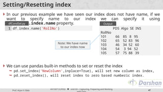
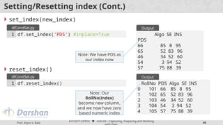
 Creating multiindexes is as simple as creating single index using set_index
method, only difference is in case of multiindexes we need to provide list of
indexes instead of a single string index, lets see and example for that
dfMulti =
pd.read_csv('MultiIndexDemo.csv')
dfMulti.set_index(['Col','Dep','Sem
'],inplace=True)
print(dfMulti)
1
2
3
dfMultiIndex.py
RN S1 S2 S3
Col Dep Sem
ABC CE 5 101 50 60
70
5 102 48 70
25
7 101 58 59
51
ME 5 101 30 35
39
5 102 50 90
48
Darshan CE 5 101 88 99
77
Output

51. Prof. Arjun V. Bala
#3150713 (PDS)  Unit 03 – Capturing, Preparing and Working
51
Multi-Index DataFrame (Cont.)
 Now we have multi-indexed DataFrame from which we can access data using
multiple index
 For Example
 Sub DataFrame for all the students of Darshan
 Sub DataFrame for Computer Engineering
students from Darshan
print(dfMulti.loc['Darshan'
])
1
dfGrabDarshanSt
u.py
RN S1 S2 S3
Dep Sem
CE 5 101 88 99 77
5 102 99 84 76
7 101 88 77 99
ME 5 101 44 88 99
Output (Darshan)
print(dfMulti.loc['Darshan','CE
'])
1
dfGrabDarshanCEStu.
py
RN S1 S2 S3
Sem
5 101 88 99 77
5 102 99 84 76
7 101 88 77 99
Output (Darshan->CE)

52. Prof. Arjun V. Bala
#3150713 (PDS)  Unit 03 – Capturing, Preparing and Working
52
Reading in Multiindexed DataFrame directly from CSV
 read_csv function of pandas provides easy way to create multi-indexed
DataFrame directly while fetching the CSV file.
dfMultiCSV =
pd.read_csv('MultiIndexDemo.c
sv',index_col=[0,1,2])
#for multi-index in cols we
can use header parameter
print(dfMultiCSV)
1
2
dfMultiIndex.py
RN S1 S2 S3
Col Dep Sem
ABC CE 5 101 50 60
70
5 102 48 70
25
7 101 58 59
51
ME 5 101 30 35
39
5 102 50 90
48
Darshan CE 5 101 88 99
77
5 102 99 84
Output

53. Prof. Arjun V. Bala
#3150713 (PDS)  Unit 03 – Capturing, Preparing and Working
53
Cross Sections in DataFrame
 The xs() function is used to get cross-section
from the Series/DataFrame.
 This method takes a key argument to select data
at a particular level of a MultiIndex.
 Syntax :
 Example :
DataFrame.xs(key, axis=0, level=None,
drop_level=True)
syntax
=== Parameters ===
key : label
axis : Axis to
retrieve cross section
level : level of key
drop_level : False if you
want to preserve the level
dfMultiCSV =
pd.read_csv('MultiIndexDemo.csv',
index_col=[0,1,2])
print(dfMultiCSV)
print(dfMultiCSV.xs('CE',axis=0,level='De
p'))
1
2
3
dfMultiIndex.py
RN S1 S2 S3
Col Dep Sem
ABC CE 5 101 50 60
70
5 102 48 70
25
7 101 58 59
51
ME 5 101 30 35
39
Output
RN S1 S2 S3
Col Sem
ABC 5 101 50 60 70
5 102 48 70 25
7 101 58 59 51
Darshan 5 101 88 99 77
5 102 99 84 76
7 101 88 77 99

54. Prof. Arjun V. Bala
#3150713 (PDS)  Unit 03 – Capturing, Preparing and Working
54
Dealing with Missing Data
 There are many methods by which we can deal with the missing data, some of
most commons are listed below,
 dropna, will drop (delete) the missing data (rows/cols)
 fillna, will fill specified values in place of missing data
 interpolate, will interpolate missing data and fill interpolated value in place of missing data.

55. Prof. Arjun V. Bala
#3150713 (PDS)  Unit 03 – Capturing, Preparing and Working
55
Groupby in Pandas
 Any groupby operation involves one of the
following operations on the original object.
They are
 Splitting the Object
 Applying a function
 Combining the results
 In many situations, we split the data into sets
and we apply some functionality on each
subset.
 we can perform the following operations
 Aggregation computing a summary statistic
−
 Transformation perform some group-specific
−
operation
 Filtration discarding the data with some
−
condition
 Basic ways to use of groupby method
 df.groupby('key')
Colleg
e
Enn
o
CP
I
Darsh
an
123 8.9
Darsh
an
124 9.2
Darsh
an
125 7.8
Darsh
an
128 8.7
ABC 211 5.6
ABC 212 6.2
ABC 215 3.2
ABC 218 4.2
XYZ 312 5.2
College Mean
CPI
Darshan 8.65
ABC 4.8
XYZ 5.83

56. Prof. Arjun V. Bala
#3150713 (PDS)  Unit 03 – Capturing, Preparing and Working
56
Groupby in Pandas (Cont.)
 Example : Listing all the groups
dfIPL =
pd.read_csv('IPLDataSet.csv')
print(dfIPL.groupby('Year').groups)
1
2
dfGroup.py
{2014: Int64Index([0, 2, 4,
9], dtype='int64'),
2015: Int64Index([1, 3, 5,
10], dtype='int64'),
2016: Int64Index([6, 8],
dtype='int64'),
2017: Int64Index([7, 11],
dtype='int64')}
Output

57. Prof. Arjun V. Bala
#3150713 (PDS)  Unit 03 – Capturing, Preparing and Working
57
Groupby in Pandas (Cont.)
 Example : Group by multiple columns
dfIPL =
pd.read_csv('IPLDataSet.csv')
print(dfIPL.groupby(['Year','Team']).gro
ups)
1
2
dfGroupMul.py
{(2014, 'Devils'):
Int64Index([2], dtype='int64'),
(2014, 'Kings'): Int64Index([4],
dtype='int64'),
(2014, 'Riders'):
Int64Index([0], dtype='int64'),
………
………
(2016, 'Riders'):
Int64Index([8], dtype='int64'),
(2017, 'Kings'): Int64Index([7],
dtype='int64'),
(2017, 'Riders'):
Int64Index([11], dtype='int64')}
Output

58. Prof. Arjun V. Bala
#3150713 (PDS)  Unit 03 – Capturing, Preparing and Working
58
Groupby in Pandas (Cont.)
 Example : Iterating through groups
dfIPL =
pd.read_csv('IPLDataSet.csv')
groupIPL = dfIPL.groupby('Year')
for name,group in groupIPL :
print(name)
print(group)
1
2
3
4
5
dfGroupIter.py
2014
Team Rank Year Points
0 Riders 1 2014 876
2 Devils 2 2014 863
4 Kings 3 2014 741
9 Royals 4 2014 701
2015
Team Rank Year Points
1 Riders 2 2015 789
3 Devils 3 2015 673
5 kings 4 2015 812
10 Royals 1 2015 804
2016
Team Rank Year Points
6 Kings 1 2016 756
8 Riders 2 2016 694
2017
Team Rank Year Points
7 Kings 1 2017 788
11 Riders 2 2017 690
Output

59. Prof. Arjun V. Bala
#3150713 (PDS)  Unit 03 – Capturing, Preparing and Working
59
Groupby in Pandas (Cont.)
 Example : Aggregating groups
dfSales =
pd.read_csv('SalesDataSet.csv')
print(dfSales.groupby(['YEAR_ID']).co
unt()['QUANTITYORDERED'])
print(dfSales.groupby(['YEAR_ID']).su
m()['QUANTITYORDERED'])
print(dfSales.groupby(['YEAR_ID']).me
an()['QUANTITYORDERED'])
1
2
3
4
dfGroupAgg.py
YEAR_ID
2003 1000
2004 1345
2005 478
Name: QUANTITYORDERED, dtype:
int64
YEAR_ID
2003 34612
2004 46824
2005 17631
Name: QUANTITYORDERED, dtype:
int64
YEAR_ID
2003 34.612000
2004 34.813383
2005 36.884937
Name: QUANTITYORDERED, dtype:
float64
Output

60. Prof. Arjun V. Bala
#3150713 (PDS)  Unit 03 – Capturing, Preparing and Working
60
Groupby in Pandas (Cont.)
 Example : Describe details
dfIPL =
pd.read_csv('IPLDataSet.csv')
print(dfIPL.groupby('Year').d
escribe()['Points'])
1
2
dfGroupDesc.py
count mean std min
25% 50% 75% max
Year
2014 4.0 795.25 87.439026
701.0 731.0 802.0 866.25 876.0
2015 4.0 769.50 65.035888
673.0 760.0 796.5 806.00 812.0
2016 2.0 725.00 43.840620
694.0 709.5 725.0 740.50 756.0
2017 2.0 739.00 69.296465
690.0 714.5 739.0 763.50 788.0
Output

61. Prof. Arjun V. Bala
#3150713 (PDS)  Unit 03 – Capturing, Preparing and Working
61
Concatenation in Pandas
 Concatenation basically glues together DataFrames.
 Keep in mind that dimensions should match along the axis you are
concatenating on.
 You can use pd.concat and pass in a list of DataFrames to concatenate
together:
 Note : We can use axis=1 parameter to concat columns.
dfCX =
pd.read_csv('CX_Marks.csv',index_col=0)
dfCY =
pd.read_csv('CY_Marks.csv',index_col=0)
dfCZ =
pd.read_csv('CZ_Marks.csv',index_col=0)
dfAllStudent = pd.concat([dfCX,dfCY,dfCZ])
print(dfAllStudent)
1
2
3
4
5
dfConcat.py
PDS Algo SE
101 50 55 60
102 70 80 61
103 55 89 70
104 58 96 85
201 77 96 63
202 44 78 32
203 55 85 21
204 69 66 54
301 11 75 88
302 22 48 77
303 33 59 68
304 44 55 62
Output

62. Prof. Arjun V. Bala
#3150713 (PDS)  Unit 03 – Capturing, Preparing and Working
62
Join in Pandas
 df.join() method will efficiently join multiple DataFrame objects by index(or
column specified) .
 some of important Parameters :
 dfOther : Right Data Frame
 on (Not recommended) : specify the column on which we want to join (Default is index)
 how : How to handle the operation of the two objects.
 left: use calling frame’s index (Default).
 right: use dfOther index.
 outer: form union of calling frame’s index with other’s index (or column if on is specified), and sort
it. lexicographically.
 inner: form intersection of calling frame’s index (or column if on is specified) with other’s index,
preserving the order of the calling’s one.

63. Prof. Arjun V. Bala
#3150713 (PDS)  Unit 03 – Capturing, Preparing and Working
63
Join in Pandas (Example)
dfINS =
pd.read_csv('INS_Marks.csv',index_col=0
)
dfLeftJoin = allStudent.join(dfINS)
print(dfLeftJoin)
dfRightJoin =
allStudent.join(dfINS,how='right')
print(dfRightJoin)
1
2
3
4
5
dfJoin.py
PDS Algo SE
INS
301 11 75 88
11
302 22 48 77
22
303 33 59 68
33
304 44 55 62
44
101 50 55 60
55
102 70 80 61
66
103 55 89 70
77
104 58 96 85
88
Output - 2
PDS Algo SE
INS
101 50 55 60
55.0
102 70 80 61
66.0
103 55 89 70
77.0
104 58 96 85
88.0
201 77 96 63
66.0
202 44 78 32
NaN
203 55 85 21
78.0
204 69 66 54
85.0
Output - 1

64. Prof. Arjun V. Bala
#3150713 (PDS)  Unit 03 – Capturing, Preparing and Working
64
Merge in Pandas
 Merge DataFrame or named Series objects with a database-style join.
 Similar to join method, but used when we want to join/merge with the columns
instead of index.
 some of important Parameters :
 dfOther : Right Data Frame
 on : specify the column on which we want to join (Default is index)
 left_on : specify the column of left Dataframe
 right_on : specify the column of right Dataframe
 how : How to handle the operation of the two objects.
 left: use calling frame’s index (Default).
 right: use dfOther index.
 outer: form union of calling frame’s index with other’s index (or column if on is specified), and sort
it. lexicographically.
 inner: form intersection of calling frame’s index (or column if on is specified) with other’s index,
preserving the order of the calling’s one.

65. Prof. Arjun V. Bala
#3150713 (PDS)  Unit 03 – Capturing, Preparing and Working
65
Merge in Pandas (Example)
m1 = pd.read_csv('Merge1.csv')
print(m1)
m2 = pd.read_csv('Merge2.csv')
print(m2)
m3 = m1.merge(m2,on='EnNo')
print(m3)
1
2
3
4
5
6
dfMerge.py
RollNo EnNo Name
0 101 11112222 Abc
1 102 11113333 Xyz
2 103 22224444 Def
EnNo PDS INS
0 11112222 50 60
1 11113333 60 70
RollNo EnNo Name PDS
INS
0 101 11112222 Abc 50
60
1 102 11113333 Xyz 60
70
Output

66. Prof. Arjun V. Bala
#3150713 (PDS)  Unit 03 – Capturing, Preparing and Working
66
Read CSV in Pandas
 read_csv() is used to read Comma Separated Values (CSV) file into a pandas
DataFrame.
 some of important Parameters :
 filePath : str, path object, or file-like object
 sep : separator (Default is comma)
 header: Row number(s) to use as the column names.
 index_col : index column(s) of the data frame.
dfINS =
pd.read_csv('Marks.csv',index_col=0,header=0)
print(dfINS)
1
2
readCSV.py
PDS Algo SE
INS
101 50 55 60
55.0
102 70 80 61
66.0
103 55 89 70
77.0
104 58 96 85
88.0
201 77 96 63
Output

67. Prof. Arjun V. Bala
#3150713 (PDS)  Unit 03 – Capturing, Preparing and Working
67
Read Excel in Pandas
 Read an Excel file into a pandas DataFrame.
 Supports xls, xlsx, xlsm, xlsb, odf, ods and odt file extensions read from a local
filesystem or URL. Supports an option to read a single sheet or a list of sheets.
 some of important Parameters :
 excelFile : str, bytes, ExcelFile, xlrd.Book, path object, or file-like object
 sheet_name : sheet no in integer or the name of the sheet, can have list of sheets.
 index_col : index column of the data frame.

68. Prof. Arjun V. Bala
#3150713 (PDS)  Unit 03 – Capturing, Preparing and Working
68
Read from MySQL Database
 We need two libraries for that,
 conda install sqlalchemy
 conda install pymysql
 After installing both the libraries, import create_engine from sqlalchemy
and import pymysql
 Then, create a database connection string and create engine using it.
from sqlalchemy import create_engine
import pymysql
1
2
importsForDB.p
y
db_connection_str = 'mysql+pymysql://username:password@host/dbname'
db_connection = create_engine(db_connection_str)
1
2
createEngine.py

69. Prof. Arjun V. Bala
#3150713 (PDS)  Unit 03 – Capturing, Preparing and Working
69
Read from MySQL Database (Cont.)
 After getting the engine, we can fire any sql query using pd.read_sql method.
 read_sql is a generic method which can be used to read from any sql
(MySQL,MSSQL, Oracle etc…)
df = pd.read_sql('SELECT * FROM cities', con=db_connection)
print(df)
1
2
readSQLDemo.p
y
CityID CityName CityDescription CityCode
0 1 Rajkot Rajkot Description here RJT
1 2 Ahemdabad Ahemdabad Description here ADI
2 3 Surat Surat Description here SRT
Output

70. Prof. Arjun V. Bala
#3150713 (PDS)  Unit 03 – Capturing, Preparing and Working
70
Web Scrapping using Beautiful Soup
 Beautiful Soup is a library that makes it easy to scrape information from web
pages.
 It sits atop an HTML or XML parser, providing Pythonic idioms for iterating,
searching, and modifying the parse tree.
import requests
import bs4
req =
requests.get('https://www.darshan.ac.in/DIET/CE/Facu
lty')
soup = bs4.BeautifulSoup(req.text,'lxml')
allFaculty = soup.select('body > main > section:nth-
child(5) > div > div > div.col-lg-8.col-xl-9 > div >
div')
for fac in allFaculty :
allSpans = fac.select('h2>a')
print(allSpans[0].text.strip())
1
2
3
4
5
6
7
8
webScrap.py Dr. Gopi Sanghani
Dr. Nilesh
Gambhava
Dr. Pradyumansinh
Jadeja
Prof. Hardik Doshi
Prof. Maulik Trivedi
Prof. Dixita
Kagathara
Prof. Firoz
Sherasiya
Prof. Rupesh
Vaishnav
Prof. Swati Sharma
Prof. Arjun Bala
Output