Using MapReduce for
Large-scale Medical Image
Analysis
HISB 2012
Presented by : Roger Schaer - HES-SO Valais
Summary
Introduction
Methods
Results & Interpretation
Conclusions
2
Introduction
Introduction
Exponential growth of imaging data (past 20 years)
Year
Amountofimagesproduced
perdayattheHUG
4
Introduction (continued)
Mainly caused by :
Modern imaging techniques (3D, 4D) : Large files !
Large collections (available on the Internet)
Increasingly complex algorithms make processing
this data more challenging
Requires a lot of computation power, storage and
network bandwidth
5
Introduction (continued)
Flexible and scalable infrastructures are needed
Several approaches exist :
Single, powerful machine
Local cluster / grid
Alternative infrastructures (Graphics cards)
Cloud computing solutions
First two approaches have been tested and compared
6
Introduction (continued)
3 large-scale medical image processing use cases
Parameter optimization for Support Vector Machines
Content-based image feature extraction & indexing
3D texture feature extraction using the Riesz
transform
NOTE : I mostly handled the infrastructure
aspects !
7
Methods
Methods
MapReduce
Hadoop Cluster
Support Vector Machines
Image Indexing
Solid 3D Texture Analysis Using the Riesz Transform
9
MapReduce
MapReduce is a programming model
Developed by Google
Map Phase : Key/Value pair input, Intermediate
output
Reduce phase : For each intermediate key, process
the list of associated values
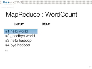
Trivial example : Word Count application
10
MapReduce : WordCount
11
MapReduce : WordCount
INPUT
11
MapReduce : WordCount
#1 hello world
#2 goodbye world
#3 hello hadoop
#4 bye hadoop
...
INPUT
11
MapReduce : WordCount
#1 hello world
#2 goodbye world
#3 hello hadoop
#4 bye hadoop
...
INPUT MAP
11
MapReduce : WordCount
#1 hello world
#2 goodbye world
#3 hello hadoop
#4 bye hadoop
...
INPUT MAP
11
MapReduce : WordCount
#1 hello world
#2 goodbye world
#3 hello hadoop
#4 bye hadoop
...
hello 1
INPUT MAP
11
MapReduce : WordCount
#1 hello world
#2 goodbye world
#3 hello hadoop
#4 bye hadoop
...
hello 1
world 1
INPUT MAP
11
MapReduce : WordCount
#1 hello world
#2 goodbye world
#3 hello hadoop
#4 bye hadoop
...
hello 1
world 1
INPUT MAP
11
MapReduce : WordCount
#1 hello world
#2 goodbye world
#3 hello hadoop
#4 bye hadoop
...
hello 1
world 1
goodbye 1
INPUT MAP
11
MapReduce : WordCount
#1 hello world
#2 goodbye world
#3 hello hadoop
#4 bye hadoop
...
hello 1
world 1
goodbye 1
world 1
INPUT MAP
11
MapReduce : WordCount
#1 hello world
#2 goodbye world
#3 hello hadoop
#4 bye hadoop
...
hello 1
world 1
goodbye 1
world 1
INPUT MAP
11
MapReduce : WordCount
#1 hello world
#2 goodbye world
#3 hello hadoop
#4 bye hadoop
...
hello 1
world 1
goodbye 1
world 1
hello 1
INPUT MAP
11
MapReduce : WordCount
#1 hello world
#2 goodbye world
#3 hello hadoop
#4 bye hadoop
...
hello 1
world 1
goodbye 1
world 1
hello 1
hadoop 1
INPUT MAP
11
MapReduce : WordCount
#1 hello world
#2 goodbye world
#3 hello hadoop
#4 bye hadoop
...
hello 1
world 1
goodbye 1
world 1
hello 1
hadoop 1
INPUT MAP
11
MapReduce : WordCount
#1 hello world
#2 goodbye world
#3 hello hadoop
#4 bye hadoop
...
hello 1
world 1
goodbye 1
world 1
hello 1
hadoop 1
bye 1
INPUT MAP
11
MapReduce : WordCount
#1 hello world
#2 goodbye world
#3 hello hadoop
#4 bye hadoop
...
hello 1
world 1
goodbye 1
world 1
hello 1
hadoop 1
bye 1
hadoop 1
INPUT MAP
11
MapReduce : WordCount
#1 hello world
#2 goodbye world
#3 hello hadoop
#4 bye hadoop
...
hello 1
world 1
goodbye 1
world 1
hello 1
hadoop 1
bye 1
hadoop 1
INPUT MAP REDUCE
11
MapReduce : WordCount
#1 hello world
#2 goodbye world
#3 hello hadoop
#4 bye hadoop
...
hello 1
world 1
goodbye 1
world 1
hello 1
hadoop 1
bye 1
hadoop 1
INPUT MAP REDUCE
11
MapReduce : WordCount
#1 hello world
#2 goodbye world
#3 hello hadoop
#4 bye hadoop
...
hello 1
world 1
goodbye 1
world 1
hello 1
hadoop 1
bye 1
hadoop 1
INPUT MAP REDUCE
hello 2
11
MapReduce : WordCount
#1 hello world
#2 goodbye world
#3 hello hadoop
#4 bye hadoop
...
hello 1
world 1
goodbye 1
world 1
hello 1
hadoop 1
bye 1
hadoop 1
INPUT MAP REDUCE
hello 2
11
MapReduce : WordCount
#1 hello world
#2 goodbye world
#3 hello hadoop
#4 bye hadoop
...
hello 1
world 1
goodbye 1
world 1
hello 1
hadoop 1
bye 1
hadoop 1
INPUT MAP REDUCE
hello 2
world 2
11
MapReduce : WordCount
#1 hello world
#2 goodbye world
#3 hello hadoop
#4 bye hadoop
...
hello 1
world 1
goodbye 1
world 1
hello 1
hadoop 1
bye 1
hadoop 1
INPUT MAP REDUCE
hello 2
world 2
11
MapReduce : WordCount
#1 hello world
#2 goodbye world
#3 hello hadoop
#4 bye hadoop
...
hello 1
world 1
goodbye 1
world 1
hello 1
hadoop 1
bye 1
hadoop 1
INPUT MAP REDUCE
hello 2
world 2
goodbye 1
11
MapReduce : WordCount
#1 hello world
#2 goodbye world
#3 hello hadoop
#4 bye hadoop
...
hello 1
world 1
goodbye 1
world 1
hello 1
hadoop 1
bye 1
hadoop 1
INPUT MAP REDUCE
hello 2
world 2
goodbye 1
11
MapReduce : WordCount
#1 hello world
#2 goodbye world
#3 hello hadoop
#4 bye hadoop
...
hello 1
world 1
goodbye 1
world 1
hello 1
hadoop 1
bye 1
hadoop 1
INPUT MAP REDUCE
hello 2
world 2
goodbye 1
hadoop 2
11
MapReduce : WordCount
#1 hello world
#2 goodbye world
#3 hello hadoop
#4 bye hadoop
...
hello 1
world 1
goodbye 1
world 1
hello 1
hadoop 1
bye 1
hadoop 1
INPUT MAP REDUCE
hello 2
world 2
goodbye 1
hadoop 2
11
MapReduce : WordCount
#1 hello world
#2 goodbye world
#3 hello hadoop
#4 bye hadoop
...
hello 1
world 1
goodbye 1
world 1
hello 1
hadoop 1
bye 1
hadoop 1
INPUT MAP REDUCE
hello 2
world 2
goodbye 1
hadoop 2
bye 1
11
Hadoop
Apache’s implementation of MapReduce
Consists of
Distributed storage system : HDFS
Execution framework : Hadoop MapReduce
Master node which orchestrates the task distribution
Worker nodes which perform the tasks
Typical node runs a DataNode and TaskTracker
12
Support Vector Machines
Computes a decision boundary (hyperplane) that
separates inputs of different classes represented in a
given feature space transformed by a given kernel
The values of two parameters need to be adapted to
the data:
Cost C of errors
σ of the Gaussian kernel
13
Support Vector Machines
Computes a decision boundary (hyperplane) that
separates inputs of different classes represented in a
given feature space transformed by a given kernel
The values of two parameters need to be adapted to
the data:
Cost C of errors
σ of the Gaussian kernel
0
5
10
15
20
0 5 10 15 20 13
Support Vector Machines
Computes a decision boundary (hyperplane) that
separates inputs of different classes represented in a
given feature space transformed by a given kernel
The values of two parameters need to be adapted to
the data:
Cost C of errors
σ of the Gaussian kernel
0
5
10
15
20
0 5 10 15 20
?
13
Support Vector Machines
Computes a decision boundary (hyperplane) that
separates inputs of different classes represented in a
given feature space transformed by a given kernel
The values of two parameters need to be adapted to
the data:
Cost C of errors
σ of the Gaussian kernel
0
5
10
15
20
0 5 10 15 20 13
SVM (continued)
Goal : find optimal value couple (C, σ) to train a SVM
Allowing best classification performance of 5 lung
texture patterns
Execution on 1 PC (without Hadoop) can take weeks
Due to extensive leave-one-patient-out cross-
validation with 86 patients
Parallelization : Split job by parameter value couples 14
Image Indexing
Vocabulary
File
Image Files
Feature
Extractor
Feature Vectors
Files
Bag of Visual
Words Factory
Index File
Two phases
Extract features from
images
Construct bags of
visual words by
quantization
Component-based /
Monolithic approaches
Parallelization : Each task
processes N images 15
Image Indexing
Vocabulary
File
Image Files
Feature
Extractor
Feature Vectors
Files
Bag of Visual
Words Factory
Index File
Two phases
Extract features from
images
Construct bags of
visual words by
quantization
Component-based /
Monolithic approaches
Parallelization : Each task
processes N images 15
Feature
Extractor
+
Bag of
Visual
Words
Factory
3D Texture Analysis (Riesz)
Features are extracted from 3D images (see below)
Parallelization : Each task processes N images
16
Results & Interpretation
Hadoop Cluster
Minimally invasive setup (>=2 free cores per node)
18
Support Vector Machines
Optimization : Longer tasks = bad performance
Because the optimization of the hyperplane is more
difficult to compute (more iterations needed)
After 2 patients (out of 86), check if : ti ≥ F · tref.
If time exceeds average (+margin), terminate task
19
Support Vector Machines
Black : tasks to be interrupted by the new algorithm
Optimized algorithm : ~50h → ~9h15min
All the best tasks (highest accuracy) are not killed 20
σ (Sigma)
C
(Cost)
Accuracy(%)
Image Indexing
1K IMAGES
Shows the calculation time in function of the # of tasks
Both experiments were executed using hadoop
Once on a single computer, then on our cluster of PCs 21
Image Indexing
1K IMAGES 10K IMAGES
Shows the calculation time in function of the # of tasks
Both experiments were executed using hadoop
Once on a single computer, then on our cluster of PCs 21
Image Indexing
1K IMAGES 10K IMAGES 100K IMAGES
Shows the calculation time in function of the # of tasks
Both experiments were executed using hadoop
Once on a single computer, then on our cluster of PCs 21
Riesz 3D
Particularity : code was a series of Matlab® scripts
Instead of rewriting the whole application :
Used Hadoop streaming feature (uses stdin/stdout)
To maximize scalability, GNU Octave was used
Great compatibility between Matlab® and Octave
22
Riesz 3D
Particularity : code was a series of Matlab® scripts
Instead of rewriting the whole application :
Used Hadoop streaming feature (uses stdin/stdout)
To maximize scalability, GNU Octave was used
Great compatibility between Matlab® and Octave
RESULTS
1 task (no Hadoop) 42 tasks (idle) 42 tasks (normal)
131h32m42s 6h29m51s 5h51m31s
22
Conclusions
Conclusions
MapReduce is
Flexible (worked with very varied use cases)
Easy to use (2-phase programming model is simple)
Efficient (>=20x speedup for all use cases)
Hadoop is
Easy to deploy & manage
User-friendly (nice Web UIs)
24
Conclusions (continued)
Speedups for the different use cases
SVMs
Image
Indexing
3D Feature
Extraction
Single task 990h* 21h* 131h30
42 tasks on
hadoop
50h / 9h15** 1h 5h50
Speedup 20x / 107x** 21x 22.5x
* estimation ** using the optimized algorithm 25
Lessons Learned
It is important to use physically distributed resources
Overloading a single machine hurts performance
Data locality notably speeds up jobs
Not every application is infinitely scalable
Performance improvements level off at some point
26
Future work
Take it to the next level : The Cloud
Amazon Elastic Cloud Compute (IaaS)
Amazon Elastic MapReduce (PaaS)
Cloudbursting
Use both local resources + Cloud (for peak usage)
27
Thank you ! Questions ?

Using MapReduce for Large–scale Medical Image Analysis

  • 1.
    Using MapReduce for Large-scaleMedical Image Analysis HISB 2012 Presented by : Roger Schaer - HES-SO Valais
  • 2.
  • 3.
  • 4.
    Introduction Exponential growth ofimaging data (past 20 years) Year Amountofimagesproduced perdayattheHUG 4
  • 5.
    Introduction (continued) Mainly causedby : Modern imaging techniques (3D, 4D) : Large files ! Large collections (available on the Internet) Increasingly complex algorithms make processing this data more challenging Requires a lot of computation power, storage and network bandwidth 5
  • 6.
    Introduction (continued) Flexible andscalable infrastructures are needed Several approaches exist : Single, powerful machine Local cluster / grid Alternative infrastructures (Graphics cards) Cloud computing solutions First two approaches have been tested and compared 6
  • 7.
    Introduction (continued) 3 large-scalemedical image processing use cases Parameter optimization for Support Vector Machines Content-based image feature extraction & indexing 3D texture feature extraction using the Riesz transform NOTE : I mostly handled the infrastructure aspects ! 7
  • 8.
  • 9.
    Methods MapReduce Hadoop Cluster Support VectorMachines Image Indexing Solid 3D Texture Analysis Using the Riesz Transform 9
  • 10.
    MapReduce MapReduce is aprogramming model Developed by Google Map Phase : Key/Value pair input, Intermediate output Reduce phase : For each intermediate key, process the list of associated values Trivial example : Word Count application 10
  • 11.
  • 12.
  • 13.
    MapReduce : WordCount #1hello world #2 goodbye world #3 hello hadoop #4 bye hadoop ... INPUT 11
  • 14.
    MapReduce : WordCount #1hello world #2 goodbye world #3 hello hadoop #4 bye hadoop ... INPUT MAP 11
  • 15.
    MapReduce : WordCount #1hello world #2 goodbye world #3 hello hadoop #4 bye hadoop ... INPUT MAP 11
  • 16.
    MapReduce : WordCount #1hello world #2 goodbye world #3 hello hadoop #4 bye hadoop ... hello 1 INPUT MAP 11
  • 17.
    MapReduce : WordCount #1hello world #2 goodbye world #3 hello hadoop #4 bye hadoop ... hello 1 world 1 INPUT MAP 11
  • 18.
    MapReduce : WordCount #1hello world #2 goodbye world #3 hello hadoop #4 bye hadoop ... hello 1 world 1 INPUT MAP 11
  • 19.
    MapReduce : WordCount #1hello world #2 goodbye world #3 hello hadoop #4 bye hadoop ... hello 1 world 1 goodbye 1 INPUT MAP 11
  • 20.
    MapReduce : WordCount #1hello world #2 goodbye world #3 hello hadoop #4 bye hadoop ... hello 1 world 1 goodbye 1 world 1 INPUT MAP 11
  • 21.
    MapReduce : WordCount #1hello world #2 goodbye world #3 hello hadoop #4 bye hadoop ... hello 1 world 1 goodbye 1 world 1 INPUT MAP 11
  • 22.
    MapReduce : WordCount #1hello world #2 goodbye world #3 hello hadoop #4 bye hadoop ... hello 1 world 1 goodbye 1 world 1 hello 1 INPUT MAP 11
  • 23.
    MapReduce : WordCount #1hello world #2 goodbye world #3 hello hadoop #4 bye hadoop ... hello 1 world 1 goodbye 1 world 1 hello 1 hadoop 1 INPUT MAP 11
  • 24.
    MapReduce : WordCount #1hello world #2 goodbye world #3 hello hadoop #4 bye hadoop ... hello 1 world 1 goodbye 1 world 1 hello 1 hadoop 1 INPUT MAP 11
  • 25.
    MapReduce : WordCount #1hello world #2 goodbye world #3 hello hadoop #4 bye hadoop ... hello 1 world 1 goodbye 1 world 1 hello 1 hadoop 1 bye 1 INPUT MAP 11
  • 26.
    MapReduce : WordCount #1hello world #2 goodbye world #3 hello hadoop #4 bye hadoop ... hello 1 world 1 goodbye 1 world 1 hello 1 hadoop 1 bye 1 hadoop 1 INPUT MAP 11
  • 27.
    MapReduce : WordCount #1hello world #2 goodbye world #3 hello hadoop #4 bye hadoop ... hello 1 world 1 goodbye 1 world 1 hello 1 hadoop 1 bye 1 hadoop 1 INPUT MAP REDUCE 11
  • 28.
    MapReduce : WordCount #1hello world #2 goodbye world #3 hello hadoop #4 bye hadoop ... hello 1 world 1 goodbye 1 world 1 hello 1 hadoop 1 bye 1 hadoop 1 INPUT MAP REDUCE 11
  • 29.
    MapReduce : WordCount #1hello world #2 goodbye world #3 hello hadoop #4 bye hadoop ... hello 1 world 1 goodbye 1 world 1 hello 1 hadoop 1 bye 1 hadoop 1 INPUT MAP REDUCE hello 2 11
  • 30.
    MapReduce : WordCount #1hello world #2 goodbye world #3 hello hadoop #4 bye hadoop ... hello 1 world 1 goodbye 1 world 1 hello 1 hadoop 1 bye 1 hadoop 1 INPUT MAP REDUCE hello 2 11
  • 31.
    MapReduce : WordCount #1hello world #2 goodbye world #3 hello hadoop #4 bye hadoop ... hello 1 world 1 goodbye 1 world 1 hello 1 hadoop 1 bye 1 hadoop 1 INPUT MAP REDUCE hello 2 world 2 11
  • 32.
    MapReduce : WordCount #1hello world #2 goodbye world #3 hello hadoop #4 bye hadoop ... hello 1 world 1 goodbye 1 world 1 hello 1 hadoop 1 bye 1 hadoop 1 INPUT MAP REDUCE hello 2 world 2 11
  • 33.
    MapReduce : WordCount #1hello world #2 goodbye world #3 hello hadoop #4 bye hadoop ... hello 1 world 1 goodbye 1 world 1 hello 1 hadoop 1 bye 1 hadoop 1 INPUT MAP REDUCE hello 2 world 2 goodbye 1 11
  • 34.
    MapReduce : WordCount #1hello world #2 goodbye world #3 hello hadoop #4 bye hadoop ... hello 1 world 1 goodbye 1 world 1 hello 1 hadoop 1 bye 1 hadoop 1 INPUT MAP REDUCE hello 2 world 2 goodbye 1 11
  • 35.
    MapReduce : WordCount #1hello world #2 goodbye world #3 hello hadoop #4 bye hadoop ... hello 1 world 1 goodbye 1 world 1 hello 1 hadoop 1 bye 1 hadoop 1 INPUT MAP REDUCE hello 2 world 2 goodbye 1 hadoop 2 11
  • 36.
    MapReduce : WordCount #1hello world #2 goodbye world #3 hello hadoop #4 bye hadoop ... hello 1 world 1 goodbye 1 world 1 hello 1 hadoop 1 bye 1 hadoop 1 INPUT MAP REDUCE hello 2 world 2 goodbye 1 hadoop 2 11
  • 37.
    MapReduce : WordCount #1hello world #2 goodbye world #3 hello hadoop #4 bye hadoop ... hello 1 world 1 goodbye 1 world 1 hello 1 hadoop 1 bye 1 hadoop 1 INPUT MAP REDUCE hello 2 world 2 goodbye 1 hadoop 2 bye 1 11
  • 38.
    Hadoop Apache’s implementation ofMapReduce Consists of Distributed storage system : HDFS Execution framework : Hadoop MapReduce Master node which orchestrates the task distribution Worker nodes which perform the tasks Typical node runs a DataNode and TaskTracker 12
  • 39.
    Support Vector Machines Computesa decision boundary (hyperplane) that separates inputs of different classes represented in a given feature space transformed by a given kernel The values of two parameters need to be adapted to the data: Cost C of errors σ of the Gaussian kernel 13
  • 40.
    Support Vector Machines Computesa decision boundary (hyperplane) that separates inputs of different classes represented in a given feature space transformed by a given kernel The values of two parameters need to be adapted to the data: Cost C of errors σ of the Gaussian kernel 0 5 10 15 20 0 5 10 15 20 13
  • 41.
    Support Vector Machines Computesa decision boundary (hyperplane) that separates inputs of different classes represented in a given feature space transformed by a given kernel The values of two parameters need to be adapted to the data: Cost C of errors σ of the Gaussian kernel 0 5 10 15 20 0 5 10 15 20 13
  • 42.
    Support Vector Machines Computesa decision boundary (hyperplane) that separates inputs of different classes represented in a given feature space transformed by a given kernel The values of two parameters need to be adapted to the data: Cost C of errors σ of the Gaussian kernel 0 5 10 15 20 0 5 10 15 20 13
  • 43.
    Support Vector Machines Computesa decision boundary (hyperplane) that separates inputs of different classes represented in a given feature space transformed by a given kernel The values of two parameters need to be adapted to the data: Cost C of errors σ of the Gaussian kernel 0 5 10 15 20 0 5 10 15 20 ? 13
  • 44.
    Support Vector Machines Computesa decision boundary (hyperplane) that separates inputs of different classes represented in a given feature space transformed by a given kernel The values of two parameters need to be adapted to the data: Cost C of errors σ of the Gaussian kernel 0 5 10 15 20 0 5 10 15 20 13
  • 45.
    SVM (continued) Goal :find optimal value couple (C, σ) to train a SVM Allowing best classification performance of 5 lung texture patterns Execution on 1 PC (without Hadoop) can take weeks Due to extensive leave-one-patient-out cross- validation with 86 patients Parallelization : Split job by parameter value couples 14
  • 46.
    Image Indexing Vocabulary File Image Files Feature Extractor FeatureVectors Files Bag of Visual Words Factory Index File Two phases Extract features from images Construct bags of visual words by quantization Component-based / Monolithic approaches Parallelization : Each task processes N images 15
  • 47.
    Image Indexing Vocabulary File Image Files Feature Extractor FeatureVectors Files Bag of Visual Words Factory Index File Two phases Extract features from images Construct bags of visual words by quantization Component-based / Monolithic approaches Parallelization : Each task processes N images 15 Feature Extractor + Bag of Visual Words Factory
  • 48.
    3D Texture Analysis(Riesz) Features are extracted from 3D images (see below) Parallelization : Each task processes N images 16
  • 49.
  • 50.
    Hadoop Cluster Minimally invasivesetup (>=2 free cores per node) 18
  • 51.
    Support Vector Machines Optimization: Longer tasks = bad performance Because the optimization of the hyperplane is more difficult to compute (more iterations needed) After 2 patients (out of 86), check if : ti ≥ F · tref. If time exceeds average (+margin), terminate task 19
  • 52.
    Support Vector Machines Black: tasks to be interrupted by the new algorithm Optimized algorithm : ~50h → ~9h15min All the best tasks (highest accuracy) are not killed 20 σ (Sigma) C (Cost) Accuracy(%)
  • 53.
    Image Indexing 1K IMAGES Showsthe calculation time in function of the # of tasks Both experiments were executed using hadoop Once on a single computer, then on our cluster of PCs 21
  • 54.
    Image Indexing 1K IMAGES10K IMAGES Shows the calculation time in function of the # of tasks Both experiments were executed using hadoop Once on a single computer, then on our cluster of PCs 21
  • 55.
    Image Indexing 1K IMAGES10K IMAGES 100K IMAGES Shows the calculation time in function of the # of tasks Both experiments were executed using hadoop Once on a single computer, then on our cluster of PCs 21
  • 56.
    Riesz 3D Particularity :code was a series of Matlab® scripts Instead of rewriting the whole application : Used Hadoop streaming feature (uses stdin/stdout) To maximize scalability, GNU Octave was used Great compatibility between Matlab® and Octave 22
  • 57.
    Riesz 3D Particularity :code was a series of Matlab® scripts Instead of rewriting the whole application : Used Hadoop streaming feature (uses stdin/stdout) To maximize scalability, GNU Octave was used Great compatibility between Matlab® and Octave RESULTS 1 task (no Hadoop) 42 tasks (idle) 42 tasks (normal) 131h32m42s 6h29m51s 5h51m31s 22
  • 58.
  • 59.
    Conclusions MapReduce is Flexible (workedwith very varied use cases) Easy to use (2-phase programming model is simple) Efficient (>=20x speedup for all use cases) Hadoop is Easy to deploy & manage User-friendly (nice Web UIs) 24
  • 60.
    Conclusions (continued) Speedups forthe different use cases SVMs Image Indexing 3D Feature Extraction Single task 990h* 21h* 131h30 42 tasks on hadoop 50h / 9h15** 1h 5h50 Speedup 20x / 107x** 21x 22.5x * estimation ** using the optimized algorithm 25
  • 61.
    Lessons Learned It isimportant to use physically distributed resources Overloading a single machine hurts performance Data locality notably speeds up jobs Not every application is infinitely scalable Performance improvements level off at some point 26
  • 62.
    Future work Take itto the next level : The Cloud Amazon Elastic Cloud Compute (IaaS) Amazon Elastic MapReduce (PaaS) Cloudbursting Use both local resources + Cloud (for peak usage) 27
  • 63.
    Thank you !Questions ?