Chapter 2 of Dr. Rashmita Saran's document covers numerical descriptive measures, including classification of data (qualitative and quantitative), data representation methods, frequency distribution, and key descriptive statistics (mean, median, mode, standard deviation). It explains various types of data, the importance of accuracy in data collection, and the scales of measurement (nominal, ordinal, interval, and ratio). The chapter also discusses methods for organizing data and calculating measures of central tendency and dispersion.

1. Chapter 2
Numerical Descriptive Measures
Dr. Rashmita Saran
Department of Mktg & Strategy
IBS Hyderabad

2. Outline
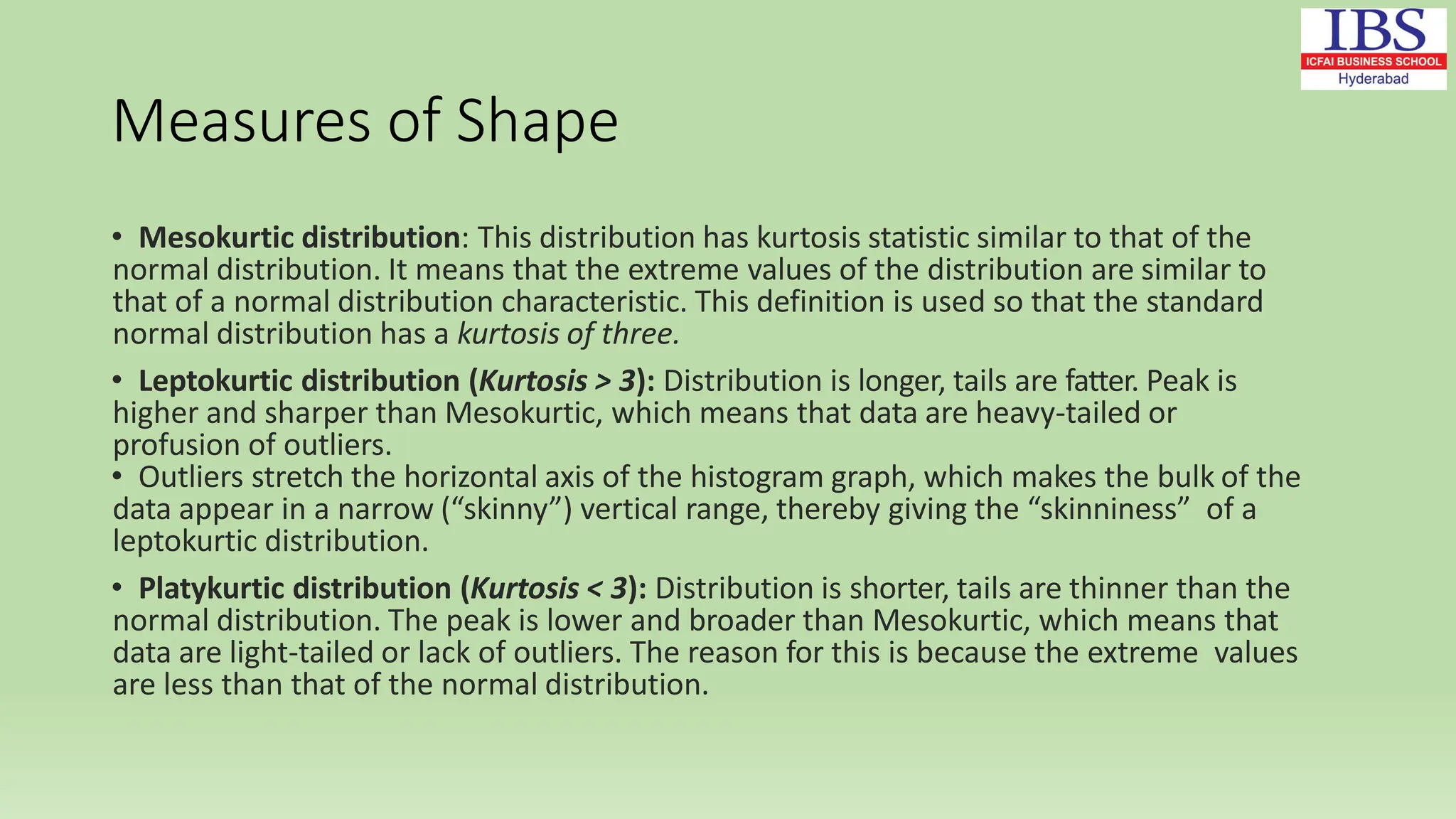
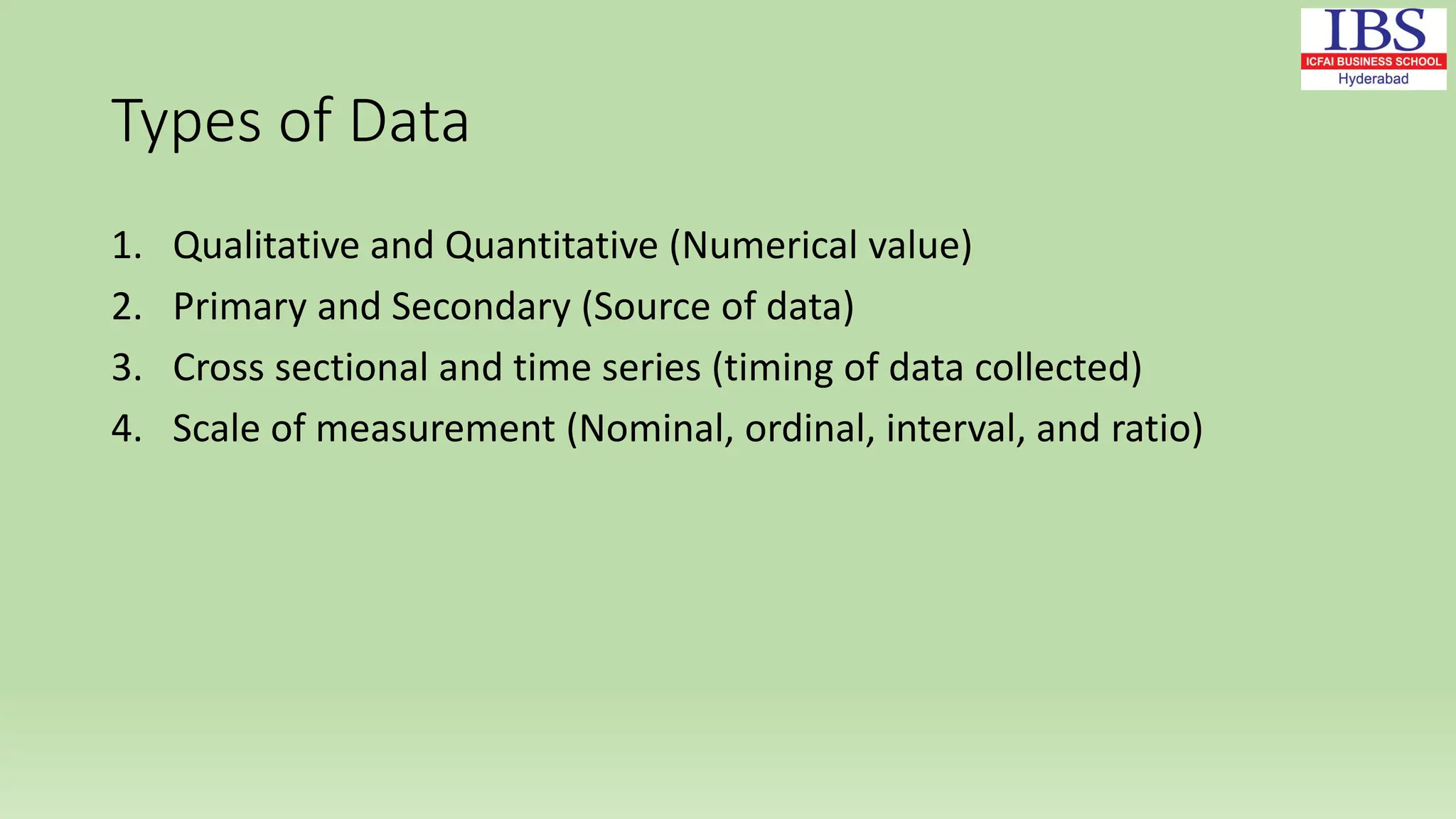
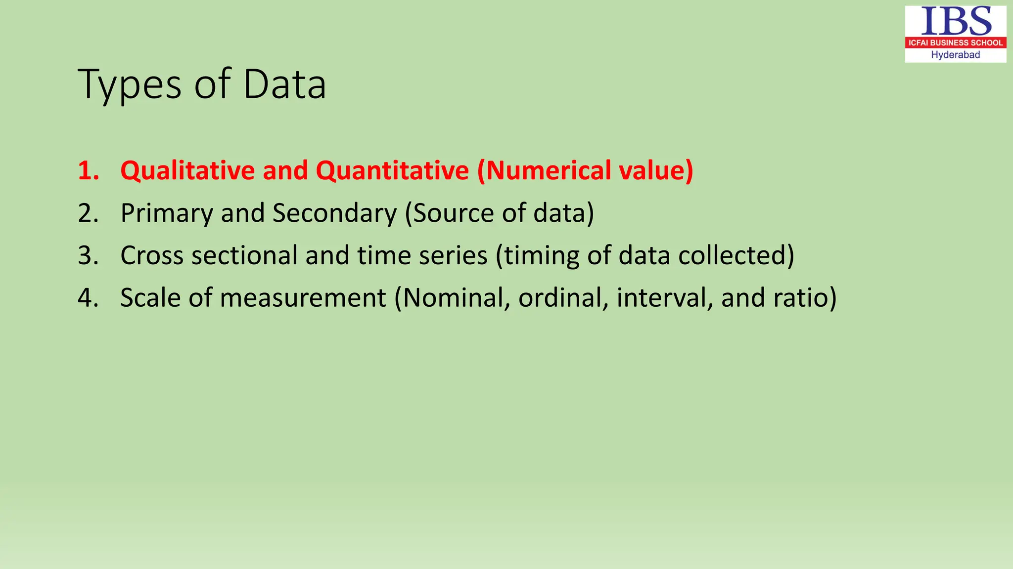
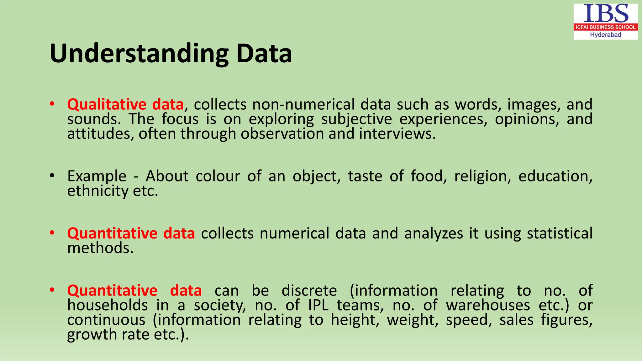
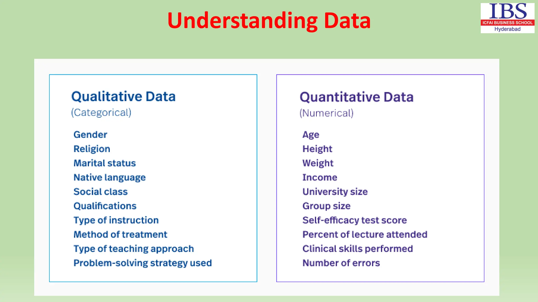
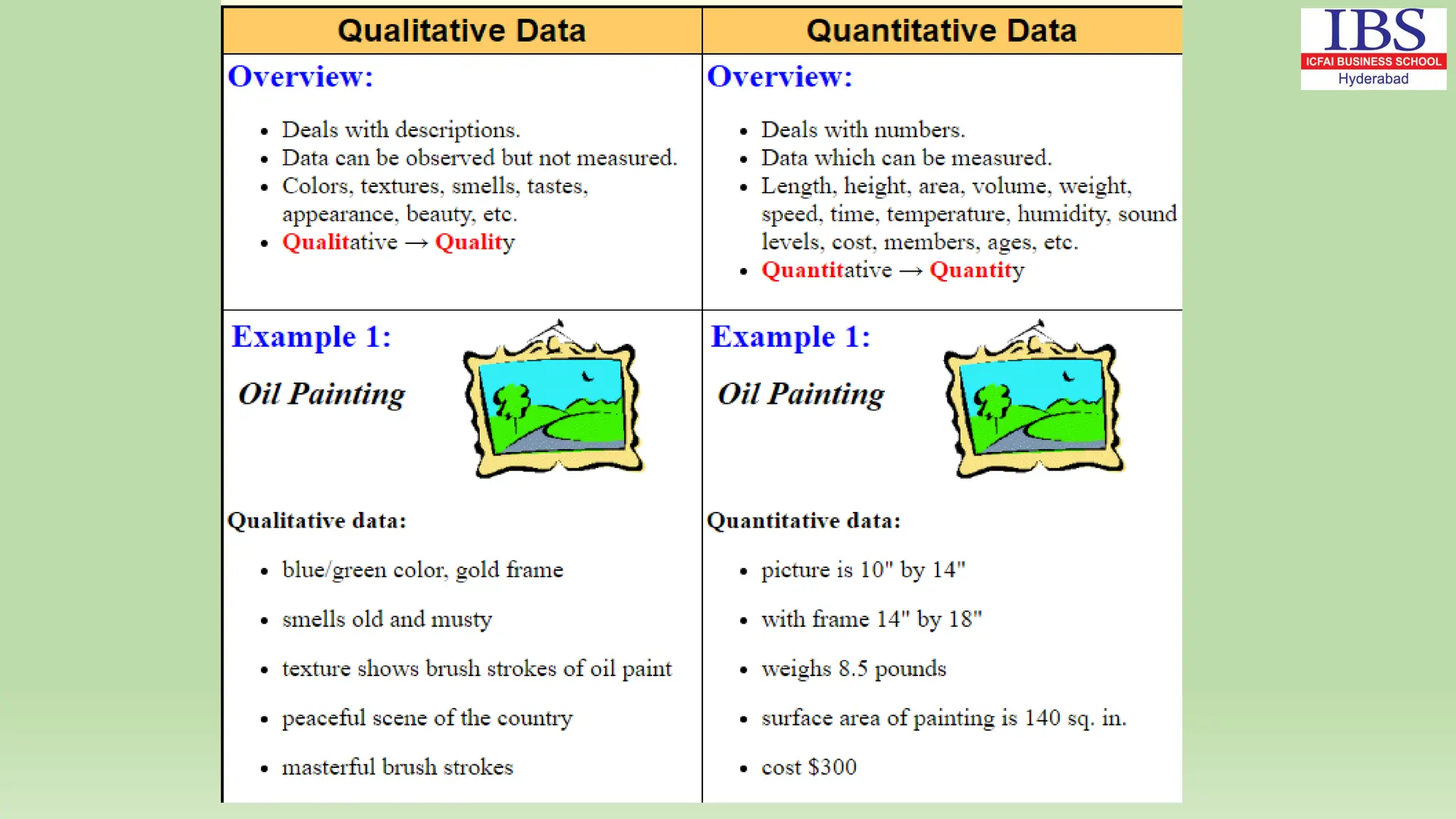
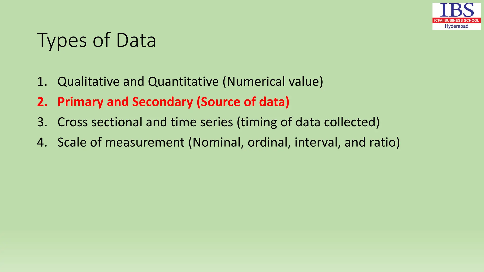
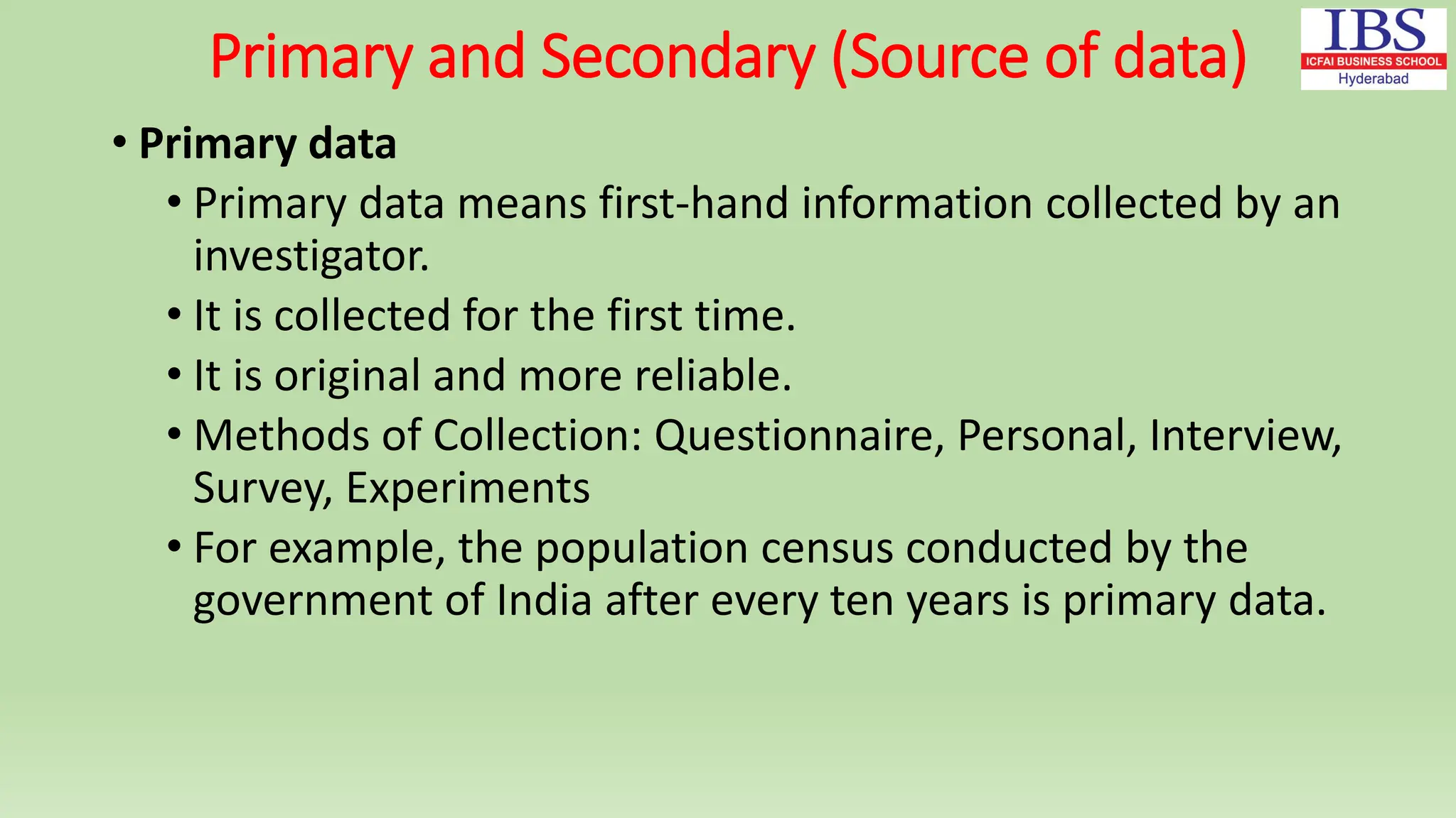
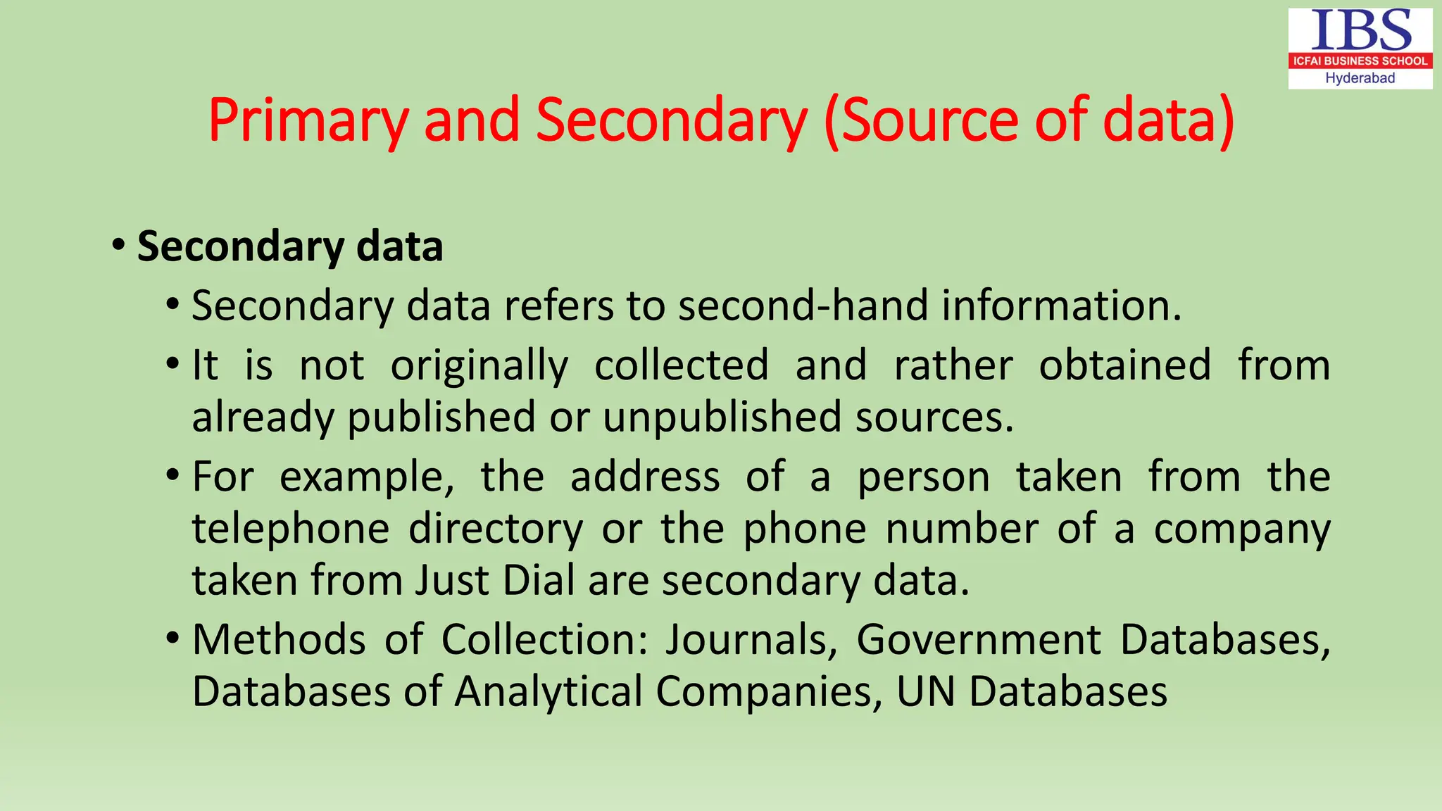
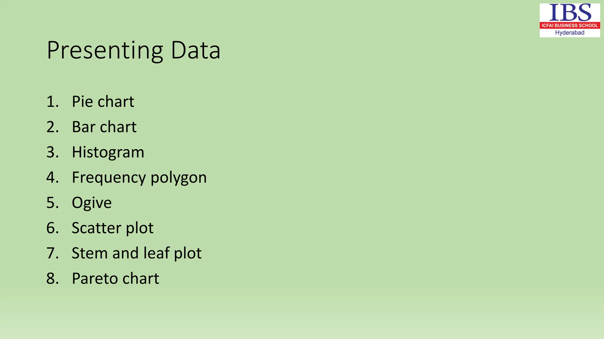
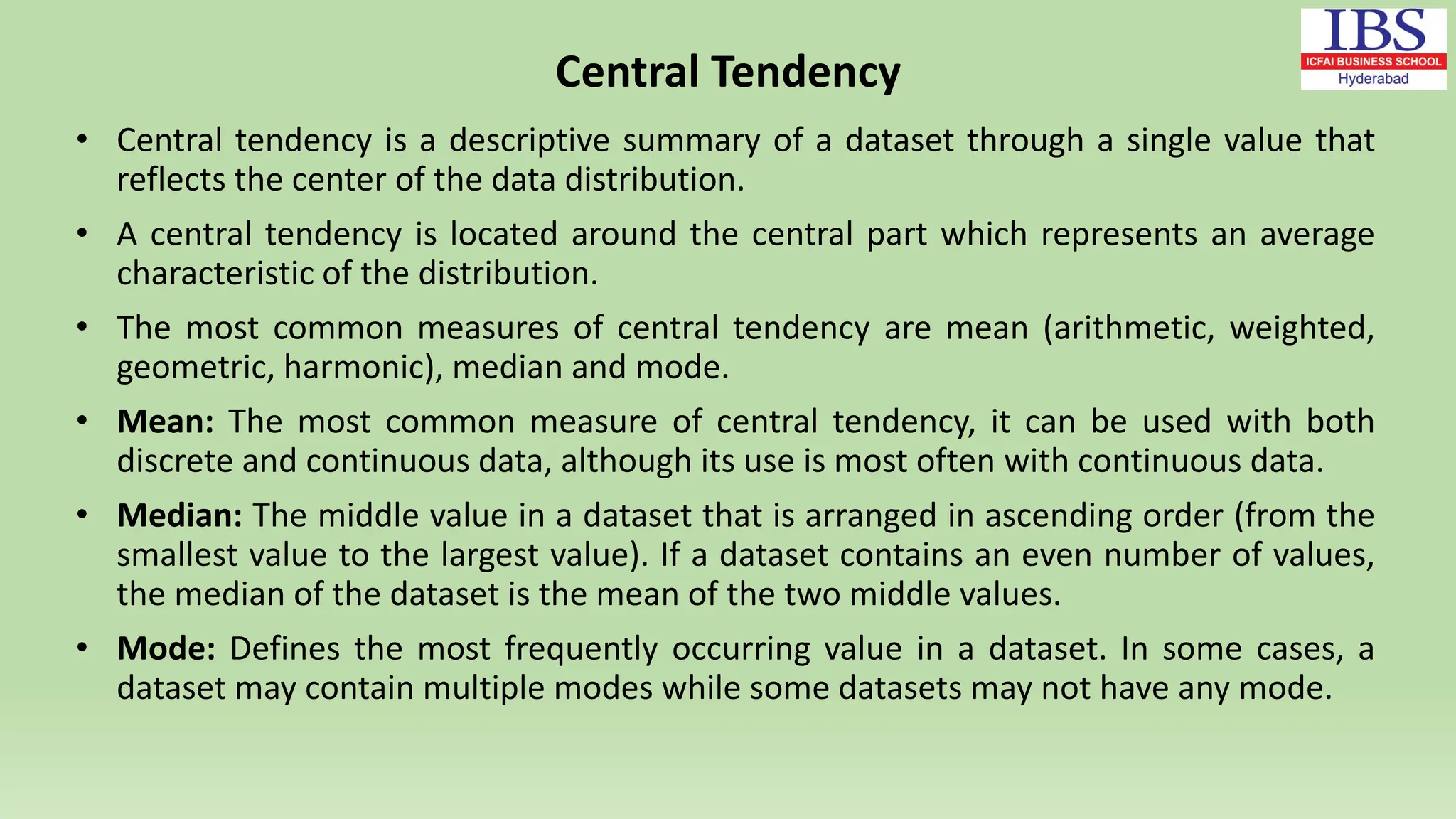
• Classification of Data
•Data Representation
• Frequency distribution
•Descriptive Statistics[Mean, Median, Mode, Standard
deviation]
• Outliers
• Skewness & Kurtosis

3. • Classification of data: Qualitative Data (Nominal Data and Ordinal Data)
and
• Quantitative Data (Discrete Data and Continuous Data)
• Descriptive statistics and Inferential statistics
• Representation of Data: Tabular Representation and Graphical
representation
• Frequency Distribution
• Measures of Central Tendency: Mean, median and Mode
• Measures of Dispersion: Absolute (Range, Variance Standard deviation,
Quartile deviation) and Relative measures (Coefficient of Variance)
• Outliers and Methods of identifying outliers: Z Score method and Inter
Quartile Range method
• Measures of Skewness: Positively skewed, Negatively skewed
• Kurtosis: Leptokurtic, Platykurtic, and Mesokurtic.

4. Understanding Data
• Data are facts and figures collected, analysed and
summarized for presentation and interpretation.
• Facts are the truths which could be numeric or non-
numeric in nature and figures are information which
are numeric.
• Basic terms in understanding data
• Data and Data set
• Elements, variables and observation

5. Dimensions of Statistics
• Statistical Data and data set:
• Statistics is an aggregate of facts, a single numerical term can not
be termed as statistics.
• Numerical information which are relevant to fulfill the objectives
of study is considered as statistical data.
• All statistical data are expressed in numbers and even facts which
are non-numeric too are converted into numbers to make sense
as statistical data.
• Since accuracy of statistical data is essential to achieve the study
objectives, hence data should be collected in a systematic
manner.
• Data set is a collection of data obtained as part of a study.

6. Elements, variables and observations:
• Elements are the entities on which data are collected, e.g., individuals, objects,
nations, companies etc.
• Variable is a characteristic of interest for the elements, e.g., height of individual,
dimension of object, GDP of nation, sales figure of company.
• The set of measurements or values obtained for each element and concerned
variable are called observations.

8. A recent issue of Fortune Magazine reported that the following
companies had lowest sales per employee among the Fortune 500
companies.
(a)How many elements are in the data set? Write down these elements.
(b)How many variables are in the data set? Write down these variables.
(c)How many observations are in the data set? Write down these observations.
(d)Which of the above variables are qualitative and which are quantitative?

9. Types of Data
1. Qualitative and Quantitative (Numerical value)
2. Primary and Secondary (Source of data)
3. Cross sectional and time series (timing of data collected)
4. Scale of measurement (Nominal, ordinal, interval, and ratio)

10. Types of Data
1. Qualitative and Quantitative (Numerical value)
2. Primary and Secondary (Source of data)
3. Cross sectional and time series (timing of data collected)
4. Scale of measurement (Nominal, ordinal, interval, and ratio)

11. Understanding Data
• Qualitative data, collects non-numerical data such as words, images, and
sounds. The focus is on exploring subjective experiences, opinions, and
attitudes, often through observation and interviews.
• Example - About colour of an object, taste of food, religion, education,
ethnicity etc.
• Quantitative data collects numerical data and analyzes it using statistical
methods.
• Quantitative data can be discrete (information relating to no. of
households in a society, no. of IPL teams, no. of warehouses etc.) or
continuous (information relating to height, weight, speed, sales figures,
growth rate etc.).

12. Understanding Data

14. Types of Data
1. Qualitative and Quantitative (Numerical value)
2. Primary and Secondary (Source of data)
3. Cross sectional and time series (timing of data collected)
4. Scale of measurement (Nominal, ordinal, interval, and ratio)

15. Primary and Secondary (Source of data)
• Primary data
• Primary data means first-hand information collected by an
investigator.
• It is collected for the first time.
• It is original and more reliable.
• Methods of Collection: Questionnaire, Personal, Interview,
Survey, Experiments
• For example, the population census conducted by the
government of India after every ten years is primary data.

16. Primary and Secondary (Source of data)
• Secondary data
• Secondary data refers to second-hand information.
• It is not originally collected and rather obtained from
already published or unpublished sources.
• For example, the address of a person taken from the
telephone directory or the phone number of a company
taken from Just Dial are secondary data.
• Methods of Collection: Journals, Government Databases,
Databases of Analytical Companies, UN Databases

17. Types of Data
1. Qualitative and Quantitative (Numerical value)
2. Primary and Secondary (Source of data)
3. Cross sectional and time series (timing of data collected)
4. Scale of measurement (Nominal, ordinal, interval, and
ratio)

18. Cross sectional and time series (timing of data collected)
• Cross-sectional data
• Cross-sectional data allows you to compare data at one point in time.
• It consists of observations of multiple variables at one specific point in
time.
• The data reflects the characteristics of individuals at a single moment,
rather than over a period of time.
• Example: Data set with maximum temperature, humidity, wind speed of
few cities on a single day is an example of a cross sectional data.

19. Cross sectional and time series (timing of data collected)
• Time series data
• Time series data allows you to track changes over time.
• It consists of observations on one or several variables over time—the most
common frequencies being hourly, daily, weekly, monthly, quarterly (every 3
months), and annual.
• Below is an example of the profit of an organization over a period of 5 years’
time. Profit is the variable that changes each year.

21. Types of Data
1. Qualitative and Quantitative (Numerical value)
2. Primary and Secondary (Source of data)
3. Cross sectional and time series (timing of data collected)
4. Scale of measurement (Nominal, ordinal, interval, and ratio)

22. Scale of Measurement
• In Statistics, the variables or numbers are defined and categorized using
different scales of measurements.
• Each level of measurement scale has specific properties that determine
the various use of statistical analysis.
• A scale is a device or an object used to measure or quantify any event
or another object.

23. Scale of Measurement
• There are four different scales of measurement. The data can be
defined as being one of the four scales.
• The four types of scales are:
• Nominal Scale
• Ordinal Scale
• Interval Scale
• Ratio Scale

24. Scale of Measurement
1. Nominal Scale:
• A nominal scale is the 1st level of measurement scale in which the
numbers serve as “tags” or “labels” to classify or identify the
objects.
• A nominal scale usually deals with the non-numeric variables or
the numbers that do not have any value.
• Example:
• What is your gender? (M- Male or F- Female) ; Here, the variables are
used as tags, and the answer to this question should be either M or F.
• Nationality of players in IPL (1 – Sri Lanka, 2 – India, 3 – Australia)
• Blood type, zip code, gender, eye color, political party

25. Scale of Measurement
2. Ordinal Scale
• The ordinal scale is the 2nd level of measurement that reports the ordering
and ranking of data without establishing the degree of variation between
them.
• While each value is ranked, there’s no information that specifies what
differentiates the categories from each other.
• These values can’t be added to or subtracted from.

26. Scale of Measurement
2. Ordinal Scale
• Example:
• Ranking of school students – 1st, 2nd, 3rd, etc.
• Ratings in restaurants
• someone finished in a race - 1st, 2nd, 3rd, etc.
• Assessing the degree of agreement
• Totally agree
• Agree
• Neutral
• Disagree
• Totally disagree

27. Scale of Measurement
3. Interval Scale
• The interval scale is the 3rd level of measurement scale.
• It is defined as a quantitative measurement scale in which the difference
between the two variables is meaningful.
• In other words, the variables are measured in an exact manner, not as in a
relative way in which the presence of zero is arbitrary.
• In the ordinal scale, zero means that the data does not exist. In the interval
scale, zero has meaning – for example, if you measure degrees, zero has a
temperature.
• Example: temperature (Farenheit), temperature (Celcius), SAT score (200-
800), credit score (300-850), dates on a calendar.

28. Scale of Measurement
3. Interval Scale
• On these scales, the order of values and the interval, or distance, between any two
points is meaningful.
• or example, the 20-degree difference between 10 and 30 Celsius is equivalent to the
difference between 50 and 70 degrees. However, these variables don’t have a zero
measurement that indicates the lack of the characteristic.
• For example, zero Celsius represents a temperature rather than a lack of
temperature.
• Due to this lack of a true zero, measurement ratios are not valid for interval scales.
Thirty degrees Celsius is not three times the temperature as 10 degrees Celsius. You
can add and subtract values on an interval scale, but you cannot multiply or divide
them.

29. Scale of Measurement
4. Ratio Scale
• The ratio scale is the 4th level of measurement scale, which is quantitative.
• It is a type of variable measurement scale.
• It allows researchers to compare the differences or intervals.
• The ratio scale has a unique feature. It possesses the character of the origin or
zero points.
• For example, zero kilograms indicates a lack of weight. Consequently,
measurements ratios are valid for these scales. 30 kg is three times the weight
of 10 kg. You can add, subtract, multiply, and divide values on a ratio scale.

30. Scale of Measurement

32. Organizing Data
• Data organization is the way to arrange the raw data in an understandable order.
• Organizing Quantitative Data
• Ordered array
• Frequency distribution

33. Organizing Quantitative Data
 Ordered Array
 An ordered array is a sequence of data, in rank order, from the smallest value
to the largest value.
 Shows range (minimum value to maximum value)
 May help identify outliers (unusual observations)

34. Organizing Quantitative Data
 Ordered Array
 An ordered array is a sequence of data, in rank order, from the smallest value
to the largest value.
 Shows range (minimum value to maximum value)
 May help identify outliers (unusual observations)
Weight of
sample of daily
production in
kg
Day Shift
16 17 17 18 18 18
19 19 20 20 21 22
22 25 27 32 38 42
Night Shift
18 18 19 19 20 21
23 28 32 33 41 45

35. Organizing Quantitative Data
 Frequency distribution
 The frequency distribution is a summary table in which the data are arranged into
numerically ordered classes.
 You must give attention to selecting the appropriate number of class groupings for the table,
determining a suitable width of a class grouping, and establishing the boundaries of each
class grouping to avoid overlapping.
 Example:

36. Organizing Quantitative Data
Example:

37. Presenting Data
1. Pie chart
2. Bar chart
3. Histogram
4. Frequency polygon
5. Ogive
6. Scatter plot
7. Stem and leaf plot
8. Pareto chart

38. Ice cream Nos. sold Percentage
For Pie Chart (1% =
3.6 degrees)
Butterscotch 10 20 72 deg.
Chocolate 17 34 122.4 deg
Strawberry 8 16 57.6 deg.
Vanilla 15 30 108 deg.
18
16
14
12
10
8
6
4
2
0
Buuterscotch Chocolate Strawberry Vanilla
Nos.sold
Buuterscotch
20%
Chocolate
34%
Strawberry
16%
Vanilla
30%
Nos.sold
Buuterscotch Chocolate Strawberry Vanilla
Simple Bar
Chart
Pie Chart

39. 0
5
10
15
20
25
30
35
40
China India
Comparison of Global Mfg countries
S. Korea Thailand
Share of Mfg in GDP(%)
Japan Germany
Share of Exports in GDP(%)
Country
Share of Mfg
in GDP (%)
Share of
Exports in GDP
(%)
China 34 15
S. Korea 28 4
Thailand 36 2
Japan 21 6
Germany 19 11
India 14 2
0%
10%
20%
30%
40%
50%
60%
70%
80%
90%
100%
China India
Comparison of Global Mfg countries
S. Korea Thailand
Share of Mfg in GDP(%)
Japan Germany
Share of Exports in GDP(%)
Multiple Bar Chart Percentage/Stacked Bar Chart

40. Year
Sales
(million $)
2012 12
2013 14
2014 17
2015 15
2016 18
0
2
4
6
8
10
12
14
16
18
20
2011.5 2012 2012.5 2013 2013.5 2014 2014.5 2015 2015.5 2016 2016.5
Sales (million$)
0
2
4
6
8
10
12
14
16
18
20
2011.5 2012 2012.5 2013 2013.5 2014 2014.5 2015 2015.5 2016 2016.5
Scatter Plot with
Sharp Lines Scatter Plot with
Smooth Lines
Sales (million $)
Scatter Plot

41. Central Tendency
• Central tendency is a descriptive summary of a dataset through a single value that
reflects the center of the data distribution.
• A central tendency is located around the central part which represents an average
characteristic of the distribution.
• The most common measures of central tendency are mean (arithmetic, weighted,
geometric, harmonic), median and mode.
• Mean: The most common measure of central tendency, it can be used with both
discrete and continuous data, although its use is most often with continuous data.
• Median: The middle value in a dataset that is arranged in ascending order (from the
smallest value to the largest value). If a dataset contains an even number of values,
the median of the dataset is the mean of the two middle values.
• Mode: Defines the most frequently occurring value in a dataset. In some cases, a
dataset may contain multiple modes while some datasets may not have any mode.

42. Arithmetic Mean for ungroup data

43. Arithmetic Mean for ungroup data

44. Example
• Following Table shows the score obtained by by seven different
students taking an online preparatory quiz.
We Calculate the Mean of this sample of seven students as follows:
𝑥 =
𝑥
𝑛
𝑥 =
9+7+7+6+4+4+2
7
= 5.6 ← 𝑆𝑎𝑚𝑝𝑙𝑒 𝑚𝑒𝑎𝑛
Table: Quiz Marks
Students 1 2 3 4 5 6 7
Marks Obtained 9 7 7 6 4 4 2

45. Examples of Arithmetic Mean
The following table shows monthly sales of 10 stores of a retail chain. Calculate the
average monthly sales.
Store Sales ($ 1000s) Average Sales calculation
A 22
B 25
C 27
D 29
E 30
F 31
G 32
H 33
I 35
J 36

46. Examples of Arithmetic Mean
The following table shows monthly sales of 10 stores of a retail chain. Calculate the
average monthly sales.
Store Sales ($ 1000s) Average Sales calculation
A 22
Average monthly sales =
(22+25+27+29+30+31+32+33+35+36)/10
= 300/10
= 30
The average monthly sales is $30,000
per store.
B 25
C 27
D 29
E 30
F 31
G 32
H 33
I 35
J 36

47. Calculating the Mean from Grouped Data
Formula
𝑥 =
𝑓×𝑥
𝑛
Where
𝑥 = sample mean
= symbol meaning “the sum of”
𝑓 = frequency (number of observations) in each class
𝑥 = midpoint for each class in the sample
n = number of observations in the sample

48. Example for group data
• Following table represents how to code the midpoints and find the
sample mean of annual rainfall (in inches) over 20 years in Hyderabad
Annual Rainfall (Class) Frequency
0-7 2
8-15 6
16-23 3
24-31 5
32-39 2
40-47 2

49. The Weighted Mean
o The arithmetic mean, as discussed earlier, gives equal important (or weight) to
each observation in the data set.
o However, there are situations in which value of individual observations in the data
set is not of equal importance.
o If values occur with different frequencies, then computing A.M. of values (as
opposed to the A.M. of observations) may not be truly representative of the data
set characteristic and thus may be misleading.
o Under these circumstances, we may attach to each observation value a ‘weight’
𝑤1, 𝑤2 … … 𝑤𝑁 as an indicator of their importance perhap because of size or
importance and compute a weighted mean or average denoted by 𝑥𝑤 as
𝑥𝑤 =
𝑤×𝑥
𝑤
𝑥𝑤 = symbol for the weighted mean
w = weight assigned to each observation

50. When to use weighted arithmetic mean
(i) when the importance of all the numerical values in the given data set
is not equal.
(ii) when the frequencies of various classes are widely varying
(iii) where there is a change either in the proportion of numerical values
or in the proportion of their frequencies.

51. Example 1
• The owner of a general store was interested in knowing the mean contribution (sales price minus
variable cost) of his stock of 5 items. The data is given below:
Product Contribution Quantity Sold
1 6 160
2 11 60
3 8 260
4 4 460
5 14 110

52. Example 2
• Example: Sam wants to buy a new camera, and decides on the following
rating system:
• Image Quality 50%
• Battery Life 30%
• Zoom Range 20%
• The brand ‘X’ camera gets 8 for Image Quality, 6 for Battery Life and 7 for
Zoom Range, all out of 10.
• The brand ‘Y’ camera gets 9 for Image Quality, 4 for Battery Life and 6 for
Zoom Range, all out of 10.
• Which camera will Sam buy?

53. Example 3
• A quiz was held to decide the award of a scholarship. The weights of various subjects were
different. The marks obtained by 3 candidates (out of 100 in each subject) are given below:
• Calculate the Weighted A.M. to award the scholarship
Subjects Weights Students
Ashwin Haridas Paul George Sarah Sunny
Microeconomics 4 60 57 62
Financial Accounting 3 62 61 67
Business Statistics 2 55 53 60
Business Ethics 1 67 77 49

54. The Median
• Median may be defined as the middle value in the data set when its
elements are arranged in a sequential order, that is, in either ascending or
decending order of magnitude.
• It is called a middle value in an ordered sequence of data in the sense that
half of the observations are smaller and half are larger than this value.
• The median is thus a measure of the location or centrality of the
observations.
• The median can be calculated for both ungrouped and grouped data sets.

55. The Median – for ungrouped data
Median Value
If the number of observations (n) is an odd number 𝑀𝑒𝑑 =
(𝑛+1)
2
𝑡ℎ obesrvation
If the number of observations (n) is an even number
𝑀𝑒𝑑 =
𝑛
2
𝑡ℎ +
𝑛
2
+ 1 𝑡ℎ obesrvation
2
In this case the data is arranged in either ascending or descending order
of magnitude

56. Example
1. The class size of five sections of first year students are 32, 56, 42,
46, 48 respectively. Find the median no. of students.
2. Calculate the median of the following data that relates to the service
time (in minutes) per customer for 7 customers at a railway
reservation counter: 3.5, 4.5, 3, 3.8, 5.0, 5.5, 4
3. Calculate the median of the following data that relates to the
number of patients examined per hour in the outpatient word (OPD)
in a hospital: 10, 12, 15, 20, 13, 24, 17, 18
4. A batsman scored 1, 113, 148, 22, 24, 27, 15, 16, 16 & 28 runs in the
last 10 innings. Using an appropriate measure, find his median.

57. Examples of Median (Ungrouped data):
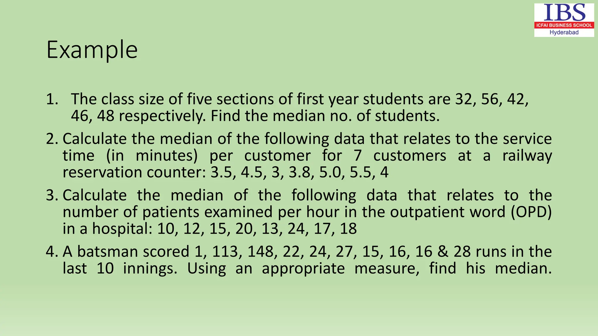
1. The class size of five sections of first year students are 32, 56, 42, 46, 48 respectively. Find the median no.
of students.
Key: Arrange the nos. in ascending order: 32, 42, 46, 48, 56
No. of observations n = 5 (odd)
Median value = [(n+1)/2]th observation
= [(5+1)/2]th observation
= 3rd observation = 46
The median no. of students is 46.
2. A batsman scored 1, 113, 148, 22, 24, 27, 15, 16, 16 & 28 runs in the last 10 innings. Using an appropriate
measure, find his average score.
Key: Since there are 2 extreme scores 113 & 148, hence mean would be affected by these values. Here,
median would be an appropriate measure.
Arrangement: 1, 15, 16, 16, 22, 24, 27, 28, 113, 148.
No. of observations, n = 10 (even)
Median = Mean of (n/2)th and (n/2+1)th observations
= Mean of 5th and 6th observations
= (22+24)/2 = 23
The median score of the batsman is 23 runs.

58. The Median – for grouped data
𝑀𝑒𝑑 = 𝑙 +
𝑛
2
− 𝑐𝑓
𝑓
× ℎ
• where
• l = lower class limit (or boundary) of the median class interval.
• c.f. = cumulative frequency of the class prior to the median class interval,
that is, the sum of all the class frequencies upto, but not including, the
median class interval
• f = frequency of the median class
• h = width of the median class interval
• n = total number of observations in the distribution.

59. The Median (grouped data) – Example 1

60. The Median (grouped data) – Example 2

61. The Median (grouped data) – Example 3
• A survey was conducted to determine the age (in years) of 120
automobiles. The result of such a survey is as follows:
Age of Auto No of Auto
0-4 13
4-8 29
8-12 48
12-16 22
16-20 8

62. Mode
• Mode is the value which occurs most frequently in a distribution.
• A distribution can have one or more than one modes.
• Mode is widely used while compiling the results of surveys. The options with maximum
frequencies are considered and decisions are taken accordingly.
• The demerits of arithmetic mean and median can be overcome with the help of mode.
• Mode can be calculated for grouped, ungrouped, discrete and continuous data.

63. Measures of Dispersion
• Let us consider the series of numbers:
5, 5, 5, 5, 5 (Mean = 5) 1, 3, 5, 7, 9 (Mean = 5) 1, 3, 4, 6, 11 (Mean = 5)
• Are the dataset same?
• Do they have the same characteristics?
• Does any difference exist among various observations of the datasets?
• Dispersion means spread or scatteredness of the various observations.
• Dispersion measures the extent to which the observations vary from
central value.
• Dispersion only measures the degree of variation, not the direction.

64. USEFUL MEASURES OF DISPERSION
• Range
• Interquartile Range
• Variance and Standard deviation

65. Range
• The range is the most simple measure of dispersion and is based on the location
of the largest and the smallest values in the data.
• Thus the range is defined to be the difference between the largest and lowest
observed values in a data set.
• Range (R) = Highest value of an observation – Lowest value of an observation
= H – L

66. • If the average of two distributions are almost same, then the distribution with
smaller range is said to have less dispersion.
• Lesser value of range indicates more consistency in the distribution.
• Coefficient of range = (L-S)/(L+S) [The relative measure of range]
• Range is widely used for statistical quality control. If the dimensions of products
are beyond a defined range, they are discarded.
• It facilitates the study of variations in the prices of shares, agricultural products
and other commodities.
• It also helps in weather forecasts by indicating minimum and maximum
temperature.
Range

67. Range – Example (Ungrouped Data)
• The following are the sales figures of a firm for the last 12 months
• Calculate the range of the given data.
Months 1 2 3 4 5 6 7 8 9 10 11 12
Sales (Rs
’000)
80 82 82 84 84 86 86 88 88 90 90 92

68. Interquartile Range or deviation
• The limitations or disadvantages of the range can partially be overcome by
using another measure of variation which measures the spread over the
middle half of the values in the data set so as to minimize the influence of
outliers (extreme values) in the calculation of range.
• Since a large number of values in the data set lie in the central part of the
frequency distribution, therefore it is necessary to study the Interquartile
Range (also called midspread).
• To compute this value, the entire data set is divided into four parts each of
which contains 25 per cent of the observed values. The quartiles are the
highest values in each of these four parts.

69. Interquartile Range or deviation
• The interquartile range is a measure of dispersion or spread of values in the
data set between the third quartile, Q3 and the first quartile, Q1.
• In other words, the interquartile range or deviation (IQR) is the range for the
middle 50 per cent of the data.
• Interquartile range (IQR) = Q3 – Q1
• Quartile deviation (QD) = (Q3 - Q1)/2, and
• Coefficient of QD = (Q3 - Q1)/(Q3 + Q1)

70. Interquartile Range
• The concept of IQR is shown in Fig.

71. Example
(i) Find the interquartile range of the given data
5, 8, 15, 26, 10, 18, 3, 12, 6, 14, 11
(ii) Find the interquartile range of the given data
11, 31, 21, 19, 8, 54, 35, 26, 29, 31, 35, 54

72. Example
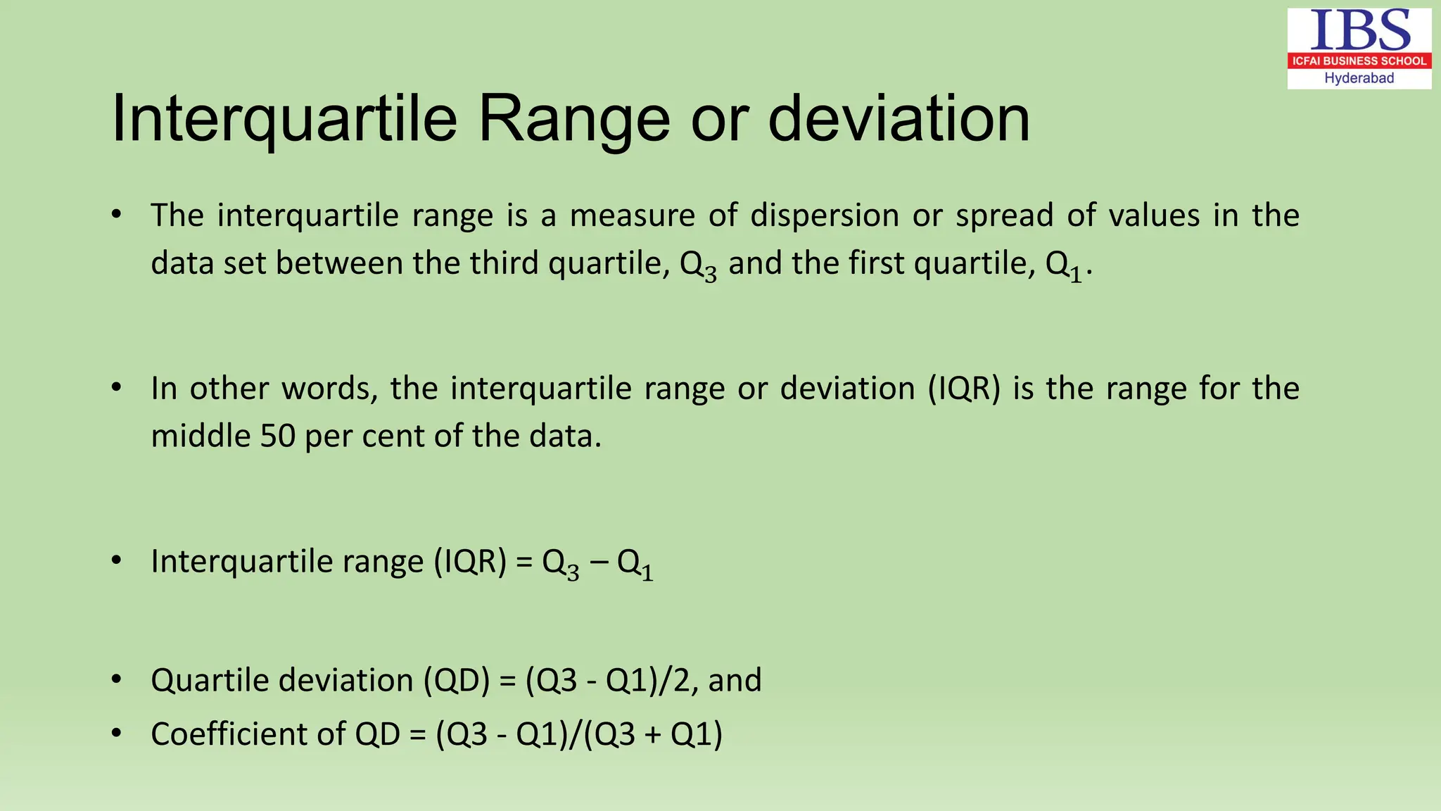
• Q1 = [(n+1)/4]th observation, and Q3 = [3(n+1)/4]th observation
• Ex: 1, 15, 16, 16, 22, 24, 27, 28, 113, 148; Q1 = 2.75th obs. and Q3 =
8.25th obs.
• Q1 = 2nd term + 0.75 (3rd term – 2nd term) = 15 + 0.75 (16-15) =
15.75
• Q3 = 8th term + 0.25 (9th term – 8th term) = 28 + 0.25
(113-28) = 49.25 QD = (49.25 – 15.75)/2 = 16.75
and
• Coeff. of QD = (49.25 – 15.75)/(49.25 + 15.75) = 0.5154 or
51.54%

73. Average Deviation Measures
• The mean absolute deviation of a dataset is the average distance
between each data point and the mean.
• It gives us an idea about the variability in a dataset.
• Here's how to calculate the mean absolute deviation.
• Step 1: Calculate the mean.
• Step 2: Calculate how far away each data point is from the mean using
positive distances. These are called absolute deviations.
• Step 3: Add those deviations together.
• Step 4: Divide the sum by the number of data points.

74. Example
1. The number of patients seen in the emergency ward of a hospital
for a sample of 5 days in the last month were 153, 147, 151, 156,
and 153. Determine the mean deviation and interpret.
2. Calculate the mean absolute deviation for a given data

75. Average Deviation Measures - Population Variance
and Standard deviation
Variance
• Every population has a variance, which is
symbolized by 𝜎2
(sigma squared).
• The formula for calculating the variance
is
• 𝜎2
=
𝑥−𝑥 2
𝑛
Standard Deviation
• The population standard deviation,
or 𝜎, is simply the square root of
the population variance.
• Because the variance is the
average of the squared distances
of the observations from the mean,
the standard deviation is the
square root of the average of the
squared distances of the
observations from the mean.
𝜎 = 𝜎2 =
𝑥 − 𝑥 2
𝑛
;
For
ungroup
data
𝑥 =
𝑥
𝑛
Population mean

76. Example
1. Calculate the variance and standard deviation for marks obtained for five students: 8, 4, 9, 11, 3

77. Example
x (x-𝑥) 𝑥 − 𝑥 2
Variance Std. Deviation Coeff. of Var.
8 8-7=1 1
Variance (𝜎2
)
= Σ 𝑥 − 𝑥 2
/n
= 46/5
= 9.2
Std Deviation (𝜎)
= Sqrt (Variance)
= Sqrt (9.2)
= 3.033
CV
= (𝜎/𝑥)*100
= (3.033/7)*100
= 43.33%
4 4-7=-3 9
9 9-7=2 4
11 11-7=4 16
3 3-7=-4 16
Σx=35
𝑥 = 7 Σ 𝑥 − 𝑥 2
= 46

78. Measures of Shape
• Skewness
• It is the degree of distortion from the symmetrical bell curve or the normal
distribution. It measures the lack of symmetry in data distribution.
• It differentiates extreme values in one versus the other tail. A symmetrical
distribution will have a skewness of 0.
• There are two types of Skewness: Positive and Negative

79. Measures of Shape
• Positive Skewness means when the tail on the right side of the distribution is
longer or flatter. The mean and median will be greater than the mode.
• Negative Skewness is when the tail of the left side of the distribution is longer
or flatter than the tail on the right side. The mean and median will be less than
the mode.
• So, when is the skewness too much?
• The rule of thumb seems to be:
•If the skewness is between -0.5 and 0.5, the data are fairly symmetrical.
• If the skewness is between -1 and -0.5(negatively skewed) or between 0.5
and 1(positively skewed), the data are moderately skewed.
• If the skewness is less than -1(negatively skewed) or greater than
1(positively skewed), the data are highly skewed.

80. Measures of Shape
• Kurtosis
• Kurtosis is all about the tails of the distribution —
not only the peakedness or flatness. It is used to
describe the extreme values in one versus the other
tail. It is actually the measure of outliers present in
the distribution.
• High kurtosis in a data set is an indicator that data
has heavy tails or outliers. If there is a high kurtosis,
then, we need to investigate why do we have so many
outliers.
• Low kurtosis in a data set is an indicator that data
has light tails or lack of outliers. If we get low
kurtosis(too good to be true), then also we need to
investigate and trim the dataset of unwanted results.

81. Measures of Shape
• Mesokurtic distribution: This distribution has kurtosis statistic similar to that of the
normal distribution. It means that the extreme values of the distribution are similar to
that of a normal distribution characteristic. This definition is used so that the standard
normal distribution has a kurtosis of three.
• Leptokurtic distribution (Kurtosis > 3): Distribution is longer, tails are fatter. Peak is
higher and sharper than Mesokurtic, which means that data are heavy-tailed or
profusion of outliers.
• Outliers stretch the horizontal axis of the histogram graph, which makes the bulk of the
data appear in a narrow (“skinny”) vertical range, thereby giving the “skinniness” of a
leptokurtic distribution.
• Platykurtic distribution (Kurtosis < 3): Distribution is shorter, tails are thinner than the
normal distribution. The peak is lower and broader than Mesokurtic, which means that
data are light-tailed or lack of outliers. The reason for this is because the extreme values
are less than that of the normal distribution.