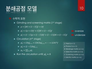
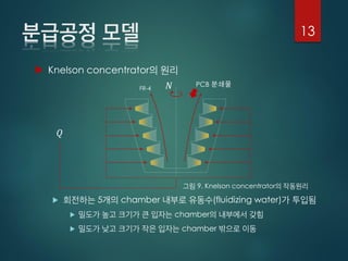
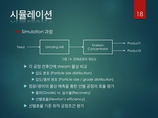
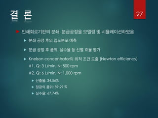
The document discusses modeling and simulation of printed circuit board (PCB) recycling processes including grinding and concentration using a Knelson concentrator. It describes:
1) Developing models for breakage, screening, and concentration using matrices to represent the processes.
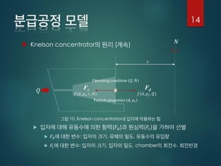
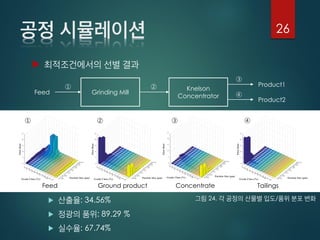
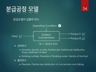
2) Simulating the effects of grinding mill and Knelson concentrator operating conditions like fluid flow rate and rotation speed on concentrate grade and recovery.
3) The models and simulations allow analyzing the recycling processes and optimizing operating conditions to maximize metal recovery from shredded PCBs.


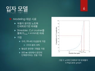
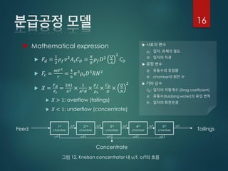


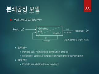
![ Particle
(Flowrate) FlowRate 1 x 1
( )
(Components) Componentsi 1 x 2
i ( ), text
ex> {‘Copper’, ‘FR-4’}
(Density) Densityi 1 x 2
i
ex> [2 9]
(Particle size range) PSRi 1 x 13
i (Nominal size)
ex> [45 62.5, 90, 125, … 2,800]
31](https://image.slidesharecdn.com/3fa5ca14-9811-409b-bed1-25df47fc1626-151021050604-lva1-app6892/85/150507-2015-31-320.jpg)
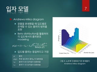
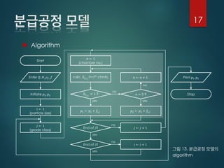
![ Particle ( )
(Particle size distribution) PSDi 1 x 13
i
ex> [0.1, 0.15, … 0.1]
(Grade distribution) GDi,j 13 x 12
i j
ex> [0 0.1 0.12, … 0.1]
(Drag coefficient) C_D 1 x 1
ex> 0.47
32](https://image.slidesharecdn.com/3fa5ca14-9811-409b-bed1-25df47fc1626-151021050604-lva1-app6892/85/150507-2015-32-320.jpg)


![[IJET-V1I5P5] Authors: T.Jalaja, M.Shailaja](https://cdn.slidesharecdn.com/ss_thumbnails/ijet-v1i5p5-151022010534-lva1-app6892-thumbnail.jpg?width=640&height=640&fit=bounds)

![[IJET-V1I4P9] Author :Su Hlaing Win](https://cdn.slidesharecdn.com/ss_thumbnails/ijet-v1i4p9-150824171458-lva1-app6891-thumbnail.jpg?width=640&height=640&fit=bounds)


