This document provides an overview of methods for solving inverse problems in mathematical physics. It discusses several types of inverse problems that arise for differential equations describing various physical phenomena. These include determining an unknown governing equation and its solution based on additional conditions. Inverse problems for elliptic, parabolic, hyperbolic, and kinetic equations are examined. Specific examples covered include inverse problems in potential theory, elasticity, heat transfer, fluid dynamics, and the Boltzmann equation. The document emphasizes that inverse problems are often ill-posed but can be addressed using regularization methods and incorporating additional structural information about the equations.


![Chapter 1
Inverse Problems for Equations
of Parabolic Type
1.1 Preliminaries
In this section we give the basic notations and notions and present also
a number of relevant topics from functional analysis and the general the-ory
of partial differential equations of parabolic type. For more detail we
recommend the well-known monograph by Ladyzhenskaya et al. (1968).
The symbol ~ is used for a bounded domain in the Euclidean space
R’~, x = (xl,...,x,~) denotes an arbitrary point in it. Let us denote
Q:~ a cylinder ftx (0, T) consisting of all points (x, t) ’~+1 with x Ef~
and t ~ (0,T).
Let us agree to assume that the symbol 0f~ is used for the boundary
of the domain ~ and ST denotes the lateral area of QT. More specifically,
ST is the set 0~ x [0, T] ~ R’~+1 consisting of all points (x, t) with z ~
and t G [0, T].
In a limited number of cases the boundary of the domain f~ is supposed
to have certain smoothness properties. As a rule, we confine our attention
to domains ~2 possessing piecewise-smooth boundaries with nonzero interior
angles whose closure (~ can be represented in the form (~ = tA~n=l~ for](https://image.slidesharecdn.com/0824719875inverse-141031173353-conversion-gate01/85/0824719875-inverse-22-320.jpg)
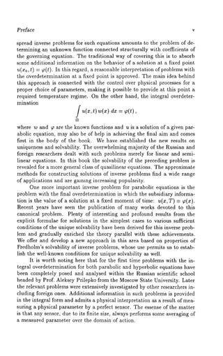
![4 1, Inverse Problems for Equations of Parabolic Type
usual, u~ and u~, respectively, instead of Dr u and D~ u. This should not
cause any confusion.
0
It is fairly commotno define the space Wl~(f~) as a subspace of W~( f~)
in which the set of all functions in f~ that are infinite differentiable and
have compact support is dense. The function u(x) has compact support in
a bounded domain f~ if u(x) is nonzero only in a bounded subdomain ~
of the domain ~ lying at a positive distance from the boundary of ~.
When working in HSlder’s spaces ch(~) and cl+h(~), we will as-sume
that the boundary of ~ is smooth. A function u(x) is said to satisfy
HSlder’s condition with exponent h, 0 < h < 1, and HSlder’s constant
H~(u) in ~ if
sup l u(x)--u(x’)l ~ H~(u) <
By definition, ch(~) is a Banach space, the elements of which are contin-uous
on ~ functions u having bounded
[u[~) : sup [u [+ H~(u).
In turn, c~+h(~), where l is a positive integer, can be treated as a Banach
space consisting of all differentiable functions with continuous derivatives
of the first l orders and a bounded norm of the form
I l u(~ +~~ ) = ~ ~ sup [D~ul+ ~ H~(D~u).
~=o ~=~ ~ ~=~
The functions depending on both the space and time variables with dis-similar
differential properties on x and t are much involved in solving non-stationary
problems of mathematical physics.
Furthermore, Lp, q(Qr), 1 ~ p, q < ~, is a Banach space consisting
all measurable functions u having bounded
][ u llp, q, Q~ = l u F d~ dt
0 ~
The Sobolev space W~’ ~ (Qr), p ~ 1, with positive integers I i ~ O,
i : 1, 2, is defined as a Banach space of all functions u belonging to the
sp~ce Lp(QT) along with their weak x-derivatives of the first l~ orders and
t-derivatives of the first l: orders. The norm on that space is defined by
P,QT :
k=O [~[=k k=l](https://image.slidesharecdn.com/0824719875inverse-141031173353-conversion-gate01/85/0824719875-inverse-25-320.jpg)
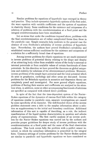
![1.1. Preliminaries
The symbol W~:~(Qr) is used for a subspace of W~"(Qr) in which
the set of all smooth functions in QT that vanish on ST is dense.
The space C2+~’1+~/2(QT), 0 < a < 1, is a Banach space of all
functions u in QT that are continuous on (~T and that possess smooth x-derivatives
up to and including the second order and t-derivatives of the
first order. In so doing, the functions themselves and their derivatives
depend continuously on x and t with exponents a and a/2, respectively.
The norm on that space is defined by
2
lu Q~ = ~ sup IDeal+sup ID,~I
sup I~D~u(x,t)-D~u(x’,t)l/lm-x’[
sup I Dtu(xt,) - Dtu(xt,’ ) I/It - t’
(x,t),(x,t~)EQw
+ ~’. sup I~D/~~u(x,t)-D~u(z,t’)l/It-t’l
÷ sup I Dtu(xt), - Dtu(xt’), I/I ~ - ~’ I~.
(x,t),(~,t’)eQT
In specific cases the function u depending on x and t will be treated as
an element of the space V~’°(Qr) comprising all the elements of W~’°(Qr)
that are continuous with respect to t in the L~(fl)-norm having finite
T u T~r= sup II~(,~)ll~,a+ll~ll~,~,
[o, T]
where u. = (u~,,..., u.~) and ~ =~u~ [~ . Th e meaning of the continuity
of the function u(-,t) with respect to t in the L~(fl)-norm is
°l 0 For later use, the symbol V~’ (@) will appear once we agree to con-sider
only those elements of V~’°(@) that vanish on ST.
In a number of problems a function depending on x and t can be
viewed as a function of the argument.t with values from a Banach space
over ~. For example, Le(O,T; W~(~)) is a set of all functions u(. ,t)
(0, T) with wlues in Wtp(a) and norm
T
0](https://image.slidesharecdn.com/0824719875inverse-141031173353-conversion-gate01/85/0824719875-inverse-26-320.jpg)
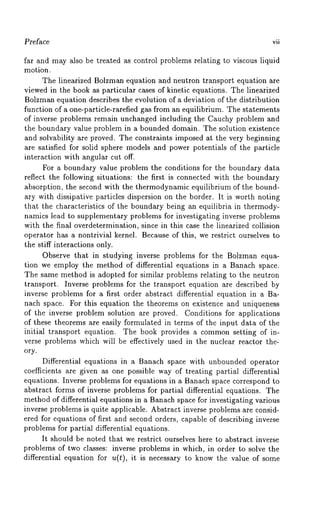
![6 1. Inverse Problems for Equations of Parabolic Type
Obviously, the spaces Lq(O, T; Lp(~)) and Lp, q(Qw) can be identified in a
natural way. In a similar line, the space
C([O, T]; W’p(fl))
comprises all continuous functions on [0, T] with values in W~(~).
obtain the Banach space C([O,T]; W~p(~)) if the norm on it is defined
, p,~ ¯
[0, 7]
We quote below some results concerning Sobolev’s embedding theory
and relevant inequalities which will be used in ~he sequel.
Recall tha~ the Polncare-~iedrichs inequality
ff u~(x) dx ~ c~(~)~ ~u~[~(x) dx
o
holds-true for all the functions u from W~(~), where ~ is a bounded domain
in the space R’~. The constant c1(~) depending only on the domain ~
b~o. unded by the value 4 (diamg)
Theorem 1.1.1 Let ~ be a bounded domain in the space Rn with the
pieccwise smooth boundary 0~ and let Sr be an intersection of ~ with any
r-dimensional hypersurface, r <_ n (in particular, if r = n then Sr =- ~,"
if r = n - 1 we agree to consider O~ as St). Then for any function
u 6 W~p(~), where l > 1 is a positive integer and p > 1, the following
assertions are valid:
(a) for n > pl and r > n-pl there exists a trace of u on ST belonging
to the space Lq(Sr) with any finite q < pr/(n-pl) and the estimate
is true."
(1.1.4) IlUllq,Sr <_cllu ~(~,~).
For q < pr/(n-pl) the operator embedding Wtp(~) into Lq(Sr) is
completely continuous;
(b) for n = pl the assertion of item (a) holds with any q < c~;
(c) for n < pl the function u is Hb’Ider’s continuous and belongs to the
class ck+h((~), where k : l - 1 - In/p] and h : 1 + [n/p] -
if niP is not integer and Vh < 1 if nip is integer. In that case the
estimate
(1.1.5) ]u (~+h) O)
b/P]d not , of](https://image.slidesharecdn.com/0824719875inverse-141031173353-conversion-gate01/85/0824719875-inverse-27-320.jpg)
![1.1. Preliminaries 9
Theorem 1.1.4 /the weak principle of maximum) Let the conditions
of Theorem 1.1.3 hold for the operator L and let a function u
satisfy the inequality Lu > 0 in f2 in a weak sense. Then
s+u.p u _< sup u
Corollary 1.1.1 Let the operator L be in line with the premises of Theorem
o
1.1.3 and let a function ~o ~ W~(Q) [1 W~(Q) comply with the conditions
~(x) > O a.e. in Q and ~(x) ~ const .
Then there exists a measurable set Q’ C f~ with
mes,~Q’> 0
such that L~ < 0 in
Proof On the contrary, let L~ > 0 in ~2. If so, the theorem yields either
~ < 0 in Q or ~o = const in fL But this contradicts the hypotheses of
Corollary 1.1.1 and proves the current corollary. ¯
Corollary 1.1.2 Let the operator L meet the requirements of Theorem
o
1.1.3 and let a function ~ 6 W~(QT) f] W~(Q) follow the conditions
~(x) > 0 a.e. in a and L~o(:~) co nst in a.
Then there exists a measurable set Q’ C Q with
mes~Q’ > 0
such that LW < 0 in
Proof Since LT ~ O, we have T ~ O, giving either T -- const > 0 or
T ~ const. If ~_-- const > O, then
=-
and the above assertion is simple to follow. For ~ ~ const applying Corol-lary
1.1.1 leads to the desired assertion. ¯](https://image.slidesharecdn.com/0824719875inverse-141031173353-conversion-gate01/85/0824719875-inverse-30-320.jpg)
![lO 1. Inverse Problems for Equations of Parabolic Type
For the purposes of the present chapter we refer to the parabolic
equation
(1.1.12) ut(x,t ) - (Lu)(x,t) = F(x,t), (x,t) QT= Qx (O,T ),
supplied by the initial and boundary conditions
(1.1.13) u(x,O) = a(x), x ¯ ~,
(1.1.14) u(x,t) = (z,t) ¯ ST --= 0Q × [0, T],
where the operator L is supposed to be uniformly elliptic. The meaning of
this property is that we should have
(i.1.15)
In what follows we impose for the coefficients of the operator L the following
constraints:
0
(1.1.16) Aij ¯ C((~), ~ Aq ¯ C((~), Bi ¯ L~o(a), C ¯
The direct problem for equation (1.1.12) consists of finding a solution
u of the governing equation subject to the initial condition (1.1.13) and the
boundary condition (1.1.14) when operating with the functions F and
the coefficients of the operator L and the domain ~ × (0, T).
Definition 1.1.1 A function u is said to be a solution of the direct problem
(1.1.12)-(1.1.14) from the class w2’l(I~2 ,,~., ~ if u ¯ 2W 1 2:o(Qr)a nd relations
(1.1.12)-(1.1.14) sati sfied almo st ever ywhere in t he corresponding do-mains.
Theorem 1.1.5 Let the coefficients ofthe operator L satisfy (1.1.15)-
o
(1.1.16) and let F ¯ L2(QT) and a ¯ W~(f~). Then the direct problem](https://image.slidesharecdn.com/0824719875inverse-141031173353-conversion-gate01/85/0824719875-inverse-31-320.jpg)
![1.1. Preliminaries
2,1 (1.1.12)-(1.1.14) has a solution u ¯ W~,o(Qr), this solution is unique
the indicated class of functions and the following estimate is valid:
(1.1.17) Ilull~)~, <c* Ilfll~,o~÷lla u,~ ,
where the constant c* does not depend on u.
In subsequent studies of inverse problems some propositions on solv-ability
of the direct problem (1.1.12)-(1.1.14) in the "energy" space
~l’°(Qr) will serve as a necessary background for important conclusions.
Definition 1.1.2 A function u is said to be a weak solution of the direct
°10 problem (1.1.12)-(1.1.14) from the c]ass ~’°(QT) ifu ¯ V~’ (QT) the
system (1.1.12)-(1.1.14) sat isfied in thesense of t he foll owing integral
identity:
t
0 ~ i,j=l
+ f u(x, t) ~(x, t)
- / a(x) (I)(x, dx
where (I) is an arbitrary
(x, ~)
The following result
t
0 ~
element of W~’l(Qr) such that O(x,t) = 0 for
is an excellent start in this direction.
Theorem 1.1.6 Let the coefficients of the operator L satisfy (1.1.15)-
(1.1.16) and let F ¯ L2,1(QT) and a ¯ L2(~). Then the direct problem
(1.1.11)-(1.1.14) has a weak solution u ¯ ~l~’° ~t~’)~ TZ~, this solution is unique
in the indicated class of functions and the energy balance equation is valid:
t , (1.1.19) ~ II~¯( ,t )ll2,~ ~ A,~ ~
0 ~ i,j=l](https://image.slidesharecdn.com/0824719875inverse-141031173353-conversion-gate01/85/0824719875-inverse-32-320.jpg)
![12 1. Inverse Problems for Equations of Parabolic Type
-£Biu~u-Cu 2) dzdv
i--1
t
=3 Ilall~,~ ÷ Fu dxdT,
0 ~
0<t<T.
Differential properties of a solution u ensured by Theorem 1.1.6 are
revealed in the following proposition.
Lemma1 .1.1 If all the conditions of Theorem 1.1.6 are put together with
F G L2(QT), then
o
u ¯ w2’lo(a x (¢,T)) C([¢,T], W~(f~)) 2,
for any e E (0, T).
For the further development we initiate the derivation of some esti-mates.
If you wish to explore this more deeply, you might find it helpful
01 first to establish the estimates for solutions u ¯ V2’°(Qr) of the system
(1.1.12). These are aimed to carry out careful analysis in the sequel.
Suppose that the conditions of Theorem 1.1.6 and Lemma 1.1.1 are
satisfied. With this in mind, we are going to show that any solution of
o1
(1.1.12)-(1.1.14) from V2’°(QT) admits for 0 < t < T the estimate
(1.1.20) tlu(. ,t)112,~ -< exp {-oct)H a I1~,
t
+ / exp{- oc( t - ~-))~ (,’ ’-1112~, d~-,
o
where oc=
(~) "’+~
/.z,= max{esssICup(¢a) 1es, ssu[pa i=1~ B f(*)]I/=}
and c~(Q) is the constant from the Poincare-Friedrichs inequality (1.1.3).
Observe that we imposed no restriction on the sign of the constant a.](https://image.slidesharecdn.com/0824719875inverse-141031173353-conversion-gate01/85/0824719875-inverse-33-320.jpg)
![1.1. Preliminaries 13
At the next stage, holding a number ¢ from the interval (0, T) fixed
and taking t = ¢, we appeal to identity (1.1.18). After subtracting the
resulting expression from (1.1.18) we get
(l.1.21)
t
where ¯ is an arbitrary element of W~’I(QT) that vanish on ST. Due to
the differential properties of the function u established in Lemm1a. 1.1 we
can rewrite (1.1.21) for 0 < e < t < T
t t
F~ dzdr.
It is important for us that the preceding relation occurs for any
¢ E W12’~(a x (¢,T)) vanishing on 0a x [¢,T].
o
Let r/(t) be an arbitrary function fi’om the space C°°([¢,T]). Obvi-ously,
the function q~ = u(x,t)r~(t) belongs to the class of all admissible
functions subject to relation (1.1.22). Upon substituting (I) u(z,t)rl(t)
into (1.1.22) we arrive
(1.1.23)
dr, 0<¢<t<T.](https://image.slidesharecdn.com/0824719875inverse-141031173353-conversion-gate01/85/0824719875-inverse-34-320.jpg)
![14 1. Inverse Problems for Equations of Parabolic Type
o
It is worth noting here that C~([¢, T]) is dense in the space L2([¢, T]). By
minor manipulations with relation (1.1.23) we are led
(1.1.24) -~ ~ Ilu(" , t) 112,
i,j:l u~ u~,
= Bi(X) ux, u ÷ C(x) ~ dx
+/ F(x,t) udx, O<¢<t<T.
By successively applying (1.1.2) and (1.1.15) to (1.1.24) we are
1 d
(1.1.25)
where
+#l[)u(’ , t )ll~,~+lIF(’,t)tI~,~’llu(’,t)ll~,~,
0<e<t<T,
#1 =max esssup Ic(x)l, esssup a~(x
The estimation of the first term on the right-hand side of (1.1.~5) can
done relying on Young’s inequality with p : q = 2 and ~ = u/#l, whose
use permits us to establish the relation
1 d ~ u
Applying the Poincare-~riedrichs inequality to the second term on the
right-hand side of (1.1.26) yields
d
(1.1.27)
0<e<¢<T,](https://image.slidesharecdn.com/0824719875inverse-141031173353-conversion-gate01/85/0824719875-inverse-35-320.jpg)
![1.1. Preliminaries
where
and c~(~) is the same constant as in (1.1.3).
Let us multiply both sides of (1.1.27) by exp {at} and integrate then
the resulting expression from e to t. Further passage to the limit as e --+ 0-4-
leads to the desired estimate (1.1.20).
The second estimate for u E v2T ~l(,0QT) in question follows directly
from (1.1.20):
(1.1.28)
sUP[o,t] ][u("r) ll2’a < c2(t) (]]a]]~,
O<t<T,
t
where
c~(t)= exp{ I a It}.
In the derivation of an alternative estimate we have to integrate rela-tion
(1.1.26) from e to t with respect to t and afterwards pass to the limit
as e -+ 0+. The outcome of this is
(1.1.29)
t
~ II~’,/,~-)ll~,da r_<~ II~’(,O)ll~,a
0
supII u(.,~ -)112,~
[o,t ]
-4- (#1 -4- ~t sup I1’~~( -) ~
2v] I[o,t
",
-4-s upII *4,~ )I1=,~
[o,t ]
t
x /II F(.,t)ll=,~ dr,
0
O<t<T.
Substituting estimate (1.1.28) into (1.1.29) yields that any weak solution](https://image.slidesharecdn.com/0824719875inverse-141031173353-conversion-gate01/85/0824719875-inverse-36-320.jpg)
![16 1. Inverse Problems for Equations of Parabolic Type
u e ~’°(QT) of the direct problem (1.1.12)-(1.1.14)satisfies the estimate
(1.1.30)
where
t t
0<t<T,
c3(t)=ul c2(t) [ l + 2tc2(t)(#l + ~-~ "
The next goal of our studies is to obtain the estimate of II u~(., t) 112,
for the solutions asserted by Theorem 1.1.6 in the case when t E (0, T].
Before giving further motivations, one thing is worth noting. As stated
in Lemma1 .1.1, under some additional restrictions on the input data any
solution u of the direct problem (1.1.12)-(1.1.14) from I}~’°(QT) belongs
the space W~:~(a x (¢, T)) for any ~ ¢ (0, T). This, in p~rticu[ar,
that the derivative ~,(. ,t) belongs to the space L~(~) for any t ~ (¢,T)
and is really continuous with respect to t in the L2(Q)-norm on the segment
Let t be an arbitrary number from the half-open interval (0, T]. Hold-ing
a number e from the interval (0, t) fixed we deduce that there exists
momentr * ~ [e, t], at which the following relation occurs:
t
(1.1.31) / < =
r* ¢ [<t], 0<e<t ~T.
In this line, it is necessary to recall identity (1.1.22). Since the set
admissible functions ¯ is dense in the space L~(QT), this identity should
be valid for any ¯ ~ L~(QT). Because of this fact, the equation
(1.1.32) ut(x,t) - (Lu)(x,t) = F(x,t)
is certainly true almost everywhere in Q ~ ~ x (~, t) and implies that
t t
r* ~2 r* ~2
0<c<t_<T,](https://image.slidesharecdn.com/0824719875inverse-141031173353-conversion-gate01/85/0824719875-inverse-37-320.jpg)
![1.1. Preliminaries
if v* and t were suitably chosen in conformity with (1.1.31).
readily see that (1.1.33) yields the inequality
i,j=l
Aij(x) u~(x,t) u~,(x,t)
t
r ° f~
i,j=l
Aij(x) %~(x, v*)%,(x, 7") dx
-t-2
t
t
17
One can
With the aid of Young’s inequality (1.1.1) the second term on the right-hand
side of (1.1.34) can be estimated as follows:
(1.1.35)
t
t 1 12 ~ 12)] dx
2(51u, 12+ 7 (lu~ d~-,
where
#1 --~ max esss upI c(x)I,
and (5 is an arbitrary positive number.
By merely setting (5 = 1/(4#1) we derive from (1.1.34)-(1.1.35)](https://image.slidesharecdn.com/0824719875inverse-141031173353-conversion-gate01/85/0824719875-inverse-38-320.jpg)
![18 1. Inverse Problems for Equations of Parabolic Type
useful inequality
(1.1.36) Ilux( ,t) ll~,~_< ~ Ilu~(.,~*)H =
t
+ - i i l ux dz dr
t
+ - dx dr,
/2
whose development is based on the Poincare-Friedrichs inequality (1.1.3)
and conditions (1.1.15). Having substituted (1.1.31) into (1.1.36) we
that
where
t t ][ux(’,t) ii~,r ~ _< c4(t)II [uxi2dxdr+i i1 F2dxdr
/2
0 ft 0 ~1
O<¢<t<_T,
c,(t) = /2#(t-O + 4#~ (1 + c1(~))
/2
and ~ is an arbitrary positive number from the interval (0, t).
The first term on the right-hand side of the preceding inequality can
be estimated on the basis of (1.1.30) as follows:
(1.1.37)
where
and
II ~(, t)117,-~< c ~(t)IaI I1~,+~ co(t)
t e (0, T],
~(t) = ~c~(t)c,(t)
c6(t ) = /2 -1 -[- 8t 2 C3(t ) C4(t)
In this context, it is necessary to say that estimates (1.1.20), (1.1.28),
o1
(1.1.30) and (1.1.30) hold for any solution u ~ V~’°(Qr) of the direct
lem (1.1.12)-(1.1.14) provided that the conditions of Theorem 1.1.6
Lemma 1.1.1 hold.
Differential properties of a solution u ensured by Theorem 1.1.5 are
established in the following assertion.](https://image.slidesharecdn.com/0824719875inverse-141031173353-conversion-gate01/85/0824719875-inverse-39-320.jpg)
![1.1. Preliminaries 19
Lemma 1.1.2 If, in addition to the premises of Theorem 1.1.5, Ft ~
L2(QT) and a E W~(12), then the solution u(x,t) belongs to C([O,T];
W~(~)), its derivative ut(x , t) belongs to
o
C([0, T], L2(~)) N C([e, T], W~(~)), 0 < ¢ < T.
o1
Moreover, ut gives in the space Vz’°(Qr) a solution of the direct problem
(1.1.38)
wt(x,t ) - (Lw)(x,t) = Ft(x,t)
w(x, O) = (La)(x) + F(x,
w(z, t) =
(x, t) E QT
XEST.
Roughly speaking, Lemma 1.1.2 describes the conditions under which
one can "differentiate" the system (1.1.12)-(1.1.14) with respect to
Let us consider the system (1.1.38) arguing as in the derivation
(1.1.20), (1.1.28), (1.1.30) and (1.1.37). All this enables us to deduce
in the context of Lemm1a .1.2 a solution u of the system (1.1.12)-(1.1.14)
has the estimates
(1.1.39)
(1.1.40)
(1.1.41)
t
, ~)I1~,d~r ~ c~(t)[ 11L+a r (. ,0)lt~,a
t 2
o
0<t<T,](https://image.slidesharecdn.com/0824719875inverse-141031173353-conversion-gate01/85/0824719875-inverse-40-320.jpg)
![1. i. Preliminaries
Note that we preassumed here that the function b(x,t) can be ex-tended
and defined almost everYwhere in the cylinder 0T. The boundary
condition (1.1.45) means that the boundary value of the function
u(x, t) - b(~,
is equal to zero on ST. Some differential properties of the boundary traces
of functions from the space W~’~"~(QT) are revealed in Ladyzhenskaya et
al. (1968).
Lemma 1.1.3 If u E W~’~"~(QT) and 2r+ s < 2m- 2/q, then
D7 Df u(.,0) E m- 2r - s - 2/ q(~).
Moreover, if 2r + s < 2m - l/q, then
"Wq~,~- 2r - s - i/q, -~ - r - s/2 - 1/(2q)(sT)
D[ D~ U]on
In wh~t follows we will show that certain conditions provide the solv-ability
of the direct problem (1.1.43)-(1.1.45) in the space V~’°(QT)
more detail see Ladyzhenskaya et al. (19~8)).
Theore1m.1 .’~T heree~ istsa solution~ , ~ V~( ¢) o~~ ro~le(m1. 1.43)-
(1.1.4~)~ ora ny~ ~ ~(~), b ~ W~’~(¢a)n d~ ~ ~,~(~),t ~is solution
is unique in the indicated class of functions and the stability estimate is
true:
sup 11 u( ¯ ,t) [[~,a + 11 ~ [[~,~T
[0, ~]
To decide for yourself whether solutions to parabolic equations are
positive, a first step is to check the following statement.
Theorem 1.1.8 (Ladyzhenskay~ et M. (1968) or Duvant and Lions (1972))
tel r E ~(~), a ~ ~(a), b ~ W~’I(~a) nd
the coefficient C(x) < 0 for x ~ ~ ;
a(x) >0 for x ~ ~;
b(~t,) >_ for (~,t ) ~ ;
F(~t, ) >_ for (~, t) E~ :r.
Then any solution u ~ V~’1 (0Qr) of problem (1.1.43)-(1.1.45) satisfies the
inequality u(x, t) >_ 0 almost everywhere in Q,T.](https://image.slidesharecdn.com/0824719875inverse-141031173353-conversion-gate01/85/0824719875-inverse-42-320.jpg)
![24 1. Inverse Problems for Equations of Parabolic Type
Using the results obtained in Ladyzhenskaya et al. (1968), Chapter 4,
conclude that there exists a unique solution v(k) 6 W2’ I(QT), q > n + 2, q
problem (1.1.50)-(1.1.52). Therefore, the function (k) and i ts d erivatives
v(k) satisfy H61der’s condition with respect to x and t in QT. This provides
support for the view, in particular, that v(~) is continuous and bounded
in QT and so the initial and boundary conditions can be understood in a
classical sense. The stability estimate (1.1.20) iml~lies that
(1.1.53) II(v- v(~))(.,t)ll2, < c*(Il a-a(~)II2,a + I IF- F(~ )II~,QT) ,
O<t<T.
We proceed to prove item (1). When a(x) ~ in ~, we mayassu me
without loss of generality that in ~
a(k) ~ 0
for any k 6 N. We have mentioned above that the function v(~) is contin-uous
and bounded in QT. Under these conditions Theorem 1.1.8 yields in
v(~)(x,t)> _
From Harnack’s inequality it follows that
v(~)(x,t)
for any t ~ (0,T], x ~ ft and k ~ N. We begin by placing problem
(1.1.50)-(1.1.52) with regard
w(x, t) : t) - v(k)(x,
It is interesting to learn whether w(x,t) > 0 in (~T and, therefore, the
sequence {v(~)}~=1 is monotonically nondecreasing. It is straightforward
to verify this as before. On the other hand, estimate (1.1.53) implies that
for any t ~ (0,T] there exists a subsequence {v(~p)}~=~ such that
as p --~ oo for almost all x 6 ft. Since {v(~)}~° is monotonically nonde- p:l
creasing, v(x, t) > 0 for almost all x 6 ~ and any t 6 (0, T].
We proceed to prove item (2). When a(x) ~ in ~ a ndF(x, t) ~ 0
in QT, we may assume that F(k) ~ 0 in QT for any k 6 N. Arguing as in
item (1) we find that (k) >0 inQT andby Harnack’s ineq uality dedu ce
that v(~)(x, T) > 0 for all x 6 ~. What is more, we establish with the
of (1.1.53) that v(x, T) > 0 almost everywhere in ft and thereby complete
the proof of Lemma 1.1.5. ¯](https://image.slidesharecdn.com/0824719875inverse-141031173353-conversion-gate01/85/0824719875-inverse-45-320.jpg)
![1.1. Preliminaries
Other ideas in solving nonlinear operator equations of the second kind
are connected with the Birkhoff-Tarsky fixed point principle. This
principle applies equally well to any operator equation in a partially ordered
space. Moreover, in what follows we will disregard metric and topological
characteristics of such spaces.
Let E be a partially ordered space in which any bounded from above
(below) subset D C E has a least upper bound sup D (greatest lower bound
inf D). Every such set D falls in the category of conditionally complete
lattices.
The set of all elements f E E such that a _< f _< b, where a and b
are certain fixed points of E, is called an order segment and is denoted
by [a,b]. An operator A: E H Eissaid to be isotonic if fl _< f2 with
fl, f2 ~ E implies that
AI~ <_ AI2.
The reader may refer to Birkhoff (1967), Lyusternik and Sobolev
(19S2).
Theorem 1.1.9 (Birkhoff-Tarsky) Let E be a conditionally complete lat-tice.
One assumes, in addition, that A is an isotonic operator carrying an
order segment [a, b] C E into itself. Then the operator A can have at least
one fixed point on the segment [a, b].
1.2 The linear inverse problem: recovering a source term
In this section we consider inverse problems of finding a source function
of the parabolic equation (1.1.12). We may attempt the function F in the
form
(1.2.1) F = f(x) h(x, t) + g(x,
where the functions h and g are given, while the unknown function f is
sought.
Being concerned with the operators L, /3, l, the functions h, g, a, b
and X, and the domain QT we now study in the cylinder QT =-- ~ x (0, T)
the inverse problem of finding a pair of the functions {u, f}, satisfying the
equation
(1.2.2) ut(x,t )- (Lu)(x,t)
= f(x) h(x,t)+g(x,t), (x,t)](https://image.slidesharecdn.com/0824719875inverse-141031173353-conversion-gate01/85/0824719875-inverse-46-320.jpg)
![26 1. Inverse Problems for Equations of Parabolic Type
the initial condition
(1.2.3.)( =, 0)
the boundary condition
(1.2.4) (Bu)(x,t) = b(z,t),
and the overdetermination condition
(x, t) ¯ sT= oa× [ 0, T],
(1.2.5) (lu)(x) = X(x), x ¯ f2.
Here the symbol L is used for a linear uniformly elliptic operator, whose
coefficients are independent of t for any x ¯ ~:
(1.2.6)
0
i,j=l
i=1
+ c(x) u(x,t),
- - i u, #_= const > 0.
i=1 i,j=l
The meaning of an operator B built into the boundary condition (1.2.4)
that
(1.2.7)
either (Bu)(x, -- u(x , t)
or (Bu)(x,t) =- aONu+ (x ~,tr)(x) u(x,t),
where
Ou _ ~ Aou.j(x,t) cos(n, Ox~)
ON - i,j=l
and n is the external normal to 0f2. Throughout the entire subsection,
we will assume that the function ~ is continuous on the boundary Of 2 and
~r>O.](https://image.slidesharecdn.com/0824719875inverse-141031173353-conversion-gate01/85/0824719875-inverse-47-320.jpg)
=0, (~, t)
and the overdetermination condition
(1.2.13) [l(u- v)](x) xEf~,
where Xl(x) = X(X) (l v)(x) and v is the unknown function to b e d ete r-mined
as a solution of the direct problem (1.2.9). This approach leads
the inverse problem of a suitable type.](https://image.slidesharecdn.com/0824719875inverse-141031173353-conversion-gate01/85/0824719875-inverse-48-320.jpg)
![1.2. The linear inverse problem: recovering a source term 29
By regarding an arbitrary function f from the space L2(fl) to be fixed and
substituting it into equation (1.2.14) we are now in a position on account
of Theorem 1.1.5 to find u ¯ W~2,,01~ T(g)) as a unique solution of the direct
problem (1.2.14)-(1.2.16). If this happens, Lemma1 .1.2 guarantees
the function u in question possesses the extra smoothness:
u(.,t) ¯ C([0,
and
ut(.,t ) ¯ C([0,T]; L2(~)).
In the light of these properties the intention is to use the linear operator
acting in accordance with the rule
T
1 / ut(z,t)w(t) dt z
(1.2.19) (A, f)(x) h, (x) ’ ’
0
where
T
h,(x) = h( x,t)w(t) dt
o
Of special interest is a linear operator equation of the second kind for
the function f over the space L2(~):
(1.2.20) f = A1 f + ¢,
where a known function ¢ belongs to the space L2(~).
In the sequel we will assume that the Dirichlet (direct) problem for
the elliptic operator
(1.2.21) (Lv)(x) = O,
has only a trivial solution unless the contrary is explicitly stated. Possible
examples of the results of this sort were cited in Theorem 1.1.3.
The following proposition provides proper guidelines for establishing
interconnections between the solvability of the inverse problem (1.2.14)-
(1.2.17) and the existence of a solution to equation (1.2.20) and vice versa.](https://image.slidesharecdn.com/0824719875inverse-141031173353-conversion-gate01/85/0824719875-inverse-50-320.jpg)
![30 1. Inverse Problems for Equations of Parabolic Type
Theorem 1.2.1 One assumes that the operator L satisfies conditions
(1.1.15)-(1.1.16), h, ht ¯ L~o(QT) and
T
0
for x ¯ ~ (5 =_ const), w ¯ L2(O,T) and
o ¯ w (a)
Let the Dirichlet problem (1.2.21) have a trivial solution only. If we agree
to consider
T
(1.2.22) ¢(z) ha(x) (L ~)(x), hi (x) -~ h(x , v)w (7") d’r
0
then the following assertions are valid:
(a) if the linear equation (1.2.20) is solvable, then so is the inverse
problem (1.2.14)-(1.2.17);
(b) if there exists a solution {u, f} of the inverse problem (1.2.14)-
(1.2.17), then the function f involved gives a solution to equation
(1.2.20)
Proof We proceed to prove item (a) accepting (1.2.22) to be true
equation (1.2.20) to have a solution, say f. If we substitute the function
into (1.2.14), then (1.2.14)-(1.2.16) can be solved as a direct problem.
account of Theorem 1.1.5 there exists a unique solution u ¯ W~:~(Qr) and
Lemma 1.1.1 gives
u(.,t) C([0, T] ; W~(~)
and
ut(.,t) ¯ C([O,T]; L2(f~))
The assertion will be proved if we succeed in showing that the function
u so constructed satisfies the supplementary overdetermination condition
(1.2.17). By merely setting
T
(1.2.23) / u(x,r)w(r) dv = ~1(~), x
0](https://image.slidesharecdn.com/0824719875inverse-141031173353-conversion-gate01/85/0824719875-inverse-51-320.jpg)
--0, xea, (~-~)(x)--0, xEO~,
having only a trivial solution by the assumption imposed at the very begin-ning.
Therefore, ~al = ~, almost everywhere in f~ and the inverse problem
(1.2.14)-(1.2.17) is solvable. Thus, item (a) is completely proved.
Let us examine item (b) assuming that there exists a pair of the
functions {u, f} solving the inverse problem (1.2.14)-(1.2.17). Relation
(1.2.14) implies that
T T
(1.2.27) f f
0 0
= f(x)h,(x),
where h~(x) = f? h(x,r)~(r)
With the aid of the overdetermination condition (1.2.17) and relation
(1.2.22) one can rewrite (1.2.27)
(1.2.28)
T f t)
0
dt + ~p(x) l(x) =f( x) hi (x)
Recalling the definition of the operator A1. (see (1.2.19)) we conclude
(1.2.28) implies that the function f is a solution to equation (1.2.20),
thereby completing the proof of the theorem. ¯](https://image.slidesharecdn.com/0824719875inverse-141031173353-conversion-gate01/85/0824719875-inverse-52-320.jpg)
![32 1. Inverse Problems for Equations of Parabolic Type
The following result states under what sufficient conditions one can
find a unique solution of the inverse problem at hand.
Theorem 1.2.2 Let the operator L comply with (1.1.15)-(1.1.16),
h, ht E L~(QT) and let
T j h(x,t)~(t)
o
dt >5>0 (5 _= const ),
0
w e L~([0, T]), ~ ~ W~(g~)fl W~(a). One assumes, in addition, that
the Dirichlet problem (1.2.21) has a trivial solution only and the inequality
holds."
(1.2.29) ml < 1,
m2(t) = exp {-at} esssup I h(x,
t
+ / exp {-a(t- r)} esssup~h,(.,v) l
J
o
,~ = m~x ~s~u~ [c(~)~, ~s~u~ ~:(~)
~
[i~1 ]1/2)
and c~(~) is the constant from the Poincare-Friedrichs inequality (1.1.3).
Then there exists a solution u ~ ~~,’ ~o(~), f e L~(~)o f th~ ~n~r~
lem (1.2.14)-(1.2.17), this solution is unique in the indicated class of func-tions
and the following estimates are valid with constant c* from (1.1.17):
(1.2.30) IIf II~a,< _1 - ml
-c1* 5
(1.2.31) 11 u ]l~)~ _~
1 - T/-/1
T
× o ess~up I h(x, t)12 dr)](https://image.slidesharecdn.com/0824719875inverse-141031173353-conversion-gate01/85/0824719875-inverse-53-320.jpg)
![1.2. The linear inverse problem: recovering a source term 35
Le(f~) and substituting it into equation (1.2.34). According to Theorem
1.1.5 there exists a unique solution u ¯ W~’ltr) ~ of the direct problem
(1.2.34)-(1.2.36) with the extra smoothness property:
u(. ,t) ¯ C([0,T];
and
ut(.,t ) ¯ C([0, T]; L;(f~))
For further analysis we refer to the linear operator
A2: L~(f~) ~ L2(fl)
acting in accordance with the rule
1
(1.2.39) (A2f)(z) h( x,T) ut (x’T)’
and the linear operator equation of the second kind for the function f over
the space L2(ft):
(1.2.40) f = A~ f + ¢,
where a known function ¢ belongs to the space L~(f~).
Theorem 1.2.3 Let the operator L satisfy conditions (1.1.15)-(1.1.16) and
lath, ht ¯ Loo(QT), [h(x,T)[ >_ 6 > O forx ¯ ~ (6 const), ¢ ¯
o
W~(fl) I3 W~(ft). Assuming that the Dirichlet problem (1.2.21) can have a
trivial solution only, set
1
(1.2.41) ¢(~)- h(x,T) (L~)(~:).
Then the following assertions are valid:
(a) /f the linear equation (1.2.40) is solvable, then so is the inverse
problem (1.2.34)-(1.2.37);
(b) if there exists a solution {u, f} of the inverse problem (1.2.34)-
(1.2.37), then the function f involved gives a solution to the linear
equation (1.2.40).
Theorem 1.2.3 can be proved in the same manner as we carry out the
proof of Theorem 1.2.1 of the present chapter or that of Theorem 4.2.1
from Chapter 4.](https://image.slidesharecdn.com/0824719875inverse-141031173353-conversion-gate01/85/0824719875-inverse-56-320.jpg)
![36 1. Inverse Problems for Equations of Parabolic Type
So, the question of the inverse problem solvability is closely connected
with careful analysis of equation (1.2.40) of the second kind. By exactly
the same reasoning as in the case of inequality (1.2.32) we deduce that the
operator A2 admits the estimate
(1.2.42) NA~fN2,~~ m3Nf[I2,~, f E L2(f~),
where
rn3=~I ,{ex{p- c~T }e ssnsu]p h (x,0 )I
T
+S e xp{- °<(:r~- ’))e sssIutdp"’ t ) I dr}
0
~= 2c,(a) ~’ +~’ ’
=max esssup Ic(~)l, esssup[£ ~ ~ i=1
and c, (f~) is the constant from the Poincare-Friedrichs inequality (1.1.3).
After that, applying estimate (1.2.42) and the fixed point principle
the linear operator A~ with the subsequent reference to Theorem 1.2.3 we
obtain an important result.
Theorem 1.2.4 Let the operator L satisfy conditions (1.1.15)-(1.1.16) and
let h, ht ~ Loo(QT), Ih(x,T) l >_ 5 > 0 for x ~ ~ (~ const) and
0 ~ ¯ w~(ar)~ w~,(a).
One assumes, in addition, that the Dirichle~ problem (1.2.21) has a trivial
solution only. If the inequality
(1.2.43) m3 < 1
is valid with constant m3 arising from (1.2.42), then there exists a solu-tion
u ~ W~,’01(QT), f ~ L~(~) of the inverse problem (1.2.34)-(1.2.37),](https://image.slidesharecdn.com/0824719875inverse-141031173353-conversion-gate01/85/0824719875-inverse-57-320.jpg)
![1.2. The linear inverse problem: recovering a source term 37
this solution is unique in the indicated class of functions and the following
estimates
(1.2.44) Ilfll~,~ ~ l_m~--~ll5~ll~,~,
-C*I~
(1.2.45) Ilull~)T _< l_rn---~[[L~[[2,
T 1/2
are valid with constant c* from (1.1.17).
Theorem 1.2.4 can be proved in a similar way as we did in the proof
of Theorem 1.2.2.
We now present some remarks and examples illustrating the results
obtained.
Remark 1.2.1 In dealing with the Laplace operator
(Lu)(x--, zX(~x, t)= _
we assume that the function h depending only on t satisfies the conditions
h, h’ e C[0,T] ~(t), ~’(t) _> 0, ~(T)
Plain calculations give
1
c~- 2c,(~2) and rna = 1-rha,
where
T
0
exp {-c~ (T - t)} dr.
Since rna > 0, the inequality gna < 1 holds true. On the other hand, rha > 0
for an arbitrary function h(t) > 0 with h(T) ¢ 0. Therefore, 0 < rna < 1
for any T > 0 and, in that case, Theorem 1.2.4 turns out to be of global
character and asserts the unique solvability for any T, 0 < T < oo.](https://image.slidesharecdn.com/0824719875inverse-141031173353-conversion-gate01/85/0824719875-inverse-58-320.jpg)
![1. Inverse Problems for Equations of Parabolic Type
Example 1.2.1 Let us show how one can adapt the Fourier method
of separation of variables in solving inverse problems with the final
overdetermination. With this aim, we now turn to the inverse problem of
recovering the functions u(x) and f(z) from the set of relations
(1.2.46) ut(x ,t) = uzx(x,t) + f(x) 0 < x < 7r ,
(1.2.47) u(x,O) = 0 < x < 7r,
(1.2.48) u(O,t) = uOr, ) =O, 0 < t < T,
(1.2.49) u(x, T) = ~(x), 0 < x < 7r,
O<t<T,
keeping ~ E W~(0, 1) with the boundary values
9(0) = =
It is worth noting here that in complete agreement with Remark 1.2.1 the
inverse problem at hand has a unique solution for any T, 0 < T < cx~.
Following the standard scheme of separating variables with respect to the
system (1.2.46)-(1.2.48) we arrive
(1.2.50)
t
u(x,t) = E / fk exp {-k2(t - ~-)} dr sin/ca
k=l 0
= E f~ k-~ [1 - exp {-k~t)] sinkx,
k=l
where
2 ] f(x) sinkx dx.
0
The system {X~(x) si n kx }~°=l and th e se quence {~ k : k 2) k¢=l¢ are
found as the eigenfunctions and the eigenvalues of the Sturm-Liouville
operator associated with the spectral problem
(1.2.51) X~(x) + )~ X(x) = O, 0 < x < ~r, Xa(O) = X~(~r)
Being a basis for the space L2(0, 7r), the system {sin kx}~=l is orthogonal
and complete in it. In this view, it is reasonable to look for the Fourier
coefficients f~ of the unknown function f with respect to the system](https://image.slidesharecdn.com/0824719875inverse-141031173353-conversion-gate01/85/0824719875-inverse-59-320.jpg)
![42 1. Inverse Problems for Equations of Parabolic Type
by (1.2.39) comes first. This type of situation is covered by the following
assertion.
Theorem 1.3.1 Let the operator L satisfy conditions (1.1.15)-(1.1.16) and
let h, h~ ¯ L~o(QT), [h(x,T)[ >_ 6 > 0 forx ¯ (~ (6 const). Then the
operator A2 is completely continuous on L2(ft).
Proof First of all we describe one feature of the operator A2 emerging from
Lemma1s .1.1 and 1.1.2. As usual, this amounts to considering an arbitrary
function f from the space L2(12) to be fixed and substituting it into (1.2.34).
Such a trick permits us to demonstrate that the system (1.2.34)-(1.2.36)
is of the same type as the system (1.1.12)-(1.1.14). When solving problem
(1.2.34)-(1.2.36) in the framework of Theorem 1.1.5 one finds in passing
unique function u ¯ W22~,01 (Qr) corresponding to the function having been
fixed above. Lemma1 .1.2 implies that
o
u, ¯ C([O,T];L2(~))NC([~,T];W~(f~)), 0<~<T.
Therefore, the operator A2 specified by (1.2.39) acts, in fact, from L~(f~)
o
into W~(~).
In the estimation of A~(f) in the W~(f~)-norm we make use of in-equality
(1.1.42) taking in terms of the system (1.2.34)-(1.2.36) the
(1.3.1) II ut~(.,T) I}~,n _~ cs(T) [[[/h(.,0)[[~,n
T
0
where c5 and c~ are the same as in (1.1.42) and do not depend on
Combination of relations (1.2.39) and (1.3.1) gives the estimate
(1.3.2)
where
C7 ~
T
Note that estimate (1.3.2) is valid for any function f from the space L2(~)
and the constant c~ is independent of f.](https://image.slidesharecdn.com/0824719875inverse-141031173353-conversion-gate01/85/0824719875-inverse-63-320.jpg)
![44 1. Inverse Problems for Equations of Parabolic Type
Proof We proceed to prove item (a). Let (1.3.3) have a trivial solution
only. By Corollary 1.3.1 there exists a solution to the nonhomogeneous
equation (1.2.40) for any ¢ L2(Q) (and, in particular, for ¢ of the f orm
(1.2.41)) and this solution is unique. The existence of the inverse problem
(1.2.34)-(1.2.37) solution follows now from Theorem 1.2.3 and it remains
to show only its uniqueness. Assume to the contrary that there were two
distinct solutions {ul, fl} and {u2, f2) of the inverse problem (1.2.34)-
(1.2.37). It is clear that fl cannot be equal to f2, since their coincidence
would immediately imply the equality between ul and u~ by the uniqueness
theorem for the direct problem of the type (1.2.34)-(1.2.36). According
item (b) of Theorem 1.2.3 the function fl - f2 is just a nontrivial solution
to the homogeneous equation (1.3.3). But this disagrees with the initial
assumption. Thus, item (a) is completely proved.
We proceed to examine item (b). Let the uniqueness theorem hold
for the the inverse problem (1.2.34)-(1.2.37). This means that the homo-geneous
inverse problem
(1.3.4) ut(x, t) - (Lu)(x, t) = f(x) (x, t) ¯ QT,
(1.3.5) u(x,O) = x
(1.3.6) u(x,t) = 0, (x,t) ¯ ST,
(1.3.7) u(x,T) = x ¯
might have a trivial solution only. Obviously, the homogeneous equation
(1.3.3) is associated with the inverse problem (1.3.4)-(1.3.7) in the
work of Theorem 1.2.3.
Let us show that (1.3.3) can have a trivial solution only. On the
contrary, let f ¯ L2(~) be a nontrivial solution to (1.3.3). Substituting
f into (1.3.4) and solving the direct problem (1.3.4)-(1.3.6) by appeal
Theorem 1.1.5, we can recover a function u ¯ W~:01(Qr) with the extra
smoothness property indicated in Lemma 1.1.2. It is straightforward to
verify that the function u satisfies also the overdetermination condition
(1.3.7) by a simple observation that equation (1.3.4) implies
ut(x, T) - (Lu)(x, T) -= f(x) T), ( x, t ) ¯
On the other hand, the function f is subject to relation (1.3.3), that is,
h(x,T)(A2 f)(z) = f(x) h(x,T),
From definition (1.2.39) of the operator A2, two preceding relations
combination with the boundary condition (1.3.6) it follows that the function
u(x, T) solves the Dirichlet problem
L[u(x,T)] =0, x¯f~; u(x,T)=O, x¯~;](https://image.slidesharecdn.com/0824719875inverse-141031173353-conversion-gate01/85/0824719875-inverse-65-320.jpg)
![46 1. Inverse Problems for Equations of Parabolic Type
and consider the related linear equation of the second kind
(1.3.14) f= .~f÷3, where ~(x)-
h(x, T) [(L~)(x) + A~(x)]
For the inverse problem (1.3.9)-(1.3.12) and equation (1.3.14)
possible to obtain a similar result as in Theorem 1.2.3 without the need for
the triviality of the unique solution of the corresponding stationary direct
problem (1.3.8). The well-founded choice of the parameter A assures
of the validity of this property. By analogy with Theorem 1.3.1 the linear
operator ~2 turns out to be compact. By exactly the same reasoning as in
Theorem 1.3.2 we introduce a preliminary lemma.
Lemma1 .3.1 Let the operator L satisfy conditions (1.1.15)-(1.1.16) and
lel h, h~ E L~(QT), I h(x,T) I >_ 5 > 0 for x ~ (~ (5 =_ const) and
o e
Then the following assertions are valid:
(a) if Ihe linear equalion f = ~2 f has a lrivial solution only, ihere
exists a solution of Zhe inverse problem (1.3.9)-(1.3.12) and this
solution is unique in Zhe indicated class of functions;
(b) ff the uniqueness theorem holds for lhe inverse problem (1.3.9)-
(1.3.12), there exis¢s a solution of ¢he inverse problem (1.3.9)-
(1.3.12) and Zhis soluZion is unique in ihe indicated class of func-tions.
It is worth emph~izing once again that the inverse problems (1.2.34)-
. ~
(1.2.37) and (1.3.9)-(1.3.12) are eqmvalent to each other from the
point of existence and uniqueness. With this equivalence in view, Lemma
1.3.1 permits us to prove the assertion of Theorem 1.3.2 once we get rid
of the triviality of the inverse problem (1.2.21) solution after the appro-priate
"shift" of the spectrum of the operator L. This profound result is
formulated below as an alternative.
Theorem 1.3.3 Let the operator L satisfy conditions (1.1.15)-(1.1.16) and
let h, ht ~ L~(QT), ]h(x,T) ] >_ 5 > 0 for x ~ ~ (5 const ) and
o w (a)
Then the following alternative is true: either a solution of the inverse prob-lem
(1.2.34)-(1.2.37) exists and is unique or the homogeneouisn verse prob-lem
(1.3.4)-(1.3.7) has a nontrivial solution.
In other words, this assertion says that under a certain smoothness
of input data (see Theorem 1.3.3) of the inverse problem with the final
overdetermination the uniqueness theorem implies the existence one.](https://image.slidesharecdn.com/0824719875inverse-141031173353-conversion-gate01/85/0824719875-inverse-67-320.jpg)
![1. Inverse Problems for Equations of Parabolic Type
along with
u, e C([0,T];
(ui)t C([0,T];
52
In complete agreement with Lemma1 .1.2 the functions
vi(x,t ) -- (ui)t(x,t), i = 1, 2,
belong to ~/~’°(QT) and the following relations
(1.3.31) (vi)t(x,t) - (Lvi)(x,t) = f±(x)ht(x,t),
(1.3.32) vi(x, O)
(1.3.33) vi(x,t ) = O, (x,t)
are valid in the sense of the corresponding integral identity.
Before we undertake the proof with the aid of Lemma 1.1.5, let us
observe that the functions f±h(x, 0) and f±ht(x,t) can never be identi-cally
equal to zero once at a time. Indeed, assume to the contrary that
f±h(x,O) -- 0 and f±ht(x,t ) =_ 0 simultaneously. Then the Newton-
Leibniz formula gives
T
f+ (x) h(x, T) = f± (x) h(x, O) ÷ f t (x, t ) d
o
yielding
f± (x) h(x, = 0
over f~. However, by requirement,
f+
and
f-S0.
This provides support for the view that h(x, T) _-- 0, x ¯ ~, which disagrees
with h(x, T) >
In accordance with what has been said, Lemma 1.1.5 is needed to
derive the inequality
(1.3.34) (ui)t(x,T) =_ vi(x,T ) > O, x ¯ ~, i = 1, 2.
On the other hand, Lemma 1.1.2 implies that](https://image.slidesharecdn.com/0824719875inverse-141031173353-conversion-gate01/85/0824719875-inverse-73-320.jpg)
![1.3. The linear inverse problem: the Fredholm solvability 53
Having stipulated these conditions, equation (1.3.21) leads to the relations
(1.3.35) (ui)t(x,T) - (L#)(x) f+(x) h( x,T), x Ef t, i = 1, 2.
Here we used Mso that the values of ul and u2 coincide at the moment
t = T and were denoted by #.
When L# ~ 0 in ft, it follows from (1.3.30) and Corollary 1.1.2 that
there exists a measurable set ~’ C f~ such that
mesn ~’ > 0
and
(1.3.36) (n#)(m) < O, x e
By assumption, h(x,T) > 0. In view of this, relations (1.3.35)-(1.3.36)
imply that f+(x) > 0 and f-(x) > 0 in fY. But this contradicts
ft the identity f+ . f- = 0, valid for the functions f+ and f- of such
constructions.
For the case L# -= 0 relation (1.3.35) can be rewritten
(1.3.37) (ui)t(x,T) f+(x) h( x,T), x ~f t, i 1, 2.
Therefore, relations (1.3.34) and (1.3.37) imply that again f+ > 0
f- > 0 in ~. As stated above, this disagrees with constructions of the
functions f+ and f-. Thus, all possible cases have been exhausted and the
theorem is completely proved. ¯
Remark 1.3.2 A similar uniqueness theorem is still valid for the inverse
problem of recovering the source term coefficient in the general statement
(1.2.2)-(1.2.5) (see Prilepko and Kostin (1992a)).
Theorems 1.3.3 and 1.3.6 imply immediately the unique solvability of
the inverse problem (1.2.34)-(1.2.37). We quote this result for the inverse
problem (1.2.2)-(1.2.5) in a commonse tting.
Theorem 1.3.7 Let the operator L satisfy conditions (1.1.15)-(1.1.16) and
the coefficient C(m) >_ 0 for x E f~. One assumes, in addition, lhat
ht~ Loo(QT), ~ e C(Oft), = O,a =_ O, b =_ O, w ~L2([ 0,T]), X G W~(~
and (/3X)(0e) form~ 0~. Also, let h( m,t) >_ 0 and ht( ) >_0 almost
everywhere in QT; or(x) >_ 0 for m ~ Oft; w(t) > 0 almost everywhere on
(0, T) and [l(h)](x) >_ 5 > 0 for x ~ ~ const ). Then t he in verse prob-lem
has a solution e f C2(ft), this solution
is unique in the indicated class of functions and the estimate
(~)
is true, where the constant c is expressed only in terms of the input data
and does not depend on u and f.](https://image.slidesharecdn.com/0824719875inverse-141031173353-conversion-gate01/85/0824719875-inverse-74-320.jpg)
![56 1. Inverse Problems for Equations of Parabolic Type
In this regard, the question of the solution existence for the nonlinear
inverse problem (1.4.1)-(1.4.4) arises naturally. We begin by deriving
operator equation of the second kind for the coefficient f keeping
(1.4.10)
gT, b, gt E Wp2’a(Q
~(x)_>6>0 in
, p_>n+l; L~6E;
b(x,O):O for x
By relating a function f from E to be fixed we substitute it into equation
(1.4.1). The well-known results of Ladyzhenskaya and Uraltseva (1968)
guide the proper choice of the function u as a unique solution of the direct
problem (1.4.1)-(1.4.3). It will be convenient to refer to the nonlinear
operator
A: E~-*E
with the values
1
(1.4.11) (Af)(x) ,[ut(x,T)-(L~)(x)-g(x,T)]
and consider over E the operator equation of the second kind associated
with the function f:
(1.4.12) f = At.
We will prove that the solvability of equation (1.4.12) implies that of the
inverse problem (1.4.1)-(1.4.4).
Lemma1 .4.1 Let the operator L satisfy conditions (1.1.15)-(1.1.16), the
coefficient C(x) <_ 0 for x ~ f~ and condition (1.4.10) hold. Also, let the
compatibility condition
b(x, T) = ~(~)
be fulfilled for x ~ Of L One assumes, in addition, that equation (1.4.12)
admits a solution lying within E_. Then there exists a solution of the
inverse problem (1.4.1)-(1.4.4).
Proof By assumption, equation (1.4.12) has a solution lying within E_,
say f. Substitution f into (1.4.1) helps find u as a solution of the direct
problem (1.4.1)-(1.4.3) for which there is no difficulty to establish
ut ~ Wv l(Qr) , ut(.,T) ~ and (Lu)(. T) (se e Ladyzhenskaya and
Uraltseva (1968)). We will show that the function u so defined satisfies
also the overdetermination condition (1.4.4). In preparation for this, set
= x e a.](https://image.slidesharecdn.com/0824719875inverse-141031173353-conversion-gate01/85/0824719875-inverse-77-320.jpg)
+ f(x)(9~-~l)=O,
Combination of the boundary condition (1.4.3) and the compatibility con-dition
gives
(1.4.16) (9 - ~l)(x) = 0, x e cOf~.
As C(z) _~ 0 in ~ and f E E_, the stationary direct problem (1.4.15)-
(1.4.16) has only a trivial solution due to Theorem 1.1.3. Therefore, the
function u satisfies the final overdetermination condition (1.4.4) and the
inverse problem (1.4.1)-(1.4.4) is solvable, thereby completing the proof
the lemma. ¯
As we have already mentioned, the Birkhoff-Tarsky theorem is much
applicable in solving nonlinear operator equations. A key role in developing
this approach is to check whether the operator A is isotonic.
Lemma1 .4.2 Let the operator L satisfy conditions (1.1.15)-(1.1.16), the
coeJ:ficient C(x) <_ 0 in ~, conditions (1.4.10) hold, g(x, t) >_ 0 and gt(x, >_
0 in QT. If, in addition, the compatibility conditions
b(x,T) =- ~(x) and ,0) = g( x, O)
are fulfilled for any x ~ 0~, then A is an isotonic operator on E_.
Proof First of all we stress that E_ is a conditionally complete lattice.
Let fl and f2 be arbitrary elements of E_ with fl _< f2. One trick we
have encountered is to substitute fl and f2 both into equation (1.4.1) with
further passage to the corresponding direct problems for i = 1, 2:
(1.4.17) u~(z, t) - ( Lu’) (x,
= f~(x)ui(x,t)+g(x,t), (x,t)~QT,
(1.4.18) u’(x, O)
(1.4.19) ui(x,t) = b(x,t), (x,t)](https://image.slidesharecdn.com/0824719875inverse-141031173353-conversion-gate01/85/0824719875-inverse-78-320.jpg)
![5s 1. Inverse Problems for Equations of Parabolic Type
In this regard, the conditions of the lemma assure that the function wi -- ut
presents a solution of the direct problem
(1.4.2o) w~(tx), - (L~o~)(x,
= f~(x) wi(x,t)+gt(x,t), (x,t)¯QT,
(1.4.21) w~(x,O) = g(x,O), x ¯ ~,
(1.4.22) wi(x,t) = b~(x,t), (x,t) ¯ ST.
Being solutions of (1.4.17)-(1.4.19), the functions v 2 - u 1 andh =
f2 - fl are subject to the set of relations:
(1.4.23) vt(x,t) - (Lv)(x,t) -f~(x)v(x,t)
= h(x)ul(~,t), (~,t) ¯ Q~,
(1.4.24) v(x,O=) O, x ¯
(1.4.25) v(x,t) = (x,t)
Just now it is necessary to keep in mind that fl < f2. On ~ccount of
Theorem1 .1.8 and Lemma1 .1.5 the systems (2.4.17)-(2.4.19) and (2.4.20)-
(2.4.22) provide that h(x) u~(x,t) > 0 and h(x) u~(x,t) >_ for (x,t) ¯ QT
Once again, appealing to Theorem 1.1.8 and Lemma 1.1.5, we deduce that
vt(x,T ) > 0 in f2. By definition (1.4.11) of the operator A, Af~ < Aft,
what means that A is isotonic on E_. This proves the assertion of the
lemma. ¯
We now turn to a common setting and proving the principal global
result concerning the unique solvability of the inverse problem at hand.
Theorem 1.4.2 Let the operator L satisfy conditions (1.1.15)-(1.1.16) and
the coefficient C(x) < 0 in f2. Let g, b, t ¯W~’~(Qr), p > n+l; g(x,t) >
and gt(x,t ) >_ 0 for (x,t) ¯ QT; L~ ¯ E; ~(x) >_ ~ > 0 in f2 -- const).
Also, we lake for granted the compatibility conditions
~(~o, )= o ,
b(x,7"):99(x) and b,(x,O)=g(x,O) for
and require that
(1.4.26)
L[~°(xT, ) ~(~)] _<o, x ¯~,
where u° refers to a solution of problem (1.4.1)-(1.4.3) with f --- O. Then
the inverse problem (1.4.1)-(1.4.4) has a solution u ¯ W~p,~(Q~f) ,
and this solution is unique in the indicated class of functions.](https://image.slidesharecdn.com/0824719875inverse-141031173353-conversion-gate01/85/0824719875-inverse-79-320.jpg)
![.4. The nonlinear coe~cient inverse problem 59
Proof First we are going to show that on E_ there exists an order segment
which is mapped by the operator A onto itself. Indeed, it follows from the
foregoing that (1.4.26) implies the inequality
1 L[uO(x,T)_~(x) ] <0 ce~
(1.4.27) A(0) -= - ’ ’
and, consequently,
A: E_ ~-~ E_.
Let us take a constant M from the bound
1
(1.4.28) M >_ P-~ [(L~)(x) g( x, T)], x e f~.
By definition (1.4.10) of the operator
1
(1.4.29) A(-M)=- ~(x) [ut(x’T)-(L~)(x)-g(x’T)]’
where u is a solution of the system (1.4.1)-(1.4.3) with constant -M stand-ing
in place of the coefficient f.
Before giving further motivations, let us recall that the coefficients of
the operator L do not depend on t. For the same reason as before, the
function ut gives a solution from ~’°(Qr) of the direct problem
wt - Lw = -Mw + gt , (x, t) QT,
w(x0, ) = 9(x, x e n,
¯ w(x,t)= b,(x,t), sT,
whence by Theorem 1.1.8 and Lemma1 .1.5 it follows that in ~
u,(¢,T) = w(x,T) >_
Thus, (1.4.28)-(1.4.29) imply the inequality
(1.4.30) A(-M) >_ -M.
Because of (1.4.27) and (1.4.30), the operator A being isotonic carries
order segment
[-M, 0] ={I~E_: -M <f<0}
of the conditionally complete and partially ordered set E_ into itself. By
the Birkhoff-Tarsky theorem (Theorem 1.1.9) the operator A has at least
one fixed point in [-M, 0] C E_ and, therefore, equation (1.4.11) is solvable
on E_. In conformity with Lernma 1.4.1 the inverse problem (1.4.1)-(1.4.4)
has a solution. The uniqueness of this solution follows immediately from
Theorem 1.4.1 and thereby completes the proof of the theorem. ¯
Remark 1.4.1 A similar theorem of existence and uniqueness is valid for
the case where the boundary condition is prescribed in the general form
(1.2.4) (see Prilepko and Kostin (1992b)).](https://image.slidesharecdn.com/0824719875inverse-141031173353-conversion-gate01/85/0824719875-inverse-80-320.jpg)
![60 1. Inverse Problems for Equations of Parabolic Type
1.5 The linear inverse problem: recovering the evolution
of a source term
This section is devoted to inverse problems of recovering the coefficients
depending on t. The main idea behind method here is to reduce the inverse
problem to a certain integral equation of the Volterra type resulting in
global theorems of existence and uniqueness. We consider the two types
of overdetermination: pointwise and integral. In the case of a pointwise
overdetermination the subsidiary information is the value of the function
u at a point zo of the domain f~ at every moment within the segment
[0, T]. In another case the function u is measured by a sensor making a
certain averaging over the domain fL From a mathematical point of view
the result of such measurements can be expressed in the form of integral
overdetermination. We begin by placing the problem statement for the
latter case.
Being concerned with the functions g, w and 9, we study in the cylin-der
(~T = f~ X (0, T) the inverse problem of finding a pair of the functions
{u, f} from the equation
(1.5.1) ut(x,t )-Au(x,t)= f(t)g(x,t), (x,t) EQT,
the initial condition
(1.5.2) u(x,O)= x E ~,
the boundary condition
(1.5.3) u(x,t) =
and the condition of integral overdetermination
(1.5.4) J u(x,t)~(x) dx = ~(t), t ~ [O,T].
A rigorous definition for a solution of this inverse problem is presented
below.
Definition 1.5.1 A pair of the functions {u, f} is said to be a gener-
2,1 alized solution of the inverse problem (1.5.1)-(1.5.4) if u ~ W2,0(Qr),
f ~ L~(0, T) and all of the relations (1.5.1)-(1.5.4) occur.](https://image.slidesharecdn.com/0824719875inverse-141031173353-conversion-gate01/85/0824719875-inverse-81-320.jpg)
![1.5. The linear inverse problem: recovering evolution 61
In what follows we agree to consider
(1.5.5)
o
g e C([O,T],L2(~)) , w e W~(~)N W~(~), ~ e
Jg(x, t) CO(X) dx g* =_const >0 for 0<t <T.
The first goal of our studies is to derive a linear second kind equation
of the Volterra type for the coefficient f over the space L2(O,T). The
well-founded choice of a function f from the space L2(0, T) may be of help
in achieving this aim. Substitution into (1.5.1) motivates that the system
(1.5.1)-(1.5.3) serves as a basis for finding the function u E W2,21 ,o(Qr) as
unique solution of ~he direct problem (1.5.1)-(1.5.3). The correspondence
between f and u may be viewed as one possible way of specifying the linear
operator
A: L~(O,T) ~-~ L2(O,T)
with the values
(1.5.6)
where
(Af)(t) =1 g/ ~ u(x,t)ACO(z)
gl(t) = g(x,t)w(x) dx.
In this view, it is reasonable to refer to the linear equation of the
second kind for the function f over the space L;(0, T):
(1.5.7) f --- A f + ¢,
where ¢(t) = ~’(t) g~(t).
Theorem 1.5.1 Let the input data of the inverse problem (1.5.1)-(1.5.4)
satisfy (1.5.5). Then the following assertions are valid:
(at) if the inverse problem (1.5.1)-(1.5.4) is solvable, then so is equation
(1.5.7);
(b) if equation (1.5.7) possesses a solution and the compatibility con-dition
(1.5.8) ~o(0) =
holds, then there exists a solution of the inverse problem (1.5.1)-
(1.5.4).](https://image.slidesharecdn.com/0824719875inverse-141031173353-conversion-gate01/85/0824719875-inverse-82-320.jpg)
![1.5. The linear inverse problem: recovering evolution 63
Lemma 1.5.1 Let condition (1.5.5) hold. Then there exists a positive
integer So for which A~° is a contracting operator in L2(0, T).
Proof Obviously, (1.5.6) yields the estimate
1
(1.5.12) II m/ll2’(°’t)
Multiplying both sides of (1.5.1) by u scalarly in L2(~) and integrating
resulting expressions by parts, we arrive at the identity
1 d
t
2 dt Ilu(’’t)]l~’a+llu~(’’ )ll2,a=jf(t)g(x,t)u(x,t)dx,
and, subsequently, the inequality
d
d-~ llu(.,t) ll~,a <_llf(t)g(.,t)ll2,a , 0<t<T.
In this line,
(1.5.13)
t
II ~(",t )I1~-,~<I I ~(’,O )II~+,aI sO u,ITpI I g(’,t )I1~~, / f(v) dlr,
0
0<t<T.
Since u(x, 0) = 0, relations (1.5.12) and (1.5.13) are followed by the
mate
(1.5.14) IIAfll~,(o,0_< ~ (llfll2,(o,T))~dw , 0<t<Y,
0
where
~ = g-~-IlzX~lEs,u~p l lg(,~-)ll~,~. [0, T]
It is worth noting here that # does not depend on t.
It is evident that for any positive integer s the sth degree of the
operator A can be defined in a natural way. In view of this, estimate
(1.5.14) via the mathematical induction gives
(1.5.15) IIA*fll2,(O,T<) Itfil~,(0,T), s = 1, 2,](https://image.slidesharecdn.com/0824719875inverse-141031173353-conversion-gate01/85/0824719875-inverse-84-320.jpg)
![1.5. The linear inverse problem: recovering evolution 65
we deduce from estimate (1.5.15) that
where So has been fixed in (1.5.16). By virtue of (1.5.16) and (1.5.20)
turns out that .~o is a contracting mapping on L2(0, T). Therefore,
has a unique fixed point f in L~(0, T) and the successive approximations
(1.5.17) converge to f in the L2(0, T)-norm without concern for how
initial iteration f0 E L~(0, T) will be chosen.
’Just for this reason equation (1.5.19) and, in turn, equation (1.5.7)
have a unique solution f in L~(O,T). According to Theorem 1.5.1, this
confirms the existence of the inverse problem (1.5.1)-(1.5.4) solution.
remains to prove the uniqueness of this solution. Assume to the contrary
that there were two distinct solutions {ul, f~ } and {u~, f~) of the inverse
problem under consideration. We claim that in that case f~ ¢ f2 almost
everywhere on [0, T]. Indeed, if fl -- f2, then applying the uniqueness
theorem to the corresponding direct problem (1.5.1)-(1.5.3) we would
u~ = u~ almost everywhere in QT.
Since both pairs satisfy identity (1.5.9), the functions fl and f2 give
two distinct solutions to equation (1.5.19). But this contradicts the unique-ness
of the solution to equation (1.5.19) just established and proves the
theorem. ¯
Corollary 1.5.1 Under the conditions of Theorem 1.5.2 a solution to equa-tion
(1.5.7) can be expanded in a series
(1.5.21) f = ¢ + E A~¢
S----1
and the estimate
(1.5.22)
is valid with
II fll~,<O,TP)~lI ¢II~,<O,T>
~-~ ~ T~/~
tO = (8 I)112 "](https://image.slidesharecdn.com/0824719875inverse-141031173353-conversion-gate01/85/0824719875-inverse-86-320.jpg)
![66 1. Inverse Problems for Equations of Parabolic Type
Proof The successive approximations (1.5.17) with f0 = ¢ verify that
(1.5.23) f,~ = ~f,~+l =
The passage to the limit as n --~ o~ in (1.5.23) leads to (1.5.21), since,
Theorem 1.5.2,
Being concerned with A~ satisfying (1.5.12) we get the estimate
1[ f ll2,(0,r)
By D~Alambert ra~io test ~he series on ~he righ~-hand side conver~es,
~hereby completing ~he proof of ~he ~heorem.
As an illustration to the result obtained, we will consider the inverse
problem for the one-dimensional heat equation and find the corresponding
solution in the explicit form.
Example 1.5.1 We are exploring the inverse problem of finding a pair of
the functions {u, f} from the set of relations
(1.5.24) ut (x, t) = u~x(x, t) + F(x, (x, t) E (0, ~r) x (0,
(1.5.25) u(x, 0)= x E [0, ~r],
(1.5.26) u(O,t) = u(r,t) t ~ (0, T],
(1.5.27) ~f u(x,t) sin x.dx -- ~(t), t ~ [0,T],
0
where
(1.5.28) F(x,t) = f(t) sinz, ~(t) =
In trying to solve it we employ the Fourier method of separation of variables
with regard to the system (1.5.24)-(1.5.26), making it possible to derive
the formula
t
(1.5.29) U(X~ t) / k(T)e xp -- T)} sin
k=t 0](https://image.slidesharecdn.com/0824719875inverse-141031173353-conversion-gate01/85/0824719875-inverse-87-320.jpg)
 = f exp {-pt} f(t) dr,
0
where the function ](p) of one complex variable is termed the Laplace
transform of the original function f(t). The symbol ÷ is used to indicate
the identity between f(t) and ](p) in the sense of the Laplace transform.
Within this notation, (1.5.32) becomes
f(t)
Direct calculations by formula (1.5.32) show, for example, that
1
(1.5.33) exp {-t} + -- t" ÷ n = 0, 1, 2,
p+ 1 ’ pn+l .....
With a convolution of two functions one associates
t
(1 / g(t + f(p)
0](https://image.slidesharecdn.com/0824719875inverse-141031173353-conversion-gate01/85/0824719875-inverse-88-320.jpg)
 and g(t)+[~(p). The outcome of taking the Laplace trans-form
of both sides of (1.5.31) and using (1.5.34) is the algebraic equation
for the function ](p):
1 ._ rr 1
(1.5.35)
V2 ~ ] V +----~ ,
giving
(1.5.36)
On the basis of (1.5.33) and (1.5.36) it is possible to recover the original
function f(t) as follows:
2 (1 + t)
(1.5.37) f(t) = "
Then formula (1.5.30) immediately gives the function
(1.5.38) u(x,t) = 2_ si nx.
71-
From such reasoning it seems clear that the pair of functions (1.5.37)-
(1.5.38) is just a solution of the inverse problem (1.5.24)-(1.5.27).
this solution was found by formal evaluation. However, due to the unique-ness
theorems established above there are no solutions other than the pair
(1.5.37)-(1.5.38).
We now turn our attention to the inverse problem of recovering a
source term in the case of a pointwise overdetermination.
Assume that there exists a perfect sensor responsible for making mea-surements
of exact values of the function u at a certain interior point x0 ¯ ~
at any momentw ithin the segment [0, T]. As a matter of fact, the pointwise
overdetermination U(Xo, t) = ~(t), [0, T], of a givenfuncti on ~ aris es
in the statement of the inverse problem of finding a pair of the functions
{u, f}, satisfying the equation
(1.5.39) ut(x,t ) - Au(x,t) = f(t)g(x,t), (x,t)
the initial condition
(1.5.40) u(x,O) = 0, x ¯ ~,](https://image.slidesharecdn.com/0824719875inverse-141031173353-conversion-gate01/85/0824719875-inverse-89-320.jpg)
![.5. Th~ linear inverse problem: recovering evolution 69
the boundary condition
(1.5.41) u(x,t) (~, t) ST,
and the condition of pointwise overdetermination
(1.5.42) u(xo, t) = p(t), t E [0, T],
when the functions g and ~ are known in advance.
We outline here only the general approach to solving this inverse prob-lem.
Having no opportunity to touch upon this topic we address the readers
to Prilepko and Soloviev (1987a).
We are still in the framework of the Fourier method of separating
variables with respect to the system of relations (1.5.39)-(1.5.41), whose
use permits us to establish the expansion
(1.5.43)
t
k=l 0
where
g~(r)= IIx~ll~,a g(~,r)X~(~:) dT
X C<:) and {~, ~}~=1 are the eigenvalues and the eigenfunctions of the Laplace
operator emerging from the Sturm-Liouville problem (1.2.51). By inserting
(1.5.43) in (1.5.42) we get a linear integral Volterra equation of the first
kind
(1.5.44)
t
p(t) = E / f(r)g~(r)exp {-,~(t- V)} dr Xk(xo).
k=l 0
Assuming the functions ~ and g to be sufficiently smooth and accepting
Ig(~0,t) l _> g* > 0, t e [0,:r], we can differentiate both sides of (1.5.44)
with respect to t, leading to the integral Volterra equation of the sec-ond
kind
(1.5.45)
t
f(t) = / K(t,r) f(r) dr +
0](https://image.slidesharecdn.com/0824719875inverse-141031173353-conversion-gate01/85/0824719875-inverse-90-320.jpg)
![70 1. Inverse Problems for Equations of Parabolic Type
where
¢(t) _g (~x’o(t,)t)
1 oo
K(t, r) =g(xo, t-~--~ E "~k gk(r) exp {-,~(t - r)} X~(xo)
k=l
As can readily be observed, the solvability of the inverse problem
(1.5.39)-(1.5.42) follows from that of equation (1.5.45) if the compatibility
condition ~(0) = 0 was imposed (see a similar result in Theorem 1.5.1).
existence and uniqueness of the solution to the Volterra equation (1.5.45),
in turn, can be established in the usual way. The above framework may be
useful in obtaining a unique global solution of the inverse problem (1.5.39)-
(1.5.42).
As an illustration of our approach we consider the following problem.
Example 1.5.2 It is required to recover a pair of the functions {u, f}
from the set of relations
(1.5.46)
ut(x,t ) = ux~(x,t ) + f(t) sinx,
(1.5.47)
,~(xO, )=
(1.5.48)
~,(ot,) = ,,(~,t )
(1.5.49)
u g,t =t,
(~, t) e (0, ~) × (o,
t c (O,T]
Now equation (1.5.44) becomes
(1.5.50)
t
t = / f(r) exp {-(t- r)} dr.
0
Because of its form, the same procedure works as does for equation (1.5.31).
Therefore, the functions f(t) = 1 + and u( x, t) = t si n x gi vethe d esir
solution.
In concluding this chapter we note that the approach and results of
this section carry out to the differential operators L of rather complicated
and general form (1.1.8).](https://image.slidesharecdn.com/0824719875inverse-141031173353-conversion-gate01/85/0824719875-inverse-91-320.jpg)
![2.1. Inverse problems for x-hyperbolic systems 73
of the functions vl, v= ¯ C1([0, L] x [0, +c~]) and a pair of the functions
Pl, P2 ¯ C[0, L], satisfying the system of relations
Ovl(x,t) °v~(x’t)-v2(~,t)+p~(x), 0<x<L t>0,
Ot + Ox ’ -
Ov~(x,t) Ov~(x,t) _ v,(x,t) + p~(x) 0 < x
(2.1.3) 0~ 0x ’ ’ t -> O,
v~(x,o) = ~l(x), v~(x,o) = o < x < L,
v~(L,t) = ¢l(x), v~(O,t) = t_>O.
In the general case a solution of problem (2.1.3) is not obliged to be unique.
In this connection, we should raise the question of imposing additional
restrictions if we want to ensure the uniqueness of a solution of the inverse
problem under consideration.
There are various ways of taking care of these restrictions. For exam-ple,
the conditions for the exponential growth of the derivatives of the
functions v~ and v~ with respect to t, meaning
(2.1.4)
Ov~(x,t)
< M1 exp {a~t},
Ov~(x,t)
~t
_< M~. exp {a~t},
fall within the category of such restrictions. One succeeds in showing that
under a sufficiently small value L conditions (2.1.4) guarantee not only
the uniqueness, but also the existence of a solution of the inverse problem
(2.1.3). This type of situation is covered by the following assertion.
Theorem 2.1.1 Let ~, ~2, ¢~ and ¢~ be continuously differentiable func-tions
such that ~I(L) = ¢1(0) and ~,~(0) = ¢~(0). One assumes, in addi-tion,
that there are positive constants a and M such that for any t >_ 0
I ¢~1 (t) < M exp {at}
and
I¢;(t) l _< Mexp{a~}.
Then there exists a value Lo = Lo(a) > 0 such that for any L < Lo the
inverse problem (2.1.3) has a solution in the class of functions satisfying
estimates (2.1.4). Moreover, there exists a value L~ = L~(a~) > 0 such that
for any L~ < L the inverse problem (2.1.3) can have at most one solution
in the class of functions for which estimates (2.1.4) are true.](https://image.slidesharecdn.com/0824719875inverse-141031173353-conversion-gate01/85/0824719875-inverse-94-320.jpg)
![74 2. Inverse Problems for Equations of Hyperbolic Type
Theorem 2.1.1 follows from one more general theorem to be proved
below. Here we only note that the value L1 decreases with increasing
al. This property is of special interest and needs investigation. Accepting
T1 = 0, T2 = 0, ¢1 = 0 and ¢2 = 0 we say that the nontrivial solutions vl
and v2 of the system (2.1.3) corresponding to certain Pl and P2 constitute
the eigenfunctions of the inverse problem (2.1.3). The meaning
existence of eigenfunctions of this inverse problem is that its solution is not
unique there. Some of them can be found by the well-established method
of separation of variables. Let
t
(2.1.5) t) Pi(X) exp {a t) dr i = 1, 2, a e R.
0
By separating variables we get the system coming from problem (2.1.3) and
complementing later discussions:
p’l(Z) apl(x) = p2(x) , 0 < x
followed by
pl(L) = O, p2(O)
f p~’+(1-a~)p~=O, i= 1,2, O<x<L,
(2.1.6)
pl(L) = O, p2(O)
For the purposes of the present chapter we have occasion to use the function
arecos (X
(2.i.7) L*(a) 1, a = 1,
log(~+~-a2) ~> 1
~_ ~2 ’ ’
One can readily see that problem (2.1.6) with L = L*(a) possesses
the nontrivial solution
. sin (~x) - v/~-a = cos (~~
sin(~.), ]c~1<1,
ct>l,](https://image.slidesharecdn.com/0824719875inverse-141031173353-conversion-gate01/85/0824719875-inverse-95-320.jpg)
![2,1. Inverse problems for x-hyperbolic systems 79
assure us of the validity of the estimates
~-x -< 3 exp {M L}, ~ _< exp{ML} .
Most substantial is the fact that the system of the integral equations
(2.1.14)-(2.1.15) in the class w 6 C, p 6 C is equivalent (within the
stitution formulae) to the inverse problem (2.1.2), (2.1.8), (2.1.9).
Let f~ be a half-strip {(x,t): 0 < x < L, t >_ 0}. The symbol C(f~)
used for the space of all pairs of functions
’P -~ (W, p) -~ (Wl, . , Wn,/91,... , ~)n ),
whose components wi, 1 < i < n, are defined and continuous on the half-strip
f~ and Pi, 1 < i < n, are defined and continuous on the segment [0, L].
It will be sensible to introduce in the space C(V~) the system of semlnorms
pr(r) : max
O<i<n
O<x<L
O<t<T
{ max{I wi(x,t)l, Ipi(x)I}}
and the operator A acting in accordance with the rule
~=(~,~) : Ar: A(w,p),
where the components of a vector t~ are defined by the last three terms in
(2.1.14) and ~5 is a result of applying the matrix H(x, 0)-~ to a vector, the
components of which are defined by the last three terms in (2.1.15). Also,
we initiate the construction of the vector
r0 = ((I)1,... ,~n,lI/1,... ~ = H(x,0) -1 ~,
by means of which the system of the integral equations (2.1.14)-(2.1.15)
can be recast as
(2.1.16) r = r0 + At.
The Neumann series may be of help in solving the preceding equation
by introducing
oo
(2.1.17) r = ~ Ak r0.
k=0
In the current situation the derivation of some estimates, making it possible
to establish the convergence of (2.1.17) and showing that the sum of the](https://image.slidesharecdn.com/0824719875inverse-141031173353-conversion-gate01/85/0824719875-inverse-100-320.jpg)
![80 2. Inverse Problems for Equations of Hyperbolic Type
series in (2.1.17) solves equation (2.1.16), becomes extremely important.
This can be done using the operator of integration
(If)(t) / f( r) dr
0
and the function defined by the recurrence relation
Io(t) = 1, Ik(t) = I(I~_z(t)).
The components of the image of the kth power of any operator A are
denoted by
,)¢, 2)n)
With the obvious relation [[ K I[ ~ fl in view, the characteristic of (2.1.10)
satisfies the inequality
As far as the function I~ (t) is nondecreasing and nonnegative, the following
estimates are true:
ri(~;~,t) ~+ZL
(2.1.18) / dT~ J dv=Ii(t),
0 0
(2.1.19) ] I~(ri(~;x,t ) + (m- 1)~L)
<_ ] I~(t + m3L) d~ <_ LI~(t + m~L),
ic~
(2.1.20)
x ri
+(m-1)~L) dr
<L
0
t+m~L
= L j Ik(r) dr <_ L
(,~- 1)~L
(t+rn~L )+~L J Ik(v)
0
= L Ik+l (t + milL).](https://image.slidesharecdn.com/0824719875inverse-141031173353-conversion-gate01/85/0824719875-inverse-101-320.jpg)
![Inverse problems for x-hyperbolic systems 81
It is straightfor(vard to verify the estimates
(2.1.21)
k
(2.1.22) I/~I ~)(x) I B~ pr(r) E C~ Is( t + k /3
s-~O
by appeal to (2.1.18)-(2.1.20) and the well-known recurrence relation
the binomial coefficients
c~-1+ c~ = c~+1.
Observe that estimates (2.1.21) and (2.1.22) are valid with constants
max { 1,[[H(x,0)-~ 11
O<x<L ’
max { max{lllqII ,IIK~II
(x,t)egt
as long as 0 _< t _< T- k/3L if T > k/3L. The preceding estimates
can be derived by induction on k. We proceed as usual. For k = 1 and
0 < t < T -/3 L we are led by the replacement of [1Ki 1] and II ~’~II both by
their common upper bound M to the following relations:
] ~--i( ~1)<- ~p~(r) L+ Yp~.(r)LI~ +~¢p~.(r)
<_ 2 M Lpr(r) (1 + I1),
I P}II) _<I I H(~-,1 II(~~P-(~) L
+ Mpr(r) LI~ + Mpr(r)
<_ 2 M L II H(x, O)-~ II PT(r) (1 + I1),
which confirm (2.1.21)-(2.1.22) for k = 1. Suppose now that (2.1.21)](https://image.slidesharecdn.com/0824719875inverse-141031173353-conversion-gate01/85/0824719875-inverse-102-320.jpg)
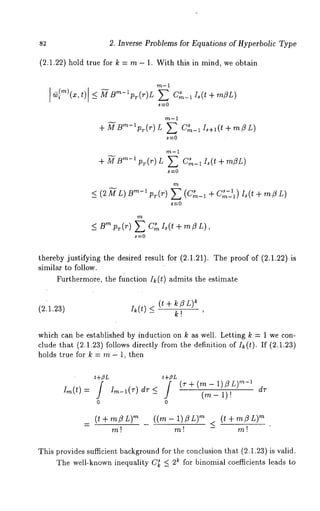
![2,1. Inverse problems for x-hyperbolic systems 83
the chain of relations
k k
~ C~ I,(t) < ~ s~ ( t + s~L)
-
s=0 s=0
~ (~t + ~ZL)
<E2 ~-
~=0
< 2~ ~ (~~ + ~ZL)
-
= 2t exp {t + k~L}.
Putting q = 2 B exp {3/3 L} and replacing T by T + k/3L, we deduce from
(2.1.21) and (2.1.22)
(2.1.24) pT(A~r) <_ q~ T pT+~zr(r).
We now proceed to estimate the seminorms of the element r0.
stated above,
~i(~; x,t) _< t+ ~ZL
and, therefore,
As
I ¢i(T/(x,t)) I _< a exp {aT/}
_< a exp {at + a~L}
= a exp {a~L} exp {at}.
Since the values ODij/Ot, Ori/Ot and O~/Ot are bounded,
I ¢i(x,t) l ~ Co exp {at},
yielding
(2.1.25) p~(~o_)< ~ , exp{ ~T }.
All this enables us to estimate the memberso f Neumann’se ries in (2.1.17).
From (2.1.24)-(2.1.25) it follows
pr(Akro) <_ c~ ekx. p{(o~+ 1)T) [q exp{aC3L)]](https://image.slidesharecdn.com/0824719875inverse-141031173353-conversion-gate01/85/0824719875-inverse-104-320.jpg)
![s4 2. Inverse Problems for’Equations of Hyperbolic Type
With the aid of the last inequality we try to majorize the series in (2.1.17)
by a convergent geometric progression keeping q exp {ct ~ L} < 1. Having
stipulated this condition, the series in (2.1.17) converges uniformly over
0<t<Tand
cl exp {(~ + i)
(2.1.26) Pr(r) -< ~ -- ~ e--~p ~-~-}
It follows from the foregoing that (2.1.17) is just a solution to equation
(2.1.16) and this solution is of exponential growth in agreement with rela-tion
(2.1.26).
The quantity q exp {a~L} of the form
4~L max {1,~H(x,0)-~]} exp{3ZL}exp{aZL}
is continuous and monotonically increasing as a function of L and vanishes
for L = 0. Hence there exists L0 > 0 such that for L < L0
q exp {a~L} < 1
and, therefore, the inverse problem at hand possesses a solution of proper
form. Thus, the theorem is completely proved. ¯
Theorem 2.1.3 Let D, H, Dt and Ht be continuous functions and let K
be a continuously differentiable function. If
IIDII_<MI, ID, II_<M,I IH, II_<M,
It K II I det H(z, 0) l >_ 7 >
with certain positive constants M, fl and 7, then for any b > 0 there exists
L1 > 0 such that for L < L1 the inverse problem (2.1.2), (2.1.8), (2.1.9) can
have at most one solution in the class of functions satisfying the estimate
Proof This assertion will be proved if we succeed in showing that the
homogeneouse quation corresponding to (2.1.16) has a trivial solution only.
Let r=Arand
exp
Since A~ r = r, relation (2.1.24) implies that
(2.1.27) p~(r) = p~(A%) ~ c~ [q exp{bZL}] ~ exp{(b+ 1)r}.
Hence, if we choose L1 so as to satisfy q exp{b~L} < 1 for L < L1, then
the relation pr(r) = 0 is attained by letting k ~ ~ in (2.1.27) and is valid
for any T. But it is possible only if r = 0 and thereby the theorem is
completely proved. ¯](https://image.slidesharecdn.com/0824719875inverse-141031173353-conversion-gate01/85/0824719875-inverse-105-320.jpg)
![2.1. Inverse problems for x-hyperbolic systems 85
Of particular interest is the situation in which the matrix K has fixed
sign. Under the assumption imposed above the existence and uniqueness of
a solution of the inverse problem concerned are obtained for any L. For the
sake of definiteness, the case of negative eigenvalues will appear in more a
detailed exposition.
Theorem 2.1.4 Let D, H, Dt and H~ be continuous functions and let ~, ¢
and K be continuously differentiable functions. One assumes, in addition,
that
II ¢’(t)II < a exp {at}, ~ det H(z, 0)[ ~ 7 > O, ~(0) = ¢(0),
-~(z,t)~ ~ ~ (l<i<n)
with certain constants M, fl, 7 and a. Then in ~he domain ~ the inverse
problem (2.1.2), (2.1.8), (2.1.9) has a solution
V e1, C p e C, II v,I I ~ c exp{ b~)
andI biss olulioies uniquien ~hei edicalcelda sso f fu~clions.
ProofT hep roofo f the existencoef a solutiounn dert he abovea greements
is carrieodu ta s usuM.T hisa mounttso fixinga point( ~,~ ) ~ D and con-siderincgh
aracteris(t2i.ci .i0)U.p oni ntegratianlgo ngt hisc haracteristic
we arrivaet relatio(n2s. 1.IIa)n d( 2.1.12)w,h erea ]]t he~ {’sa ree qual
zero.A fterd ifferentiatwien gge tt hes ystemo f equation(s2 .I.14)-(2.1.15)
of thes econdk indw hichc anb e rewritteinn the concisfeo rm( 2.1.16).
Thei deab ehindd erivatioonf thee stimateisn questioins to refer,
in additiotno the operatoIr, to anotheirn tegratioopne ratoJr witht he
V~Iues
0
Thes ymbolJ } (~)s tandsf ort he functiondse finebdy the recursion
~0(~) ~ J~(~) = ~(~_a(~)).
Usingt he well-knowenx pression
mk
J~(~)=](https://image.slidesharecdn.com/0824719875inverse-141031173353-conversion-gate01/85/0824719875-inverse-106-320.jpg)
![86 2. Inverse Problems for Equations of Hyperbolic Type
we replace (2.1.21)-(2.1.22) by the following estimates:
k
I t~}~)(x,t)[ _< ~pr(r) J ~(z) E C~/~(t +
k
I < B J (x) Zs( + ZL).
s:0
In this line, one useful inequality
p~(A~r) ~_ ex pTpT+k~L(r)
will be involved in place of (2.1.24) and will be useful in the estimation
the sum of Neumann’s series:
pT(r) < C~ exp {(a+ I)T) [qexp{aflL)]k
-- k!
k:O
----- C1 exp {q exp {a~L}} exp {(a + 1)T}.
Further reasoning is similar to the proof of Theorem 2.1.2.
To prove the uniqueness here one should reproduce almost word for
word the corresponding arguments adopted in proving Theorem 2.1.3 by
replacing the value [q exp {b~3L}]k by [q exp {bflL}]~/k !. As k --~ cx~, the
last sequence tends to 0 for any L, thereby justifying the assertion of the
theorem. ¯
In view of the solution uniqueness established for the inverse problem
of finding the right-hand side function, one can easily prove the uniqueness
theorem for inverse problems of recovering other coefficients of the govern-ing
equations. The methodology of the considered problem provides proper
guidelines for subsequent investigations.
Let us"consider the nonlinear inverse problem of finding a matrix
D = D(x) built into the system (2.1.2). As the total number of unknown
coefficients dij(x), 1 < i < n, 1 <_ < n, of thematrix D is equalto n 2,
it is reasonable to absorb more information on the boundary behavior of n
solutions of the system
(2.1.28) {v(~)(x,O)=~(k)(x), O<x<L,
v!~)(O t)= ¢i (x) t>O l<i<s l<k<n
v (L, ¢i (), t>0,_ s<i<n.,_ l<k<n.](https://image.slidesharecdn.com/0824719875inverse-141031173353-conversion-gate01/85/0824719875-inverse-107-320.jpg)
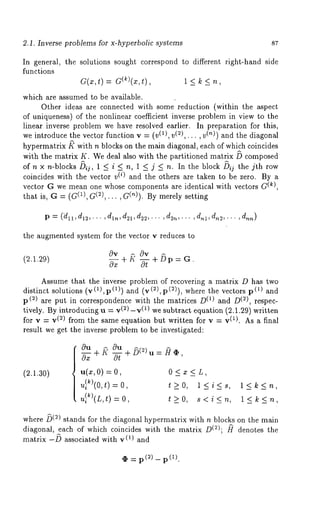
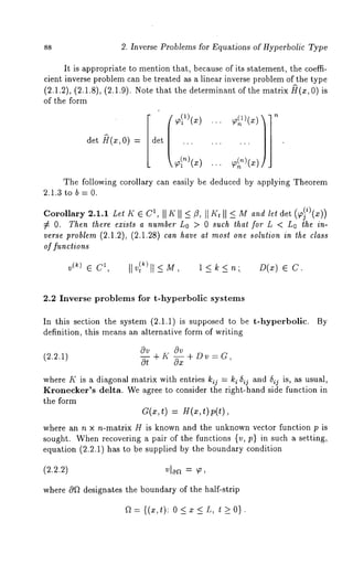
![2.2. Inverse problems for t-hyperbolic systems 89
The function ~(x,t) is assumed to be continuous on 0f~ and the functions
~(0, t), p(x, 0) and ~(L, t) are supposed to be continuously differentiable.
Let the eigenvalues of the matrix K obey the same properties as before.
Recall that ki(x , t), 1 < i < n, are bounded and continuously differentiable
in f~, ki < 0 for 1 < i < s and ki > 0 for s < i_< n. In addition, they
are supposed to be bounded away from zero, that is, there exists a positive
constant c such that I ki(x,t)] >_ c, 1 < i < n, for all (x,t) E ft.
Along with the function ri ((; x, t) being a solution of problem (2.1.10)
we deal with the function ~i(r; x,t), which for fixed values z and t gives
the inverse function of ri(~; x, t) and satisfies the system
(2.2.3)
= ,
= x.
After integrating along the characteristics specified by (2.2.3) the inverse
problem (2.2.1)-(2.2.2) reduces to a system of integral equations.
(ai(x,t),13i(x,t)), 1 <_ i indica te a poin t at whi ch the ch aracteris-tic
(2.2.3) intersects the boundary Oft and ¢?i(x, t) _< t. Putting
,(bi(x,t) = pi(ai(x,t),~3i(x,t)) l<i<n,
we integrate the equations of the system (2.2.1) along the characteristic
establish the representations
t
(2.2.4) vi(z’,t )-~i(x,t)= / (-Dv+Sp) i dr, l<i<n.
~i(~,t)
The next step is to define the numbers 7i as follows: 7i = 0 for 1 < i < s
and 7i = L for s < i _< n and then set Q(t) = ~i(Ti ,~), 1 ~ i ~_ ft.
Furthermore, substituting into (2,2.4) x = 0 for 1 < i < s and x = L for
s < i _< n yields
t
(2.2.5) ei(t)- q~i(’h,t) = f (-Dv + Hp)~ dr, 1 <
fli(’Yi ,t)
The new variables
iOV
wi= Ox
l<i<n,](https://image.slidesharecdn.com/0824719875inverse-141031173353-conversion-gate01/85/0824719875-inverse-110-320.jpg)
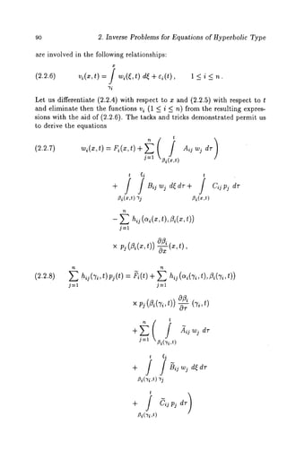
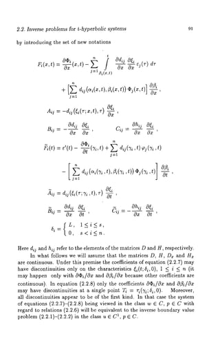
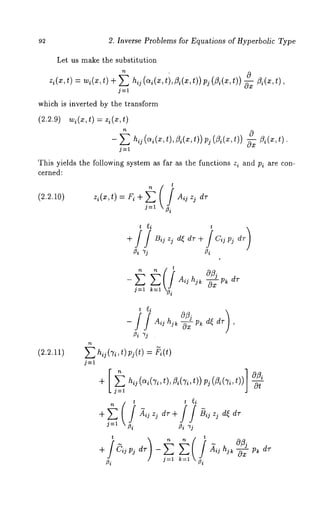
![2.2. Inverse problems for t-hyperbolic systems 95
where t2 > tl, etc. By regarding the spacing
to be fixed we look for a solution of the inverse problem in every domain
Gk = {(x,t): 0 < z < L, tk_l <_ t <
by means of which it is possible to construct a solution of (2.2.1)-(2.2.2)
from the required class everywhere over fL
Setting
p = sup Ik~(z,t)
z, tED
l<i<n
we are exploring the inverse problem (2.2.1)-(2.2.2) in the rectangle
G= {(x,t): O<x< L,O<t <L/p},
bearing in mind that the boundary function is unknown at the point
t = L/p. Now ~i(Ti ,t) =_ (1< i < n)and t his considerably simpl ifies
equations (2.2.11) responsible, in the present framework, for the develop-ment
of the Volterra integral equations of the second kind.
The system of equations (2.2.10)-(2.2.11) written in the vector
(2.2.15) can be solved by means of successive approximations satisfying the
recurrence relations
r(°) = r0 , r (k) (=~ -r01. )+ U r
Owing to the choice of the initial approximation and further iterations
the functions z!~)(x t) may have discontinuities of the first kind on the
characteristic
x = ~(t; 5~, 0),
whereas the functions ~(t) and all the approximations pl~)(t) should be
continuous on the segment [0, L/p].
In mastering the difficulties involved due possible discontinuities of
the functions z}~)(z,t), we try to adapt the functions wl~)(~,t) specified
by (2.2.9):
(2.2.9’) w!~)(x t)=z}~:)(x,t)- hij(c~i(x,t),/~i(x,t))
j=l
× f~)(~(~,t)) -~2](https://image.slidesharecdn.com/0824719875inverse-141031173353-conversion-gate01/85/0824719875-inverse-116-320.jpg)

![98 2. Inverse Problems for Equations of Hyperbolic Type
To complete the proof, we introduce a Banach space M(G) consisting
of all vector functions
~= (z,p)= (zl,..., z,,pl,...
the first n components of which are measurable and bounded in the domain
G and the remaining n components are measurable and bounded on the
segment [0, L/p]. Developing the recurrence relations for (5(k),/5(k))
(2(~-1),15(~-1)) from equations (2.2.10)-(2.2.11) and
U~ r= (2(~), ~(k)),
we get the standard Volterra estimates
- k! It, M(G)I,
Ufi(~)ll < (Mok! t)~ Ir, M(G)
where the norm of an element r = (z,p) on that space is defined by
Ir, M(a)l= max{sup Ilzll, sup Ilpll}.
G [0, L/#]
All this enables us to estimate the norm of the kth power of the operator
U in the space M(G) as follows:
(kMo T)
(2.2.18) IIU~ll _< ~! ,
where T = L/#. From (2.2.18) it is clear that for all sufficiently large
the operator U~ becomes a contracting mapping. In turn, this property
ensures the convergence of the sequence {r(~)} to an element (z, p) e M(G)
in the M(G)-norm. That is to say, the uniform convergence of the sequence
{z(~)(x, t)} to the function z(x, t) over the domain G and the uniform con-vergence
of the sequence {p(k)(t)} to the function p(t) over the segment
[0, tl] occur as k --, ec. In view of (2.2.9’), the functions {w(~)(x, t)}
verge uniformly over G and the limiting function w(x,t) will be related
with z(x,t) and p(t) by (2.2.9). The latter can be derived from (2.2.9’)
by passing to the limit. The functions w(x,t) and p(t) being continuous
must satisfy (2.2.7)-(2.2.8). This proves the existence of the inverse prob-lem
solution. The uniqueness here follows from the contraction mapping
principle. ¯](https://image.slidesharecdn.com/0824719875inverse-141031173353-conversion-gate01/85/0824719875-inverse-119-320.jpg)
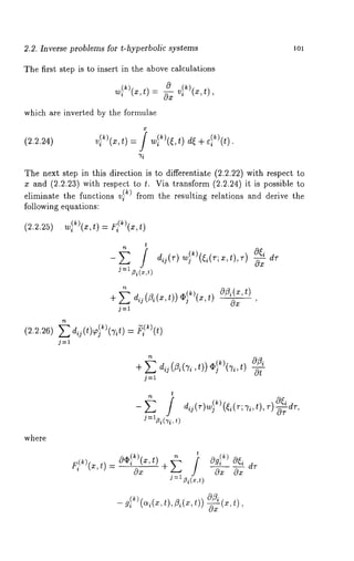
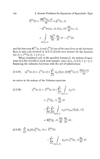
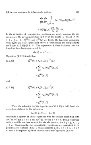
![lO4 2. Inverse Problems for Equations of Hyperbolic Type
Theorem 2.2.2 Let K ~ C1, II K II ~- M, ki < 0 for 1 < i < s, ]~i > 0
for s < i ~_ n, and let ]]~i(x,t)] >_ c > O, 1 < i < n. Let ~(~)(x,t)
~a(~)(0, t), ~(k)(L,t), ~(~)(x,0) ~ ¯ g(~), g(~ ) ~ C and, in ad dit
det (~Ik)(L,t)) ~ 0 s = 0,det ( ~al~)(0,t)) ¢ 0 anddet (~ al~) (L,t)) ¢ 0
for0<s<nd, et( (0,t)) # O for s = n. Onea ssumetsh at the
compatibility conditions (2.2.31), whose ingredients aij(O) are replaced by
their values from equations (2.2.30), hold. Then there exist a time T > 0
such that for t <_ T the inverse problem (2.2.19)-(2.2.20) has a solulion in
the class of functions
v(~)G 1 1 <k<n" D ~ C
Proof By exactly the same reasoning as in the proof of Theorem 2.2.1 it
is convenient to operate in the domain
ar = e a, t < T}
and the space M(f~7,) of all bounded measurable functions
r = {Z(1)(x,t),... ,Z(n)(x,t),
with the norm
Ir, M(~IT )= max{ llz(1)(x,t)ll,... ,llz(~)(m,t)l], IlD(t)
(Tx,t)~a
Let an operator U be defined by integral terms in relations (2.2.28)-
(2.2.29). We choose the "initial" element r0 in such a way that the system
of equations (2.2.28)-(2.2.29) can be written in the form (2.2.15),
ing it possible to solve the governing system by appeal to the successive
approximations
r(0) ---- r0 , r (m) : r o + U r(m-l) m = 1, 2,
Observe that the functions z(k)(m)(x,t) may have discontinuities of the
first kind on the characteristics, while the functions D(’~)(t) should be
continuous. By merely setting t = 0 in (2.2.29) it is easily verified that the
values D(’~)(0) do not depend on m and coincide with the system (2.2.30)
solution. With the aid of (2.2.27) we construct the approximations for
w(~)(z, t), 1 < k < andobserve that the n ew functions turn out t o be
continuous in f~T by virtue of the compatibility conditions (2.2.31).
The current proof differs from that carried out in the preceding theo-rem,
since the system (2.2.28)-(2.2.29) is nonlinear and its solution can
shown to exist, generally speaking, only for sufficiently small values of the
variable t. This completes the proof. ¯](https://image.slidesharecdn.com/0824719875inverse-141031173353-conversion-gate01/85/0824719875-inverse-125-320.jpg)
![108 2. Inverse Problems for Equations of Hyperbolic Type
By the replacements
r I ~72~ l(v r2:~ a
r2 = ~ -- W
we are led to the canonical form
rt=Krx+Dr+o,
where
(rl) a 0 ,
0 --a
D= ~a tac + a% - a
ac - aax - at
at
tac + aa~ -- a , (~ = ~a F .
ac - aax [’
Additional information provides the validity of the relations
0<i<n,
yielding
(2.3.8) a(xi ,t) [r2(xi ,t) + r~(xi ,t)] = X’i(t), l<i<n.
Keeping the integral along the characteristic
t
Li(x,t) 0
i= 1, 2,
and the new parameters
d
B=-- C-
2a ’
ac + aax - at
22a
E = ac - aa~ - at
22a
P --- (Pl ,... ,Pn), g= (gl,..., Pg= L Pigi,
i=1](https://image.slidesharecdn.com/0824719875inverse-141031173353-conversion-gate01/85/0824719875-inverse-129-320.jpg)
![2.3. Inverse problems for hyperbolic equations of the second order lo9
we prefer to deal with concise expressions which are good enough for our
purposes. Other ideas are connected with integral equations which are
capable of elucidating many of the facets of current problems. The first
equation is obtained by integrating the equality ut = v as follows:
t
(2.3.9) u(x, t) = ~o(x) + / v(x, dr.
0
Let us integrate the second and third equations of the system (2.3.8) along
the corresponding characteristics and then add one to another. Multiplying
the resulting expressions by a(x,t) and taking into account the relation
a(rl + r3) = v, we arrive at
(2.3.10) v(x,t) = R(x,t) + a(x,t)
+ f (Bu+Ev+ gp)],
L~(~,t)
where
Since
R(xt,) =a(x,t) 0) +
H- a(x,t) (~a) + (~aa
, . ,t) L~.(x,t)
~’~(,, 0) = 1g-/a ~(*) ~ 1~’(*)
and
1 1
~(~, 0) = ~a ~(x) - ~ ~’(~)
one might expect that the function/~(a:, t) is known. The remaining integral
equations can be derived by merely inserting x = xi, 1 < i < n, in (2.3.10).
By the same token,
(2.3.11) X’i(t) = R(xi ,t)+ a(xi ,t)
~(](https://image.slidesharecdn.com/0824719875inverse-141031173353-conversion-gate01/85/0824719875-inverse-130-320.jpg)
![11o 2. Inverse Problems for Equations of Hyperbolic Type
Our further step is to differentiate relations (2.3.9)-(2.3.11). To avoid
cumbersomee xpressions, it is reasonable to introduce the following nota-tions
for the function $’(z, t) of two independent variables:
d
(2.3.12) m~(T,x,t) = ~ m(~(T;x,t),~),
(2.3.13) $’i+2(r, x, t) = 9~(~i d~i
’ dx ’
d
(2.3.14) ~+4(r,x,t) = ~ ~(~,
(m3.5 ) = , ~.
In formulae (2.3.12)-(2.3.15) the subscript i takes the values 1 ~nd 2.
intervention of a new unknown function z(x, t) = v~(x, t) = u~t(x, t) com-plements
the notation of the integral ~long characteristics. If U(r, x, t)
an arbitrary function of three variables and X(x,t) refers to each of the
functions u, v, w, z and p, one trick we have encountered is to ~dopt
t
Li(x,t) 0
Differentiating relation (2.3.9) with respect to x yields
t
(2.3.16) w(x,t) = ~o’(x) + i z(x, r) d7 ..
0
One more relation, namely,
(2.3.17) z(x,t)-= OR(x,t)Ox + Oa(x,t)Ox [L,ff, t) (Bu+Cv+H~p)
(Bu + Ev + Hgp)] + a(x,t)
L~(x,t)
i=1,2.
+iL~(x,t)](https://image.slidesharecdn.com/0824719875inverse-141031173353-conversion-gate01/85/0824719875-inverse-131-320.jpg)
![2.3. Inverse problems for hyperbolic equations of the second order 111
is a result of differentiating equation (2.3.10) with respect to
Let us introduce one of the integration operators acting in accordance
with the rule
i[7(x,t)] = ] *(~,t/de.
By definition,
and
u(xt, ) =I [w(xt,) ] +x ,(t)
v(~,t) =I[z(x,t)]
and equation (2.3.17) takes the form
(2.3.18) z(x,t) = ¢(x,t) Oa+( x,t)
[ (BIw + CIz + Hgp)
L~~x,t)
+ / (BIw+EIz+Hgp)]
L~(x,t)
+a(x,t)[ / (BllW+Cllz
+ (Hg)l p + Ba w + Ca
+ ] (B2Iw+E2 Iz
+(Hg)~p+B4w+E4z)]
where
7÷,(~,t)- O0R~( x+, t)0 O--a-2(x,t)](https://image.slidesharecdn.com/0824719875inverse-141031173353-conversion-gate01/85/0824719875-inverse-132-320.jpg)
![112 2. Inverse Problems for Equations of Hyperbolic Type
L2(x,t)
+a(x’t)[L(ff~l ,t) (B1XI-~-C1xII)
+ / (B2xI+E2x’I)].
L~(x,t)
Differentiating (2.3.11) with respect to t and denoting by Gij(t), 1 < i <
1 < j < n, the elements of the inverse of (g~(xj, t)), the resulting equations
are solved with respect to the values pi(t), < i < n, lea ding to the
decompositions
~ Oa(x_!jt, )
(2.3.19) pi(t) : Hi(t) - ~ Gij(t)
Ot
j=l
[
x ] / (BIw + CIz + (Hg)
LI(~j ,t)
+ / (BIw + EIz + (Hg)p)
L~(xj ,t)
+a(xj,t)[~j(B5Iw+C5IZL~(,t)
+ (Hg)~ p + B7 w + C7 z)
+ / (B6Iw+E61z
L~(xj ,t)
where
+(Hg)6p+Bsw+Egz)]},
Hi(t): Gi j(~) [~ /i/(t) £gI{(~j,~)Ot
d(xj’t) Xj(t)
j=l](https://image.slidesharecdn.com/0824719875inverse-141031173353-conversion-gate01/85/0824719875-inverse-133-320.jpg)
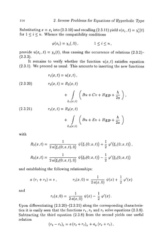
![2.3. Inverse problems for hyperbolic equations of the second order 115
which, with via substituted for r2 + r3, reduces to
(~ - ~3), = vx = z.
Since wt = z and
r~(x,0 ) - r~(x,0 ) = ~’(~)= ’w(~,
we might have
and, therefore, the system of equations written initially is a corollary of
(2.3.8) and can be derived from it by the inverse replacements
u=rl, v=a(r2+r3), w=r~-r3.
However, the second equation of this system represents an alternative form
of writing equation (2.3.1). Thus, the equivalence between the system
(2.3.16), (2.3.18), (2.3.19) and the inverse problem concerned is proved.
The system of equations (2.3.16), (2.3.18), (2.3.19) can be solved
the method of successive approximations. This can be done using the space
C(~) of all vector functions having the form a = (w, z, p), where w
z are defined and continuous in the domain ~ and the vector p(t) of the
dimension n possesses the same smoothness on the segment [0, T]. The
norm on that space is defined by
(2.3.22) Ilall--max{ ~x twl, ~x Izl, m~
[o,
We refer to the vector
a0 = (~a’(x), ¢(x, t),
and an operator L in the space C(~) to be defined by the group of uniform
terms on the right-hand sides of relations (2.3.16), (2.3.18) and (2.3.19),
by means of which the system of integral equations can be recast as
(2.3.23) a = a0 + L a.
In the light of the theorem premises the coefficients of equations (2.3.16),
(2.3.18) and (2.3.19) are really continuous and, therefore, bounded in
domain ~. Taking into account the obvious inequality
one can derive the usual estimates for the Volterra equations:
(~NT)
II L~ all < ~ I1~11,
which can be justified by induction on k. The use of the contraction map-ping
principle implies the existence and uniqueness of the equation (2.2.3)
solution. With the equivalence established above, the same will be valid
for the inverse problem (2.3.1)-(2.3.4), thereby completing the proof of
theorem. ¯](https://image.slidesharecdn.com/0824719875inverse-141031173353-conversion-gate01/85/0824719875-inverse-136-320.jpg)
![116 2. Inverse Problems for Equations of Hyperbolic Type
By means of substitution (2.3.5) from Theorem 2.3.1 we derive one
useful corollary.
Corollary 2.3.1 Let 0 < a(x,t) < M, a(x,t) 2, ¢(x) ¯ C 1 and l et
~(x), Xi(t) 2, 1 < i < n.One assumes, in ad dit ion, that ~(xi) = xi(O
and X~i(O) = ¢(xi), 1 <_ i <_ n. Let the functions c(x,t), d(x,t), h(x,t)
and gi(x,t), 1 < i < n, be continuous along with their first x-derivatives
the domain f~ and let b(x,t) ¯ 2, det (gi(xj , t)) 7 ~ O. T hen t here e xists a
solution of the inverse problem (2.3.1)-(2.3.4) in the class
2u , ¯ C pi ¯ C , l < i < n ,
and ibis solution is unique in the indicated class of functions.
The results obtained permit us to give a definite answer concerning
the uniqueness of recovering other coefficients of equation (2.3.1). Two lines
of research in the study of second order hyperbolic equations are evident
in available publications in this area over recent years. Not much is known
in the case of the combined recovery of the coefficients a(t), c(t), d(t) and
the function u(x, t) satisfying the relations
(2.3.24)
~ttt ~ a~uxz + cut q- du,
u(x, o) ~(x),
u,(~, 0) = ¢(~),
u(~, t) = x~(t), 1<i<3,
where the variables x and t are such that the point (x, t) should belong
the domain ~T described at the very beginning of this section.
Let both collections
(u(1), a(1), c(1),
and
(u(~), a(2), c(2),
solve the inverse problem we have posed above. Setting A(i) = [a( i)] 2 and
v = u(~) - u(1) and subtracting relations (2.3.24) written for u = (1) and
u = u(~) one from another, we derive the system
(~.3.~5)
Vtt = A(2)vxx + c(2)~ t + d(2)v + F,
v(z,O) =
v~(~,O=)
v(x~,t) = 1<i<3,](https://image.slidesharecdn.com/0824719875inverse-141031173353-conversion-gate01/85/0824719875-inverse-137-320.jpg)
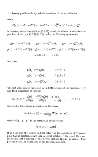
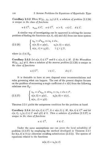
![2.3. Inverse problems for hyperbolic equations of the second order 119
and
can be derived in a similar manner. Relation (2.3.16) remains unchanged,
whereas (2.3.18) should be replaced
(~.3.~s’) z(~,t) = ~(~,t) Oa(z,t)
[
X | I (BIw+CIz+Bx)
LL~~z,t)
+ / (BIw , EIz + BX)*]
La(~:,t)
X
[LlJ, t) (BIIw+CIIz-t-Baw+B1X)
+ / (B~Iw+E~Iz+B4w+E4z+B~x)],
L~(x,t)
where
~(~,t)- O~0(xx, t)+ O a(x,t)
~ ,t) L2(x,t)
~ t) Lz(x,t)
~(x,t) = a(x,t) [r~(~(O;x,t),O) + r,(~(0;x,t),0)
L,(x,t) L~(x,t)](https://image.slidesharecdn.com/0824719875inverse-141031173353-conversion-gate01/85/0824719875-inverse-140-320.jpg)
![12o 2. Inverse Problems for Equations of Hyperbolic Type
Instead of (2.3.19) we arrive at the equation
do(t) at(xl
X(=,t)
X
~ / (Bhv+CIz+
kL~(~ ,t)
+ J (1BIw+EIz+Bx)
~(~ ,t)
a(x~’t) [L ff~ ~ (BsIw+CaIz
)~(t) ~( ,~)
+ B~w + C~z + B5
+ [ (B6 Iw E6 Iz
L~(:c1 ,t)
+Bsw+ Esz + B6X)]
where
Co(t) a(x~ ,t) c(x~ ,t) - at(x~ ,t)
a(~, t) x(t)
Evidently, relations (2.3.16), (2.3.18’) and (2.3.19’) constitute a system
the second kind nonlinear integral Volterra equations. If the coefficients
of the preceding equations are continuous, this system possesses a unique
continuous solution for all sufficiently small t. In concluding the chapter
we give the precise formulation of this fact.](https://image.slidesharecdn.com/0824719875inverse-141031173353-conversion-gate01/85/0824719875-inverse-141-320.jpg)
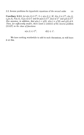

![3. Inverse Problems for Equations of the Elliptic Type
as the potential of a volume mass with density # under the natural
premise that #(y) # almost everywhere inf~. It i s k nown that the v olume
potential u so defined obeys the following properties:
(3.1.6) if# 6 L~(9)
(3.1.7)i t, 6 Ch(~)0, < h
(3.1.8) As Ixl-~
where
then u ~ CI+~(R~)
{-~(x), x~, then Au(x) = O, x ~
log u(z)-~M, n=2,
~ ~-~(~) ~ M, n ~ 3,
M= l
"_~- n(’~-
#(y) dy, n >_
Here the symbol ch((~) is used for the H61der space formed by all continu-ous
on l) functions satisfying H61der’s condition with exponent h, 0 < h
1. The norm on that space is defined by
(3.1.9) sup l u(x)]+Hh(u),
where Hh(u) is Hhlder’s constant and, by definition,
Hh(u): sup {[u(x,)-u(x2)[" 1 -- g2t-h}.
~71, ~2 ~’~
In addition, cl+h((~), l ~ N, 0 < h < 1, is a space comprising all
functions with the first l derivatives which are Hhlder’s continuous with
exponent h.
The potential of a simple layer is given by the relation
(3.1.10) v(x) =/ E(x,y)~(~)
where the integrable density p(y) # al most ev erywhere on 0~. The
function v(x) defined for x ~ Rn c~f~ is twice continuuosly differentiable
and satisfies the Laplace equation, that is, A v(x) = 0 for x ~ Rn cgfL
Moreover, in the case where p ~ L~(Of~) tnh)e function v belongs to Ch(R](https://image.slidesharecdn.com/0824719875inverse-141031173353-conversion-gate01/85/0824719875-inverse-147-320.jpg)
![3.1. Introduction to inverse problems in potential theory 127
for any h, 0 < h < 1. Note that if the function p is continuous on 0f~, then
for the simple layer potential the jump formulae are valid:
(3.1.11) ( Ov )+ OE(xo,y) p(y) dsy,
0~
0v ( 0v ~
(
0v -(x0) denote the limits of ~uu~0 as x -+
where 0~o] (Xo) and 0u~o
(x0 E O~) taken along the external and internal normal ~xo with respect
to fl, respectively.
3.2 Necessary and sufficient conditions for the equality of
exterior magnetic potentials
This section focuses on establishing several preliminary assertions which
will be used in the sequel.
Let finite domains ~, a = 1,2, be bounded by piecewise smooth
surfaces cWG, (~a C Do, where Do is a bounded domain in the space ~
with a piec~wise smooth boundary 0~. The potentials of volume masses
and the potentials of simple layers are defined as follows:
(3.2.1) uS(x) = u(x; fG,#a) = / E(x,y)#~(y)
and
(3.2.2)
0~
Let real numbers fl and 3’ be such that f12 + ~2 ¢ 0. By a generalized
magnetic potential we mean the function
(3.2.3)
If A1 and A2, fi,~ C Do, a = 1,2, are open bounded sets, each being a
union of a finite number of domains
(3.2.4) ~A,~ = U al A2= [.J a~,
j=l j=l](https://image.slidesharecdn.com/0824719875inverse-141031173353-conversion-gate01/85/0824719875-inverse-148-320.jpg)
![128 3. Inverse Problems for Equations of the Elliptic Type
where rnl and m2 are fixed numbers, cOQ[ and 0f~ are piecewise smooth
boundaries, OAc~, ct = 1, 2, is the boundary of As, we will replace f~ and
0f~ by As and cOAc~ everywhere in (3.2.1)-(3.2.3).
Let D be an arbitrary domain (in general, multiply connected) and
let
(3.2.5) Do D
The symbol D1 stands for a domain having a piecewise smooth boundary
such that
(3.2.6) D D/)1, mes(OD1 ClOAk) = O, a = 1,2.
Let h(y) be a regular in D solution of the Laplace equation
(3.2.7) Ah(y) = y E D.
For the purposes of the present chapter we have occasioll to use the func-tional
J(h) with the values
J(h) =/3 [ tt a(y) hi ) dy
A,(Do~)~)
(3.2.8)
A2(DoDa)
+7
OAa(Do~)
- / p:(y) h(y)dsu],
OAA(Do~)
where #~ and p~ are bounded integrable functions.
Lemma 3.2.1 If h(y) is any of the regular in D solutions to equation
(3.2.7), then the functional J(h) specified by (3.2.8) admits the representa-tion
(3.2.9) J(h) = - / M. [w(x); h(x)] ds~
ODx](https://image.slidesharecdn.com/0824719875inverse-141031173353-conversion-gate01/85/0824719875-inverse-149-320.jpg)
![3.2. Necessary and sufficient conditions 129
with
(3.2.10) w(x) = wl(x) - w2(x),
where wC~(x), a = 1, 2, are the generalized magnetic potentials defined by
(3.2.3) and the domains D and D1 satisfy conditions (3.2.5)-(3.2.6). Here
the symbol Mx[w; h] denotes the inlegrand on the right-hand side of the
second Green formula (3.1.3):
0w(x)
Proof If h(y) is any solution to equation (3.2.7), then formula (3.1.5) gives
in combination with relations (3.2.5)-(3.2.6) the representation:
(3.2.11) - [ M.[’(x,y);h(x)] ds.:-(
y E D~,
OD~
where E(x, y) is the fundamental solution (3.1.4) to the Laplace equation.
Multiplying (3.2.11) by ~(y) and integrating over A~ yield
(3.2.12) / ,~(y) h(y)
Changing the order of integration (this operation is correct, since the in-tegrals
on the right-hand side of (~.2.12) have weak singularity; for more
detail see Hunter (~aa)) and retaining notation (a.2.1), we arrive
~a~(Do~D~) OD~
If (3.2.11) i8 multiplied by pa(y) and subsequently integrated over 0A~
with (3.2.6) involved, we thus have
(3.2.14) f pa(y) h(y)dsy=- /p~(y){ fMx[E(x,y);h(x)]
OA.~(DokD,) OA. OD,
OD~](https://image.slidesharecdn.com/0824719875inverse-141031173353-conversion-gate01/85/0824719875-inverse-150-320.jpg)
![3.2. Necessary and sui~cient conditions 131
Granted (3.2.17), we pass to a domain D1 ordered with respect
inclusion:
(3.2.21) D
Any domains D and D1, arising from (3.2.20)-(3.2.21), must s~tisfy (3.2.5)-
(3.2.6) and, moreover,
Therefore, the properties of the potential of a volume mass ~nd those of the
potential of ~ single l~yer along with (3.2.17) imply that in (3.2.9)-(3.2.10)
(3.2.23) ~v[w(x);h(x)] : 0 x G ODa.
Together (3.2.8), (3.2.9) and (3.2.22)lead to (3.2.18) ~nd the
completely proved.
In ~uxiliary lemm~ we agree to consider
(3.2.24) B = (A~ U A2) ~ ~0, A0 = A~ ~
(3.2.25) J(h,A~ ~ Ao,,~,OA~,p~) = p~(y) h(y)
A~Ao
+ f
OA=
Lemma3 .2.3 For the equality
(3.2.26) w(x;Al,#~,OA~,pl)= w(x;A2,#2,0A2,p2),
to be valid il is necessary and sufficient that the relations
xE D0/~,
(3.2.27) #1(y) = #2(y) for y ~ Ao (if t3 ¢ 0),
(3.2.28) J(h,A~ Ao,#~,OAl,p~) = J(h, A2 Ao,#2,OA2,p:)
hold, where h(y) is any regular solution to the equation
(3.2.29) Ah(y) = O, y ~
and D is an arbitrary domain involved in the chain of inclusions
(3.2.30) Do
Here the set B and the functional J built into (3.2.28) are given by formulae
(3.2.24)-(3.2.25).](https://image.slidesharecdn.com/0824719875inverse-141031173353-conversion-gate01/85/0824719875-inverse-152-320.jpg)
![3.2. Necessary and sufficient conditions 133
and D1 that we have mentioned the functional J(h) can be rewritten as
(3.2.37) J(h)=z[
AI(AoOD1)
- /1 #~(y) h(y)dy
A2(AoV~D~,)
+’)’ [~A~pa(y) h(y)dsyO
- / pz(y) h(y) dsy]’
OA~
under the natural premise 0A~ fq (Do /31) = ~. Since the right-hand side
of (3.2.36) is independent of D1, we are led to (3.2.28) by merely choosing
a sequence of domains {D~},~__I satisfying (3.2.35) such that rues(A0
D~) ~ 0 as n ~ c~. Thus, the lemma is completely proved.
Before giving further motivations, it will be convenient to introduce
the new notations as they help avoid purely technical difficulties. Denote
by f.e the boundary of the set 41 U 4s. In the case f~ ¢ f*~ we thus have
= OA1 r
In what follows we accept ~, = cOA, for c~ = 1, 2 if A1 =
Let B0 be any connected component of the open set B = (AIUA~)40
with OBo being the boundary of B0 and set
Assume that the sets A1 and As are located in such a way that
rues (C~Bo Clr~)=0
for at least one of the domains B0. Without loss of generality we mag
suppose that B0 C (41 40). Within notation (3.2.38), the set f’~](https://image.slidesharecdn.com/0824719875inverse-141031173353-conversion-gate01/85/0824719875-inverse-154-320.jpg)
![3.2. Necessary and suificient conditions 135
implies that
(3.2.48) -
O, y ~ Do D1.
Let us multiply (3.2.48) by #z(x) and integrate then the resulting relation
over the set As A0. Changing the order of integration and retaining
notations (3.2.39)-(3.2.43), we arrive
= [ h(y) .1 (y)
Bo
and
Furthermore, let (3.2.48) be multiplied by p~(y) and integrated over
with regard to (3.2.39)-(3.2.43). Since B0 C (A1 ~), we thus
= f pl(~)h(~)
(OBo)~
--O/D~ M,[ IfA ~ E(x,y)p~(y) ds~);h(x)]
= f p~(~)h(y)ds~.
i(OBo)
Multiplying (3.2.49) and (3.2.51) by fl and 7, respectively, one can add
results, whose use permits us to obtain the relation
(3.2.53) - M~[w(x,A~Ao,#l,0A~,pl);h(x)] ds
OD~
Bo](https://image.slidesharecdn.com/0824719875inverse-141031173353-conversion-gate01/85/0824719875-inverse-156-320.jpg)
![136 3. Inverse Problems for Equations of the Elliptic Type
Likewise, it follows from (3.2.50) and (3.2.52)
(3.2.54) - / Mx[w(x,A2 Ao,l~2,0A2,p~);h(x)]
f
= ~ / p2(y) h(y)
(OBo)~
In conformity with (3.2.44) the proof of Lemm4a .2.3 serves as a basis for
(3.2.34), thereby justifying that the combination of (3.2.34) and (3.2.45)
gives
(3.2.55) w(x;A 1 AO, ~l, G~Al, Pl) : w(x,; 2 Ao, #2 , ~m 2, p2 )
for x E Do [~.
Therefore, the left-hand sides of (3.2.53) and (3.2.54) are equal by virtue
(3.2.55) and the properties of the potentials of volume masses and simple
layers. Thus, the equality of the right-hand sides of (a.2.sa)-(a.~.54i)s
established. This proves the assertion of the lemma. ¯
In what follows we shall need the concept of generalized solution
to the Laplace equation in the sense of Wiener (for more detail see Keldysh
and Lavrentiev (1937), Keldysh (1940)). In preparation for this, we
to the boundary 0ft of a domain ~ (in general, multiply connected) such
that a neighborhood of any point of 0f* contains the points of the set
R’~ ~. Any domain f~ enabling the solvability of the Dirichlet problem
for the Laplace equation with any continuous boundary data falls into the
category of standard domains.
Let a function f(x) be continuous and defined on the boundary c0f~
of a domain f~, which is multiply connected and bounded. The intention
is to .use a continuous function ~(x) defined everywhere in the space ~
and identical with f(x) on 0Q (for more detail see Keldysh and Lavrentiev
(1937)). In what follows we involve a sequence of domains
with boundaries
OD~, @D~, ... , @D,~, ... ,
containing the closed set f~ t2 cOf~ and converging to the dotnain f~, so that
from a certain number m0 and on any closed subset of R~ ~) will be out
D,,~ o. We may assume that the components of c0D,~ are analytical with](https://image.slidesharecdn.com/0824719875inverse-141031173353-conversion-gate01/85/0824719875-inverse-157-320.jpg)
![138 3. Inverse Problems for Equations of the Elliptic Type
As far as the function f(x) is bounded, the extended function ~(x) can
so chosen as to satisfy
’1~~,1, [fl-<M--const in R
[hm~[, [hf[<_M in (~ forany m=l, 2,....
yielding
This is due to the principle of maximumm odulus. The function #(y) being
bounded in (~ provides the validity of the estimate
It(v) ons ,
which is uniform in m. Therefore, by the Lebesque theorem the limit
relation
(3.2.58) ~i~ f ,(y) h~(y)dy = f ,(y) h~(y)dy
takes place. From (3.2.57) it follows that the left-hand side of (3.2.58)
equals zero. Thus, (3.2.56) is true and thereby the lemma is completely
proved. ¯
To assist the readers in applications, we are going to show how the
assertions of Lemmas3 .2.2-3.2.4 can be extended to cover the generalized
solution h] of the Dirichlet problem for the Laplace equation by using
Lemma 3.2.4 ~s one possible example. ~ue, it is to be shown for the
problem
f ~h(~) = 0, ¯ ~ ~0,
(a.2.a9) = ¯ ,
where B0 arose from (3.2.39)-(3.2.41), that any continuous on ON0 function
W can be put in correspondence with a function h~. Being a generalized so-lution
of the Dirichlet problem (3.2.59) in the sense of Wiener, the function
h~ is subject to the relation
(3.2.60) ~h,(~) = ¯ e ~0,
and takes the values ~(x) at regular points of the boundary 0B0, what
means that
lim h~(x) = W(xo), xo ~ OBo is a reg ul ar point ),
irrelevant to the choice of a continuous function ~ (see Landis (1971)).
Note that the generalized solution he is identical with the solution of
the Dirichlet problem (3.2.59) itself, if any.](https://image.slidesharecdn.com/0824719875inverse-141031173353-conversion-gate01/85/0824719875-inverse-159-320.jpg)

![3.3. The exterior inverse problem for the volume potential 141
Theorem 3.3.1 Let the origin of coordinates 0 be enclosed in the set
~1 ~ ~2 and
(1) the radius vector Ru obey the inequality
(3.3.3) (Ru,ny)_>0 for y E s~ , s~ ,
where ny is a unit external normal to the boundary 0~, a = 1, 2,
and (Ry, n~) signifies the scalar product of the vectors Ry and nu;
(2) the exterior volume potentials of the Laplace equation generated by
the domains ~, a = 1, 2, with density # of class (3.3.2) satisfy the
equality
(3.3.4)
Then
Proof We agree to consider ~)0 = ~1 ~1 ~2 with mesFt0 :~ 0. We spoke
above about f~ denoting the domain bounded by the surface s~, for which
the relation (~ = (~1 U ~ takes place.
Together condition (3.3.4) and Lemma 3.2.2 with ~ = 1 and 3’ =
imply the relation
(3.3.5) ] ] = 0
for any function h(y) harmonic in the domain D D ((~1 fl ~).
In further reasoning the contradiction arguments may be of help in
achieving the final aim. We are first interested in the case where 5(y) =
which admits comparatively simple proof. To put it differently, the positive
function #(y) ~ C~((~ Cl ~)2) must satisfy the inequality
(3.3.6) 0 (rn#) 0 Cr 9¢- ~0 y~ ~=~...1~. J~=~2 ~t > ~
By merely setting h = 1 in (3.3.5) it is easily verified that the masses
of the bodies ft~ and f~ are equal in that case. Therefore, due to the
positiveness of the density neither of the domains f~a will be strictly inside
another. Because of this fact, another conclusion can be drawn for the
domains f~; and ft~ with different connectedness that their mutual location
together with (3.3.3) guarantees that either of the sets s:,, c~ = 1, 2, will
be nonempty.](https://image.slidesharecdn.com/0824719875inverse-141031173353-conversion-gate01/85/0824719875-inverse-162-320.jpg)
![144 3. Inverse Problems for Equations of the Elliptic Type
we might select a monotonically increasing sequence of functions {f~ (y)} k=,
being continuous on st such that
f +l(y) >
Here 7k(Y) refers to a continuous function whose values range from 0 to
For every continuous on s t function f~:(y) the generalized solution
HA of the Dirichlet problem is introduced to carry out more a detailed
exploration. Since
f~+i(Y) >- f~(Y), y ~,
the principle of maximumm odulus with respect to the domain f~e implies
that
(3.3.14) HIk+l (Y)
In so doing, [H~,k [ < 1.
As a matter of fact, {HI~ }¢° is an increasing sequence of functions k--1
which are bounded in f~* and harmonic in f~*. By Harnack’s theorem this
sequence converges to a function HI uniformly over f~e and the limiting
function appears to be harmonic in ~*. The convergence HI~ (y) --, I (y)
occurs for all y ~ ~)1 U ~)2. Using the results ascribed to Keldysh and
Lavrentiev (1937), Keldysh (1940) we see that the function HI~ takes
values f~(y) on s t at any point of the stability boundary. Due to this
property the construction of f~(y) guarantees that the limiting function
HI(y) takes the values f(y) on the boundary a~ except for a set of zero
measure.
When k is held fixed, the sequence {Hm~ }~:~, by means of which
we have defined the function HA in Section 1.2, converges in the closed
domain f~ and I tIm~k I < 1 for m = 1,2,.... Hence the Lebesque theorem
on the passage to the limit yields
lim )J(Hm~,~)= J(HI~
for any fixed k.
The function H]~, in turn, converges to HI in the closed domain f~
and [ HI~ [ < 1 for k = 1, 2,.... On the same grounds as before, we find by
the Lebesque theorem that
lim J(HIk ) = J(HI).
Because of (3.3.10),
J(H,~%) =](https://image.slidesharecdn.com/0824719875inverse-141031173353-conversion-gate01/85/0824719875-inverse-165-320.jpg)
![3.3. The exterior inverse problem for the volume potential 145
for any fixed k and m = 1,2,.... Consequently, Y(/-/]~) = 0 for any k,
that
/3.3.15) J(Hf) =
where the function //] is harmonic in ~ and takes the boundary values
equal to flY) from (3.3.11) almost everywhere. Moreover,
/3.3.16) 0 < H~, < 1.
In continuation of such an analysis we refer to the functional
with the values
e
s~ U s~
(3.3.17)
Since
HI #(y) (Ry, ny) ds~
-/
82 U 81
H! #(y) (Ry, nu) ds~
]
k--1
(3.3.18)
a-~
n# + r ~rr
:r n-1 ~ ’
condition (3.3.6) assures us of the validity of the inequality
(3.3.19) ~--~-y~(#y~) >0, when r¢0 foryE~lU#t~.](https://image.slidesharecdn.com/0824719875inverse-141031173353-conversion-gate01/85/0824719875-inverse-166-320.jpg)
![3.3. The exterior inverse problem for the volume potential 147
The preceding manipulations are based on the well-known decomposition
fh f~0
-- / # (Ry, ny) dsy ,
i
82
where ny is a unit external normal to the boundary cOf~ for a = 1, 2.
In accordance with what has been said, the function HI takes the
boundary values f(y) almost everywhere on se= sle U s~.e In view of this,
substituting the data of (3.3.11) into the preceding inequality yields
(3.3.20) J(H])
dy.
Putting these together with relations (3.3.15) and (3.3.19) we deduce
/° z]~ ~E N (. v~) > o.
k----1
Since #(y) > 0 for any y E D1 U D2, the combination of the second
condition of the theorem with (3.3.16) gives
JH] #(y) (Ry,nv) dsv >_ O,
i
81
(1 - H/)#(y) (R~,n~) d% >_ O,
i
82](https://image.slidesharecdn.com/0824719875inverse-141031173353-conversion-gate01/85/0824719875-inverse-168-320.jpg)
![148 3. Inverse Problems for Equations of the Elliptic Type
meaning J(H]) > 0, which disagrees with (3.3.15). Thus, the theorem
its first part is proved.
The situation in which the density #(y) happens to be of nonconstant
¯ sign and satisfies (3.3.2) with items (a) and (b) comes second. In
(b) condition (3.3.4) written for an arbitrary function H(y) harmonic in D
implies relation (3.3.10), that is,
(3.3.21) J(H) = 0,
where
f
J(H) = J H(y)#(y) (Ry,ny) dsy
f
- J H(y)#(y) (Ry,ny) dsy
- H(y)
fh
dy
The well-established decomposition
J(H) = J~,+(H)+ J#-(g)
applies equally well to the following members: the first term J,+(H) com-prises
those parts of integrals in (3.3.21) which are taken over 0~ and
~ ~0, wher~e( y) > 0 for all y ~ fil U~ . Thes econdte rmJ ,-
corresponds to those parts of integrals in (3.3.21) which are taken over
and~ ~0, wher~e( y)_ <0 for all y ~ ~1
Let
0~÷= {~e 0~, ,(~) > 0}; 0~,-= {~ e 0~,, (~) < 0};
(3.3.22)
~+ = {~ e ~, ~(~) > 0}; ~.- = {~ e ~, ,(~) ~ 0}.
Bearing in mind (3.3.1) and the way notation (3.3.22) has been introduced
above, it is possible to produce a number of the new symbols. In particular,
it is fairly commonto use
~ {~e~~. ~. .(~) >0} ~=~,~ S~+ ~
~ ¯](https://image.slidesharecdn.com/0824719875inverse-141031173353-conversion-gate01/85/0824719875-inverse-169-320.jpg)
![3.3. The exterior inverse problem for the volume potential 149
Within these notations, we introduce the function f(y) defined on the sur-face
se = es 1 tO se~ by the relations
1 for yes1,+, s2,-,
(3.3.23) f(Y) = fo r y
Under the premises of the theorem it follows from the foregoing that f(y) k
const for y ~ se. As in the first part of the proof it is necessary to extend
relation (3.3.10)in order to involve the solution Hi(y) of the Dirichlet
problem for the Laplace equation. The boundary values taken by )Hi(y
on 8e coincide with those from (a.u.aa)l most everywhere. In this line, we
obtain
(3.3.24) J(H:) = 0,
where
and
(3.3.25) J/*+(H])
J(H]) = J~,+(HI) + J/*-(H])
1 ¯ #(y) (Ry,ny) dsv
81/,+
i
81#+
HI(y) #(y) (Rv, n~) dsy
-/
i
82/,+
Hi(y) p(y) (R~, ny) dsy
HI(y) 0~- ~
k=l ~Yk (t’tYk)
0HI(Y)[~
dy
dy;](https://image.slidesharecdn.com/0824719875inverse-141031173353-conversion-gate01/85/0824719875-inverse-170-320.jpg)
![150
(3.3.26)
3. Inverse Problems for Equations of the Elliptic Type
Zu-(H]) = / H](Y)#(Y)(Ru’nu) u
dy
i
81#-
82#-
i
82#-
1 ¯ #(y) (Ry,ny)
HI(Y) #(Y) (Ru, u) ds
(~ ~o)#-
+ Hi(y ) ~ -ff~y~(#y~) dy.
(~2 ~o),-
Conditions (3.3.2) in terms of (3.3.22) imply the chain of inequalities
(3.3.27) ~L-~(~y,) >0 for ye(~~o)u+, 4=1,2;
k=l
(3.3.28) ~y~(#y~: <0 for Ye(~a~0)u-, a=l,2.
In view of the bounds 0 < HI < 1 for any y ~ fl*, we are led by relations
(3.3.2), (3.3.27) and (3.3.28) to the estimates
(3.3.29) - Hi(y ) ~ -~y~(#y~)
k=l (~ ~o),+
_> - f ,(v) (R~, ~)
81~+
i
82~+](https://image.slidesharecdn.com/0824719875inverse-141031173353-conversion-gate01/85/0824719875-inverse-171-320.jpg)
![3.3. The exterior inverse problem for the volume potential
(3.3.30) Hi(y) 0
t8-2t
-/
i
81#-
From (3.3.27)-(3.3.30) fo].]ows that
(3.3.31)
(3.3.32)
#(y) (Ry, ny) dsy
,u(y) (Ry, ny) dsy.
151
Taking into account (3.3.3), the properties of the function #(y) specified
by (3.3.2) and the properties of the function Hi(y) revealed in estimates](https://image.slidesharecdn.com/0824719875inverse-141031173353-conversion-gate01/85/0824719875-inverse-172-320.jpg)
![3. Inverse Problems for Equations of the Elliptic Type
(3.3.23), we deduce that every term in square brackets on the right-hand
sides of (3.3.31)-(3.3.32) is nonnegative and, moreover, at least one of
is strictly positive. Thus, we should have J(H]) > 0, violating (3.3.24).
The obtained contradiction proves the assertion of the theorem. ¯
Remark 3.3.1 Condition (3.3.3) of Theorem 3.3.1 is satisfied
is a "star-shaped" set with respect to the point O E ~)1 ~1(~2. For each such
set, R~ (~)1 ~1~2) appears to be a one-component set. In particular,
either of the sets ~1 and (~2 is "star-shaped" with respect to a common
point O, we thus have (3.3.3).
3.4 Integral stability estimates for the inverse problem of
the exterior potential with constant density
As we have already mentioned in preliminaries to this chapter, the question
of uniqueness of inverse problem solutions is intimately connected with their
stability. The general topological criterion of stability ascribed to Tikhonov
(1943) and based on the corresponding uniqueness theorems implies the
qualitative stability tests.
In this section several stability estimates for the inverse problem of the
exterior potential for n _> 3 will be derived in the class of "non-star-shaped"
bodies that consists of the so-called "absolutely star-ambient" and "abso-lutely
projectively-ambient" bodies including those with "star-shaped" in-tersections
and, correspondingly, with boundaries having intersections only
at two points by a straight line parallel to a known direction.
We denote by u(x; A~) = u(x; Ac~, 1) the volume potential of the body
As with unit density. Throughout this section, we retain the notations
given by formulae (3.2.~)-(3.2.4), (3.~.3S) and (3.3.~) and attempt
damental solution of the Laplace equation in the form (3.1.4). In particular,
we agree to consider
1 1
(3.4.1) E(x,y)= 4rr
for n=3andr~y =
As we will see a little later, it will be convenient to deal with
(3.4.2) w(x) = w(x; A~) - w(x;
where
(3.4.3) w(x; d~) =
- (~ + Z~q~) ~](https://image.slidesharecdn.com/0824719875inverse-141031173353-conversion-gate01/85/0824719875-inverse-173-320.jpg)

![154 3. Inverse Problems for Equations of the Elliptic Type
A simply connected domain D.1 with a smooth boundary OD.1 is much
involved in further reasoning to avoid cumbersome calculations under the
agreements that D1 D D./and none of the singular points of both functions
u(x; .~/.a), ~ -- 1,2, lies within the domain/9
One way of proceeding is to refer to the functional
(3.4.8) J(H) = / H(y)~(y) dsy- / H(y)~(y)
where H(y) is an arbitrary harmonic in D function, (I)(y) has been defined
in (3.4.6) and c9~ is the boundary of ~2~ C ~, n>_3, a = 1, 2. Be-fore
we undertake the proof of the theorem, a preliminary lemma will be
introduced.
Lemma3 .4.1 The functional J(H) specified by (3.4.8) admits the estimate
(3.4.9) I J(H)I < c~ max IH(y) max w(x)
-- yEOD1 xEOD .1 ~ ’
where c~ -- const > 0 *de~p. ends on ~he boundary OD
Proof Indeed, any function H(y) harmonic in the domain D D ~ can be
represented in the form
(3.4.10) Mx [E(x,y);g(x)] = 0, y{ ~H R(y), y~ D~, ~ ~ ~,
/
OD~
where E(x, y) stands for the fundamental solution of the Laplace equation
for n ~ 3. The expression for M[u; v] is as follows:
Ou Ov
(3.4.11) M[u;v] = v.(x) On. On~ u(x)
with n~ denoting a unit external normal to OD~ at point z. Furthermore,
we will use as a tool in achieving important results a functional and a
harmonic function which carry out the following actions:
(3.4.12) Y(h) = f h(y) dy- dy
and
(3.4.13) =
k----1](https://image.slidesharecdn.com/0824719875inverse-141031173353-conversion-gate01/85/0824719875-inverse-175-320.jpg)
![3.4. Integral stability estimates for the exterior potential 155
Here H(y) is harmonic in D and the numbers 7~, ~ and q~ have been
defined in (3.4.6). Via representation (3.4.10) for the function H(y) we
might have
(3.4.14) h(y) ey = ~y~ [(7,y~ + ~lqk) H(y)] ey
~, ~, k=l
for a = 1, 2. Using the well-established decomposition for n _> 3
(3.4.15)
k=l
: ~ E(x, ~) - ~ (~ + ~lq~)
k=l
we rewrite the expression in curly brackets from the last formula (3.4.14)
as
(3.4.16)
~ k=l
where the function w(x; ~) has been defined in (3.4.3). Therefore, with
the aid of (3.4.14) and (3.4.16) we establish for any pair of the functions
h(y) and H(y) built into (3.4.13) the relation
(3.4.17) / h(y) dy: / M~[w(x;~.);H(x)]
cOD~](https://image.slidesharecdn.com/0824719875inverse-141031173353-conversion-gate01/85/0824719875-inverse-176-320.jpg)
![156 3. Inverse Problems for Equations of the Elliptic Type
Some progress will be achieved if the function h(y) will be taken in the
form (3.4.13) with further substitution into (3.4.12). As a final result
get the equality
(3.4.18) j(H) J( H),
where the functional J(H) has been defined by (3.4.8). On the other hand,
(3.4.12), (3.4.17) and (3.4.18) imply
(3.4.19) J(H) = / M~[w(z);H(x)]
with w(x) being still subject to (3.4.2)-(3.4.3).
Via representation (3.4.19) one can derive an upper bound for the
absolute value of the functional J(H). In the light of the premises of the
lemma the function w(x) is harmonically extendable from ~ D~to the
domain PC~ D*’. When solving the exterior boundary value Neymann
problem, one can find on the surface cgD*’ the density w(y) of the simple
layer potentiM
(3.4.20) v(x) = / w(y) E(x,y)
OD"
for which
c9 v(x) - cgnx
(3.4.21) [-~n~ ]- 0 w(x) for x e OD*’
,
where v(x) denotes the limiting value of
0 v(:e’) as :e’ OD*’)
On---2
along a unit external normal n, to D*’. In conformity with the uniqueness
of a solution of the exterior boundary value Neymann problem (n >_ 3),
relation (3.4.21) yields
(3.4.22) w(x) = v(x) for x 6 ’~ D*’,](https://image.slidesharecdn.com/0824719875inverse-141031173353-conversion-gate01/85/0824719875-inverse-177-320.jpg)
![3.4. Integral stability estimates for the exterior potential 157
showing the notation w(x) to be a sensible one. Consequently, 3.4.19),
(3.4.20) and (3.4.22) serve to motivate the representations
OD1 0 ’
OD*j ODI
With (3.4.10) in view, the latter becomes much more simpler:
(3.4.24) J(H)= / w(y)H(y) dsy .
OD*’
Thus, the functional J(H) can be estimated as follows:
(3.4.25) IJ(H) I< max lH(y)l ] tw(y) y*E~OD
*O~D
< max Ig(y)l f I~(y)l d%.
y~OD~ J
On the other hand, we should take into account that the function w(y)
solves the integral Fredholm equation of the second kind
(3.4.26) (I - T)~ =
on the basis of (3.4.20)-(3.4.21) and the formulae for the jump of the normal
derivative of the potential of the simple layer. Here I is, as usual, the
identity operator. The operator T and the function f act in accordance
with the following rules:
OE(xy, )
(3.4,27) Tw = 2
On~ w(y) ds~
*O~D
f(x) =-20w(x)
On~ ’
~ E OD*’.
On the strength of the uniqueness of a solution of the exterior Neymann
problem (n >_ 3) the inverse operator (I - -1 should be bounded in the
space of all continuous functions. Thus, (3.4.26 and (3.4.27) imply
inequality
(3.4.28) max lw(y) l < c~ w(z) c2 =- const > 0.
yEOD.~ -- x~OD.~ ~
Estimate (3.4.9) is an immedi’ate implication of (3.4.26) and (3.4.28)
this proves the assertion of the lemma. ¯](https://image.slidesharecdn.com/0824719875inverse-141031173353-conversion-gate01/85/0824719875-inverse-178-320.jpg)
![158 3. Inverse Problems for Equations of the Elliptic Type
We return to proving the theorem by appeal to a function f(y) defined
on the surface se = seI (2 se~ by the relations
-sign(I)(y) for y E
(3.4.29) f(Y) = sign(I)(y) for y G
By means of the function f(y) one can produce a generalized solution
HI (y) of the Dirichlet problem for the Laplace equation in ~uch a way that
HI(y) will be harmonic within ~e, I H~.(y)[ _< 1 will occur for y ~ ~
and the boundary values of HI (y) on the boundary s ~ will coincide almost
everywhere with f(y) involved in (3.4.29). All tricks and turns remain
unchanged as in the proof of Theorem 3.3.1. The way its result is used
here is to select a sequence of functions { gm~ }~=~, l Y~ ~ ~ 1, which
makes it possible to find a function H]~ with relevant properties:
~H]~]~ 1 and HA converges to HI in ~.
Under the conditions of the theorem we are now in a position to consider
the domain D*, D~ C ~, instead of the domain D*~, arising from the
preceding lemma. Since ~* C fie, estimate (3.4.9) implies that
0
(3.4.30) Y(U~) < I J(H~)I < max w(¢)
-- ~ ~EOD* ~
Holding k fixed and passing ~o ~he limi~ in (~.4.~0) as m ~ ~, we derive
~he estimates
(~.4.~) ~(~) < I~(~)~ < ~(~)
-- -- xEOD* ~
~
which after another passage to the limit as k ~ ~ look as follows:
(a.4.a~) j(g~) < ~j(H~)I < c~ max w(z)
-- -- x~OD* ~
On the other hand, the boundary values of HI on s ~ have been defined
by (3.4.29), so that (3.4.8) gives
(3.4.33) / I¢(y) l dsy
S1
+ / I~(y) l dsy
82
+ / HS(y) ~(y) dsy
i
81
i
= J(H]).](https://image.slidesharecdn.com/0824719875inverse-141031173353-conversion-gate01/85/0824719875-inverse-179-320.jpg)
![3.4. Integral stability estimates for the exterior potential 159
Since I H] I -< 1, inequality (3.4.33) is followed
(3.4.34)
- / IcD(y) l d% <_ J(H]).
i
82
Now estimate (3.4.7) is an immediate implication of (3.4.32) and (3.4.34)
with notations (3.4.4)-(3.4.6). This completes the task of motivating
desired estimate. []
We give below several corollaries to Theorem 3.4.1 that furnish the
justification for what we wish to do.
Corollary 3.4.1 Let ~1 ¢ ~2" If there exist a point O, numbers
and a vector q such that
(3.4.35)
i i e e
Sl 82 81 82
then the exterior potentials u(x; 0~) of a constant density cannot coincide,
that is, the set R’~ ( (~1 U (~) encloses a point ~ such
(3.4.36)
Remark 3.4.1 In the case where 71 = 1 and ~1 = 0 we might have
¢P(y) = (Ry, n~) and
(3.4.37) I I(au,n) d% I I(Ru’nYd)%
i i
81 82
_< / I(R~, ny)[ dsy
81
+ / I(R~,ns) d%
82](https://image.slidesharecdn.com/0824719875inverse-141031173353-conversion-gate01/85/0824719875-inverse-180-320.jpg)
![16o 3. Inverse Problems for Equations of the Elliptic Type
instead of condition (3.4.35).
Note that Corollary 3.4.1 is still valid if (3.4.37) is replaced
(3.4.38) ]’ I(Ry,ny), dsy + ] [(Ru,nu)[ dsy
i i
81 82
81 82
It is obvious that (3.4.37) follows from (3.4.38). We claim that (3.4.38)
holds if, in particular, the set {~1 f3 ~2 is "star-shaped" with respect to a
certain point O ¯ {~1 f3 {~2, both sets se a = 1,2, are not empty with
mes (s~ f3 s~) = 0. To avoid generality for which we have no real need,
will consistently confine ourselves to a domain D C R’* bounded by the
surface cqD. Then the volume of D can be expressed by
mesD=-/dy= l /[~-~ OYk ]dy 1/(Ry,ny) dsy
D D k-~l OD
yielding
(3.4.39) mesD = 1 ] (R~,n~) ds~
n
OD
In particular, if the set ~1 f3 ~2 is "star-shaped" with respect to at least
one point O ¯ ~1N~2, mes(s’ 1 f~s*2) = 0 and mess: :/= 0, a = 1,2, then
(Rv, ny) _> 0 on i~, ~= 1,2. Because of (3. 4.39), the mean ing of r elation
(3.4.38) is that we should have
mes(~,~) > mes(~).
Remark 3.4.2 If 7x = 0 and/?~ = 1, then ¢(y) = (q, nv) and condition
(3.4.35) can be replaced
(v3+.4J[.4(q0,)n ~ /)[[(dqs,g ny)[ds
81 82
81 S2
The preceding inequality holds true if, in particular,
mes(
and the intersection of the set s~ ti_ Ji sb~y a straight line, parallel to the
vector q, contains at most two points or two whole segments.](https://image.slidesharecdn.com/0824719875inverse-141031173353-conversion-gate01/85/0824719875-inverse-181-320.jpg)
![162 3. Inverse Problems for Equations of the Elliptic Type
Corollary 3.4.2 Let a set P conlain all singular points of the potentials
u(x; ~), ~ = 1, 2, and let
if
(3.4.44) In(x; Q1) - u(x; Q2)I < x 6 0D*,
then
(3.4.45) Fe - Fi _< C3 ~- ,
where ca = ca(OD*) =- const > 0 and l = dist(OD*,s ~) denotes the dis-t~
a.nce between OD*a nd s
Indeed, the function u(x) =_ u(x; ~1) - u(x; Q2) is harmonic in the
domain R’~ /5 and, consequently, is uniformly bounded in a domain
ordered with respect to inclusion: R" D C G C ~ C ’~ /5. T herefore,
estimate (3.4.45) follows from (3.4.7) and (3.4.44) on the basis of the
known estimates for the derivatives of the function u.
Assuming rues (0f~l ;3 0~2) = 0 and retaining notations (3.4.40)
(3.4.42), we recast estimate (3.4.7)
[1t II - I1 II] + [11 II - II II]
-- x6OD*
Our next step is to define for the domains ~1 and ~2 the distance
function by means of the relation
(3.4.46) dist (~1, ~2) = rues
where ~1®~2 = (~IUQ2)(~ ~2) designates the symmetric difference
between the domains ~1 and ~2. Once equipped with the distance function
defined by (3.4.46), the union of domains becomes a metric, space. For more
detail we refer the readers to Sobolev (1988).
Corollary 3.4.3 If ~o = ~ ~ ~ is a "star-shaped" set with respect lo a
point 0 ~ ~ 7~ ~ and all the conditions of Theorem 3.4.1 (or Corollary
3.4.2) hold, then the estimates
(3.4.47) d(~2~,D2) < c~ max Ow(z)
-- x6OD*
and
(3.4.48) d(a,, a~) _< c5
are true.](https://image.slidesharecdn.com/0824719875inverse-141031173353-conversion-gate01/85/0824719875-inverse-183-320.jpg)
![3.4. Integral stability estimates for the exterior potential 163
Proof Indeed, if the domain ~0 is supposed to be "star-shaped" with
respect to a point O E ~t0, then on account Remark 3.4.1
F~ - Fi >_ nmes (fl~. (3 ~2)
and Fi < F~, so that estimates (3.4.47) and (3.4.48) follow from (3.4.7)
and (3.4.44).
Corollary 3.4.4 If under the premices of Corollary 3.4.2 any straight line,
parallel to the vector q, may intersect the boundary of the set ~1N~2 either
at most at two points or by two whole segments, then
mes(~l(3~2) -~0 as 6-~0.
Proof We proceed to establish this relation by inserting 71 = 0 and/31 = 0.
Since any straight line parallel to q mayi ntersect is i 1 and s2 at most at two
points, the inequality F~ - Fi >_ 0 is certainly true. On account of Remark
3.4.2 estimate (3.4.45) implies the above corollary.
Remark 3.4.5 Under the conditions of Theorem 3.4.1 we might have
(3.4.49) F~- Yi ~_ / [w(y)[ dsu,
OD*
where the function w(y) and the function w(x) for x ~ OD* are related
by the integral equation
1 w(x)+ / 0 w(x).
(3.4.50)
--~ ~ E(x,y)w(y) u = On,
OD*
A preliminary step in establishing the preceding relationship is to pass
to the limit in (3.4.25) with respect to k and m in order to demonstrate
that the functional J(H]) satisfies the estimate
IJ(H~)I ~ / I~(Y) I
OD*
whose use permits us to show that (3.4.49) becomes an implication
(3.4.34).
It is worth noting he’re two things. With the aid of relations (3.4.49)-
(3.4.50) one can derive various estimates of the integral type. Some of them
are more sharper than (3.4.7) and (3.4.47).](https://image.slidesharecdn.com/0824719875inverse-141031173353-conversion-gate01/85/0824719875-inverse-184-320.jpg)
![3.5. Uniqueness theorems for the harmonic potential 167
(2) the function p(y) is subject to the relation O#(y)/Oyn = O, where
the axis Oyn is direcled along the vector q and the function #(y)
does not have, in general, constant sign for all y ¯
(3) the harmonic potentials u(x;A~,#) with density # possess the
property
(3.5.2) ~(x; A1, #) = ~(x; A~, #) for ¯ ¯ ~t~ (A1 U ~)
then A1 = A2.
Proof To avoid cumbersome calculations, we confine ourselves to the case
A~ = f~, which admits comparatively simple proof. Condition (3) just
formulated and Lemm3a .2.2 with fl = 1 and 1’ = 0 imply that any function
h(y) being harmonic in a domain D, D D ((~1 U (~), complies with
relation
The meaning of this is that h(y) represents a regular solution to equation
(3.5.1) over D. To do the same amount of work, the function h will
taken to be
h(y) = q~ Oy~ ’ = (q ~’"" ’
k----1
where H(y) is an arbitrary harmonic in D function. Upon substituting the
last expression into (3.5.3) we see that condition 2) of the present theorem
may be of help in transforming the volume integrals to the surface ones,
whose use permits us to establish the relation
(3.5.4) #(y) H(y)(q, ny) u- / #( y) H( y)(q, ny u=O,
where (q, ny) is the scalar product of the vectors q and ny. Here, as usual,
ny is a unit external normal to 0~a, (~ --- 1,2, at point y.
Good judgment in the selection of notations
s~ = { y ¯ 0~, [#(y) ,(q, nu)] >
s~- = { y ¯ 0a2, [#(y)(q, ny)] <](https://image.slidesharecdn.com/0824719875inverse-141031173353-conversion-gate01/85/0824719875-inverse-188-320.jpg)
![168 3. Inverse Problems for Equations of the Elliptic Type
with saving (3.3.1) may improve the clarity of the exposition. In particular,
we are led by relation (3.5.4)
(3.5.5) H(v,)( v) (q,
s~+us1 +Uuss~1l
- ff H(y)#(y) (q,n~) dsu = O.
s~+us2 u s~+ U s~
What is more, it is supposed that a function f(y) is defined on the surface
se by means of the relations
1 for yEs~ +,s2 ,
(3.5.6) f(Y) += , 0 for y E s~-, s;
provided that f(y) # c*o. nst for y E s
As in the proof of Theorem 3.3.1 relation (3.5.5) can be extended
cover a generalized solution H] of the Dirichlet problem for the Laplace
equation. In that case the boundary values of the function HI will coincide
almost everywhere on the boundary s* with f involved in (3.5.6). Under
such a formalization, (3.5.5) and (3.5.6) together imply
(3.5.~) ~(@) = 0,
where](https://image.slidesharecdn.com/0824719875inverse-141031173353-conversion-gate01/85/0824719875-inverse-189-320.jpg)
![3.5. Uniqueness theorems for the harmonic potential 169
- / Heit (u) (q,
j ~¢ it(u) (q, ,,~)
i-
Under the agreements f(~) ~ const and 0.( hi ~ 1 for ~ ~ ~e, we
now in ~ position to evaluate the integral
(3.5.9) Jl= f H~p(y)(q, ny) dsy- f H$p(y)(q, ny)
8~I+ 82
Indeed, by construction, [p(y)(q, ny)] > 0 on + and [, (y)(q,n~)] ~
2on 8 ~- and, therefore, J1 > 0,
The next step is the estimation of another integral
(3.5.10) J2= f g(y)(q, nu) dsu-f H~it(y)(q,n~)dsv.
In what follows y~ will denote the point with components( y,, y~,... , y~_~, O)
and dy~ will stand for a volume element of the dimension n - 1. If (s~+)~ is
a piece of the surface s~+, for which there exists a unique projection onto
~ hyperplane N perpendicular to the vector q, then it does so to the axis
Oy~ and (3.5.10) can be rewritten
(3.5.11)
+ J it(y)(q, ny)
(~+)’
- / HI It(y) (%n~) ds~.
s+~
In the case where rues ~r(s~+) ¢ 0 we thus have
it(y) (q,,~) > 0
s~+ ’ (8~+)](https://image.slidesharecdn.com/0824719875inverse-141031173353-conversion-gate01/85/0824719875-inverse-190-320.jpg)
![3. Inverse Problems for Equations of the Elliptic Type
and
f #(y) (q, ny) dsy - J H! #(y) (q, nu) ds~
(s~+) ’ s+~
f
= / #(y’)[1- HI] dy’ > 0.
+)
The same procedure works for the integral J2 > 0 under the constraint
mes~r(s~+) ¢ 0. By exactly the same reasoning as before we can deduce
that Ja > 0 for the integral
(3.5.12) J3= / H]#(y)(q, ny) ds~- / #(y)(q,
81 25"
under the natural premise mes ~r(s;-) 7~
With the obvious decomposition J = J1 -t- J2 -t- J3 in view, we obtain
the inequality J(H.~) > 0 for the case where
mes ~r(s~ U s~) 7~
If it is not so, that is, mes ~r(s~ U s~) = 0, we can state under the conditions
of the theorem that mess~ ¢ 0 for every set s~, c~ = 1, 2. Then at least
one of the integrals J,, c~ = 1, 2, should be strictly positive. But this fact
is not consistent with (3.5.7). We have a contradiction and finish the proof
in the case where f(y) 7~ const for y 6 se. On the contrary, let f-- 1
for y e s e, it being understood that #(y) > 0, e =s~+ U s~-, s~ = s ~-
i = s~+. It follows from the foregoing that the condition O#/Oy,~ = 0
a2nd s
assures us of the validity of the relation
(3.5.13) - #(y) (q, E(x,
+ / #(y)(q, ny)E(x,y) for x 6 Q~
with
~t(X) ---- ~t(X; al, #) -- U(X; a2,](https://image.slidesharecdn.com/0824719875inverse-141031173353-conversion-gate01/85/0824719875-inverse-191-320.jpg)
![3.6. The exterior contact inverse problem for the magnetic potential 173
Before giving further motivations, it will be sensible to define on OBo (see
(3.2.39)-(3.2.42)) the function f(y) by means of the relations
e1, if ye(0B0)
(3.6.6) f(Y) = 0 if y E (OBo)~ .
Because of (3.6.1), f(y) 7~ const for y E 0B0. As in the proof of Theorem
3.3.1 equality (3.6.4) can be extended to involve a generalized solution a, (y)
of the Dirichlet problem with the boundary data (3.6.6). The function
hi(y ) is just a regular solution to the equation
(Ah])(y)=O for y~B0
and takes the values of the function f(y) specified by (3.6.6) at almost all
points of 0B0, so that
(3.6.7) J(h]) =
where, by definition (3.6.6),
(3.6.8) J(h/) =/3 hi (y)#l(y)dy+ 7 /
Bo ( O Bo ~
p~(y)h(y)
The Hopf principle asserts that a nonconstant solution hi (y) cannot
attain a negative relative minimumin the interior of the domain and
(3.6.9) 0<hi < 1 for almost all y~B0.
From (3.6.8) and (3.6.9) it follows that J(hf > 0), which disagrees with
(3.6.7) and provides support for the view that
(3.6.10) A1 = A2 = A0.
Using notations (3.2.24), (3.2.3) to~ether with condition (3.6.1) we
that
wl(x) = w2(x) for x ~ A0.
Applying the Laplace operator to the preceding equality yields
(3.6.11) (Awl)(x)= (Aw2)(x) for
The properties of the potentials of volume masses and simple layers provide
sufficient background for the relationships
(3.6.12) (Awa)(x) = -¢3#a(x) for x G A~, a =](https://image.slidesharecdn.com/0824719875inverse-141031173353-conversion-gate01/85/0824719875-inverse-194-320.jpg)
![174 3. Inverse Problems for Equations of the Elliptic Type
When ~ ~ 0, (3.6.10) and (3.6.12) are followed
(3.6.13) #1(~:) = #2/~:) for ~: E A0 = A1 =
For 7 ~ 0 the combination of (3.6.10) and (3.6.13) gives
(3.6.14) Yl(x) v~(x) for x E R’~ A1
In conformity with (3.6.10),
(3.6.15) v (x) : j p (y) E(x,
The formula for the jump of the derivative of the simple layer potential
v~(x) allows us to deduce that
(3.6.16) cgv~
(Ov~~ Ova(x) where 0V~o] stand for the limiting values of cgv~° as x ~ Xo, Xo ~
OA1, along the interior and exterior normal V~o to the set A1, respectively
(x ~ A~ and x ~ ~ ~A~). Within t hese notations, r elation ( 3.6.14) i mplies
that
so that (3.6.17) with 7 ¢ 0 assures us of the validity of the equality pl(x0)
p~(xo) at any point xo ~ OA~. This proves the assertion of the theorem. ~
Definition 3.6.1 Two sets A~ and A~ are said to be externally eontaet
in the sense of Prilepko (1968b) if the boundary of any connected component
of the set Ao = A~ n A2 (mes Ao ¢ O) contains an (n - 1)-dimensionM part
~. (mes F. ¢ 0) being common with boundary of a certain component of
the set R~ ~ (A1 U A~).
Here the sets A~, a = 1,2, are again supposed to satisfy (3.2.40).
state a number of results with respect to
(3.6.1S) e~(~) = ~(~;~,~) + 7v(~;0~,
where 7 and ~ are real numbers such that ~2 + 7~ ¢ 0, that Nrnish the
justification for what we wish to do.](https://image.slidesharecdn.com/0824719875inverse-141031173353-conversion-gate01/85/0824719875-inverse-195-320.jpg)
![176 3. Inverse Problems for Equations of the Elliptic Type
with anyh, 0<h< 1.
In what follows the symbol F. will stand for the collection of all in-terior
points of the set ~,, ~’. C OA1 V~OA2. Since the sets As, a = 1,2,
are externally contact, the open set F. is nonempty and can be decom-posed
into connected, open and piecewise smooth surfaces. As such, the
boundary OA0 of the set A0 contains the set F..
By successively applying (3.2.18), the formulae of the jump for the
derivative of the simple layer potential v(x; As,p) and the properties
the volume mass potential u(z; As, #) we establish the relationship
(3.6.23)
where the symbols
denote the limiting values of
d~(x)
dou~
as x --~ x0, x0 G F., along the normal ~’*o in the cases when x G A0 and
x G R~ (-~1 (2 -~2), respectively.
We next consider an open ball Q = Q~o with center xo ~ F. such
that ~ V~ (/} r.) = 0. As usual, 0Q designates the boundary of Q. It
convenient to introduce further entries defined by
(3.6.24) (aO)+ = aO a A0, r’, = 0 ~ r,
and
[de(~)]+ OE(~,:~)
(3.6.25) {M~[(v(x);E(y,x)]} + =E(y,x)[ du, J
Ou~ [~(x)]+"
From (3.1.5), (3.6.21) and the last notation it follows
(3.6.26)
(oo)+
M~[~(~Z);( V~, )] d~+ / {M~[~(~~)(;~ ,x )]}+d ~
r:
{@ for y~QVIAo,
0 for ~eO~(a~~i~2~).](https://image.slidesharecdn.com/0824719875inverse-141031173353-conversion-gate01/85/0824719875-inverse-197-320.jpg)
![3.6. The exterior contact inverse problem for the magnetic potential 177
It is straightforward to verify that the combination of (3.6.20)-(3.6.26)
gives
(3.6.27) ~(y) = 0, y ¯ R" (all
whose use permits us to find by formula (3.6.23) that
(3.6.28)
~ = 0 if zo ¯
With the aid of (3.6.22) and (3.6.28) we deduce from relation (3.6.26)
(3.6.29) {Mx[Cv(x);E(y,x)]} + = 0 for
Substitution of (3.6.29)into (3.6.26) yields
(3.6.30)
(0Q)+
Mx[~(xE);( ~,x )]
{~(y) for y¯QNA0,
= for y ¯ QN (R’~ .~1U~2).
We note in passing that the function
(3.6.31) F(y) = / M~[Cv(x);E(y,x)]
(oQ)+
is just a regular solution to the equation
(3.6.32) (AF)(y) for y ¯ Rn (c~ +.
Relations (3.6.30) and (3.6.31) are followed
(3.6.33) F(y) = 0 for y ¯ Q N (R’~ 41 [~ 2),
which means that the function F(y) and its normal derivative are equal to
zero on P~.. Due to the uniqueness of the Cauchy problem solution relations
(3.6.32)-(3.6.33) imply
(3.6.34) F(y)=O for y¯Q~m0.
On the other hand, (3.6.30) yields
(3.6.35) F(y) = ~(y) for y ¯ e~A0.](https://image.slidesharecdn.com/0824719875inverse-141031173353-conversion-gate01/85/0824719875-inverse-198-320.jpg)
![3.7. Integral equation for finding the density 181
Case 1. Let
O~(y)/Oyk, >_
for y 6 ~ and let a function f(y) defined on 0Q be such that
(3.7.6) f(y) si gn#(y) fo r y 60
Observe that
f(y) g~ const
on c9~. Let (3.7.5) be extended to involve in subsequent reasonings the
function Hf(y), which is harmonic in the domain ~ and takes values (3.7.6)
almost everywhere on cgfl. In this line,
(3.7.7) J(H]) =
where
(3.7.8) J(H]) = / ]#(y)[(q, ny)dsy- / H](y) O#(y___~)
OFt
and
Ft’={y6~: 0r~(Y----~) >0}.
Oy~,
It is clear that the set ~’ so constructed is a subset of ~ and contains only
those points for which cO~?(y)/cOyk, > 0. To simplify the rest of the proof,
we will assume that ~’ is a domain with a piecewise boundary cgQ~ and
mes f~’ ~ 0.
Since ]HI(y) ] < 1 for any y ~ ~, item (a) of condition (3.7.2)
the configuration of the domain ~ imply the inequality
O#(y)
(3.7.9) dy < / It~(y) l(q, nv) dsy J Hi(y)
.
gt’ OFt’
For f~’ = f~ the preceding formulae (3.7.8)-(3.7.9) give J(H]) > 0. If
~’ C Q and any straight line, parallel to a vector q, may intersect either of
the boundaries 0Q and 0Q~ at most at two points, then the combination
of (3.7.8)-(3.7.9) gives
S’+
S~- S-](https://image.slidesharecdn.com/0824719875inverse-141031173353-conversion-gate01/85/0824719875-inverse-202-320.jpg)
![182 3. Inverse Problems for Equations of the Elliptic Type
where the new sets
S+ = {yE0f~: (q, ny) >0};
S’+ -- {y ¯cO~’: (q, ny) > 0};
S- = {yec%~: (q, ny)_<0};
S’- = {y ~ cOf~’: (q, ny) _<
make our exposition more transparent. From item (a) of condition (3.7.2)
it follows that every expression in square brackets on the right of (3.7.10)
is nonnegative and at least one of them is strictly positive. This provides
support for the view that J(H]) >
When no additional restriction on the structure of the boundaries
c~f~~ and c0f~ is imposed, a minor adaptation of fragmentation implies the
inequality
JI/~(y)[(q, ny) dsy - J [#(Y) l(q, ny) dsy > O,
so that J(H]) > 0. Adopting similar arguments we are led to the same
inequality for other possible configurations of f2~. But the strict positiveness
of J(H]) disagrees with (3.7.7). This proves the assertion of the theorem
in the first case.
Case 2. When Orl(y)/cgy~, <_ for y ~ (~, it will be convenient to
introduce the new sets
(3.7.11)
S+ = {y ¯ cga: #(y)(q, ny) >
S- = {y e cOa: #(y)(q, ny) _<
a.+ = {y ¯ a: _> 0};
and the function f(y) defined on the boundary by means of the relations
1+ , for y ~ S
(3.7.12) f(Y) -- 0 for y ~ S-.
It is worth noting here that u = 0 for f(y) = const on the boundary
As before, equality (3.7.5) can be extended in any convenient way. The
function Hf being harmonic in f~ and having the boundary values (3.7.12)
almost everywhere on 0f~ applies equally well to such an extension, thus
causing
(3.7.13) J(H]) =](https://image.slidesharecdn.com/0824719875inverse-141031173353-conversion-gate01/85/0824719875-inverse-203-320.jpg)
![3.7. Integral equation for finding the density is3
where
(3.7.14) J(H]) = / #(y)(q, ny) dsy
S+
-~/ H](y)~ dy
~+
-_ ! gj(~) ~ a~.
~u-
We are only interested in special investigations for the case ~- = ~
where
(3.7.15) ~’~=_{ ~~ ~ -:° "(~--<A} ),
since the others can be treated in a similar manner.
By virtue of (3.7.11) and (3.7.15) and the properties of the function
#(y) we find that
(3.7.16)
o~(y)
>0 for y~-,
c9y~1
tOrt(Y) <0 for ye~+.
cgy~ -
We put for the boundary 0~.- of ~.-
S+~_ = {yecgl’]~_: (q, ny)>0}
S~-- = {y e 0~-: (q,n~) _~
As far as 0 < HI < 1 for any y ~ ~, it is not difficult to establish the chain
of relations
(3.7.17)](https://image.slidesharecdn.com/0824719875inverse-141031173353-conversion-gate01/85/0824719875-inverse-204-320.jpg)
![3.7. Integral equation for finding the density 185
Theorem 3.7.2 If ~he functions I%(Y) satisfy condition (3.7.19) and ~he
exlerior po~eniials of ~he se~ A are such ~ha~
(3.7.20) u(x;A,#~) -- u(x;A,#2) for n2,
then ll~ = ll~ for y ~ A.
Proof The proof of this theorem is similar to that ca~rried out in Theorem
3,7.1. In this line, let A = fL Consider the case when ~(y) > 0 and
@(phi)lOp > 0 for y ~ ~. By virtue of (3.7.20) any function g(y) being
harmonic in D ~ ~2 implies that
(3.7.21) = 0,
where
f
(3.7.22)
J(H) = J H(y) p(y) (Ry, ny) ds~
dy
and (Ry, nv) is the scalar product of the radius-vector Ry on ny. Having
our disposal the difference of functions #(y) = #x(y) - #2(y)~ we conclude
that ~(y) ~ const on 0~ if ~(y) ~ 0 in ~. Let a function f(y) be defined
on the boundary ~ by the relation
(3.7.23) f(y) = sign~(y) for y ~ O~."
Equation (3.7.21) is again extended to involve in subsequent reason-ings
the function Hl(y ) being harmonic in ~ and having the boundary
values (3.7.23) almost everywhere on 0~. All this enables us to write down
the equation
(3.7.24)
J(n ) =
where
f
(3.7.25)
J(H]) = J Ip(y) ](a~,nu) d%
~ k=.l -~(y~
Observe that ]H~(y)~ < 1. In light of the properties o~ the ~unction
~(y) expression (3.7.~5) imphes J(H~) > 0, violating ~3.7.~4). In
to carry out the proof of Theorem 3.7.2 in the remaining cases we adopt
the arguments used in the proof of Theorem 3.7.1 by ~eplacing (q, n~) and
O~(y)/Oy~ by (R~, nu) and ~=~ O(~y~)/~y~, respectively. ~](https://image.slidesharecdn.com/0824719875inverse-141031173353-conversion-gate01/85/0824719875-inverse-206-320.jpg)
![3.7. Integral equation for finding the density 187
where constants fll and 71 are such that 7~ + fll ~ +~ 0 and q = (ql,..., q,~)
is a unit vector along the Oy~l-axis.
With the aid of the decompositions
~__~ ~ [(~ +~q~(~,~l]
~~ z(~,~)- "~ (~ + Z~q~)0 E(z,y) , n>2,
~ ~ E(~, ~) - ~ ~ - (~z~ ~)~ E(x,y), n=2,
k=l
the function w(z) can be rewritten as
(s.~.~) w(~)= [ s(s) ¢(s) E(~,
where
(’~lYk 4" ~lqk) ~k
k=l
~(y) = (71R~
is the scalar product of the vectors 71Ry 4" fll q and n~.
Let n~o be a unit external normal to the surface cqQ at point x0 and
let (n~o-~y) be the angle between nxo and rxy, where rxy is the vector
joining x and y provided that x lies on the normal n~o and x ~ R~ ~ ~.
We thus have
cos(n~)
Recall that the normal derivative of the simple layer potential undergoes
a jump, while the first derivatives of the Newtonian potential (3.7.27) are
really continuous on the entire space. With this in mind, we obtain
(3.7.30) A(~) = f + P(#), n](https://image.slidesharecdn.com/0824719875inverse-141031173353-conversion-gate01/85/0824719875-inverse-208-320.jpg)
![190 3. Inverse Problems for Equations of the Elliptic Type
Corollary 3.7.3 If potential (3.7.27) has a density # of the type (3.7.37)
and
u(x)=o fo,, x~R~(?, n>2,
then #(y) --- 0 for y ¯ Ft.
In what follows we are in a new framework making it possible to
determine in the domain f~ the density it(y) of a given potential u(x) for
x ~ R’~ ~ in the class of functions it(y) solving the equation
(3.7.39) L it = 0,
where L is a differential operator of the second order acting on y ~ Ft.
Under some appropriate restrictions on the smoothness of the function
it(y) and the. boundary OFt, the properties of the potential u(x) imply
(3.7.40) [LAu]=0 for xe~.
The new functions ~(zo) and ¢(z¢) are defined on the boundary 0~
where the known functions ak = ak(xo) are defined on Oft. One thing is
worth noting here. If we have at our disposal the function u(z) defined
(3.7.27) everywhere in ~ ~, i t i s p ossible t o assign t he values of u (x) a
~for x ~ OFt. The problem here is to find the function h(x), x ~ f~,
being a solution to the equation
(3.7.43) [~ ~ h](,) = 0, , e
supplied by the boundary conditions
(3.7.44) h(zo) = ~,(Zo), Zo ~ cga,
(3.7.45) ~ ak ~ h(,0) = ¢(~0),
k=l
x0 ~
Having resolved (3.7.43)-(3.7.45) we need a suitably chosen form of writing,
namely
#(x)=Ah(x) for xeFt.](https://image.slidesharecdn.com/0824719875inverse-141031173353-conversion-gate01/85/0824719875-inverse-211-320.jpg)
![194 3. Inverse Problems for Equations of the Elliptic Type
where
(OBo)~
The function hI being a regular solution to the equation
(AhI)(y) =0 for yE B0
takes the values of f(y) almost everywhere on c~B0 and ensures the decoin-position
(OBo)O (OBo)~
yielding J(hj) > 0, which disagree8 with the equality J(h]) = O. The
obtained contradiction proves the ~sertion of the theorem. ~
It is worth bearing in mind that the sets in the above theorem were
contact and this restriction cannot be relaxed. There is an example describ-ing
two different bodies with a constant density, whose exterior logarithmic
potentials of a simple layer are equal to each other.
We now raise the question of the solution uniqueness for the problem
of recovering the shape of a body from available values of its potential.
Theorem 3.8.2 Let bounded sets As and functwns p~ ~ C(OA~), a = 1, 2,
be such that
F~
If A1 ~ A~, then the exterior potentials v(x; OAt, p~) and v(x; OA~, p~)
a simple layer are different, that is, there is a point ~ ~ R’~ (J~ ~ ~)
which
(3.8.8) v(&; cOA~, ,Ol) ¢ v(~; 69A2, p~).
Proof Let A~ ¢ A~ and
(3.8.9) v(x;OAl,p~)=v(x;0A~,p~) forall x~R~(~LJ~).](https://image.slidesharecdn.com/0824719875inverse-141031173353-conversion-gate01/85/0824719875-inverse-215-320.jpg)
![3.8. Uniqueness of solution for the simple layer potential
Then by Lemma3 .2.2 with f~ = 0 and i’ = 1 the equality
(3.8.10) J(h)=
is valid with
(3.8.11)
195
where h(y) is an arbitrary regular solution to the equation
(3.8.12) (Ah)(y) = 0 for y
Here D is ordered with respect to inclusion:
(~.S.~) ~ D ~ D ~ D (~ ~ ~).
Our subsequent arguments are based on the use of the function f(y)
defined on the surface )e = )~ U ); = 0(~1U ~) by means of the relations
(3.8.14) f(Y) = -signp~(y), y ~
As in the proof of Theorem 3.3.1 equality (3.8.10) should be extended
be valid for a generalized solution hj(y) of the Dirichlet problem for the
equation
(3.8.15) (a~)(~)= 0 for ~, A~ ~=,AlCAzar
with the boundary data (3.8.14). It follows from the foregoing that
(3.8.16)
where
OA1 OA~
signp~(y), ye~,
J(n~) =
(3.8.17) J(hs=)] ,pl(y)dI sy+ ] Ip2(y)dIs ,
] h! (y) Pl (Y)
r~
- ] h~(~) ~2(~)](https://image.slidesharecdn.com/0824719875inverse-141031173353-conversion-gate01/85/0824719875-inverse-216-320.jpg)
![196 3. Inverse Problems for Equations of the Elliptic Type
Since the function hi(y) is a solution of (3.8.15) with the boundary values
(3.8.14), the Hopf principle yields the estimate
(3.8.18) I hjl-< 1 for ye.~,
where .~ = fi~l U fi,2. From (3.8.17)-(3.8.18) it follows
(3.8.19) J(hf) ~ / IPl(Y)[ dsy -Jff / IP2( )I dsy
lpl(y)l dsy- f lp2(y)l
F~
Because of (3.8.7), the right-hand side of (3.8.19) is strictly positive, mean-ing
J(h]) > 0. But this contradicts (3.8.16) and thereby completes
proof of the theorem. ¯
Theorem 3.8.3 One assumes that A~, c~ = 1, 2, are open sets and either
of these sets is a union of the same finite number of ionvex domains ~J~. If
the exterior potentials v(x; Aa, 1) of a simple layer with densities pa =_ 1,
ct = 1, 2, coincide, that is,
(3.8.20) v(x; dl, 1) = v(x; A~, 1) for x
then
(3.8.21) A1 = A~.
Proof Assume to the contrary that A~ ~: A~. The domains f~J being
convex imply that
i i (3.8.22) mes ~ + rues ~; > mes F~ + mes r~.
With the relation p~ _= 1 in view, we deduce (3.8.7) from (3.8.22).
Theorem 3.8.2 becomes valid, so that equality (3.8.8) holds true. But this
contradicts condition (3.8.20). Thus, the theorem is completely proved.
As an immediate implication of the above result we quote
Theorem 3.8.4 If for two convex domains ~2~, c~ = 1, 2, the exterior po-tentials
v(x;0f~a,1) of a simple layer with densities pc~ = 1, c~ = 1, 2,
coincide, that is,
/or
then 9h = ~2.](https://image.slidesharecdn.com/0824719875inverse-141031173353-conversion-gate01/85/0824719875-inverse-217-320.jpg)
![198 3. Inverse Problems for Equations of the Elliptic Type
where D* is a simply connected domain, whose boundary OD* is of class
C2+h, D* C ~e and ~e U Of~e : (~1 U ~. Then the estimate
(3.9.6) Ge - Gi ~ C1 n]a~x
xEOD*
a v(x)
is valid, where cl = const > 0 depends only on the configuration of the
boundary @D*a nd the values of av(x)/Ov x are taken at points x E OD*.
Proof Let D and D1 be domains with boundaries 0D and c9D1 of class
Cl+h which can be ordered with respect to inclusion:
D D D1 D D1 D (~1 u~2).
We refer to the functional with the values
(3.9.7) i(h) = / p,(y) h(y) dsv- / p2(y) h(y)
where h is a regular in D solution to the equution
(3.9.8) (Ah)(y) = O, y
An auxiliary lemma may be useful in the sequel.
Lemma3 .9.1 The functional J(h) specified by (3.9.7) admits the estimate
0 (3.9.9) IJ(h) l < maxIh (Y) l
-- yEOD~ y~OD*
Proof Indeed, any regular in D solution h(y) to equation (3.9.8) is repre-sentable
by
] { h(y), y E D1, (3.9.10) M~ [E(x, y); h(x)] ds~ = 0, y e R’~ i)1,
OD~
where E(x, y) is the fundamental solution of the Laplace equation and the
expression for M[.;. ] amounts to (3.2.9). Multiplying relation (3.9.10)
by pa(y) and integrating the resultig expression over cOf~, we arrive at
(3.9.11) / p~(y) h(y) dsy
0](https://image.slidesharecdn.com/0824719875inverse-141031173353-conversion-gate01/85/0824719875-inverse-219-320.jpg)
![3.9. Stability in inverse problems 199
From (3.9.1)-(3.9.11) it follows that the functional J(h) can be rewritten
as
(3.9.12) J(h) = M~[v(x); h( x)] ds~.
Recalling ~ha~ ~(z) is a regular solution ~o ~he equation
(3.9.13) (~)(z) = 0 for z ~ ~D*,
we now ~urn ~o ~he simple layer po~endal
(3.9.14) ~(x) = f w(y) E(x,y)
OD*
which solves the exterior Neymann problem
A~(x)=0, x~R ~D*, n~3,
(3.9.15) ~(x) -
Here
(3.9.16)
is a normal at point x E cOD* and
0
lim ~(~)
for ~ ~ R’~ D*, x ~ OD*.
Therefore, the density w(y) of potential (3.9.14) will satisfy an integral
Fredholm equation of the second kind, whose solution does exist and is
obliged to be unique.
By the uniqueness of a solution of the exterior Neymann problem
(n > 3),
(3.9.17) v(x)= ~(x) nfoDr* }eR](https://image.slidesharecdn.com/0824719875inverse-141031173353-conversion-gate01/85/0824719875-inverse-220-320.jpg)
![200
Relations (3.9.17) and (3.9.12) are followed
J(h) = / M~ [~(x); h(x)] ds~
OD1 0
°OD
= J ~(y)h(y)
OD~
so that
(3.9.1S)
3. Inverse Problems for Equations of the Elliptic Type
J(h) = f ~(~)h(~)d%
OD*
which serves to motivate the estimate
(3.9.19) Y(h)< max Ih(y)[ / Iw(y)
yEOD*
OD*
dsy ,
where the function w(y) is a solution to the integral equation
y E OD*,
(3.9.20) -w(y) + / K(y,[) w(~) dQ = f~
( )- OE(y,()
OD*
(3.9.21) f~(y)= 2 ~_. v(y),
K(y, ~) = 2 C%,y
’ Y’ ~ ~ OD*.
with
0
Now estimate (3.9.9) is a corollary of (3.9.19)-(3.9.21) and thereby
lemma is completely proved. ¯](https://image.slidesharecdn.com/0824719875inverse-141031173353-conversion-gate01/85/0824719875-inverse-221-320.jpg)
![3.9. St£bility in inverse problems 2Ol
With this result established, we return to the proof of the theorem
involving the function f(y), which is defined on the surface e by t he r ela-tions
sign p~
(3.9.22) f(Y)= -signp2(y), yEs~.
It is obvious that I h]l _< 1. By exactly the same reasoning as in the
derivation of (3.4.32) from (3.4.25) we should take into account the
ceding inequality I hi I -< 1 and appeal to (3.9.19), whose use permits us
find that
(3.9.23) I J(h])l<_ / Iw(Y) l
On the other hand, when treating (3.9.22) as the boundary data for the
function hi, the following expansion arises from (3.9.22):
(3.9.24) I Ipl(y)l dsy + / Ip2(y)l
s1 s2
+ / hI (Y) Pl (Y)
i
- f =
i
To demonstrate this decomposition, we should adopt the arguments used
in Theorem 3.7.2.
Recall that I h~,l _< 1. Then the combination of relations (3.9.2)-
(3.9.4) and (3.9.23) gives
(3.9.25) G~ - G~ <_ J(hl).
Estimates (3.9.23) and (3.9.25) together yield
(3.9.26) G~-G~_< f [w(~)[ d%,
OD*
where w(y) is a unique solution (n 7_ 3) to the integral Fredhohn equation
(3.9.20), whose right-hand side is expressed in terms of the values of the
normal derivative of the function v(x) on 0D* with the aid of the first
formula (1.9.21). Estimate (3.9.6) follows from (3.9.26) in light of the
known properties of the function w(y) being a solution to equation (3.9.20).
This proves the assertion of the theorem. ¯](https://image.slidesharecdn.com/0824719875inverse-141031173353-conversion-gate01/85/0824719875-inverse-222-320.jpg)
![204 4. Inverse Problems in Dynamics of Viscous Incompressible Fluid
The space W~(~) comprises all vector functions v with components vi(x)
W~(~), i = 1, 2, ... , n, and the norm
-,,2,a = Ivl+ Iv. &, Iv.l=
Ft i,j=l
o
Let J (ft) be the closure in the L~(~)-norm of the set of all smooth
solenoidal and compactly supported vectors. It is well-known that L2(~)
~ (f})@G(f}), where G(f~) is the orthogonal complement
The space G(~) consists of all vectors having the form V ¢, where ¢
a single-valued, measurable and square summable function, whose first
derivatives belong to the space Lu(f}). The norms on the functional spaces
Lq(f}), W~(f}), Lq,r(Qr ) and W’l"~(Qr) of vector functions are defined
in the usual way. As before, it is convenient to introduce the notations
Let W~’~tr)~,0v,~rz ~ be a subspace of Sobolev’s space W~’ ~(Qr), which con-sists
of all vector functions vanishing on Sr _-- Of} x [0, T]. The space
J (Qr) comprises all vectors from L2(Qr) that belong to ~ (f}) for almost
all t E [0, T].
We now focus our attention on the formulations of some results con-cerning
the solvability of stationary and nonstationary direct problems
in hydrodynamics.
The following assertion is valid for the linear stationary direct problem
of finding a pair of the functions {u, V q}, which satisfy in the domain f}
the system of equations
(4.1.1) -uAu= -Vq+h, div u= 0,
and the boundary condition
(4.1.2) u(x) = z ~ Of 2.](https://image.slidesharecdn.com/0824719875inverse-141031173353-conversion-gate01/85/0824719875-inverse-225-320.jpg)
![4.1. Preliminaries 205
Theorem 4.1.1 (Temam (1979), p. 37) For h E L,~(~), m > 1, problem
(4.1.1)-(4.1.2) has a solution u E W~(~), ~ q ~ Lm(f~), this solution is
unique in the indicated class o.f functions and the estimate
]1 u (2)
is valid with constant c depending only on m and fL
Consider now the linear nonstationary direct problem of recovering a
pair of the functions {v, V p), which satisfy in Qr the system of linearized
Navier-gtokes equations along with the incompressibility equation
(4.1.3) vt-t/Av=-Vp÷F1 , divv=0, (z,t)¢Qr =_ ~x(0, T),
the initial condition
(4.1.4) v (x, 0) = al(x),
and the boundary condition
(4.1.5) v (x, t) = (z, t) ~ S~ -- 0fl x [0,
where the vector functions F1, a~ and the coefficient u are given.
Theorem 4.1.2 (Ladyzhenskaya (1970), p. 109) For F1 E L2(Q~) and
0 0 :2,1
a~ ~ W~(f~)f3 J(~) a solution v ~ W~,0(~T) )f3~ (~T), ~Tp ~ L~(QT
of the direct problem (4.1.3)-(4.1.5) exists and is unique and the following
estimate is true:
(4.1.6)
o
Theorem 4.1.3 (Ladyzhenskaya (1970), p. 112) For a~ ~ J(f~) and
F~ E L2,~(QT) there always exists a solution v of problem (4.1.3)-(4.1.5)
that belongs to ~r~~ ’~°’~~¢T3~ ~" This solution is unique in the indicated class of
functions and the estimate
(4.1.7)
t
0
t
0
0<t<T,](https://image.slidesharecdn.com/0824719875inverse-141031173353-conversion-gate01/85/0824719875-inverse-226-320.jpg)
![4. Inverse Problems in Dynamics of Viscous Incompressible Fluid
is valid.
Here V2’°(@) is a Banach space which is the closure in the norm
"[ V ~O~,O(QT): tE[Om,T]aIxI , ’( t)112~, + I I v=1 12,
’
of the set of all smooth vectors vanishing in a neighborhood of St.
Of special interest is the direct problem of finding a pair of the
functions {v, Vp}, which satisfy in Qr the nonlinear time-dependent
Navier-Stokes system
(4.1.8) vt-pAv+(v,V)v:-Vp+r2, divv=0, ,(x,t)~Qr
the initial condition
(4.1.9) v (x, 0) = a2(x), x e f~,
and the boundary condition
(4.1.10) v (z, t) = (x, t) e $7,
where the functions F~, a2 and the coefficient v are known in advance and
(~, v),~ = v~ 0~ ’
i----1
We begin by considering the case of a three-dimensional flow, that
is, the case when f~ C R ~
~heorem 4.1.4 (Lady~henskaya (1970), p. 202) Let f~ a, F~ ~
L2(QT), (F2)t e L:(Qr), a2 e W~(a)nW~(a)nJ and let the ineq uality
(4.1.11) M4 = - - (~ )g~ /c~4(a ) t]-lM~ (M~ + M]a)1 /2
be valid with
T
0
M=~I I P~[ v/~~ - (a~,V )a ~+ r~(.,0 )]1 12,
T
+ / I1 (Fu)t(’, t)II~,a dr,
0](https://image.slidesharecdn.com/0824719875inverse-141031173353-conversion-gate01/85/0824719875-inverse-227-320.jpg)
![4.1. Preliminaries 207
Pj being the orthogonal projector of L2(~) onto ~ (~) and c1(~) appearing
in theP oincar~-Frieidnreicqhusa li(tsye e( 4.2.21b) elowT).h epnr oblem
(4.1.8)-(4.1.10) has in QTa generalized solution v such that I2v,[
o
vtx E L:(Q~) and vt(. , t) is an element of J(~) continuously depending
ont E[ 0, T]i n thew eat~o pologoyf ~ (~).M oreovtehri,s s olution
unique in the indicated class of functions and the function v satisfies for
each t ~ [0, T] the estimates
(4.1.12) II"~ t)ll2,n _< [.-1~(~2+M~)]1/~
(4.1.13) [[vt( t)[]~,a _<
(4.1.14) 2
t
. , [[~,a d~-
0
_< Pj [u A a~ -- (a~, V) a~ + F2( ¯, 0)] + 2M~.
Theorem 4.1.5 (Ladyzhenskaya (1970), p. 209) Under the conditions of
Theorem 4.1.4 the function v(., t) is continuous with respect to t ~ [0, T]
in the W~(~)-norm, the function vt(., t) is continuous with respect to
t G [0, T] in the L~(~)-norm and the following estimate holds:
IIv(.,t )ll~)~_ < o <t < ~r,
M5 = c~’(r~.{[ sup [[ F2(’, t)[[2, a + M2
~ t~[0, T]
1X/ {2 } 1AI-C~ [M-1M1 (M2--~ M3)]
and c~ , %, ca are constants depeedin~ onl~ on ~, ~ and T.
It is worth noting here that M5 does not depend on ~.
In the case of a two-dimensional flow, that is, the case when ~ C
~ the direct problem for the nonstationary nonlinear system (4.1.8) is,
general, uniquely solvable. This profound result is revealed in the following
theorem.](https://image.slidesharecdn.com/0824719875inverse-141031173353-conversion-gate01/85/0824719875-inverse-228-320.jpg)
![2o8 4. Inverse Problems in Dynamics of Viscous Incompressible Fluid
Theorem 4.1.6 (Ladyzhenskaya (1970), p. 198) Let ~ C R~, F2 E
L2(QT), (F2)t e L2((~T) and a2 e W~(~) 71"~(~) 7] ,~ (~). Then problem
(4.1.8)-(4.1.10) has in Q~. a generalized solution v such that Ivl2,v~,vt,
o
vtx ~ L~(QT) and vt(. , t) is an element of 3 (~) continuously depending
o
on t ~ [0, T] in the weak topology of J (f~). This solution is unique in the
indicated class of functions and the function v satisfies for 0 < t < T the
estimates
t
(4.1.16) I[v(’,t)]t~,a-< ]la2112,r~+/llF~(’,t)ll2,adt, O<t <T,
0
(4.1.17)
(4.1.18)
(4.1.19)
T
u llvxll~,~r <- Ila2112,~ + -~ IIF~(’,t) l]2,a t ,
0
]]vt(. ,t)]]2,n_< Ms exp{M6~-~}, O<t <T,
t
,-v2))]l~,a dr _< M22 × [1 + 2 exp{M6u
+2 M6 u-2exp {2 M6 u-2} ] ,
where
T
0
T T
0 0
, t)112d,r .
Theorem 4.1.7 Under the conditions of Theorem 4.1.6 the function
v(., t) is continuous with respect lot ~ [0, T] in the W~(~)-norm, the
o
function vt(. ,t) is continuous with respect to t E [0, T] in the J (f~)-norm](https://image.slidesharecdn.com/0824719875inverse-141031173353-conversion-gate01/85/0824719875-inverse-229-320.jpg)
![4.1. Preliminaries
and the following estimates hold:
(4.1.20)
209
0<t<T,
IIv(. t) (:) < M7 0<t<T
mr:c~[ sup IIF~(’,t)ll~,~÷m2 exp{M6~-2}]
te[0,r]
× M=exp{M6u-u}÷s up )~/~
tel0, T]
and cl, c= are constants depending only on f~, v and T.
The proof of this assertion is similar to that carried out in Theorem
4.1.5. One can see that Mr does not depend on t.
4.2 Nonstationary linearized system of Navier-Stokes equations:
the final overdetermination
The main goal of our studies is to consider the inverse problem with the
final overdetermination for nonstationary linearized Navier-Stokes equa-tions.
All the methods we develop throughout this section apply equally
well to systems which can arise in various approaches to the linearization
of nonlinear Navier-Stokes equations. For more a detailed outline of the
results obtained we offer the linearization type presented by the system
(4.1.3).
Before considering details, we are interested in a commonse tting of
the inverse problem. For this, suppose that an unknown external force
function Fl(x, t) is sought on the basis of indirect measurements. Our ap-proach
is connected with a suitably chosen statement of the inverse problmn](https://image.slidesharecdn.com/0824719875inverse-141031173353-conversion-gate01/85/0824719875-inverse-230-320.jpg)
![21o 4. Inverse Problems in Dynamics of Viscous Incompressible Fluid
and some restriction on the input data making it possible to treat an initial
problem as a well-posed one for which
(i) a solution exists and is unique;
(ii) the solution is stable in the norm of the corresponding space
functions.
Without loss of generality we may assume that the function v satisfies
the homogeneousin itial condition (4.1.2) almost everywhere in ~, that is,
we accept al = 0.
Additional information is available here on a solution of the system
(4.1.3)-(4.1.5) as the condition of final overdetermination in which
traces of the velocity v and the pressure gradient Up are prescribed at
the final moment t = T of the segment [0, T] under consideration.
The vector F1 is taken to be
(4.2.1) F1 = f(x) g(z,
where the vector f(x) is unknowna nd the scalar g(x, t) is given.
With these ingredients, we are led to the inverse problem of finding a
collection of the vector functions {v, Vp, f}, which satisfy the system
(4.2.2)
vt-uAv=-Vp+f(x) g(x,t),
divv=0, (z,t) 6QT,
the initial condition
(4.2.3) v(x,O) = x 6 f~,
the boundary condition
(4.2.4) v(x, t) : (x, t) e S
and the conditions of final overdetermlnation
(4.2.5) v(x, T) = ~p(x), Vp(x, T) = V¢(z), ¢ 6 a,
provided that the functions g, 9~, V ¢ and the coefficient ~, are given.
We list the basic trends of further development. As a first step to-wards
the solution of this problem, we are going to derive an operator
equation of the second kind for f. If we succeed in showing that the result-ing
equation is equivalent to the inverse problem posed above, the question
of the solvability of the inverse problem and the uniqueness of its solution
will reduce to the study of an operator equation of the second kind.
In this regard, it is necessary to give a rigorous definition for a solution
of the inverse problem (4.2.2)-(4.2.5).](https://image.slidesharecdn.com/0824719875inverse-141031173353-conversion-gate01/85/0824719875-inverse-231-320.jpg)
![4.2. Navier-Stokes equations: the final overdetermination 211
Definition 4.2.1 A collection off unctions {v, ~7p, f) is called a gener-alized
solution of the inverse problem (4.2.2)-(4.2.5) if (4.2.2)-(4.2.5)
o
fulfilled, v 6 W2,21 ,o(Qr) N 3 (Qr), f ~ L2(Q), ~7p(., t) ~ G(Q) for each t
from the segment [0, T] and continuously depends on t in the L~(~)-norm
on [0, T].
Furthermore, assume that g, gt 6 C(QT) and [g(x, T)[ >_ gT > 0 for
each x ~ ~. By relating f ~ L:(Q) to be fixed we might treat (4.2.2)-
(4.2.4) as the system corresponding to the direct problem of finding a pair
of the vector functions {v, Up}. Theorem 4.1.2 implies that {v, ~7p} with
this property exists and is unique. Observe that the function vt(., t)
continuous in the L2(f~)-norm on the segment [0, T], since
(F1)t fg t ~ L2 (QT).
This provides reason enough to appeal in subsequent studies to the linear
operator
A: L=(~) ~-~ L:(~)
with the values
1
(4.2.6) (A f)(x) vt(x, T), x ~ ~,
T)
where v has been found as the function involved in the solution {v, U p}
of the system (4.2.2)-(4.2.4) in the sense indicated above and associated
with the function f.
We now consider in L2(~) a linear operator equation of the second
kind for such a function f:
(4.~.7) f = Af+ X,
where X from the space L:(Q) is given.
The first theorem provides a framework in which the solvability of
equation (4.2.7)implies that of the inverse problem (4.2.2)-(4.2.5)
vice versa.
Theorem 4.2.1 Let
g, g, e I (x, 501 > > 0](https://image.slidesharecdn.com/0824719875inverse-141031173353-conversion-gate01/85/0824719875-inverse-232-320.jpg)
![212 4. Inverse Problems in Dynamics of Viscous Incompressible Fluid
and
1
(4.2.8) X- g(x,T) (-uA~o+V¢).
Then the following assertions are valid:
(a) if the linear equation (4.2.7) is uniquely solvable, then so is the
inverse problem (4.2.2)-(4.2.5);
(b) if there exists a solution of the inverse problem (4.2.2)-(4.2.5) and
this solution is unique, then the linear equation has a unique solu-tion.
Proof To prove item a) we assume that (4.2.8) holds and (4.2.7)
unique solution, say f. Upon substituting f into (4.2.~2) we make use of the
system (4.2.2)-(4.2.4) for finding a pair of the functions {v, ~7p} as
solution of the direct problem corresponding to the external force function
~’~1 : f(z)g(a:,
Theorem 4.1.2 yields the existence of a unique pair {v, XTp} solving
o
the direct problem at hand. By the same token, v E W2, 12,0(Qr)nJ (Qr) and
X7p e L2(Qr). As F1, (F1)~ e L2(Qr), the functions v and 27p obey
nice properties such as v,(., t), Av(., t) G L2(~) and ~p(., t)
which fit our purposes. Moreover, vt(. ,t), Av(.,t) and ~Tp(.,t)
continuous in the L2(~)-norm as the functions of the argument t on the
segment [0, T].
We claim that v and 27p so constructed are subject to the conditions
of the final overdetermination (4.2.5). Indeed,
o o
N Na V~bl E
and
(4.2.9) vt(x, T) - uA~ol = -V¢1 +f(x) g(x, T)
if we agree to consider
v(~, T) = ~o~ (~)
and
T) =
On the other hand, (4.2.7)-(4.2.8) together imply
(4.2.10) g(x, T) A f- uA~o = -re + f(x) g(x,](https://image.slidesharecdn.com/0824719875inverse-141031173353-conversion-gate01/85/0824719875-inverse-233-320.jpg)
![214
Theorem 4.2.2 Let
and let
(4.2.13)
where
4, Inverse Problems in Dynamics of Viscous Incompressible Fluid
g, g, ~ c(Q~.)I, g(~,~ ) > g~> o
~o e wi(~)~ v~(~)~
m1<1,
for
1 [sup Ig(x,O) lexp{-uT/ca(~)}
mI ~ --
gT L xE~
T
+ f -exp {-u(T- t)/c1(9t)} I gt (x , t) l dt]
0
and ca(~2) is the constant from the Poincard-Friedrichs inequality (see
(4.2.21) below). Then there exists a solution of the inverse problem (4.2.2)-
(4.2.5), this solution is unique in the indicaled class of functions and the
estimates
1
(4.2.14)
(4215)[1vH~2,~)~ II ~’PH2’Q~ < (1 -ma)gr
0
are valid with constant 5 from (4.1.6).
Proof Before we undertake the proof, it will be useful to reveal some
remarkable properties of the direct problem (4.1.3)-(4.1.5), due to which
an important a priori estimate for the operator A is obtained.
If the conditions of Theorem 4.1.2 are supplied by
(~), ~ L~,a(Qr), o o ~ e w~(a)f ~ w~(~)~ a
then v will possess extra differential properties. Whenth is is the case, we
know from Ladyzhenskaya (1966) that the derivative t ~~,O(Q~,) gi ves](https://image.slidesharecdn.com/0824719875inverse-141031173353-conversion-gate01/85/0824719875-inverse-235-320.jpg)
![4.2. Navier-Stokes equations: the final overdetermination
a solution of the system
,(4.2.16) wt-~Aw=Vq+F* div w=0,
(4.2.17) w(z, 0) = a*(x), x E f2,
(x, t) E Q~.,
215
(4.2.18) w(x,t) x ~ St,
which is satisfied by vt in the sense of the integral identity:
t
/j(-w. 4Pr+UWx . Ox) dx dr
0 a
-I- / w(x,t)’ ¢2(x,t) dx- / a" . ~2(x,O)
t
= //F*.Odxdr, 0<t<T,
0
v~: ~w2 ’(,Q’ ~)R (JQ ,~ ),~(~, t) =o, (~, t) s~..
Here we accepted
F* ,= (F,)t a*
0
~nd Pz is the orthogonal projector of Le(~) onto 3 (~).
Moreover, any solution w of problem (4.2.16)-(4.2.18) from ~,0(Qr
possesses the generalized derivatives wt and w~, which are square sum-mable
on ~ ~ Iv, T] for any e from the interval (0, T) and the derivatives
w~,(., t) are elements of L:(~) continuously depending on t in the L~(~)-
norm for all t ~ [~, T].
Let e be un arbitrary fixed number from (0, T). In the light of differ-ential
properties of solutions to (4.2.16)-(4.2.18) we establish with the
of the preceding integral identity the energy relation
1 d (4.m~9) 5 ~,w(,t.)
= / gt(x,t) f(x) ¯ w(x,t) dx, O<e<t<T,](https://image.slidesharecdn.com/0824719875inverse-141031173353-conversion-gate01/85/0824719875-inverse-236-320.jpg)
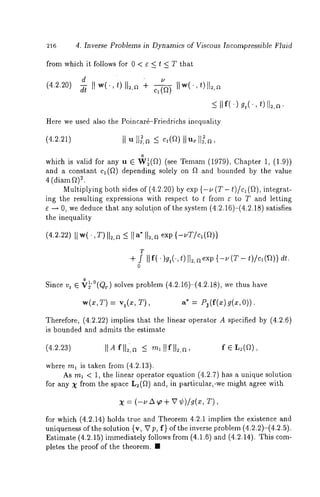
![4.2. Navier-Stokes equations: the final overdetermination 217
To illustrate the results obtained it is worth noting three things.
Remark 4.2.1 Suppose that under the conditions of Theorem 4:2.2 the
function 9 depends only on t under the constraints
g, g’ E C([0, T]), g(t) > O, g’(t) >_ O, g(T) 7~
In this case ml < 1 for any T > 0 and Theorem 4.2.2 turns out to be of
global character. That is to say, the inverse problem (4.2.2)-(4.2.5)
these input data is uniquely solvable for any T, 0 < T < o~.
Remark 4.2.2 If
g = g(t), g, g’ c([0, 7"]), g( T) #
then the inverse problem (4.2.2)-(4.2.5) can be investigated by the method
of separating variables by means of which it is plain to expand its solu-tion
in the Fourier series with respect to the eigenfunctions of the Stokes
operator ~,Pj A. If this happens, the function f is sought in the space
L2(a) assuming that both components Pj f and PGf in the subspaces
2} (t2) and G(a), respectively, are, generally speaking, nontrivial (recall
o
that L~(a) = J (a) ~ G(~)).
Remark 4.2.3 Once the function g depends only on t, it will be possible
to impose the condition of the final overdetermination (4.2.5) omitting the
information about the final value of the pressure gradient V p(x,T). In
other words, the final overdetermination contains v(x, T) = ~o(x) and
o
more. However, in this case we look for the function f in the space J (f~).
In conclusion an example is given as one possible application.
Example 4.2.1 Consider the inverse problem of determining a collection
of functions {v, V p, f}, which satisfy the set of relations
(4.2.24) vt -
(4.2.25) v(x, 0) =
(4.2.26) v(x, t) = (x, t) G St,
(4.2.27) v(x,](https://image.slidesharecdn.com/0824719875inverse-141031173353-conversion-gate01/85/0824719875-inverse-238-320.jpg)
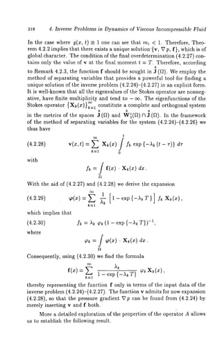
![4.2. Navier-Stokes equations: the final overdetermination 219
Theorem 4.2.3 Let g, gt E C((~ r) and Ig(x,T) > gT> 0 fo r x
Then the operator A is completely continuous on the space L:(~).
Proof We again appeal to the differential properties of the solution w of
problem (4.2.16)-(4.2.18) arguing as in the proof of Theorem 4.2.2.
usual, an arbitrary number v from (0, T) is considered to be fixed. As far
as II w~(., t)tl~,a is continuous on the segment Iv, T], there is v* ~ [v,
such that
(4.2.31)
T
, t) H~,a dt = (T-v)H wx(’,
By means of the element F* = f gt from the space L2(QT) it is straightfor-ward
to verify that the system (4.2.16) implies that
(4.2.32)
With the aid of the equality
T T
it is reasonable to recast (4.2.32)
(4.2.33)
T
From (4.2.31) and (4.2.33) we derive the inequality
(4.2.34)
As stated in Ladyzhenskaya (1970, p. 113]), (4.2.19) implies the estimate
(4.2.35)
T 2
llwxll ,< . II IdItF*(’,t)ll~,~
0](https://image.slidesharecdn.com/0824719875inverse-141031173353-conversion-gate01/85/0824719875-inverse-240-320.jpg)
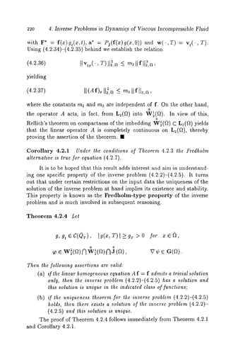
![4.3. Navier-Stokes equations: the integral overdetermination 221
4.3 Nonstationary linearized system of Navier-Stokes equations:
the integral overdetermlnatlon
We are much interested in the inverse problem involving the nonsta-tionary
linearized system of Navier-Stokes equations when the overdeter-ruination
condition is given in a certain integral form.
As in Subsection 4.2 an unknownv ector function of the external force
F1 is sought via the measurement of its indirect indications: the velocity
of the flow v and (or) the pressure gradient Up. In addition, F1 is taken
to be
(4.3.1) F1 = f(t) g(x, t),
where f(t) is unknown, while g(x, t) is given.
With these assumptions, we may set up the inverse problem in which
it is required to find a triple of the functions {v, Vp, f}, which satisfy the
system
(4.3.2) vt-uAv -V p+ f(t ) g(z , t), div v = O, (z , t ) e QT
the initial condition
(4.3.3) v(x, 0) = x E ~2,
the boundary condition
(4.3.4) v (x, t) = (x, t) e St,
and the integral overdetermination condition
(4.3.5) f v(x, t) ¯ w(x) dx = p(t), 0 < t
provided that the functions g, w, p and the coefficient u are known in
advance. We look for a solution of the inverse problem (4.3.2)-(4.3.5)
the class of functions
0 v~ 2W:~0 (Q~~) ~1 J(QT) , Vp ~ G(Q~) , f ~ C([0, T]).
The norm of the space C([0, T])is defined
(4.3.6) [tfllc = sup l exp{-Tt)f(~t)l,
tE[0, T]](https://image.slidesharecdn.com/0824719875inverse-141031173353-conversion-gate01/85/0824719875-inverse-242-320.jpg)
![222 4. Inverse Problems in Dynamics of Viscous Incompressible Fluid
where 7 is a positive number which will be specified below.
In tackling problem (4.3.2)-(4.3.5) one might reasonably try to adapt
the method ascribed to Prilepko and Vksin (1989a). Their methodology
guides the derivation of a linear operator equation of the second kind for f
and necessitates imposing the extra restrictions
g ¯ c([0, r], L2(a)),,o ¯ w~(a)~, ,, ~,’ ¯ C([0,
g(x,t) ¯ w(x) dx[_> go>0 for 0<t <T (go=const).
When an arbitrary function f from C([0, T]) is held fixed, the system
(4.3.2)-(4.3.4) serves as a basis for recovering a pair of the functions {v,
as a solution of the direct problem with the prescribed function g and co-efficient
v. In agreement with Theorem 4.1.2 there exists a unique solution
{v, Vp} of problem (4.3.2)-(4.3.4)
0
Vp¯G(QT),
it being understood that any function f from the space C([0, T]) is asso-ciated
with the unique function v thus obtained. The traditional way of
covering this is to introduce the linear operator
AI: C([O, T]) ~-~ C([O,
acting in accordance with the rule
(4,3.7) (A~ f)(t) = g~(t)
where
g,(t) = / g(z, t) dx
and v is the function involved in the solution {v, V p} of the system (4.3.2)-
(4.3.4), the meaning of which we have discussed above.
Our further step is to consider the linear operator equation of the
second kind over the space C([0, T]):
(4.3.8) f = A, f + h, ’ whereh , = ~9’(,(tt))](https://image.slidesharecdn.com/0824719875inverse-141031173353-conversion-gate01/85/0824719875-inverse-243-320.jpg)
![4.3. Navier-Stokes equations: the integral overdetermination 2:23
Theorem 4.3.1 Let
~, ~’ ~ c([0, T]), ~(0)
~ e w~(~)NoW ~l(ae )oN(~),
Jg(*, O. ~(*) > go> ofor * e [0, T].
Then for a solution of the inverse problem (4.3.2)-(4.3.5) to exist it is
necessary and sufficient thai equation (4.3.8) is solvable.
Proof We first prove the necessity. Let the inverse problem (4.3.2)-(4.3.5)
possess a solution, say {v, Vp, f). Taking the scalar product in L2(~)
between w and both sides of the first equation (4.3.2) we arrive
(4.3.9)
recalling that
0 vp(.,t ). ,.,(~) d. = 0 ~or, .., (~).
From (4.3.9), (4.3.5) and (4.3.7) we conclude that f solves the equation
f= Alf ÷h~.
But this means that (4.3.8) is solvable.
Proceeding to the proof of the sufficiency we suppose that equation
(4.3.8) possesses a solution, say f ~ C([0, T]). By Theorem 4.1.2 on
unique solvability of the direct problem we are able to recover {v,
as the solution of (4.3.2)-(4.3.4) associated with f, so that it remains
show that the function v satisfies the overdetermination condition (4.3.5).
Under the agreement
f ..(:~,t ) ¯ ,,,(:~)d :~= ~,, (t), t e [0,
it is not difficult to check that the initial condition (4.3.3) gives TI(0)
By exactly the same reasoning as in the derivation of (4.3.9) we find that
(4.3.~.o) f = A~ f + ~o’~(t)/g~(t).](https://image.slidesharecdn.com/0824719875inverse-141031173353-conversion-gate01/85/0824719875-inverse-244-320.jpg)
![4. Inverse Problems in Dynamics of Viscous Incompressible Fluid
On the other hand,
(4.3.11) f = A1 f
which is consistent with the initial assumption.
From such reasoning it seems clear that the combination of (4.3.10)
and (4.3.11) gives
~’l(t) = ~’(t)
for t E [0, T]. By the same token,
~,,(o)~ (0) = o,
yielding
~,,(t) = ~(t)
for t E [0, T]. This provides support for the view that {v, 27 p, f} is just a
solution of the inverse problem (4.3.2)-(4.3.5).
In the next theorem we establish sufficient conditions under which the
inverse problem solution can be shown to exist and to be unique.
Theorem 4.3.2 Let
g ~ C([O, T], L~(~))
~, ~a’ e C([0, T]), ~(0) 0,
o 0 ,.o e w~(r~N)W ~(Nr~J ) ( r~),
/g(x, t) .w(x)dx >_ go > O fort ~ [O,
Then there exists a solution of the inverse problem (4.3.2)-(4.3.5), this
solution is unique in the indicated class of functions and the estimates
hold:
(4.3.12) II f IIc- <m Il I ~’I Ic,
(4.3.13) tlvlI~;~)+T1 127P1-1-<= m,%= ll~’llC,
where the constants rnl and ms depend only on the input data of the inverse
problem under consideralion.](https://image.slidesharecdn.com/0824719875inverse-141031173353-conversion-gate01/85/0824719875-inverse-245-320.jpg)
![4.3. Navier-Stokes equations: the integral overdetermination 225
Proof It follows from relation (4.3.7) specifying the operator A1 that
(4.3.14) tlAIIItc< lullA~ll2,a sup (exp{--Tt)
go t E [0, T]
Taking the scalar product in the space L~(~) between v and the first equa-tion
(4.3.2) we establish the relation known as the energy identity:
g. 2 dt IIv(.,OIl~,a÷I~Iv ,(.,t)ll~,~ f(t)
vdx,
which implies the inequality
d
d~ Ilv("t)ll~’~ < Hf(t)g("t)[l~’a’ O<t<T.
Integrating over r from 0 to t the resulting expression yields
(4.3.15) IIv(., 011~,~
t
~<I Iv(., o)112,~s÷u p Ilg(.,t)ll~,a / If(r)[ dr. tE[0,T]
0
Putting these together with the initial condition
timate
(4.3.16)
where
4.3.3) we obtain the es-m3
= --IlzXwll~,~ sup IIg( ,t)ll~,a.
790 tE[0,T]
For the moment, we choose 7 so that
(4.3.17) m3 < 1.
From (4.3.16) and (4.3.17) we deduce that there exists a unique solution
to equation (4.3.8) in C([0, T]) and (4.3.12) holds true. Relations (4.1.6)
and (4.3.12) imply estimate (4.3.13). Due to Theorem 4.3.1 the inverse
problem (4.3.2)-(4.3.5) has a solution {v, Vp, f}. In order to prove
uniqueness, assume to the contrary that there were two distinct collections
{v~, V p~, fa } and {v~, V p~, f~} both solving the inverse problem (4.3.2)-
(4.3.5). We claim that f~ does not coincide with f~, since otherwise v~
and V pa would be equal to v~ and V p~, respectively, due to the unique-ness
theorem for the direct problem related to the system (4.3.2)-(4.3.4).
Repeating the same arguments adopted in the development of (4,3.9) for
these specific cases we see that both functions fa and f~ satisfy (4.3.8). But
this contradicts the solution uniqueness established above for the governing
equation, thereby completing the proof of the theorem. ¯](https://image.slidesharecdn.com/0824719875inverse-141031173353-conversion-gate01/85/0824719875-inverse-246-320.jpg)
![226 4. Inverse Problems in Dynamics of Viscous Incompressible Fluid
In practical applications of advanced theory one could require to mea-sure
the pressure gradient V p instead of the flow velocity v. In that case the
statement of the inverse problem is somewhat different (see Vasin (1992b))
and necessitates seeking a collection of the functions {v, Vp,/), which
satisfy in QT the system
(4.3.18) vt-uAv=-~Tp+f(t) g(x,t), divv=0, (x,t) EQT,
the initial condition
(4.3.19) v(x, 0)=
the boundary condition
(4.3.20) v
and the condition of integral overdeterminafion
(4.3.21) f V p(~, t) ¯ X(x) ¢(t)
provided that the functions g, X, ¢ and the coefficient u are given.
In a commonse tting we look for a solution of (4.3.18)-(4.3.21) in
class of functions
o
v~Wz, 2,1o(QT)~3(Q.T), f~C([O,T]),
under the agreement that the integral
JVp(x, t)~(~)dx
o
is continuous in t E [0, T] for any ¯ ~ G(~) N W~(f~). In addition,
supposes that
Jg(x,t) ¯ X(z)
X ¯ W[(f~), ~b e C([0, T]),
>_ go > 0, 0 < t < T (go = const).](https://image.slidesharecdn.com/0824719875inverse-141031173353-conversion-gate01/85/0824719875-inverse-247-320.jpg)
![4.3. Navier-Stokes equations: the integral overdetermination 227
On the same grounds as in the derivation of (4.3.8), we involve in the
further development the linear operator
A2: C([0, T]) ~ C([0,
acting in accordance with the rule
(4.3.22) (A2 f)(t) - g2(t)_ dx ,
where
f
g2(t) = / g(X, t) dx.
In the theorem below we establish the conditions under which the linear
operator equation of the second kind
(4.3.23) f = A2 f + h~
with h~ = -¢(t)/g2(t) is equivalent to the inverse problem at hand.
Theorem 4.3.3 Let
([ ))
°
g E c 0, T], L2(fl , X e G(fl)NW~(~)(~W~(~),
¢ ~ C([0, T]), g(x,t).x(x)dx _>g0>0, 0<t<T.
Then for a solution of the inverse problem (4.3.18)-(4.3.21) to exist it is
necessary and sufficient that there exists a solution to equation (4.3.23).
Proof We proceed to prove the necessity. Let the inverse problem (4.3.18)-
0
(4.3.21) admit a solution, say {v, ~’p, f}. In dealing with t GJ( Qr) an
X G G(f~) we can show that the system (4.3.18) implies
(4.3.24) /Vp(x, t). X(x) = u / v( x, t). A X(x)dx
+ f(t) g(x, t) ¯ X(~e) dx,](https://image.slidesharecdn.com/0824719875inverse-141031173353-conversion-gate01/85/0824719875-inverse-248-320.jpg)
![228 4. Inverse Problems in Dynamics of Viscous Incompressible Fluid
since
Observe that the function on the left-hand side of (4.3.24 is continuous on
the segment [0, T]. This is due to the fact that
/ (v t v t)) ¯
+ If( t + At)l IIxII2,rt " IIg(’, t + At) - g(., t)lt~,rt
+I Ig (t,) I1¯2I ,Ix~ I I~l,f~(+ t/ ~-t ,f)( t)l
where f e C([0, T]) and
With relation (4.3.22) in view, which specifies the operator A2,
deduce that (4.3.24) yields f = A2 f + h~. This proves the necessity.
The sufficiency can be established in a similar way as in the proof
of Theorem 4.3.1 and the details are omitted here. Thus, the theorem is
completely proved. ¯
Theorem 4.3.4 Let
g G C([O, T], L~(~))
o
¢ e c([0, T]), g(x, t) . x(x) _>g0>0,
Then there exists a solution of the inverse problem (4.3.18)-(4.3.21), this
solution is unique in the indicated class of functions and the estimates hold:
(4.3.25) II f IIc_ <,~ 4II ¢I Ic,
(4.3.26)
where m~ and m~ are the constants depending only on the inpul data of the
inverse problem under consideration.](https://image.slidesharecdn.com/0824719875inverse-141031173353-conversion-gate01/85/0824719875-inverse-249-320.jpg)
![4.3. Navier-Stokes equations: the integral overdetermination 229
Proof We rely on the estimate for the operator A2 specified by (4.3.22):
(4.3.27) (A~f)(t) <_ llAx ll=,n . ii v(.,t)ll~,~.
go
Relations (4.3.16) and (4.3.27) together imply the inequality
(4.3.2S) [[A2 f [[c -< m~[ [ f[[c,
where
--IIX xll, sup IIg(,OIl ,s
7 go t E [0, T]
Arguing as in the proof of Theorem 4.3.2 we conclude that the in-verse
problem (4.3.18)-(4.3.21) has a solution and this solution is unique.
Estimate (4.3.26) follows from (4.1.4) and (4.3.25).
It is worth noting here that the results set forth in this section can
easily be generalized for the linearized Navier-Stokes equations of rather
general form where the system (4.3.2) will be replaced
(4.3.:29)
vt- t, Av+ ~ B~(x,t)vx~ +A(x,t)v = -Vp+f(t) g(z,t),
k=l
div v = O, (x, t) e QT
where Bk and A are given (n x n)-matrices with entries b~j and aij , re-spectively.
Once again, the initial and boundary conditions as well as the
overdetermination condition are prescribed by (4.3.3)-(4.3.5). As an
ample we cite here the theorem proved by Vasin (1992a).
Theorem 4.3.5 Let bf, aij ¯ C([0, T],L4(f2)), bij ¯ J(Qr), oJ
o o
W~(~) [~1 w~l(~-~) N J (~), ¢/~ ¯ el(J0, ~o(0)= 0, g¯ C([0,T]
and let the inequality
/ g(x,t)w(x) > go >0 (go :const), 0<t <T,
hold. Then a solution
v¯ W~2,, o1~ ){ {-1 ~ ](Q~), Vp ¯ G(Q~), f¯C([O,T])](https://image.slidesharecdn.com/0824719875inverse-141031173353-conversion-gate01/85/0824719875-inverse-250-320.jpg)
![23o 4. Inverse Problems in Dynamics of Viscous Incompressible Fluid
of the inverse problem (4.3.29), (4.3.3)-(4.3.5) exists, is unique and has
A similar result is still valid in the case where the overdetermination
condition is of the form (4.3.21). Here ij ref ers to thevector with com-ponents
b~j (k = 1,2 or k = 1,2,3). The symbol:~(Qr) stands for
subspace of L2(Qr) consisting of all vector functions belonging to J(ft)
almost all t ¯ [0, T]. The space J(f~) contains the L2(f~)-vectors being
o
orthogonal to all vectors like V¢ for ¢ ¯ W~(f~).
4.4 Nonstationary nonlinear system of Navier-Stokes equations:
three-dimensional flow
We begin by placing the statement of the inverse problem for the system
(4.1.8) assuming that the vector function F~ involved in (4.1.8) i~ repre-sentable
by
F2 = f(x) g(x, t),
where g(x, t) is a given scalar function and f(x) is an unknown vector
function.
The inverse problem here is to find a triple of the vector functions
{v, Vp, f}, which satisfy in Qr the nonstationary nonlinear Navier-
Stokes system
vt - ~’Av + (v, V)v = -Vp+ f(x) g(x, t),
(4.4.1)
div v = 0, (x, t) ¯ QT
the initial condition
(4.4.2) v (x, 0) = a(x), x ¯
the boundary condition
(4.4.3) v (x, t) = (x, t) ¯ ST,
and the final overdetermination conditions
(4.4.4) v(x, T) = ~p(x), Vp(x, T) = V¢(x), x ¯
provided that the functions a, ~o, V ¢, g and the coefficient u are given. By
a solution of the inverse problem (4.4.1)-(4.4.4) we mean a triple {v, Vp,
such that
0
v ¯ W22,1,o(QT) NJ (Qr) , f ¯ L2(a),](https://image.slidesharecdn.com/0824719875inverse-141031173353-conversion-gate01/85/0824719875-inverse-251-320.jpg)
![4.4. Navier-Stokes equations: three-dimensional flow 231
for any t E [0, T] and it continuously depends on t in the L2(f~)-norm
on the segment [0, T] and, in addition, all of the relations (4.4.1)-(4.4.4)
occur.
Throughout Section 4.4, we will assume that the dilnension of the
vt
domain of spatial variables f~ is equal to 3, that is, f~ C Ra. First, we
are going to derive some stability estimates for the solutions of the system
(4.1.8)-(4.1.10). Let v’ = v’(z, t) v" =v"( z, t) be thesol utio ns of
the system (4.1.8)-(4.1.10) corresponding to the initial velocities a~, a~’
the external forces F~, F~’, respectively. The function v~ is subject to the
integral identity
i v~~ ¯ / = F~ ,. ¯ dx,
o o
where ¢ is an arbitrary function from the space W~(~) ~ 3 (~).
A similar relation remains valid with regard to the function v". There-fore,
by subtracting the first identity fi’om the second we deduce that
(4.4.5) J(v’-v’)t.~dx+~J(v’-v")~.~ dx
+/(¢, v)(¢- ¢’) dz
+ f (v’-v", V) O dz
o o
Since v’(., t) and v"(., t) both are located in Wg(a) ~ J (a), it is mean-ingful
to substitute ~ = v~ - v" into (4.4.5). The outcome of this
1 d "
(4.4.6)
With the aid of the relation
(v’, v)(v’- v")¯ (v’ - v")](https://image.slidesharecdn.com/0824719875inverse-141031173353-conversion-gate01/85/0824719875-inverse-252-320.jpg)
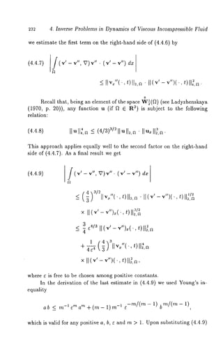
![234 4. Inverse Problems in Dynamics of Viscous Incompressible Fluid
All this enables us to explore the inverse problem (4.4.1)-(4.4.4)
deeply by means of a subset D C L2(fl) such that
D= {f ~ L2(f2): []f[[2,~ -< i’
In the sequel we will always assume that a and 9~ belong to W~(f~)
o o
W~(f~) n 3 (f~) and
and
(4.4.14)
where
Ig(~, T)I _> g~ > 0 for x ~ ~ (gT ~" const),
ml m2 < u3 (4/32)-1,
/3 = (4/3) 3/4 ,(1c/,4(ft))
-~= II~’zx--(a,V)-ILa+ sup I~(:~,t)l
T
+ supI g(x,0 )1+ / supI g,(~,t )l dt
x~t x~gt
0
and cl (~) is the constant from the Poincarfi-Friedrjchs inequality (4.2.21).
The system (4.4.1)-(4.4.3) with f ~ D can be viewed as a system
the type (4.1.8)-(4.1.10). It is clear that for any f lying within D either
of the functions F2 = fg and (F2)t = fgt belongs to the space L2(f~.).
Granted (4.4.14), the function F2 = fg satisfies condition (4.1.11) for
f from D. Consequently, by Theorem 4.1.4 one can find a unique pair of
the functions {v, Vp} as a solution of the direct problem (4.4.1)-(4.4.3)](https://image.slidesharecdn.com/0824719875inverse-141031173353-conversion-gate01/85/0824719875-inverse-255-320.jpg)
![4.4. Navier-Stokes equations: three-dimensionM flow 235
corresponding to a suitably chosen function f E D. In the framework of
Theorems 4.1.4-4.1.5 we refer to the nonlinear operator
A: D H L~(V~)
acting in accordance with the rule
(Af) (x) = , T), x E f~
where v is the function entering the set {v, Vp} and solving the direct
problem (4.4.1)-(4.4.3).
One more nonlinear operator
B: D ~
1
(B f)(x) g(x, 73 (Af) (x), .x ~ ~,
with the values
(4.4.15)
complementsc areful analysis of the nonlinear operator equation of the sec-ond
kind for f:
(4.4.16) f = /3 f +
where
1 [-u A ~o + (~o, V)+V~b] x = g(z, T) ~ "
Theorem 4.4.1 Let
aCRa, g,gt~C(Qr), Ig(z,T)I~>0 for x~,
0 0
If (4.4.14) holds, then the operator B is completely continuous on D.
Proof The theorem will be proved if we succeed in showing that the op-erator
A is completely continuous on D. Choosing f in D arbitrarily we
consider a sequence {f ~}~=t of elements f~ ~ D such that
Let {v~, Vp~} be the solution of the direct problem (4.4.1)-(4.4.3)
corresponding to the external force function f~ g and the initial velocity a](https://image.slidesharecdn.com/0824719875inverse-141031173353-conversion-gate01/85/0824719875-inverse-256-320.jpg)
![4. Inverse Problems in Dynamics of Viscous Incompressible Fluid
and let (v, V p) be the solution of the same problem corresponding to the
external force function fg and the initial velocity a. Then the functions
v~ - v and V(p~ - p) satisfy the system
(4.4.17)
(4.4.18)
(4.4.19)
where
( v~- v)~- ~z x( ,,k -
= -V(p~ -p) ÷ F~, div(v~ - v) ---
(v~ - v) (~, o) = o, ~,
(vk - v) (x, t) = 0, (x,
F~ = (f~ -f)g+ (v~, V)(v-v~)+ (v-v~,
We note in passing that the norm of F~ can be estimated as follows:
+ II (v- v~, V)v
The Cauchy-Schwarz inequality is involved in the estimation of the second
and third terms on the right-hand side of (4.4.20). The same procedure
works with a great success in establishing the relations
(4.4.21) I] (v~, v)(v - vk)II=,QT
T
0 ~
_< { sup [sup
re[O, T]
and
(4.4.22)
_< 3 II(v~ v-) ( " , IIt)~ ,a~ IIv~(,OIl~,~~ dt
0](https://image.slidesharecdn.com/0824719875inverse-141031173353-conversion-gate01/85/0824719875-inverse-257-320.jpg)
![4.4. Navier-Stokes equations: three-dimensional flow 237
The estimation of the first factor on the right-hand side of (4.4.21) can
be done using (4.1.15) and the theorem of embedding W~(f~)
(see Ladyzhenskaya et al. (1968, p. 78)), due to which we thus
(4.4.23) II (v~,v ) (v - v,~)I I,,, ~ ~<c *M s(f~II) (v - v,~)~
where
-- 11/2~
× 1 +c*[.~.(f~:)(~(fl:)+ M3(f,~))]
+ c" [~~_ (fk)(~’~ (ft,)+ M3 (ft,))]
T
Ml(fk=) Ilall~,~+llf~ll~,~ supI g(x,t ) l dr,
x(~Ft
0
M~(f~=) I I~Aa(-a , V)all~,~÷ IIf~I 1~,~s upI g(~,
T
÷ IIf~I 1~,~/ sup
0
M~(f~=) IIf~ll~,~ s~pI g(z, t)l.
(~,t)~%
The symbol c* denotes the constant depending on T, f~ and v. In what
follows the same symbol c* will stand for different constants. It is to be
hoped that this should~ cause~no confusion.~ It is str~aightforward to verify
that the values of Ms(f~), Ml(fk), M~(f~) and Ma(f~) are bounded
k --~ oo, since the sequence {f~)~=l converges to f in the L2(a)-norm.
By (4.1.15), (4.2.21) and the theorem of embedding from W~(f~)
L4(f~) (~2 C R3), we see that (4.4.22) implies the estimate
(4.4.24) II(v-v~,](https://image.slidesharecdn.com/0824719875inverse-141031173353-conversion-gate01/85/0824719875-inverse-258-320.jpg)
![238 4. Inverse Problems in Dynamics of Viscous Incompressible Fluid
T
o
T
where
-31J-2e}" []~l(f)(lW/2(f)-J-J/Z3(f))]
T
M~(f=) Ilall.,~+ Ilfll~,~/ sup1 9(’~~, )
o
dt
M2(f=) II~’Aa-(aV, )all.,n+I lfll~,n supg (~,
T
+ Ilfll2,a J sup
o
I gt(xt,) dt,
M3(f) Il fll2,a su p 19 (x,
Substituting (4.4.23) and (4.4.24)into (4.4.20)
(4.4.25)
T
o
IIf~- fll2,a
+ c* (M-~5(f~) + Ms(f)) (v - v ~). I1., Q~.](https://image.slidesharecdn.com/0824719875inverse-141031173353-conversion-gate01/85/0824719875-inverse-259-320.jpg)
![4.4. Navier-Stokes equations: three-dimensional flow 239
We now apply the stability estimates (4.4.12)-(4.4.13) with F~ =
and F = f g standing in place of the functions F~ and F~I, respectively, thus
causing v’ = vk, v" = v and a2 = a2 = a. With these relations in view,
(4.4.12) implies that
2
(4.4.26) II(v~-v)(’,~)ll2,a~exp
T
and (4.4.13) is followed
T
sup Ig(x, r)[ d~-1 Ilfk -fll2,a
(4.4.27) II(v~ v)~
4 sup IIv~(’,~)ll~,~
-- I]2’QT ~ ~ t(~[0,T]
×llv~-vll~,~÷ sup Ig(~,z)l
(~,t)e%
× IIf~- fl12,~:r ~/~I Iv~
If one squares both sides of (4.4.26) and integrates the resulting expressions
over t from 0 to T, then
T
(4.4.28) IIv~-~l12,~ ~r exp ~ IIv~(.,~)ll~,ad~
0
T 2
Since the sequence {fk}~=l converges to f in the L2(f~)-norm, inequality
(4.4.28) implies the convergence
(4.4.29) II v~- v tl2,~ T-- -~0 , ~ ~ ~,
which in combination with (4.4.27) gives
(4.4.30) I1( v~ - v)~ 112, ~T -~ ~ -~ ~.
By successively applying (4.4.28), (4.4.30) and (4.4.25) we arrive
limit relation](https://image.slidesharecdn.com/0824719875inverse-141031173353-conversion-gate01/85/0824719875-inverse-260-320.jpg)
![4.4. Navier-Stokes equations: three-dimensional flow 241
where the explicit formulae for Ms(fk) and Ms(f) are given by (4.4.23)
(4.4.24), respectively.
In the case where fk 6 D, the norm of (v~)t, can be estimated with
the aid of (4.1.14) as follows:
(4.4.35) [u-~(v-lmlm2) 1/2] II(v~)txll~,QT
_<I~ 1~’A ~-(aV, )all~,~+ IIf~I 1~,~[ supb (~,0 )1]
(a,V)all~, a+Hf~[[~,a sup [g(x,O)
sup I~t(~,¢)l d~
where ml, m2 and /~ have been introduced in (4.4.14). From such manip-ulations
it seems clear that the first factor on the left-hand side of (4.4.35)
does not depend on k and is strictly positive by virtue of (4.4.14). More-over,
estimate (4.4.35) implies that the norm II (v~)tx I1~, Q~ is bounded
k ~ 0. With this in mind, we conclude on the basis of estimate (4.4.34)
that the norm II (Fk)t 112,QT is also bounded as k ~
Being concerned with F~ and (F~ h from the space L2(Q~) we can
treat the system (4.4.17)-(4.4.19) as a system of the type (4.1.3)-(4.1.5).
Just for this reason all the assertions of Theorem 4.2.2 remain valid when
expression (4.2.19) is considered in terms of the solutions of (4.4.17)-
(4.4.19):
(4.4.36) v~- vh( ., t)113,~+ ~ II (v~- v)¢~( ., t)II~,rOdt
O<e<T.
Relation (4.4.36) implies that
T
T
_</ H(F/~)t(’, t)[l~,a’ tt(v~-v)~(.,t)]]~,adt, O<~_<T,](https://image.slidesharecdn.com/0824719875inverse-141031173353-conversion-gate01/85/0824719875-inverse-262-320.jpg)
![242 4. Inverse Problems in Dynamics of Viscous Incompressible Fluid
yielding
1
1 + ~ II(v~ -v),(.,
Becauslte( vk- vh(,t )II=,~i s continuouons the segment [0, T], we
are able to pass in the preceding inequality to the limit as ¢ ~ 0 and, as a
f(i4n.a4l. 37re) sult[,~ (vg~et- vt)ht(e’ ,Tes)tUim~,aat5e~](Fk)tU:,Q ~ ¯ [~ (v~ - v)t ~,O~
assuming that the boundary condition (4.4.18) is homogeneous.
As stated above, the norm ~ (F~)t U:, Qv is bounded ~ k ~ ~. Ap-plying
estimate (4.4.37), relation (4.4.32) and the definition of the operator
A we establish
This provides support for the view that the nonlinear operator A is con-tinuous
on D.
Let us show that any bounded subset of the-~et D is carried by the
operator A into ~ set being compact in the space L~(~). To that end,
rewrite the system (4.4.1)-(4.4.3)
(4.4.38) vt-u~v=-Vp+F~, divv=0, (z,t) GQ~,
(4.4.39) v(x, 0)=a(x), xE~, v(x,t)=0, (x,t)
where
~1 = f(x) g(x, t) - (v,
As in the derivation of (4.4.25) and (4.4.34) we make use of the esti-mates
+ c* M~(f)vI~II I~,
(4.4.40)
sup Ig~(:~, t)l ~ dt Ilfl12,~
+ c*M ~(f)vII~1 12,Q ~,](https://image.slidesharecdn.com/0824719875inverse-141031173353-conversion-gate01/85/0824719875-inverse-263-320.jpg)
![4.4. Navier-Stokes equations: three-dimensionM flow 243
where Ms(f) has been introduced in (4.4.24).
Further treatment of (4.4.38)-(4.4.39) as a system of the type (4.1.3)-
(4.1.4) with reference to the proof of Theorem 4.2.3 permits us to deduce,
keeping vt(., T) E ~¢~(f~) R ~ (~) and holding e from the interval
fixed, that (4.2.34) yields
(4.4.41) IIv~(’’ ~)ll~,-~ ~III(F~)~II~,~÷ ~ 1(T- e)
23 T
]
x [[ u Aa - (a, ~) a + F(., O)[[~, a + T [I (Fz)t QT "
Finally, we get from (4.1.14), (4.4.40) and (4.4.41) the estimate for
nonlinear operator A
(4.4.42) II(Af).llg,~<2 [1_+ = ]
- u 2u(T-¢)
"x 1+ u3--~----~x/~Tj
3c* M~(f)~ 2 ]
+llfll~,8 sup I~(~, o)12).
Let an arbitrary bounded subset D1 of the set D be given. Recall
that
D = {f E L~(~): llflt~,a _<
is referred to as the range of the operator A.
Estimate (4.4.42) implies that the nonlinear operator A acts from
o
D C L~(~) into W~(f~) and maps D~ into a certain set /)~ being bounded
in the space W~(~).](https://image.slidesharecdn.com/0824719875inverse-141031173353-conversion-gate01/85/0824719875-inverse-264-320.jpg)
![246 4. Inverse Problems in Dynamics of Viscous Incompressible Fluid
and relations (4.4.14) and (4.4.43) occur. One assumes, in addition, that
the estimate
(4.4.48)
is valid with
m~---[i,n=f ca[g(x,T)[]-~([ ll~Aa- (a, V)a ll~,n
+supgx(~x ’O )Ie xp- 2 c1LtT(~]*]~)
sup [gt(x, t) l exp - dt x~ 2 cl (~)
and
x = g(x,1 T[)-UAcp+(~,V) ~ +V¢] ¯
Then there exists a solution of the inverse problem (4.4.1)-(4.4.4).
Proof We proceed to derive an a priori estimate for the nonlinear operator
B on D. The energy identity (see Ladyzhenskaya (1970) p. 184) suits
perfectly after rewriting it in terms of (4.4.1):
ld
(4.4.49) , t)I Ig~, + ~ ’I Iv ,=(t.,) IIg,
=-f(v,, V)v .v, dx +/(fg,). v,
We are led by evaluating the first term on the right-hand side of (4.4.49)
with the aid of (4.2.21) and (4.4.8)
(4.4.50) (v,, x7)v.v , d~] _<I lv,(., t) 112,¯~ t lv=(.,t ) 112,~
_<( 4/3~)/4c ~/~(~~)I,~I (-t,) lig,~
× II v~(.,t )II~,~.](https://image.slidesharecdn.com/0824719875inverse-141031173353-conversion-gate01/85/0824719875-inverse-267-320.jpg)
![248 4, Inverse Problems in Dynamics of Viscous Incompressible Fluid
Because of (4.4.48), the operator B1 admits the estimate
and, consequently, maps the set D onto itself.
Theorem 4.4.1 implies that B1 is completely continuous on D C
L~(f~). In conformity with Schauder’s fixed-point principle, valid for non-linear
operators, equation (4.4.52) has a solution lying within D. Hence
there exists a solution to equation (4.4.16) and this solution also belongs
D. Finally, by Theorem 4.4.2 we deduce that there exists a solution of the
inverse problem (4.4.1)-(4.4.4), thereby justifying the desired assertion.
As pos£ible illustrations we give several remarks.
Remark 4.4.1 Let in the conditions of Theorem 4.4.3 a = 0 and the
function g will be independent of x. If g E C1([0, T]), g(t) >_ O, g’(t) > 0
and g(T) ¢ O, then inequality (4.4.14) is valid as long
2g~(T) -<1 .ua(4/3~)
Note that ra~ < 1 for any T, 0 < T < cx~. We Choose the functions ~ and
V ¢ so as to satisfy (4.4.43) and provide the validity of the estimate
II -uzx o+ 5 (1- m3) a(T).
Then there exists a solution of the inverse problem (4.4.1)-(4.4.4)
these input data and the final moment t = T with the bounds
0 < T < u3 8
Remark 4.4.2 In the study of the inverse problem (4.4.1)-(4.4.4) we
follow proper guidelines of Remark 4.2.1. The relevant results are available
in Prilepko and Vasin (1991).
4.5 Nonstaionary nonlinear system of Navier-Stokes equations:
two-dimensional flow
We now focus the reader’s attention on the inverse problem (4.4.1)-(4.4.4)
when the fluid flow is plane-parallel, that is, f~ C R~. The main feature of
the two-dimensional case is that Theorem 4.1.6 on solvability of the corre-sponding
nonlinear direct problem (4.1.8)-(4.1.10) is of global character](https://image.slidesharecdn.com/0824719875inverse-141031173353-conversion-gate01/85/0824719875-inverse-269-320.jpg)
![4.5. Navier-Stokes equations: two-dimensionM flow 249
contrast to Theorem 4.1.4 with regard to fl C R3. The basic trends and
tools of research rely essentially on the arguments similar to those adopted
earlier in the three-dimensionM case.
Let us derive a nonlinear operator equation associated with the func-tion
f. Holding f from the space L2(S~) fixed and arguing as in Section 4.4,
we refer to the nonlinear operator
B: L2(~) ~ L2(~)
with the values
1
(4.5.1) (B f)(x) vt(x , T),
T)
where the function v is determined as a unique generalized solution of
the direct problem (4.4.1)-(4.4.3), which exists and possesses the required
smoothness in accordance with Theorems 4.1.6 and 4.1.7, respectively.
Unlike the three-dimensional case the nonlinear operator B is usually
defined on the entire space L2(f~).
Consider the nonlinear equation of the second kind for the function f
over the space L2(~):
(4.5.2) f = B f + x,
where
x - g(.,1 T[-)uA~+ (~, V)~o+ V¢]
Theorem 4.5.1 Let
aeR2, g,~,cc(O~), I~(~,r)l>~>0 fo~ ~efi,
Then the nonlinear operator B is completely continuous on the space L~(f~).
Arguinga s in the proof of Theorem4 .4.1 we can arrive at the assertion
of the theorem. Mores pecifically, in this case the norms II vd., 0112a, and
live(’, t)l12,~ should be majorized with the aid of (4.1.18) and (4.1.17)
rather than of (4.1.13) and (4.1.12) (for more detail see Prilepko and
(1989b)).](https://image.slidesharecdn.com/0824719875inverse-141031173353-conversion-gate01/85/0824719875-inverse-270-320.jpg)
![25O
Theorem 4.5.2 Let
2~,CR
and let
4. Inverse Problems in Dynamics of Viscous Incompressible Fluid
~,g~C(~), ig(~,T)l>9~>o for
o o
~,~ ~ w~(~f)~ w ~(~f)~ J (~), ~ ~
(4.5.3) 11~’11~,~2 c,(~) <.,
]1/4
where cl(f~) is the constant from (4.2.21). If equation (4.5.2) is solvable,
then so is the inverse problem (4.4.1)-(4.4.4).
Proof In establishing this result we approve the scheme of proving Theorem
4.4.2 with minor changes. In particular, (4.4.46) should be estimated
follows:
_< ~c~(~)1 l~’ll4,~ I1~1*1~,2~
] 1/4
o
This is due to the fact that any function u 6 W~(Q), f~ C 2, i s s ubject
to the relation
(4.5.4)
Theorem 4.5.3 Let
~CR~, g,g,~C(Q~), Ig(x,T)l>_g~>O for
o o
a, ~o 6 W~(fl) nw~(~) n a
and let estimate (4.5.3) be true. If
(4.5.5) rn6= m~+ II X1 12,~< 1,](https://image.slidesharecdn.com/0824719875inverse-141031173353-conversion-gate01/85/0824719875-inverse-271-320.jpg)
![4. Inverse Problems in Dynamics of ViscoUs Incompressible Fluid
In rearranging the right-hand side of (4.5.7) we need the inequality
22,ab < 6a2+6-1b
which is valid for arbitrary 6 > 0 and yields
We substitute (4.~.8) with 6 = u/~ into (4.~.7) and take into account
(4.2.21). As a final result we get
d
1
Multiplying both sides of (4.5.9) by exp [- ~2q(n) ] and introducing
new %nctions
o~(~=) 1 fly,(, *)ll~,a,
ct~(t) = exp
one can rewrite (4.5.9)
dy(t)
(4.5.10)
dt
. (T - t) /
~c~(~J) llf(.
~,(’, t) ll~,a,
oh(t) y(t) q- o~(t)
It is easily seen that (4.5.10) satisfies Gronwall’s lemma. In the pre-ceding
notations,
(4.5.11) ]]vt(. ,t) ll~,n_<exp [~ ]]v~ll~,Qr]
x IIv,(,, O)G,ne xp2 cl(a)
’ [
0](https://image.slidesharecdn.com/0824719875inverse-141031173353-conversion-gate01/85/0824719875-inverse-273-320.jpg)
![4.5. Navier-Stokes equations: two-dimensional flow 253
Because of (4.1.17), inequality (4.5.11) assures us of the validity of
estimate
(4.5.12)l]vt(.,T)[[~,~- ~_<ex{p 71 ]la[]]~’a
+ ~a ~easup [g(x, t)[ dt II fll~,a
+sup 19(*, 0)111f ll~, a] exp[
~’T
¯ ~a 2 c~( ~)
T
/8uplgt(x’t)lexp p(T-t)x~a
2c1(f~)
o
Relation (4.5.12) serves to motivate that the nonlinear operator B specified
by (4.5.1) admits the estimate
(4.5.13) lIBf ll~,a_<m ~, f~D,
where
D = { f e L~(f2): Ilfll~,a _< 1 }.
We refer to the nonlinear operator
with the values
(4.5.14) B1 f = B f + X,
where
x - g(~, ~) ~, .
Theorem 4.5.1 guarantees that the operator B is completely continuous on
L~(V/). Then so is the operator B1 on L:(~). From (4.5.5) and (4.5.13)
follows that
(4.5.15) [1 B~f ll~,a_ <m ~÷ II x I1~,~= m~< 1](https://image.slidesharecdn.com/0824719875inverse-141031173353-conversion-gate01/85/0824719875-inverse-274-320.jpg)
![254 4. Inverse Problems in Dynamics of Viscous Incompressible Fluid
for arbitrary f E D.
This provides enough reason to conclude that the nonlinear operator
B1 is completely continuous and carries the closed bounded set D into
itself. Schauder’s fixed-point principle implies that B1 has a fixed point
lying within D. In the language of operator equations, this means that the
equation
(4.5.16) f = B1 f
possesses a solution and this solution belongs to D. True, it is to be shown
that the same remains valid for equation (4.5.2). Then Theorem 4.5.2 yields
that there exists a solution of the inverse problem (4.4.1)-(4:4.4), thereby
completing the proof of the theorem. ¯
Remark 4.5.1 Of special interest is one possible application to a =
0 and g(x,t) = 1. In that case ml < 1 for any T from the interval
(0, -3/[3 c~(f~)]). The functions ~o and V ¢can be so chosen as to satisfy
(4.5.3) and the inequality
thereby providing the validity of estimate (4.5.5). Therefore, Theorem 4.5.3
yields that there exists a solution of the inverse problem (4.4.1)-(4.4.4)
these input data once we take the final moment t = T from the interval
( 0, ~3/[8 el(a)]).
4.6 Nonstationary nonlinear system of Navier-Stokes equations:
the integral overdetermination
Given a bounded domain Ft in the plane R2 2w,ith boundary 0~ of class C
the system consisting of the nonstationary nonlinear Navier-$tokes
equations and the ineompressibility equation
(4.6.1)
divv = O,
will be of special investigations for (z, t)
provided that the vector external force function F is representable by
(4.6.2) F = f(t) g(x,t),](https://image.slidesharecdn.com/0824719875inverse-141031173353-conversion-gate01/85/0824719875-inverse-275-320.jpg)
![4.6. Navier-Stokes equations: the integral overdetermination 255
where the vector g is known in advance, while the unknown scalar coeffi-cient
f is sought.
The nonlinear inverse problem consists of finding a set of the functions
{v, Vp, f}, which satisfy the system (4.6.1)=(4.6.2) and the function
involved complies also with the initial condition
(4.6.3) v(x, 0) = a(x), x ¯ a,
the boundary condition
(4.6.4) v(x, t) = (x, t) ¯ r =cqf~ x [0, T] ,
and the condition of integral overdetermination
(4.6.5) f v(x,t) . co(x) dx = ~(t), 0 < t <T,
when operating with the functions g, w, a, ~ and the coefficient ~,.
Definition 4.6.1 A pair of the functions {v, f} is said to be a weak
generalized solution of the nonlinear inverse problem concerned if
,, ¯ c([0,T ]0;J (a))NL 2([o, 0 0
v(x,t) ¯ ,~(x) dx ¯ W~(0, T), ’v’,I’ 4¢~(a)N]) ( ;~ ¯ L2(o, T),
0 0
and they satisfy for any ~ ¯ W~(~) V~ 3 (~) the integral identity
(4.6.6) d f v(x, t) ¯ V(~) d-~
+ ~ / v.(.,t) ¯ ¢~(.)
+ / (~(~t, ), v)~(~t,) ¯ e(x)
= f f(t)g(a:,t) . ~(z)](https://image.slidesharecdn.com/0824719875inverse-141031173353-conversion-gate01/85/0824719875-inverse-276-320.jpg)
![256 4. Inverse Problems in Dynamics of Viscous Incompressible Fluid
along with the initial condition (4.6.3) and the overdetermination condition
(4.6.5).
It is worth emphasizing here the incompressibility of the fluid and
the boundary condition (4.6.4) are taken into account in Definition 4.6.1
o o
in the sense that the function v(., t) belongs to the space W~(f])
for almost all t ¯ [0, T].
Later discussions of the inverse problem at hand are based on the
paper by Vasin (1993). In the sequel we will assume that the domain ~
space variables is plane and the input data functions meet the requirements
o o o ¯ J(a), g ¯ C([0, T], L2(~)) ¯ w (a) w (a) (a),
~,¯W~(0, T), /g(x,t) ¯ w(x) dx >_go >0, O<t<T (go =-const).
With these assumptions, we proceed to derive an operator equ.ation
of the second kind for the scalar function f. This amounts to holding
an arbitrary function f from the space L2(0, T) fixed and substituting
into the system (4.6.1) and identity (4.6.6) both. Combination of identity
(4.6.6) written above and the initial condition (4.6.3) constitutes what
called a weak statement of the direct problem (4.6.1)-(4.6.4) of finding
function v.
0
Since F = fg ¯ L2(Qr), a ¯ J(~) and ~ 2, ther e exis ts a un iq ue
function v satisfying identity (4.6.6) with the coefficient f fixed and the
initial condition (4.6.3). In every such case the function v should belong
to the desired spaces of functions (see Temam(1 979)) and any function
from the space L2(0, T) can uniquely be put in correspondence with the
vector function
o 0 o
v ¯ C ([0, T]; J (Ft)) f~ L2 ([0, T]; W~(Q)g~
The traditional way of covering this is to refer to the nonlinear operator
A: L2(O, T) ~ L~(O,
acting in accordance with the rule](https://image.slidesharecdn.com/0824719875inverse-141031173353-conversion-gate01/85/0824719875-inverse-277-320.jpg)
![4.6. Navier-Stokes equations: the integral overdetermination 257
where v has been already found as a weak solution of the system (4.6.1)-
(4.6.4) and
gl(t) / g(x,t) ¯ w(x)
We proceed to study the operator equation of the second kind over the
space L~([O, T]):
(4.6.8) f = Af.
An interrelation between the inverse problem (4.6.1)-(4.6.5) and the
linear equation (4.6.8) from the viewpoint of their solvability is revealed
the following assertion.
0
Theorem 4.6.1 Let ~ C R2, g ¯ C([0, T], L2(~)), a ¯ J(~),
,,., ¯ w~(an) ~ ’(r~n) J (r~)¯ w~’ (oT, ),
(4.6.9)
g(z, t) ¯ co(zd)z >_ 90 > 0 < t < T.
Then the following assertions are valid:
(a) if the inverse problem (4.6.11-(4.6.51 is solvable, then so is equation
(4.6.8);
(b) if equation (4.6.8) has a solution and the compatibility condition
/~(~¯ .),(~d)z = ~(o)
holds, then there exists a solution of the inverse problem (4.6.11-
(4.6.5).
Proof We proceed to prove item (a). Let the inverse problem (4.6.1)-
(4.6.5) have a solution, say {v, f). By Definition 4.6.1 the pair {v,
satisfies (4.6.6) with any ¢ from W~(~) R ~¢~(~) R J (~). By
setting ,~(x) co(x) weobtain
d /v(x,t).w(x)dx+u /vx(z,t).w~(x)dx
(4’6’10/
+ / (v(x,t),V)v(x,t) ¯ co(x) dx = f(t)](https://image.slidesharecdn.com/0824719875inverse-141031173353-conversion-gate01/85/0824719875-inverse-278-320.jpg)
![4.6. Navier-Stokes equations: the integral overdetermination 259
If, with the compatibility condition (4.6.9 1 in view, one integrates the pre-ceding
relation from 0 to t, then from the resulting expression, it seems clear
that the function v does follow the integral overdetermination (4.6.5). Be-cause
of this, the collection {v, f} is just a weak solution of the inverse
problem (4.6.1)-(4.6.5) and this proves the assertion of the theorem.
We should raise the question of the solvability of the inverse problem
(4.6.1)-(4.6.5). For this, we have occasion to use a closed ball O in
space L2(O, T) with center 9’/91 such that
(4.6.13) 73= { f e L2(O, T): Il f - p’/gl ll2,(O,T) <_ r
where
g~(t) = / g(x,t) - w(x) dx.
In what follows the symbol A~ will stand for the kth degree of the operator
Afor k6N.
0
Theorem 4.6.2 Let
o o
w ¯ W~(a) fflW~(a) VI J (a), x ¯ L~(Q), ~ ¯ W~(O, T)and
g(x,t) ¯ w(x) dx > go >0 (go---const), 0<t <T.
One assumes, in additidn, that the nonlinear operator A carries the ball 73
i~nto itself. Then there exists a positive integer k such that the operator A
is a contraction mapping in the ball 73.
Proof Let either of the functions f~ and f~ belong to the ball 73. By the
definition of the operator A,
t
(4.6.14) II A f~ - A f~ lie, (0,,)
0
t
v )x.
-~- (v2, V)(v dx 2 1 -- V2) ¯ 03(~)]](https://image.slidesharecdn.com/0824719875inverse-141031173353-conversion-gate01/85/0824719875-inverse-280-320.jpg)
![260 4. Inverse Problems in Dynamics of Viscous Incompressible Fluid
where the functions vl and v~ are associated with the coefficients fl and
f~, respectively.
The absolute value on the right-hand side of (4.6.14) can be estimated
as follows:
(4.6.15) /[~ (vl -v2)x¯ ~x(x)+ (~ - ~,V)v¯~
+ (v~,V) (v, - v~) ¯ w(x)] dz
2
k=l
where vl~ and v2~ are the components of the vector functions vl and v~,
respectively. We substitute (4.6.15) into (4.6.14) and, by ,)bvious
rangements, led to
t
(4.6.16) liar1 -Af=1 12,(o,¢)~<1 /ll(vl- v~)(.., T)ll~,~
go ’
0
× [~IIAwll=,~+esssup Iw~l](https://image.slidesharecdn.com/0824719875inverse-141031173353-conversion-gate01/85/0824719875-inverse-281-320.jpg)
![4.6. Navier-Stokes equations: the integral overdetermination 261
In subsequent calculations we shall need as yet the estimate
t
(4.6.17) II (vl - v2)(., t)II~,~ -< /II fa(r)g(., r) -- f2(r) g(
0
0
0<t<T,
which can be derived in just the same way as we obtained estimate (4.4.12).
The only difference here lies in the presence of (4.5.4) instead of (4.5.8).
From (4.6.16) and (4.6.17) it follows
(4.6.18)
t
IIAfl -Af~ll~,(o,,)~< m~/ llf,-f~ II~,¢od,Tr )
0
where
T
go
sup
tE[0, T] Ilg(,~)tl~,~ exp( ~2 II(v~)~ll~,~)
x [~[IA~lG,~+es~supI ~1( ~up IIv,(’,t) lG,~
zE~ t~[O,T]
2q-] sup ]]v2(.,t) ll~,~t)]
te[0,T] /J
The quantity m~ can be bounded by
(4.6.19) m~ <](https://image.slidesharecdn.com/0824719875inverse-141031173353-conversion-gate01/85/0824719875-inverse-282-320.jpg)
![4. Inverse Problems in Dynamics of Viscous Incompressible Fluid
Here we used also the following estimates with reference to (4.1.16)-(4.1.17):
t
(4.6.20) sup [[ v( . , t) [[2,a _< llalt~,a+/[[f(t)g(.,t)ll2,
te[O,T]
0
(4.6.21) 2u[[v~[[2, Qr _< 211a[[:,a+3 [[f(t)g(’,t)l[~,adv
Since either of the functions fl and f~ lies within the ball Z~, the combina-tion
of inequalities (4.6.18) and (4.6.19) gives the estimate
(4.6.22)
0
0<t<T,
where
m2 =-- IIA*oll2,a+esssup
go
tE[0, T]SUp [[g(’,~)[[2,~/]
= "+
and r is the radius of the ball
It is worth noting here that m~ is expressed only in terms of input
data and does not depend on t.
By assumption, the operator A carries the ball ~D into itself that makes
it possible to define for any positive integer k the kth degree of the operator
A. In what follows this operator will be denoted by the symbol A~. Via the](https://image.slidesharecdn.com/0824719875inverse-141031173353-conversion-gate01/85/0824719875-inverse-283-320.jpg)
![4.6. Navier-Stokes equations: the integral overdetermination 263
mathematical induction on k inequality (4.6.22) assures us of the validity
of the estimate
(4.6.23) IIAk fl-A~ f~ll2’(°’T)-< ( m~Tkk!
It is clear that
(m~r~)/k!-+
)1/2
as k -+ oo and, therefore, there exists a positive integer k0 such that
Due to estimate (4.6.23) the operator ~° i s a contracting ma pping in the
ball 79. This proves the assertion of the theorem. ¯
Sufficient conditions under which the operator A will carry the closed
ball 79 into itself are established in the following theorem.
Theorem 4.6.3 Let
fig(x.w,(xt) )dx _> go> 0(go--const), 0<t<T.
if
(4.6.24)
where
m3 < r~
m3=-- ~tl/X~oll~,~ Ilall2,a+v~ sup IIg(’,t)]l~,~
go t e [o, T]
+esssupxI~ea1( 2 11all~~, ~-~T~ ,~t0,TIlsIugp(’ ,ltl): ,~)],
~ = r+ I1~’/~, II~,(0,r)
and r is the radius of the ball 79, then the operator A carries the closed ball
l) into itself.](https://image.slidesharecdn.com/0824719875inverse-141031173353-conversion-gate01/85/0824719875-inverse-284-320.jpg)
![264 4. Inverse Problems in Dynamics of Viscous Incompressible Fluid
Proof We proceed as usual. This amounts to fixing an arbitrary function
f from D and stating, by definition (4.6.13) of the ball D, that
(4.6.25) IIf 112,(0,7") < ~.
The norm of the function A f - ~’/ga can be estimate’d as follows:
(4.6.26) IIAf-~,o’/gl ll2,(0,r) = IAf-~’/~a 12 dt
go
+e ss~sIu~op~ I II v(¯, t) 1[2, a) 2 2 dt] 1/2
By appeal to (4.6.20) and (4.6.25) one can readily see that (4.6.26)
(4.6.27) IIA f -q~’/g, 112,(o,r<) m~,
where rna is the same as before.
By virtue of (4.6.24), we have ma < r. With this relation in view,
estimate (4.6.27) immediately implies that the nonlineair operator A carries
the ball D into itself, thereby completing the proof of the theorem. ¯
Regarding the unique solvability of the inverse problem concerned, we
obtain the following result.
Theore4m.6 .4 Let
~ ¯ w~(a)~ ~(a) ~ ~ (a), ~ ¯ ~(a), ~ ¯ w~(0,
g(x, t) dx go >0 (go -- const ) , 0<t<T.
If the compatibility condition (4.6.9) and estimate (4.6.24) hold, then the
following assertions are valid:
(a) the inverse problem (4.6.1)-(4.6.5) has a solution {v, I} with
f ¯ D incorporated;
(b) there are no two distinct solutions {vi, fi}, i = l, 2, of the inverse
problem (4.6.1)-(4.6.5) such that both satisfy the condition f~ ¯ D.](https://image.slidesharecdn.com/0824719875inverse-141031173353-conversion-gate01/85/0824719875-inverse-285-320.jpg)
![4.6. Navier-S~okes equations: ~he integral overde~ermina~ion 265
Proof In proving item (a) we begin by placing the operator equation (4.6.8)
and note in passing that within the input assumptions the nonlinear op-erator
A carries the closed ball D into itself on account of Theorem 4.6.3,
whose use is justified. Consequently, the operator A does follow the condi-tions
of Theorem 4.6.2 and there exists a positive integer k such that the
operator Ak is a contraction on 7?. By the well-known generalization of the
principle of contracting mappings we conclude that A has a unique fixed
point in D. In the language of operator equations, the nonlinear equation
(4.6.8) possesses a solution lying within the ball 7? and, moreover, this
solution is unique in D. In this framework Theorem 4.6.1 implies the ex-istence
of a solution of the inverse problem (4.6.1)-(4.6.5) and item (a)
completely proved.
We proceed to item (b). Assume to the contrary that there were two
distinct solutions {vl, fl} and {v2, f2 } of the inverse problem such that fl
and f2 both lie within the ball D.
It is necessary to emphasize that under the present agreement fa can-not
coincide with f2 almost everywhere on [0, T]. Indeed, if fl is equal to f~
almost everywhere on [0, T], then vl coincide with v2 in Qr in accordance
with the uniqueness theorem for the direct problem solution.
Initially, look at the first pair {vl, fa}. Arguing as in the proof of
item (a) from Theorem 4.6.1 we draw the conclusion that the function
represents a solution to equation (4.6.8). Similar arguments serve to moti-vate
that the function f~ solves the same equation (4.6.8). But we have just
established that equation (4.6.8) possesses in D only one solution. Thus,
we have shown that the assumption about the existence of two distinct
solutions {vi, fi}, i = 1, 2, fails to be true, thereby completing the proof
of the theorem. ¯
Before concluding this section, we demonstrate that. the class of func-tions
satisfying the conditions of Theorem 4.6.4 is not empty.
Example 4.6.1 Let f~ C R2, g = g(x),
J (a), w~ ¯ L~(f2), a ¯ J (f2)
g(z) - w~dzx) = g0 O.
If we agree to consider
-- f &,](https://image.slidesharecdn.com/0824719875inverse-141031173353-conversion-gate01/85/0824719875-inverse-286-320.jpg)
![266 4, Inverse Problems in Dynamics of Viscous Incompressible Fluid
that is, T -- const and set r = 1, it is easily seen that ~ = 1 and inequality
(4.6.24) takes the form
Awll2,a (]lall2, a + V~ Ilgll2,a)
+esssup, ea ]w*l(211all~’a+2T]lgtl~’~t)] 1.
Obviously, the left-hand side of (4.6.28) approaches zero as T -~ 0+. Con-sequently,
there exists a time T* such that for any T from the half-open
interval (0, T*] estimate (4.6.28) will be true. From such reasoning
seems worthwhile to consider the inverse problem (4.6.1)-(4.6.5), keep-ingT
E (0, T*] and taking r = 1, the radius of the ballD. It is easily
comprehended that the inverse problem with these input data satisfies the
conditions of Theorem 4.6.4.
4.7 Nonstationary linearized system of Navier-Stokes equations:
adopting a linearlzation via recovering a coei~icient
The main object of investigation is the system consisting of the nonsta-tionary
linearized Navier-Stokes equations in the general form and the
incompressibility equation
vt -uAv+ ~ B~(x,t)v,: k +A(x,t)v = -Vp+F(x,t),
k=l
div v = O, (x,t) E QT,
where B~ and A are given (n x n)-matrices with entries b~j and aij , n = 2, 3,
the function F is known in advance and the velocity v meets the initial
condition
v(x,O) = a(x), x ~ a,
and the boundary condition
v(x,t)=0, (x,t)
In the present problem statement with the available functions a and F it
is interesting to ask whether the choice of a special type is possible within
the general class of linearizations (4.7.1) that enables the fluid flow](https://image.slidesharecdn.com/0824719875inverse-141031173353-conversion-gate01/85/0824719875-inverse-287-320.jpg)
![268 4. Inverse Problems in Dynamics of Viscous Incompressible Fluid
the initial condition
(4.7.3) v(x,0) = a(x),
the boundary condition
(4.7.4) v(x, t) = (x, t)
and the condition of integral overdetermination
(4.7.5)
In the sequel a solution of the inverse problem (4.7.2)-(4.7.5) is sought
in the class of functions
w22,1,0 (QT), e C([0,
where C([0, T]) is the space of all continuous on [0, T] functions. Recall
that the norm of the space C([0, T]) is defined
(4.7.6) II~llc = sup [a(t) exp{-Tt)[,
where a proper choice of the constant 7 will be justified below. While
studying the inverse problem at hand we employ once again certain devices
for deriving several a priori estimates for the norms of the functions sought
in terms of input data and follow Prilepko and Vasin (1993).
0 0
Assuming F ~ L2(QT),/3 E C([0, T,]; L4(~2)) and a ~ W~(f2) fqJ
we choose an arbitrary function a from C(0, T) and substitute it into
(4.7.2). Being concerned with the functions/3, a and F we involve the sys-tem
for finding a set of the vector functions {v, ~7p}. The corresponding
theorem on existence and uniqueness of the solution of the direct prob-lem
(4.7.2)-(4.7.4) asserts that the pair {v, ~Zp}, which interests us
Ladyzhenskaya (1967) and Solonnikov (1973)), can uniquely be recovered.
Upon receipt of the function v we can refer to the nonlinear operator
A: C([O, T]) H C([O,
with the values
(4.7.7) (A~)(t)= { /[uv. A~-(/3, ~Z)v. o~+F.~] dx
O~t~T,](https://image.slidesharecdn.com/0824719875inverse-141031173353-conversion-gate01/85/0824719875-inverse-289-320.jpg)
![4.7. Navier-Stokes equations: linearization 269
where the new functions w and ~o obey the restrictions
¢oeW~(ft), ~ECI(0, T), I~(t) l>-~r >0, =c° nst’
Commopnr actice involves the nonlinear operator equation of the second
kind for the function c~(t) over the space C([0, T]):
(4.7.8)
The result we present below establishes an interrelation between the solv-ability
of the inverse problem (4.7.2)-(4.7.5) and solvability of the operator
equation (4.7.8).
Theorem 4.7.1 Let F
0 0 0 0
W~(f~) N J (f~),
~T > 0 (~’T = const), 0 < t < T. Then the following assertions are valid:
(a) iS the inverse problem (4.7.2)-(4.7.3) has a solution {v, V’p, ,),
then the function c~ involved satisfies equation (4.7.8);
(b) if equation (4.7.8) is solvable and the compatibility condition
(4.7.9)
I a(x) w(x) dx = ~(0)
holds, then the inverse problem (4.7.2)-(4.7.5) is solvable.
Proof We proceed to prove item (a). Let the inverse problem (4.7.2)-
(4.7.5) possess a solution, say {v, Vp, 4}. Multiplying the first equation
(4.7.2) by the function ¢o scalarly in L2(f~) and making a standard
arrangement, we arrive at the identity
d /v(x,t).w(x)dx-u /v(x,t).Aw(x)dx
(4.7.10)
d-~
+f (13(~:,t),,~¢()~ ,t).
+~ (t)f v(~,t),., ,(~)
=/F(x,t) .w(x) dx, O<t<T.](https://image.slidesharecdn.com/0824719875inverse-141031173353-conversion-gate01/85/0824719875-inverse-290-320.jpg)
![270 4. Inverse Problems in Dynamics of Viscous Incompressible Fluid
Substituting (4.7.5) into (4.7.10) and taking into account (4.7.7), we
lish the relation
a= Aa,
meaning that a gives a solution to equation (4.7.8). Thus, the assertion
item (a) is completely proved.
We proceed to item (b). Let (4.7.8) have a solution belonging to
space C([0, T]). We denote it by a and substitute into (4.7.2). Having
resolved the system (4.7.2)-(4.7.4) one can find a pair of the functions
(v, ~7p} as a unique solution of the direct problem. It is necessary.to prove
that the function v thus obtained satisfies the overdetermination condition
(4.7.5) as well. For further motivations it is convenient to deal with
f v(x,t) ¯ .,(x) dx = ~,l(t),
From (4.7.3) it follows that
(4.7.11) /a(x). w(x) dx = ~(01.
By the same reasoning as in the derivation of (4.7.10) we establish the
relation
(4.7.12) /~ + (~, v) v ¯ ~ ]
+ ~(t) ~1 (t) = j r ¯ ~ 0<t<T,
showing the notation ~l(t) to be a sensible one. The function ~(t) being
solution of (4.7.8) implies that
(4.7.13) ~’(t)- u J[v ~o + (~, v) v ¯ ~ ]
+ o~(t)~ (t)= / r. 0<t<T,
Subtracting (4.7.12) from (4.7.13) yields the differential equation
( ~- ~,~)+’ ~ (t) (~- ~ol)](https://image.slidesharecdn.com/0824719875inverse-141031173353-conversion-gate01/85/0824719875-inverse-291-320.jpg)
![4.7. Navier-S~okes equations: lineariza~ion 271
whose general solution is of the form
From (4.7.9) and (4.7.11) we deduce
- 0,
leading by formula (4.7.14)
- -- 0.
C -~ const .
This means that the function v satisfies (4.7.5 and thereby the triple
{v, Up, a} with these members is just a solution of the inverse problem
(4.7.2)-(4.7.5). Thus, the theorem is completely proved.
Remark 4.7.1 One circumstance involved should be taken into account
with regard to the inverse problem (4.7.2)-(4.7.5). If the functions a and
both are equal to zero almost everywhere in f~ and Qr, respectively, then,
in complete agreement with the corresponding theorem, the direct problem
(4.7.2)-(4.7.4) has only a trivial solution for any fl and a from the indicated
classes. For this reason it would be impossible to recover the coefficient a.
However, the presence of relation (4.7.5) in the input conditions and the
inequality [~(t) [ _~ ~’r > 0 in the assumptions of Theorem 4.7.1 excludes
that case from further consideration in the present statement of the inverse
problem.
At the next stage we examine the properties of the nonlinear operator
A, whose use permits us to justify a possibility of applying the contraction
mapping principle. In preparation for this, we consider in the space
C([0, T]) the closed ball
Dr = { a e C([0, T]): It c~ I[c _< r
Lemma 4.7.1 Le!
"~(a) n ] (a),
~r > 0 (~r ~ const), 0 < t < T. If the radius of D~ is Caken to be
(4.7.15) r= (2T) -~ exp{-Tt},
then the nonlinear opera,or A admits ~he estimate
(4.7.16)](https://image.slidesharecdn.com/0824719875inverse-141031173353-conversion-gate01/85/0824719875-inverse-292-320.jpg)
![272 4. Inverse Problems in Dynamics of Viscous Incompressib.le Fluid
× (~’ 11~ll2,a+su pI 1~(., OIh,~I1 ~114,~).
tE[0, T]
Proof Let al and a2 be arbitrary distinct elements of D~.. By the definition
of the operator A,
(4.7.17) Aa~ - Aa2
- (~, v)(v, - v2) ¯ ~]
×ll(v~-v~)(.,t)ll~,~, O<~<T,
where v1 and v~ are the solutions of the direct problems (4.7.2)-(4.7.4)
with the coefficients a~ and 0/~, respectively.
Let us estimate the last factor on the right-hand side of (4.7.17).
Obviously, the function va - v~ gives a solution of the direct problem
(4.7.18) (v~ v2)t - IJA (Vl - v2) -~ - (~ , V) (Vl
0/2(¥1 -- Y2) "~- (0/1 -- 0/2) ~rl = --V (~01 --
div(v, - v~) = O, (x,t)
(4.7.19) (v, -v~)(x,O) = O, x
(4.7.20) (v, -v~)(x,t) = (x, t) ~ S
Let us write the corresponding energy identity
1 d
(4.7.21) ~ll (v~ - v=)(., ~)II~,a ÷ ~11 (v~ - v~),~(., t)
+ 0/~(t)II( v, - v~)(.,t )II~,a
= (~2 - 0/~) fv~ ¯ (v, - v~)](https://image.slidesharecdn.com/0824719875inverse-141031173353-conversion-gate01/85/0824719875-inverse-293-320.jpg)
![4.7. Nav~er-Stokes equations: l~near~zation 273
with reference to the relation
f(fi, v) (vl - v2)¯ (vl - v21d x
which is valid for any fit 6 J(Qr).
Combination of identity (4.7.21) and the Poincar4-Friedrichs inequal-ity
(1.2.21) gives the estimate
(4.7.22) ~-~ II (vl - v2)(., t)ll2,a + ~ II (vl - v2)(.
~-ItVl(", t)112,~l 1(0~1 -- O/2)(t)l
0<t<T,
with constant c~(~) arising from (4.2.21).
Estimate (4.7.21), in turn, leads
(4.7.23I)I (v~- v2)(.,~ -)I1=,~~ ? I ~(~)I1I (v~- v~)(.,~ )II~,a
0
+ ? II (v~)(.,~ )112I,a(o ~- ~=)(~)1
0
0<r<t<T,
yielding
(4.7.24)
_< sup
~[o,t]
t
II (v~- v~.)(.,~ )II=,/a I <4~)
0
t
I1,’,(., ~)112,/a I (~1- ~)(~)1
0
O<r<t<T.](https://image.slidesharecdn.com/0824719875inverse-141031173353-conversion-gate01/85/0824719875-inverse-294-320.jpg)
![274 4. Inverse Problems in Dynamics of Viscous Incompressible Fluid
From (4.7.24) it follows that
(4.7.25) sup
Tel0t,]
x I1~ Ib T exp {TT}
+ sup II v,(., ~)I1~,~
r~[o,t ]
t
X / I(~1 - ~)(~)1
0
dr, 0<t<T.
Since a2 6 Dr, having stipulated (4.7.25), the estimate becomes valid:
(4.7.26)
sap II(v,-v~)(.,~)ll~,~_<~ sup
T~[o, t] ~[o, ~]
O<t<T.
Here we used also the relation
rT exp{TT}= ½
as an immediate implication of (4.7.15).
If the system (4.7.2)-(4.7.4) is written for a~ and v~, then by a similar
reasoning as before we derive the estimate
(4.7.27) sup
r~[O, t]
< sup tire(., ~’)II~,~II~,IIcTexp{vT}
~-~[o~,]
+/IIF(., ~)lt~,n d~ + Ilalk~,
0
O<t<T.](https://image.slidesharecdn.com/0824719875inverse-141031173353-conversion-gate01/85/0824719875-inverse-295-320.jpg)
![4.7. Navier-Stokes equations: linearization 275
Since al E Dr, we might have
(4.7.28) sup Ilvl(., r)ll2,a<2(llalka+ll~ll2,1,Q~),
re[0, ~]
Substituting (4.7.28) into (4.7.26) yields the estimate
(4.7.29)
O<t~T.
sup II (v~ - v2)( ¯, r) IIs,a _~ 4 (11 a IIs,a ÷ II F 112,
r(~[0t,]
t
0
0<t<T,
which is valid for any ot1 and as taken from the ball Dr.
From (4.7.17) and (4.7.29) it follows
t
(4.7.30) (Aa~-Aa~)(t) <_ m/l(a~-a:)(r)ldr,
0
where m is the same as in (4.7.16). In the light of definition (4.7.6)
establish from (4.7.30) the desired estimate
(4.7.31) I1A a~ - A a~ IIc
_~ rn sup
t6[0,T]
t
0
supe [xp {-vt} /~ xp{ -~r]} dr
te[0,’r]
o
m Vo~, as E Dr,
thereby completing the proof of the lemma. ¯
Corollary 4.7.1 Let all the conditions of Lemma 4.7.1 hold. One assumes,
in addition, that the constant 7 involved in definition (4.7.6) of the norm
is of the form
(4.7.32) 3’ = m + ¢,](https://image.slidesharecdn.com/0824719875inverse-141031173353-conversion-gate01/85/0824719875-inverse-296-320.jpg)
![4. Inverse Problems in Dynamics of Viscous Incompressible Fluid
where ¢ is any positive number, Then the operator A is a contraction in
the ball D~ of radius
r ---- (2T)-1 exp {-(m ÷ g)
and the corresponding contraction coefficient is equal to m/(rn
Proof The proof amounts to substituting relation (4.7.32) into (4.7.15)
and (4.7.16) both.
Let us find out under what assumptions the operator A carries the
ball Dr into itself. In the following lemma we try to give a definite answer.
Lemma 4.7.2 Let F 6 L2(QT), ~ 6 C([0, T];L4(D))
w0 ~(~)n a0 (n), .~ e w~(~)nw 0~(n)n a 0(~), ~ ~ ~([0, aad
~T > 0 (~ ~ const), 0 ~ t ~ T. If the radius of Dr is taken from
(4.7.15), then
(4.7.33)
where
f
f(t) = / F(x,t) ¯ w(x) dx
and m is the same as in (4.7.16).
Proof Because of (4.7.7),
(4.7.34) [Ao~l _~ ~1 [(u [[ A~ 1]2,
÷ sup tl~(’,t)ll4,~
t~[0, T]
V~ 6 D~ ,
where
×I I v(., ,)112,÷~I f(t) - Y~’(*)l]
f
f(t) : / F(x,t) ¯ w(x) dx.
On the other hand, any solution of (4.7.2)-(4.7.4) admits the estimate
(4.7.35) sup IIv(., ,-)112,~ <2(llall~,~÷
which can be derived in the same manner as we did in the consideration of
(4.7.28) by appeal to the coefficient a from the ball D~.
Estimating the right-hand side of (4.7.34) by means of (4.7.35)
substituting the result into (4.7.6), we obtMn (4.7.33) and this proves
lemma. ¯](https://image.slidesharecdn.com/0824719875inverse-141031173353-conversion-gate01/85/0824719875-inverse-297-320.jpg)
![4.7. Navier-Stokes equations: linearization 277
For the sake of definiteness, we accept 7 = m + 1 in subsequent
arguments. Joint use of Lemmas 4.7.1-4.7.2 and Theorem 4.7.1 makes
it possible to establish sufficient conditions under which a solution of the
inverse problem at hand exists and is unique.
Theorem 4.7.2 Let F ¯ L2(QT), f} ¯ C([0,’T];L4({2)) N
a ¯ ~(a)N] (a), ~ ¯ Wi(a)~~ (a)~] (a), ~ ¯ c’([o,
]~,o(t) l _> T > 0 (~r = const), 0 <t < T.One a ssumes, in ad dit ion,
that the compatibility condition (4.7.9) holds and the radius of the ball Dr
is equal to
(4.7.36) r = (2T)-~ exp{-(m + 1)T}.
ff the input data of the inverse problem satisfy the inequality
(4.7.37)
’where
Z (m -t- 2~; 111f- ~’ IIc) -< exp {-(m + 1)T},
/
?’rt = 4 99~"1 (11a
+ sup
t~[O,T] /
f(t) = f F(x,t) dx,
then the following assertions are valid:
(~) ~ i~e~,~ V~o6~e~ (4.r2)-(4.r.8) ~ a ~o~;~ion {v, VV, ~} ~i~
~ ~ Dr;
(b) there are no two distinc* solutions {vi, VPi, ~i}, i = 1, 2, of the
inverse problem (4.7.1)-(4.7.5) such lha* both satisfy the condition
~i~D~, i= 1,2.
Proof First, we are going to show that the nonlinear operator A speci-fied
by (4.7.7) can be considered in the context of the contraction map-ping
principle. Indeed, by Corollary 4.7.1 the operator A appears to be
a contraction in the closed ball Dr of radius (4.7.36) and the contraction
coefficient therewith is equal to m/(m + 1) (recall that 7 = m + 1).
On the other hand, since 3’ = m+1 , Lemm4a .7.2 and estimate (4.7.37)
together imply that the operator A carries Dr into itself and, therefore,](https://image.slidesharecdn.com/0824719875inverse-141031173353-conversion-gate01/85/0824719875-inverse-298-320.jpg)
![4.7. Nav~er-S~okes equations: Eneariza~ion 279
where
dx>O
Obviously, for any m > 0 the left-hand side of (45(.39) tends to 0 as T
0+, while the right-hand side has 1 as its limit. Consequently, there exists
a time T1, for which (4.7.39) becomes true. For T = T1 and the input
data we have imposed above it makes sense to turn to the inverse problem
(4.7.2)-(4.7.5), which, by Theorem 4.7.2, possesses a solution {v, Up,
with a ¯ D~ and
r = (2T1)-I exp {-(m + 1)T~).
Moreover, there are no two distinct solutions {vi, Vpi, c~i}, i = 1, 2, such
that both satisfy the condition c~i ¯ D~.
The example cited permits us to recognize that Theorem 4.7.2 is,
generally speaking, of local character. The uniqueness in item (b) was
proved as a corollary to the principle of contracting mapping. However, by
another reasoning we obtain the following global uniqueness result.
o o
Theorem 4.7.3 Lel
~o ¯ C([0, T]) and ]~(t) l _> ~T > 0 (~T =- const), 0 < t < T. Then the
inverse problem (4.7.2)-(4.7.5) can have at most one solution.
Proof Let us prove this assertion by reducing to a contradiction. Assume
that there were two distinct solutions
{ Vl, Vpl, O~1 }
and
{ v~, Vp~, ~ }
of the inverse problem (4.7.2)-(4.7.5). As noted above, if these are different,
then so are the functions aa and c~ involved.
Let us subtract the system (4.7.2)-(4.7.5) written for {Va,
from the same system but written for {v~, Vp~, a~}. By introducing the
new functions u = va - v~, Vq = Vpl - Vp~ and ~(t) = c~l(t) - a~(~)
is plain to show that the members of the collection {u, Vq, #} solve the](https://image.slidesharecdn.com/0824719875inverse-141031173353-conversion-gate01/85/0824719875-inverse-300-320.jpg)
![2so 4. Inverse Problems in Dynamics of Viscous Incompressible Fluid
linear inverse problem
(4.7.40) u, - ~zxu + (~, v) u + ~1u = -Vq+ ~(t) v2(x,
divu = O, (x,t)
(~i.7.41) u(x, O) = O,
(4.7.42) u(x, t) -- 0, (x, t)
(4.7.43) / u(x,t)w(x) dx = O, t E [0, T].
Obviously, it has at least the trivial solution u = 0, Vq -= 0, # =- 0. To
decide for yourself whether the solution thus obtained is the unique solution
of (4.7.40)-(4.7.43), a first step is to appeal to Theorem 4.3.5. Indeed,
restrictions on the smoothness of input data are satisfied" for the linear
inverse problem at hand. and so it remains to analyze the situation with
condition (4.3.30) taking now the form
(4.7.44) / v:(x,t)~o(~>) ~o > o, t E [0, T].
Recall that the function v~ is involved in the solution { v~, Vp~, a2} of
the inverse problem (4.7.2)-(4.7.5) and, consequently, satisfies the integral
overdetermination (4.7.5), what means that
o o
v~ e C([0, T];W~(a) ~lJ (f~))
and
By assumption,
/ v~(x,t)w(x) dx = ~(t), [0 , T].
I s~(t)l >_ s~- >
for any t E [0, T] and inequality (4.7.44) holds-true. Thus, the inverse
problem (4.7.40)-(4.7.43) meets all the requirements of Theorem 4.3.5
which another conclusion can be drawn saying that there are no solutions
other than the trivial solution of (4.7.40)-(4.7.43). Consequently, the
sumption about the existence of two distinct solutions of the inverse prob-lem
(4.7.2)-(4.7.5) fails to be true, thereby completing the proof of
theorem. ¯](https://image.slidesharecdn.com/0824719875inverse-141031173353-conversion-gate01/85/0824719875-inverse-301-320.jpg)
![282 4. Inverse Problems in Dynamics of Viscous Incompressible’Fluid
the initial condition
(4.8.3) v(x, O) ---- a(x),
the boundary condition
(4.8.4) v(x,t) = 0, (x,t) ¯ ST -- 0Q x [0, T],
and the conditions of integral overdeterminations
(4.8.5) / v(x,t) - wl(x) dx = ~(t), t [0, T] ,
(4.8.6) / Vp(x,t) -w2(x) dx = ¢(t), t e [0, T],
where the functions g, a, wl, w2, ~o, ¢ and the coefficient u are known in
advance.
Definition 4.8.1 A collection of the functions { v, ~Tp, (~, f) is said to
a generalized solution of the inverse problem (4.8.2)-(4.8.6) if
o
~,o~ (Qr) 13 J (Q~.), ¯ c. ([0, T]),
f ¯ c([0, T]), vp
the integral
/VV(x,t). ~(x)
o
is continuous with respect to t on the segment [0, T] for any ¢ ¯ W~(~)
(~(~) and all of the relalions (4.8.2)-(4.8.6) occur.
o
It is worth recalling here that the spaces J (Qr) and G(Qr) comprise
o
all the vectors of the space L2(Qr) belonging, respectively, to J (Ft)
G(~) for almost all t ¯ [0, T] and that the space C([0, T]) = C([0,
C([0, T]) is equipped with the norm
where u~ and u~ are the components of the vector u and
t~[0, T]](https://image.slidesharecdn.com/0824719875inverse-141031173353-conversion-gate01/85/0824719875-inverse-303-320.jpg)
![4.8. Navier-Stokes equations: the combined recovery
Taking the input data from the classes
283
o o
(4.8.7) g E C([0, T], L2(~t)),
0 o o
~1 e w~(a)NW~(a)NJ(a~)2, e w~(a)NW~(a)NG(a),
~ e C1([0, T]), %b ~ C([0, T]), /g(z,t) ¯ w2(z) dz _> gr > 0,
I~(t)l >_ >0, t E [0 , T] (gr ,~r -= con st),
and keeping the notations
X : {~(t), f(t)},
g~(t) ---- / g(x,t) Wl(X) dx ,
~(t) = f g(~,t) ¯ ~(~)
we begin the study of the inverse problem concerned by deriving a system
of two operator equations of the second kind for the coefficients a(t) and
f(t). To that end, we choose an arbitrary vector. {a(t), f(t)} from
space C([0, T]) and. substitute then a and f into (4.8.2). Since other
input functions involved in (4.8.2)-(4.8.4) meet (4.8:7), the velocity
0
2,1 W2,0(Qr) ~ (QT) and th e pr essure gr adient Vp e G(QT) are dete rmined
as a unique solution of the direct problem (4.8.2)-(4.8.4). As such, it
will be useful to refer the nonlinear operator
A: C([O, T]) ~ C([O,
acting on every vector X = {a(t), f(t)} as follows:
(4.8.8) [t(x)](t) {[ A~(~,f)](t), [A 2(~,f)](t)}, t [0 , T],](https://image.slidesharecdn.com/0824719875inverse-141031173353-conversion-gate01/85/0824719875-inverse-304-320.jpg)
![284 4. Inverse Problems in Dynamics of Viscous Incompressible Fluid
where
[Al(cf~),] (t): [~1(cf~)], (t)g l(t _~)
× [~(~,/)](t)+g--~j¢ (t) ~ ~~’((t)t’)
[A2(c~, f)] (t) = [.~(c~, f)] (t)
g2(t)
[~1(c~, f)](t)=
[~2(~, f)](t) - g2~t) "a ¯
Let us consider a nonlinear operator equation of the second kind over
the space C([O, T]):
(4.8.9) X = AX,
which, obviously, is equivalent to the system of two nonlinear equations
related to the two unknowns functions
(4.8.10)
a = -~l(a, f) + ~- A2(c~f, )
¢ f ~2(c~, f) + g--~
9gl~ ¢ )
Theorem 4.8.1 Let the input data of the inverse problem (4.8.2)-(4.8.6)
comply with (4.8.7). Then the following assertions are valid:
(a) if the inverse problem (4.8.2)-(4.8.6) has a solution {v, Vp, a, f},
then the vector X = {ct, f} gives a solution to equdtion (4.8.9);
(b) /f equation "(4.8.9) is solvable and the compatibility condition
(4.8.11) p(0) = J a(x).. ~o~(x) dx
holds, then the inverse problem (4.8.2)-(4.8.6) is solvable.](https://image.slidesharecdn.com/0824719875inverse-141031173353-conversion-gate01/85/0824719875-inverse-305-320.jpg)
![4.8. Navier-Stokes equations: the combined recovery :?85
Proof We proceed to prove item (a). Let {v, Vp, ct, f) constitute a solu-tion
of problem (4.8.2)-(4.8.6). Taking the scalar product of both~sides
the first equation (4.8.2) and the function col
from the space L2(f~), we arrive
(4.8.12) ~-~ v ’wl dx-u v ¯ Awl dx
Via a similar transform with
.~ e G(a) NW~(aN)O w~(a)
we obtain the identity
(4.8.13) -~, f v . ~X,,~ d~: = - / Vp . ,o~ d~: +.f(t) f g . ,~ d~.
Provided the overdetermination conditions (4.8.5)-(4.8.6) hold, we deduce
from (4.8.12)-(4.8.13)
(4.8.14)
1
a(t) = ~l(a,f) + -~ [f(t)g~ T’(t)] ,
f(t) = ~(~f, ) + ~(¢t(-t-)Z
where ~(a, f) and J,2(c~, f) take the same values as in (4.8.8).
Upon substituting the second equation (4.8.14) into the first it
easily seen that the functions a(t) and f(t) solve the system (4.8.10) and,
consequently, the vector X = {a, f} satisfies the operator equation (4.8.9).
We proceed to item (b). Let X be a solution to equation (4.8.9).
For later use, we denote by a(t) and f(t) its first and second components,
respectively. So, in what follows we operate with X = {a, f}.
Let us substitute ct and f into (4.8.2) and look for v e W~:~(Qr ) r~
2~ (Q~)and Vp e G(Q~) as a unique solution of the direct problem (4.8.2)-
(4.8.4). It is easy to verify that for the above function Vp(x, t) the integral
/ vp(~~, ). ~(.)](https://image.slidesharecdn.com/0824719875inverse-141031173353-conversion-gate01/85/0824719875-inverse-306-320.jpg)
![286 4. Inverse Problems in Dynamics of Viscous Incompressible Fluid
is continuous with respect to t on the segment [0, T] for any ~ 6 G(f~)
o
W~(~2). Indeed, the first equation (4.8.2) implies the identity
dz=-u / vz . q~x(z) dx + / g . ¢ dx,
yielding
f
+ [f(t + At)
II,~x(.t + ±t)- ,,.~(. ,t)112,~
II ~ tl~,a¯ II g(,t + At)- g(., t)II~,a
+lf(t + At) - f(t)l II g( , t)II~, a " II tt2. ~,
whence the desired property follows immediately.
Let us find out whether the abov.e functions v and Vp satisfy the
overdetermination conditions (4.8.5)-(4.8.6). For later use,
(4.8.15) / v(x,t) w,(x) dx = ~,( t), t e [0, T],
(4.8.16) / Vp(z,t) ¯ w~(x) = ~bl (t), t ~ [0, T].
Since v satisfies the initial condition (4.8.3), we thus have
(4.8.17) 91(0) / a( x) ¯ w~(x) dx
By exactly the same reasoning as in the derivation of (4.8.12)-(4.8.13)
arrive at
(4.8.18) a(t)~(t) = u / v ¯ Aw~(x) dx + f(t)g~(t) ~, ’l(t)
and
(4.8.19) f(t)= g-~ -u v ¯ A~o2(~e) dx+~b~(t)](https://image.slidesharecdn.com/0824719875inverse-141031173353-conversion-gate01/85/0824719875-inverse-307-320.jpg)
![4.8. Navier-Stokes equations: the combined recovery 2s7
where
g,(t) = f g(x,t) ¯ ,,,(x) d~, g~(t)
g(x,t) ¯ w2(x) dx.
Substitution of (4.8.19)into (4.8.18) yields
(4.8.20a)( t) ~91)( t--/2 yf ¯ AO.~)l (d~Xx- ~-g 2~(,t(-t-)
A,,,(~)d x+ ¢~(t)]~ ’~(t),
(4.8.21) f(t) =g -2- (t-)~ , v ¯ Aw~(x) dx + ¢~(t) ]
showing the notations ~ (t) and ¢, (t) to be sensible ones.
On the other hand, since the vector X = {c~, f} gives a solution to
equation (4.8.9), both functions c~ and f satisfy the system
(4.8.22) a(t) ~(t) = u f v ¯ Awa(x)
gl (t~
J ~(t)
zx,52(xd), + ¢(t)]~ ’(t),
(4.8.23) f(t)- g2(t)
Subtracting (4.8.22) and (4.8.23) from (4.8.20) and (4.8.23),
tively, leads to the system
(4.8.24) ~(t) [~o~(t) - ~o(t)] gl(t) [~b~(t) -
g~(t)
- [<(t) - ¢(t)],
(4.8.25) ¢,(t) = ¢(t), t ~ [0, T],
followed by the differential equation
d [~o(t) - ~o,(t)] + a(t) [~,(t) - ~o,(t)]
t e [0, T]
dt ’](https://image.slidesharecdn.com/0824719875inverse-141031173353-conversion-gate01/85/0824719875-inverse-308-320.jpg)
![288 4, Inverse Problems in Dynamics of Viscous Incompressible Fluid
having the general solution in the form
t
From (4.8.11), (4.8.17) and (4.8.26) we find
(4.8.27) ~l(t) = ~(t), Vt E [0,
With relations (4.8.25) and (4.8.27) in view, it is straightforward to
ify that the functions v and Vp satisfy the overdetermination conditions
(4.8.5)-(4.8.6), respectively. This provides support for decision-making
that the collection {v, Vp, a, f} gives a solution of the inverse problem
(4.8.2)-(4.8.6), thereby completing the proof of the theorem.
Before proceeding to deeper study, it is reasonable to touch upon
the properties of the nonlinear operator A, which complements special
investigations. Let Dr be a closed ball in the space C([0, T]) such that
Dr = { X E C([0, T]): ]" X Tc([o,Tl) < r }.
Lemma 4.8.1 Let the input data of the inverse problem’(4.8.2)-(4.8.6)
comply with (4.8.7). If the radius of the ball Dr is taken to be
(4.8.28) r = (2 T)-I exp {’-3’ T},
then the nonlinear operator A admits in the ball Dr the estimate
(4.8.29) T AX1 - AX2 ]’c([O,Tl)_< ")’-1 m T X~ - x2 Tc([o,T]),
where the constanl 7 arose from lhe definition of the norm of the space
C([0, T]) and
]m=2u[supII g(.,t) ll,,a÷2l[all~,a Lt e [o, T]
x [ G1II zx, II ,a +g G(11 + ~1
x sup Ig~(t)l)
¢~[0,T]
g,(t) = / g(x,t) . w~(x) dx.](https://image.slidesharecdn.com/0824719875inverse-141031173353-conversion-gate01/85/0824719875-inverse-309-320.jpg)
![4.8. Navier-Stokes equations: the combined recovery 289
Proof For more clear understanding of relation (4.8.29) we first derive
some auxiliary estimates for the system (4.8.2) solutions. In particular,
are going to show that
(4.8.30) sup IIv(-, r)ll2,~
~-~[o,t]
_< supII g(.,~-)l12,~÷211,~ll~t,a~,[ 0, T],
~6[o,
if X = {c~(t), f(t)} lies within the ball Dr of re{dius r specified by (4.8.28).
Taking the scalar product of both sides of the first equation (4.8.2) and the
function v from the space L~(fl), we get
d
(4.8.31)
d-~
+ ~(t)II v(., ~)II~,a
= f(t) g(x,t) ¯ v( ~c,t) dx , t e[ O,T].
Identity (4.8.31) implies that
(4.8.32) IIv( ~-)ll~,a_<I?o 4~)111v(.,~)ll~,~
0
By the same token,
(4.8.33) II v(
+] I f(~)l IIg(,~)ll~,ad ~+I lall~,a.
0
t
sup IIv(’,4) 115,~/1~(,~)1
~e[o,t]
0
t
+ supI lg(’,~)ll=,a/ If(~)l
~-e[ot], J
0
+llal12,a,
Estimate (4.8.33) allows us to derive the inequality
(4.8.34) sup llv(, ~-)I1~,<~ s upII v(, ~-)II~,a
~e[0t, ] ~[o,t]
+ sup llg(.,r) U~,a llfllc Texp {TT}
re[0,
+ II~ll~,a, ~ e [0, T].](https://image.slidesharecdn.com/0824719875inverse-141031173353-conversion-gate01/85/0824719875-inverse-310-320.jpg)
![290 4. Inverse Problems in Dynamics of Viscous hlcompressible Fluid
If the vector X = {a(t), f(t)} lies within the ball Dr of radius r specifi&d
by (4.8.28), then (4.8.34) immediately implies the first auxiliary estimate
(4.8.30).
The second auxiliary estimate for the solutions of (4.8.2) is as follows:
(4.8.35) sup
where
and
_< 2 7-~ [exp {Tt}- 1] ’
¯ E[0t,]
x, = I1}
both lie within the ball Dr of radius r specified by (4.8.28). Here vl and
v~ are the solutions of the direct problems
(4.8.36) (v~)t - uAvl + a~(t) v~ = -Vp~ f~(t)g(x,t),
div v~ = 0, (x, t) E QT
(4.8.37) V1 (X, 0) ~- a(;~) , ¯ ~ a 1 (~, t) = O, (~ , t )e S T ;
and
(4.8.38)
(4.8.39)
where the coefficients
and
A}](https://image.slidesharecdn.com/0824719875inverse-141031173353-conversion-gate01/85/0824719875-inverse-311-320.jpg)
![4.8..Navier-Stokes equations: the combined recovery 291
are suitably chosen in the space C([0, T]) subject to condition (4.8.35).
A simple observation may be of help in establishing estimate (4.8.35)
saying that (4.8.36)-(4.8.39) lead to the system
(4.8.40) (vl - v2)t - r, A(vl -
+ [~(t) - ~2(t)] v, + ~2(~)(,,1
= -V(pa - p,) + [f~ (t) fz (t)] g(~,t),
div (Vm ~ vz) = 0, (x, t)
supplied by the initial and boundary conditions
(4.8.41) (v~ - v~)(x,0) = 0, z
(4.8.42) (v~ - v~)(x, t) = O, (x, t) T.
The first equation of the system (4.8.40) implies the energy identity
1 d - ¯ I1=,~+ ~ll(v,- ~)=(’
+ ~(t)It (~, - ~)(, t)I1~,~
+ [~,(t) dx
[f,(t)- ~(t)] [g ¯ (~, -
te[o,~],
which assures us the validity of the estimate for t ~ [0, T]
t
(4.s.43II) (v, - v=)(.,t )I1=,~ / I~=(~)I1I (v, - v=)(.,
0
t
0
t
+ ~I f~(~)-f=(~I)Ig] (., ~) 11=,~
0](https://image.slidesharecdn.com/0824719875inverse-141031173353-conversion-gate01/85/0824719875-inverse-312-320.jpg)
![292 4. Inverse Problems in Dynamics of Viscous Incompressible Fluid
Here the initial condition (4.8.41) was taken into account as well.
It follows from (4.8.43) that
(4.8.44) sup
r~[ot,] II (vl - v2)(’, ~-)112,a
sup II(v~-v~)(., ~-)lt~,all~;ll~Texp{TT)
~-~[o,t]
T
-I-/exp{TT} dr[ sup
~-e[o~,]
0
+,-~to,,lsIuIgP( ’~, -)II~,~I-l Yf~ll lc]
Recalling that the pairs
and
x2 = { ~, f2)
belong to the ball D~, whose radius r is specified by (4.8.28), we place
estimate (4.8.30) in (4.8.40) as we did for the function va, thereby justifying
the inequality
t
sup II(vl -v~)(., ~’)ll~,a -< ~ / exp{TT)
re[0, t] o
x [sup
Te[o,t]
x (]]o~a-o~;]]c+[[f~-f~]]c),
t e [o,
which immediately implies the second auxiliary estimate (4.8.35).](https://image.slidesharecdn.com/0824719875inverse-141031173353-conversion-gate01/85/0824719875-inverse-313-320.jpg)
![4.8. Navier-Stokes equations: the combined recovery
Returning to the proof of estimate (4.8.29) we find that
(4.8.45)
and, in turn,
(4.8.46)
and
(4.8.47) II A~(ct~, f~) - A~(ct~, f~)IIc
293
sup[ exp{ -Tt}I I (vl - v~)(.,t ) 112,a]
t~[O,T]
Recall that the functions A1, A2, A~ and A~2 were introduced earlier in
(4.8.8) and help motivate what is done.
Having involved (4.8.35) in estimation of the right-hand sides
(4.8.46)-(4.8.47) and substituted the final result into (4.8.45) we
pretty sure that the operator A acts on D~ by the governing rule (4.8.29),
thereby completing the proof of the lemma. ¯
Remark 4.8.1 Let us show that m :~ 0 because of (4.8.7). At first glance,
the value
is positive, since
saup [[ g( ¯, t) [[~,a + 2 [1 a [l~, te[o,T]
I / g(x,t) ’ ~:(z) dx ] >_ g~](https://image.slidesharecdn.com/0824719875inverse-141031173353-conversion-gate01/85/0824719875-inverse-314-320.jpg)
![294 4. Inverse Problems in Dynamics of Viscous Incompressible Fluid
for any t 6 [0, T]. A similar remark is still valid for the second multiplier in
the formula for m (see (4.8.29)). This is due to the fact that zx, 1112,a# 0
in the context of (4.8.7). Indeed, having preassumed the contrary we obtain
wl(x) = 0 almost everywhere in f~ as a corollary to the basic restriction
o
on the input data ¢ol 6 W~(a) 71W~(a) and the maximum principle
regard to the components of the function w~. In this line,
~O(t) = / V(~’,t)’ O.JI(~C ) dx --: 0,
which disagrees with the constraint I~(t)l _> ~’r > 0 imposed at the very
beginning for any t G [0, T].
Corollary 4.8.1 Let the conditions of Lemma 4.8.1 hold. If 7 is repre-sentable
by
(4.8.48) ") = m + c,
where ~ is an arbitrary positive number, then the operator A is a contraction
in the ball Dr of radius
r = (2T)-~ exp {-(m + e)
and lhe relevant contraclion coefficient is equal to m/(m
Proof The proof reduces to inserting (4.8.48) in (4.8.28)-(4.8.29). After
that, the statement we must prove is simple to follow. ¯
The next step is to find out under what sufficient conditions the oper-ator
A carries the ball Dr into itself. We are in receipt of the answer from
the following lemma.
Lemma 4.8.2 Let lhe input data of the inverse problem (4.8.2).-(4.8.6)
satisfy (4.8.7). If the radius of D,. is given, by formula (4.8.28), thenthe
operator A admits the estimate
(4.8.49)
where X 6 D~ and m is of the same form as we approved in Lemma 4.8.1.](https://image.slidesharecdn.com/0824719875inverse-141031173353-conversion-gate01/85/0824719875-inverse-315-320.jpg)
![4.8. Navier-Stokes equations: the combined recovery 295
Proof In conformity with (4.8.8) we write down
(4.8.50) ~" AX Tc([o,T]) = II Al(a, f)lie ÷ II A~(a, f)lie
_< [[ ~l(a, f) [[c + (1 +
× sup Igl(t) l) 11~2(o~,f)llc
te[O,T]
÷ (~flT gT)-1 II gl ¢ IIc
and, in turn,
(4.8.51) l~l~,f)l<~c~’ll~llIc.llvl.,t)ll2,~, t ~ [0, El,
(4.8.52) ]~e(a,f)I~g~l]~w~tlc ¯ liv(.,t)[I~,~, tG[0, T].
Estimating the right-hand sides of inequalities (4.8.51)-(4.8.52) on
sis of (4.8.30) and substituting the resulting expressions into (4.8.50),
obtain (4.8.49) and the lemma is completely proved.
The principal result of this section is the following.
Theorem 4.8.2 Let g @ C([0, T], L~(D)), a e W~(~) ~ J(D),
0 o o
w~(~)nw~(~)nJ (~), ~ ~ w~(~)nw~(~)nG(~), ~ ~ C~([0,
c([0, ~]), ~ f~ ~(~, t) ¯ ~(~) d~ ~ ~ ~ > 0, I~(t) l.~ (g~,
const) fort ~ [0, T] and let the compatibility condition (4.8.11 hold. With
respect to the ball Dr of radius
(4.8.~3) ~ = (~ ~)-~ Cx~ {-(~ + 1)~},
where
= Ila, t)ll , + llall , tt e [o, T] J
x sup ]g~(t)])]IAw~]12,aJ,
t~[O,T]
g,(t) = / g(~,t) ¯ ,~(~)](https://image.slidesharecdn.com/0824719875inverse-141031173353-conversion-gate01/85/0824719875-inverse-316-320.jpg)
![296 4. Inverse Problems in Dynamics of Viscous Incompressibl~ Fluid
the estimate
(4.8.54) 2T
< exp {-(m + 1)T)
is supposed to be true. Then:
(a) the inverse problem (4.8.2)-(4.8.6) tias a solution
{v, Vp, ~, f)
and the vector X : {~, f} lies within Dr;
(b) there are no two distinct solutions {vi, VPi,al, f~}, i = 1,2, of the
inverse problem (4.8.2)-(4.8.6) such that both satisfy the condition
Xi = {ai,k} 6 Dr, i = 1,2.
Proof First, we are going to show that the principle of contracting mapping
is acceptable for the nonlinear operator A specified by (4.8.8) on account
of Corollary 4.8.1 with e = 1 and, consequently, 7 = m + 1 (see (4.8.48)).
Having this remark done, it is straightforward to verify that the operator
A is a contraction on the closed ball Dr of radius r specified by (4.8.53).
If so, the contraction coefficient equals m/(m + 1).
On the other hand, since 7 = m+l, Lemma4.8.2 and estimate (4.8.54)
together imply that the operator A carries the ball D,. into itself. Therefore,
the operator A has a unique fixed point in D,.. To put it differently, we
have established earlier that the nonlinear equation (4.8.9) has in Dr
unique solution, say X, whose first and second components will be denoted
by a(t) and f(t), respectively, that is,
x --- b, f].
Since the compatibility condition (4.8.11) holds, Theorem 4.8.1 yields
that there exists a solution {v, Vp, a, f} of the inverse problem (4.8.2)-
(4.8.6). The location of the vector = {c~, f} in theball Dr was e stab -
lished before. Thus, item (a) is completely proved.
We proceed to item (b). Assume to the contrary that there were two
distinct solutions
{vl, Vp,, oq, f,}
and
{v:, VV2, o~2, f~)](https://image.slidesharecdn.com/0824719875inverse-141031173353-conversion-gate01/85/0824719875-inverse-317-320.jpg)
![298 4. Inverse Problems in Dynamics of Viscous Incompressible Fluid
Accepting ~(t) _= fa a(x) ¯ wl dx and ¢(t) _~ 0 we obtai n ~(t) = const
and check that the compatibility condition (4.8.11) is satisfied. Estimate
(4.8.54) is rewritten
(4.8.55) Tm< exp {-(m + I)T},
where m is of the form (4.8.53). Obviously, as T --~ 0+, the left-hand
side of (4.8.53) tends to 0, while the right-hand side has 1 as its limit.
Consequently, for any m > 0 there exists a time moment T1, at which
estimate (4.8.55) becomes true. We consider (4.8.2)-(4.8.6) with
and the input data being still subject to the conditions imposed above.
In such a setting Theorem 4.8.2 asserts that the inverse problem (4.8.2)-
(4.8.6) possesses a solution
{v, Vp, c~, f}
with {a, f} E Dr, where
’t" = (2 T1)-1 exp {--(rn + 1) T1].
What is more, there are no two distinct solutions {vl, Vpi, o~i, fi }, i = 1,2,
such that both satisfy the condition {c~i, fi } E D,., i = 1,2.](https://image.slidesharecdn.com/0824719875inverse-141031173353-conversion-gate01/85/0824719875-inverse-319-320.jpg)
![5.1. The basic notions 3Ol
(1) I] x [I -> for any x ~ V and ]]x [ [ = 0if and only if x = O;
(2) for any x, y ~ V the triangle inequality [[ x + y’[[ _< ][ z [[ + [[ y [[
holds;
(3) I1~ II = ~1 ¯ I1~ I I fo~any ~ ~ W a, d any number ~ ~ ~.
Any such function is called a norm on the space V. The number
II x 1t with the indicated properties refers to the norm of an element x. The
proximity between elements of a normed space V is’ well-characterized by
means of the function
= I1 - 11,
possessing the standard three properties of the distance p:
(1) p(x, > 0rot a11 ~, ~ ~ Va,d p(x, ~ ) = 0ira , d only ir ~ = ~
(2) p(x, y) = p(y, x) for any x,
(3) p(x, y) + p(y, z) >_ p(x, z) for any x, y,
In any normed space the convergence of a sequence { x~ } to an ele-ment
x amounts to the convergence in norm: x = lim,~ x~ if
lim = 0.
This limit is always unique (if it exists). What is more, any convergent
sequence { x~ } is bounded, that is, there exists a constant M > 0 such that
II II _< M for all n = 1, 2,.... All linear operations and the associated
norm are continuous in the sense that
xn --~ x , yn --~ y ~ Xn q- yn -’-~ x -b y ;
A sequence { x~ } is termed a Cauchy sequence if the convergence
p(xn, xm) --* 0 occurs as n, rn --, oz. Any normed space in which ev-ery
Cauchy sequence has a limit is referred to as a Banach space.
In a normed space V the next object of investigation is a series
(5.1.1) x = ~ x~.](https://image.slidesharecdn.com/0824719875inverse-141031173353-conversion-gate01/85/0824719875-inverse-322-320.jpg)
![5.1. The basic no~ions 305
Theorem 5.1.2 (the principle of uniform boundedness) Let
,4 C £(X, Y) be such ~hat for any x E X the set { Ax: A ~ .4 } is bounded
in the space Y. Then A is bounded in the space £( X,
The property that an operator A is invertible means not only the
existence of the inverse A-1 in a sense of mappings, but also the bound-edness
of the operator A-I on the entire space Y. If the operator A-~ is
invertible and the inequalit~
holds, then the operator B is invertible, too. Moreover, the representation
= a (a
n~0
takes place. The series on the right-hand side of (~.l.g) converges in the
space £(Y, X).
Being concerned with a linear operator A ~ C(X), we call p(A) the
resolvent set of the operator A if p(A) contains all of the complex num-bers
I for which the operator I I-A is invertible. In that case the operator
R(I,A) = (II A)-1 is cal led the reso lvent of t he oper ator A. H ere
I stands, as usual, for the identity operator in the space X. The com-plement
of the resolvent set p(A) is referred to as the spectrum of the
operator A and is denoted in the sequel by ~(A). The spectrum of the
operator A lies within a closed circle with center at ~ero and radius II
We agree to consider
R(A,A) = ~ A-n-~
as long as ]k] > ]~A~]. As can readily be observed, the resolvent set is
always open. More specifically, if the inclusion A ~ p(A) occurs, then
a circle with center at the point A and radius ~ R(£, A)}~-~ is completely
covered by the resolvent set and for ~ny ~ from that circle the representation
n(,,A) =
~0
can be established without difficulty. This provides enoug~ reason to con-clude
that the spectrum of each bounded operator A is closed and its re-solvent
set is not empty. It is easy to show that its spectrum is not empty,
too.. The value
r(A) = sup
~e~(A)](https://image.slidesharecdn.com/0824719875inverse-141031173353-conversion-gate01/85/0824719875-inverse-326-320.jpg)
 = (x,
belongs to the space X* and II/II = II f II. The converse is established in
the following theorem.
Theorem 5.1.3 (the Riesz theorem) Let X be a Hilbert space and
a functional f ~ X*. Then there exists an element f ~ X such that
equality (5.1.6) holds for each x ~ X. Moreover, this element is unique and](https://image.slidesharecdn.com/0824719875inverse-141031173353-conversion-gate01/85/0824719875-inverse-327-320.jpg)
![5.1. The basic notions 307
In agreement with the Riesz theorem formula (5.1.6) describes a gen-eral
form of any linear continuous functional in a Hilbert space. Just for
this reason the functional ] in the Hilbert space X is associated with the
element f given by formula (5.1.6). Because of this fact, the space X*
identified with X and the adjoint A* acts in the space X as well. With
this in mind, the operator A* can be defined by the relation
(Ax, f) = (x,A*S),
which is valid for all z, f e X. In this case the equality II A II = II A* II
continues to hold, but the spectrum of the operator A* becomes complex
conjugate to the spectrum of the operator A.
Under such an approach it is possible to introduce a notion of self-adjoint
operator. An operator A is said to be self-adjoint if A* = A. The
spectrum of any self-adjoint operator lies on the real line, while its residual
spectrum is empty.
In the space L:(X) of all linear bounded operators in a Banach space
it will be sensible to distinguish a subspace of compact operators. A linear
operator A E £(X) is said to be compact or completely continuous if
any bounded subset of the space X contains a sequence which is carried by
the operator A into a converging one. The subspace of compact operators
is closed in the space £.(X). By multiplying a compact operator from the
left as well as from the right by a bounded operator belonging to the space
£(X) we obtain once again a compact operator. The last properties of
compact operators are often formulated as follows: the set of all compact
operators forms in the space £(X) a closed two-sided ideal. If the
operator A is compact, then so is the operator A*. The structure of the
spectrum of a compact operator is known from the following assertion.
Theorem 5.1.4 When an operator A from the space £(X) is compact,
its spectrum is at most countable and does not have any non-zero limiting
points. Furthermore, each number ~ ~ (r(A), )~ ¢ O, falls within eigenvalues
of finite multiplicity for the operator A and is one of the eigenvalues of the
same multiplicity for the operator A*. If the basic space X is infinite-dimensional,
then the inclusion 0 ~ e(A) occurs.
One thing is worth noting in this context. As a matter of fact, when
X becomes a Hilbert space, the dual X* will be identified with X. The out-come
of this is that the operator A* acts in the space X and its spectrum
passes through a procedure of complex conjugation, in this connection the
second item of Theorem 5.1.4 should be restated as follows: each number
A ~ o-(A), A ¢ O, is one of the eigenvalues offinite multiplicity for the oper-ator
A and the number ~ is one of the eigenvalues of the same multiplicity
for the operator A*.](https://image.slidesharecdn.com/0824719875inverse-141031173353-conversion-gate01/85/0824719875-inverse-328-320.jpg)
![310 5. Some Topics from Functional Analysis and Operator Theory
thereby justifying that a solution to equation (5.1.11) exists and is unique
for any y E X. Furthermore, this solution is given by the formula
(5.1.13) x = ~ n y.
Both series from expansions (5.1.12) and (5.1.13) are called the Neumann
series.
The method of successive approximations may be of help in study-ing
equation (5.1.11) with the aid of a sequence
(5.1.14) Xn+l = Ax,~ +y, n = 0, 1, 2, ....
The essence of the matter would be clear from the following assertion.
Theorem 5.1.7 Let A ~ £(X) and [IA[[ < 1. Then a solution to equation
(5.1.11) exists and is unique for any y ~ X. Moreover, for any initial data
y ~ X the successive approximations specified by (5.1.14) converge to an
exact solution x to equation (5.1.11) and the estimate is valid:
(5.1.15) IIx~-xll _< I_IIA]
Observe that the partial sums of the Neumanns eries in (5.1.13) will
coincide with the successive approximations specified by (5.1.14) for the
case x0 = y. In some cases it is possible to weaken the condition [[ AII < 1.
This is due to the fact from the following proposition.
Theorem 5.1.8 Let an operator A ~ £(X) and there exist a positive
integer k such that [[Ak[[ < 1. Then a solution to equation (5.1.11) exists
and is unique for any y ~ X. Furthermore, for any initial data Xo ~ X the
successive approximations
k-1
x~+l = A~x~+ s~y ,A n=O, 1,2,...,
converge to an exact solution x of equation (5.1.11) and the estimate is
valid:
The method of successive approximations being used in solving equa-tion
(5.1.11) applies equally well to equations with a nonlinear operator
A. Let an operator A (generally speaking, nonlinear) map a Banach space
X into itself. We say that the operator A is a contraction on a set Y if
there exists a number q ~ (0, 1) such that the inequality
(5.1.16) [[Ax- Ay[[ <_ q
holds true for any x, y ~ Y.](https://image.slidesharecdn.com/0824719875inverse-141031173353-conversion-gate01/85/0824719875-inverse-331-320.jpg)
![5.1. The basic notions 313
c~, ~5 and all elements x, y E 7)(A) the equality
A(a x ÷ 1~ y) = o~ Ax ÷ ~
holds. Also, we would be agreeable with the assumption that the subspace
T~(A) is always dense in the space X. In this case the operator A is said
to be densely defined. The sum A ÷ B of operators A and B is defined by
means of the relation
(A + B) (~) = A~
and the domain here is
V(A + B) =/)(A) N
The product B A of operators A and B is defined by the equality
(B A)(~)
and the domain of this operator consists of all elements x E /)(A) such
that A x ¢ O(B). It should be taken into account that the domains of the
operators A + B and B A may coincide with the zero subspace even if the
domains of the operators A and B are dense in the space X.
Let an operator A, whose domain is dense, be hounded. In this case
there is a constant C such that II A x II -< C ]] x ]1 for all x e ~(g). There-fore,
the operator A can uniquely be extended up to the operator ~, which
is defined on the entire space X and belongs to the space/:(X). The op-erator
~ so constructed is called a continuous extension of the operator
A.
Furthermore, the concept of closed operator takes the central place
in the theory of linear unbounded operators. An operator A is said to
be closed if x ~ /)(A) and y = Ax for a sequence x,~ ~ I?(A) such
x,~ -~ x and A x,~ ~ y. As can readily be observed, the concept of closeness
permits one to give the extended concept of continuity in a certain sense.
It is worth noting here that each operator A from the space £(X) is closed.
As such, it also will be useful to give an equivalent definition of the operator
closeness which will be used in the sequel. With this aim, let us consider
the Cartesian product X x X. That space equipped with the norm
I1( ~,y)ll;llxll + I[YII
becomes a Banach space. A manifold F(A) regards to the graph of
operator A if, we set, by definition,
= {(x, leX×X:
Then the operator A is closed if and only if the graph F(A) is closed in the
space X x X.
The theory of linear unbounded operators is based on several well-known
results given below as the closed graph theorem, the open mapping
theorem and the Banach theorem on the inverse operator.](https://image.slidesharecdn.com/0824719875inverse-141031173353-conversion-gate01/85/0824719875-inverse-334-320.jpg)
![316 5. Some Topics from Functional Analysis and Operator Theory
where the integral on the right-hand side is of Stieltjes’ type. The domain
of the operator A consists of all elements x ¯ X, for which
f <
If x ¯ 7?(A), then for each y ¯
(5.1.22) (Ax, y) = / Id(E(~)z,y).
By formula (5.1.22) an alternative symbolic form of writing the operator
A looks like this:
(5.1.23) A = / A dE(A).
--IX)
For each resolution of unity there exists a unique self-adjoint operator A
satisfying (5.1.22). In turn, any self-adjoint operator A specifies uniquely
the corresponding resolution of unity. Formula (5.1.23) is called the spec-tral
decomposition of the operator A. It is plain to show that items (1)
and (2) of the above definition of the function E(A) imply the existence
of the strong one-sided limits of E(A) i~rom the right and from the left for
any ~. Therefore, item (3) has a sense of scaling and is needed for further
support of a one-to-one correspondence between self-adjoint operators and
resolutions of the identity. Let us stregs that item (3) can be replaced
the condition for the function to be continuous from the left.
The function E(),) may be of help in deeper study of the spectrum
the operator A. The inclusion l0 ¯ p(A) occurs if and only if the function
E(A) is constant in some neighborhood of the point ~0. A number ~0
one of the eigenvalues of the operator A if and only if ,~o is a discontinuity
point of the function E(A).
The next step is to touch upon the functions of one real variable with
values in a Banach space. As known, this notion is much applicable in
functional analysis. Being concerned Jith a function f: [a, b] ~ X, we
call an element A of a Banach space X a limit of the function f as t ---* to
and write this fact as
A =.lim f(t)
t0~t
if for any sequence t,~ ¯ [a, hi, t,~ ¢ to, ¢~ --~ t0, the sequence f(~,~) con-verges
to A in the space X. The function f is continuous at a point
t0 ¯ [a, b] if
lim f(t) = f(t).
0t~t](https://image.slidesharecdn.com/0824719875inverse-141031173353-conversion-gate01/85/0824719875-inverse-337-320.jpg)
![5.1. The basic no~ions 317
The function f is said to be continuous on the segment [a, b] if it is con-tinuous
at each point of this segment. Any continuous function f on the
segment [a, b] is bounded thereon, that is, there exists a constant M > 0
such that II f(t)ll <- for al l t ¯ [a, b] . The collection of all functions with
values in a Banach space X that are continuous on the segment [a, b] is
denoted by C([a,b]; X ). The set C([a,b]; X ) with the usual operations of
addition and multiplication by a number forms a vector space. Under the
norm structure
Il f llc([, ¢x = supI If(t)ll
the space C([a, b]; X ) becomes a Banach space. In what follows it is always
preassumed that the norm on the space C([a, b]; X) is defined by means
of relation (5.1.24).
Let A be a closed linear operator in a Banach space X. When the
subspace 7?(A) is equipped with the graph norm
Ilxllr = Ilxli + IIA~II,
we operate in a Banach space. Further t?eatment of D(A) as a Banach space
necessitates imposing the graph norm on that subspace. In particular, just
this norm is presupposed in the notation C([a, b]; T~(A)). The presence
a function f in the space C([a, b]; T~(A)) means that for each t ¯ [a, b] the
value f(t) belongs to T~(A) and f, A f ¯ C([a, b]; X).
Riemann integral is defined as a limit in the space X of the corre-sponding
Riemann sums
b If(t) dt = ~li~rn~ E (tk - tk_l ) f((~).
If the function f is continuous on the segment [a, b], then it is integrable
thereon and
b b
(5.1.25) /S(t) dt <_ /llf(~)ll ~.
Having at our disposal f ¯ C([a, b]; X) and A ¯ £(X) we arrive at
relation
b b
(5.1.26) A](https://image.slidesharecdn.com/0824719875inverse-141031173353-conversion-gate01/85/0824719875-inverse-338-320.jpg)
![318 5. Some Topics from Functional Analysis and Operator Theory
This property can be generalized to cover closed linear operators as well.
Let an operator A be closed and linear. If f E C([a, b]; D(A)), then
and
b i f(t)
a
b b
Wes ay that ~e functionf
f’(to)
t~to
which is to be understood
has a derivative ~t ~ point t0, then it is continuous at this point. ~ach
function, whose deriwtive is continuous on the segment
continuously differenti~ble on the segment [~, hi. ~he set of ~ll continuously
differentiable on [e, b] functions with v~lues in the space X forms a vector
sp~ce which is denoted by the symbol C~ ([a, hi; X). This space equipped
with Che norm
becomes ~ Banach space.
By analogy,t he symboOl ~ ([a, hi; X) is usedf or the spaceo f all func-tions
wi~v ~iuesin ~kes p~ce~ , whosaee riva~iveosf ~ke~ rst~ oraere xist
anda re continuouosn ~ hes egme{nat, ~}. Thes paceC~ ({a, ~]; X ) becomes
a Banach sp~ce upon receip~ of the norm
k
It is knowtnh a~~ DeN ew,on-Leibnfitozr mul~
b
(~.1.7~)
is wiia for ~nyf unctionf ~ f~([~,b]; Z). If ~ef unc~io~f is aiTeren-
~iable, ~ha~i s, h~s~ aeriv~ive~ t anyp ointo f the segme[n~~, b], then~ e
mean value formula reduces](https://image.slidesharecdn.com/0824719875inverse-141031173353-conversion-gate01/85/0824719875-inverse-339-320.jpg)
![5.1. The basic notions 319
Let a E (0, 1). We say that a function f with values in the space
satisfies on the segment [a, b] H61der’s condition with exponent a if there
exists a constant C such that
(5.1.30) II f(t) f(s)[ I. < C It- s Is
for all t, s E [a, b]. If the function f satisfies on the segment [a, b] HSlder’s
condition with exponent a, then it is continuous thereon. The set of all
functions satisfying on [a, b] H61der’s condition with exponent a forms a
vector space C~([a, b]; X ). The norm on that space is defined by
sup [[ f(t)
t,se[a,b l,*e~ I~t - sl
thus causing a Banach space. Any function f with values in the space X
falls within the category of Lipschitz functions if it satisfies relation (5.1.30)
with exponent a = 1. The set of all Lipschitz functions on the segment
[a, b] forms a vector space Lip ([a, b]; X ). The space Lip([a, b]; X ) becomes
a Banach space once equipped with the norm
IlfllLip([a,b];x) ---- sup
Of special interest is the concept of strongly continuous operator func-tion.
Let us consider on the segment [a, b] an operator function A(t) with
values in the space £(X, Y). The function A(t) is said to be stfongly
tinuous at a point to ~ [a,b] if for each x e X the function A(t)z
continuous in the norm of the space Y at this point t0. We say that the
function A(t) is strongly continuous on the segment [a, b] if it is strongly
continuous at any point of this segment, that is, for each x ~ X the func-tion
A(t) is continuous on thesegment [a, b] i n t he normof th e s paceY.
Theorem 5.1.2 implies that if the function A(t) is strongly continuous
the segment [a, b], then it is bounded in the space £(X, Y). Therefore,
there exists a constant M > 0 such that II A(t)ll <- for al l t e [a, b] . Fo r
any strongly continuous function A the integral
b
.4 = /A(t)
a
is well-defined. In this line we set, by definition,
b
Am = /A(t) x
a](https://image.slidesharecdn.com/0824719875inverse-141031173353-conversion-gate01/85/0824719875-inverse-340-320.jpg)
![32o 5. Some Topics from Functional Analysis and Operator Theory
for each x ¯ X. The operator A so constructed is called the strong integral
or the integral in a strong sense. If the function A(t) with values in the
space L:(X, Y) is strongly continuous on the segment [a, b] and the inclusion
f ¯C([a, hi; X) occurs, then the function A(t)f(t) is continuous on the
segment [a, b] in the norm of the space Y.
If the derivative of the function A(t) exists fo r ea ch x ¯ X,then an
operator function A’(t) acting in accordance with the rule
A’(t) x = (A(t)
is called the strong derivative of A(t). Suppose now that the operator
function A(t) with values in the space X has a strong derivative A’(to)
some point to ¯ [a, b]. Due to Theorems 5.1.1-5.1.2 the derivative A’(to)
belongs to the space £(X,Y). The function A(t) is said to be strongly
continuously differentiable on the segment In, b] if the strong derivative of
the function A(t) exists for all t ¯ [a, b] and is strongly continuous theron.
If the function A(t) is strongly continuously differentiable on the segment
In, b], then it is strongly continuous thereon.
In subsequent chapters we shall need, among other things, the follow-ing
assertions.
Theorem 5.1.15 Let a function A(t) with values in the space £(X, Y)
strongly continuously differentiable on the segment In, b] and
lf( [¯ a ,Cb];X).
Then the function A(t) f(t) ¯ C~([a, b]; Y) and
(5.1.31) (A(t) f(t))’ = A’(t) f(t) + A(t)
Theorem 5.1.16 If a function A(t) with values in the space £(X,Y)
be strongly continuously differentiable on the segment [a, b] and for each
t ¯ [a, b] the inclusion A-l(t) £(Y,X) oc curs an d th e fu nction A- i(t)
is strongly continuous on the segment [a, b], then the function A-l(t) is
strongly continuously differentiable on the segment [a, b] and
(5.1.32) ( A-~(t)) ’ = -A-*(t) A’(t) A-l(t)](https://image.slidesharecdn.com/0824719875inverse-141031173353-conversion-gate01/85/0824719875-inverse-341-320.jpg)
![5.1. The basic notions 321
In this context, it is worth noting that Theorem 5.1.15 implies the
formula of integratihg by parts
(5.1.33)
b b
/ A(t) f’(t) dt= A(b) f(b) - A(a) f(a) - J A’(t)
which is valid for any strong continuously differentiable on [a, b] oper-ator
function A(t) with values in the space £(X,Y) and any function
f ¯ Cl([ah, i; X).
We are now interested in learning more about Volterra integral equa-tions.
Let X be a Banach space. Consider a function A(t, s) defined in the
triangle
(5.1.34) A = {(t,s) eR2: a<t<b,a<s<t}
with values in the space £,(X). The eqtmtions
t
(5.1.35) / A(t,s) f(s) ds = g(t),
a
a<t<b,
and
(5.1.36) f(t) - / A(t,s) f(s) ds = a < t < b,
with the operator kernel A(t, s) are called the Volterra integral equa-tions
of the first and second kind, respectively. In what follows we restrict
ourselves only to continuous solutions of these equations. That is to say,
the function f is always sought in the class of functions C([a, hi; X).
We first consider equation (5.1.36) of the second kind under the agree-ment
that the kernel A(t, s) is strongly continuous in the triangle A. This
means that for each x ¯ X the function A(t, s)x is continuous on the tri-angle
A in the norm of the space X. In other words, for any sequence
(t,~, s,~) ¯ A converging to (t, s) ¯ A as n --~ cx~ the sequence A(t~, s~)x
would converge to A(t, s) inthenormof th e s paceX. It shouldbe take n
into account that the properties of strongly continuous functions of two
variables are similar to those of one variable. In particular, if the function
A(t, s) is strongly continuous on the triangle A, then it is bounded thereon
in the norm of the space £(X).
If the operator kernel A(t, s) is strongly continuous on tl~e triangle A,
then for any function f ¯ C([a, b]; X) the left part of equation (5.1.36)](https://image.slidesharecdn.com/0824719875inverse-141031173353-conversion-gate01/85/0824719875-inverse-342-320.jpg)
![322 5. Some Topics from Functional Analysis and Operator Theory
continuous. Therefore, the requirement g E C([a, b]; X) is necessary for
solution of equation (5.1.36) to exist in the class of continuous functions.
It is plain to show that the same condition is sufficient, too. Approach to
solving equation (5.1.36) in the case of operator kernels is similar to that
in the scalar case. In the Banach space
(5.1.37) x = C([a,b];X )
we consider the integral operator
(5.1.38) (Af)(t)- -/A(ts,) f(s) ds.
The operator ,4 is bounded in the space A’. However, unlike the scalar
case, this operator may be noncompact. Because of (5.1.38), the integral
equation (5.1.36) acquires the form of a second kind operator equation over
the Banach space X:
(5.1.39) f - ‘4 f : g.
Each power of the operator ‘4 can be written as
t
(A ~ f)(t) =
and regards again to an integral operator whose kernel A~(t, s) is strongly
continuous. Each such kernel A~(t,s) can be defined by the recurrence
relations
t
A~(t,s) = / A(t,r)Ak_l(r,s) dr, Al(t,s) = A(t,s).
These functions Ak(t, s) are called iterated kernels.
Since the kernel A(t, s) is strongly continuous, the value
[M= sup [[A(t,s)l
is finite and the iterated kernels Ak(t, s) satisfy the estimate
IlA~(t,s)l I <_ M~ (t - s) ~-~ /(k- 1)!,](https://image.slidesharecdn.com/0824719875inverse-141031173353-conversion-gate01/85/0824719875-inverse-343-320.jpg)
![5.1. The basic no~ions 323
yielding
(5.1.40) II ‘4~ II -< Mr: (b - a)~ /
From inequality (5.1.40) we deduce that there exists some k such that
II A~ II < 1. So, according to T. heore.m 5.1.8 equation (5.1.36) has a solu-tion
for any function g E C([a,b]; X) and this solution is unique in the
class of functions C([a, b]; X). Moreover, one can show that the successive
approximations
(5.1.41) f~+l(t)
t
A(t, ’s) f,~(s) ds +
a
converge in the space X’ to a solution of equation (5.1.36) for any initial
data f0 E X.
The series
(5.1.42) B(t,s) = ~ A~(t,s)
k=l
composed by the iterated kernels converges in the space £(X) uniformly
with respect to (t,s) ~ A. The sum of the series in (5.1.42) will
strongly continuous function with values in the space X and a solution to
equation (5.1.36) can be written
(5.1.43)
t
f(t) = g(t) +/.B(t, s) g(s)
a
Estimate (5.1.40) and formula (5.1.5) indicate that the spectrum of
operator .4 consists of the single point ,~ = 0 only. Consider in the space
X one more integral operator
t
(5.1.44) (B f) (t) = /B(t,s) f(s)
a
As can readily be observed, for each ,~ # 0 the resolvent of the operator
is defined with the aid of the relation
(5.1.45)
1
n(a,,4) = ~ x +](https://image.slidesharecdn.com/0824719875inverse-141031173353-conversion-gate01/85/0824719875-inverse-344-320.jpg)
![324 5. Some Topics from Functional Analysis and Operator Theory
The next object of investigation is equation (5.1.35) of the first kind under
the natural premise that the kernel A(t,s) of this equation is strongly
continuous. Because of this, we are led to an operator equation of the first
kind
(5.1.46) A f = g
in the Banach space 2( defined by (5.1.37). The operator A involved
(5.1.46) acts in accordance with rule (5.1.38) and is bounded. The number
A = 0 belongs to the spectrum of the operator ,4, thus causing some dif-ficulties
in solving equation (5.1.46). It should be noted that the solution
of equation (5.1.35) with an arbitrary strongly continuous kernel is one
the most difficult problems in functional analysis.
The situation becomes much more simpler if the operator kernel A(t, s)
is strongly continuously differentiable’in t. Due to this property the left
part of (5.1.35) is continuously differentiable for each continuous function
f and
(5.1.47) d(t,s)f(s) ds = A(t,t)f(t)+ dt(t,s)f(s)
a
where At(t, s) denotes the strong derivative of the operator kernel A(t, s)
with respect to t. This fact implies that the conditions
(5.1.48) g E Cl([a,b]; X), g(a) =
are necessary for equation (5.1.35) to be solvable in the class of continuous
functions.
Assume that the function A(t, t) -~ with values in the space £(X) is
strongly continuous on the segment [a, hi. Therefore, with the aid of rela-tions
(5.1.47)-(5.1.48) equation (5.1..35) reduces to the operator equation
of the second kind
t
f(t) + / A(t,t) -~ At(t,s) f(s) ds =
a
which is equivalent to (5.1.35). Thus, we have occasion to use the preceding
results. Summarizing, we formulate the following assertions.
Theorem 5.1.17 Let a function A(t, s) with values in the space £(X)
strongly continuous on the specified triangle A and g ~ C([a, b]; X ). Then
a solution to equation (5.1.36) exists and is unique in the class of func-tions
f e C([a, b]; X ). Moreover, the successive approximations (5.1.41)
convergine the normoI the spaceC ([a,b]X; )t o a solutiono I equation
(5.1.36) for any initial data foe C([a, b]; X).](https://image.slidesharecdn.com/0824719875inverse-141031173353-conversion-gate01/85/0824719875-inverse-345-320.jpg)
![5.1. The basic notions 325
Theorem 5.1.18 Let a function A(t., s) with values in the space £.(X)
strongly continuous and strongly continuously differentiable with respect to
t on the specified triangle A. If for each t E [a, b]
A(t,t) -1 ~ £(X),
the operator function A(t, t) -1 is strongly continuous on the segment [a, b]
and the function g is in line with (5.1.48), then a solution to equation
(5.1.35) exists, is unique in the class of functions f ¯ C([a, b]; X) and the
successive approximations
t
fn+l(t) =-/A(t,t)-iAt(t,s)f,~(s) ds + A(t,t)-l g’(t)
a
converge in the norm of the space C([a,b]; X) to a solution of equation
(5.1.35) for any initial data fo ¯ C([a, b]; X ).
The results concerning the solvability of the 1,inear equation (5.1.36)
can be generalized to cover the nonlinear Volterra equation
(5.1.49) f(t)-/A(t,s)F(s, f(s)) ds a <t < b.
However, we have to realize that equation (5.1.49) has some peculiarities.
particular, for each solution of equation (5.1.49) the point (t, f(t)) should
belong to the domain of the function F for all t ~ Is, hi. Moreover, even
if the function F is defined on the entire manifold [a, b] x X equation
(5.1.49) may not possess a continuous solution defined on the whole segment
[a, hi. Therefore, one of the principal issues related to equation (5.1.49)
is concerned with its local solvability. It is necessary to establish some
conditions under which the existence of a continuous solution to equation
(5.1.49) is ensured on the segment Is, a + h], h > 0, if a number h is small
enough. Denote by oO(y,R) = {x ¯ X: IIx- Yll _< ~} a closed ball of
radius R with center y.
The following assertions are true.
Theorem 5.1.19 Let a function A(t,s) with values in the space £(X)
by strongly continuous on the specifie’d triangle A and g ~ C([a, b]; X).
If there is a number R > 0 such that the function F is continuous on
the manifold U = [a, b] x ~(g(a), R) and satisfies thereon the Lipschitz](https://image.slidesharecdn.com/0824719875inverse-141031173353-conversion-gate01/85/0824719875-inverse-346-320.jpg)
![326 5. Some Topics from Functional Analysis and Operator Theory
condition with respect to lhe second variable, that is, there is a constant
L > 0 such ~hat for all (t,u), (l,v)
lhen lhere exisl a number h > 0 and a function f ~ C([a,a+ h]; X) such
tha~f soZvese quation(5 .~.49)o . ~ ~.~ [a, a + hi. Mo~ov~ifr~, wo
functions f, and f~ give solulions ~o equation (5.1.49) on a segmen~ [a, c],
then lhey coincide on this segment. F~rlhermode, if a conlinuous function
saliCes equalion (5.1.49) on a segmenl [a, d] and cannol be exlended up
a continuous solution lo equation (5.1.49) on any segment [a, e] such that
[a, d] c [a, 4, t~n ~ ~oi.t (d, f(d)) ~i~o n ~ ~o..~a~ouf ~ ~v~ci~
set U.
A study of properties of solutions of abstract differential equations is
b~ed on the notion of distribution with values in a Banach space. Let
be an open set on the real line R and D(~) denote the collection
infinite differentiable functions whose supports are contained in ~. Recall
that the support of any continuous function is defined as the closure of the
set of all points at which this function does not equal zero. With regard
convergence on D(~) we say that a sequence { ~ } converges to a function
~ if the following conditions hold:
(1) there exists a compact set K C ~ such that it contains the supports
of MI functions ~ ;
(2) for each k the sequence of the kth derivatives ~) converges as
n ~ ~ to the k~h derivative of ~he function ~ uniformly in k.
A linear operator f acting from D(~) into a Banach space X is called
a distribution with values in the space X if this opera,or is continuous in
the ~¢n~ that f(~.) ~ f(~) as ~ ~ ~ i~ t~ sp~¢ X for
~ ~ ~ in D(~). The set of all distributions with values in the space
will be denoted by D’(~; X). Any function f ~ C([a,b]; X) c~n be put in
correspondence with a linear operator from D((a, b)) into X
(5.1.50) ](~) = / ¢(t) f(t)
which falls within the distributions with values in the space X. Formula
(5.1.50) could be useful in specifying a distribution even if the function
is not continuous. A distribution is said to be regular if we can attempt it
in the form (5.1.50). Note that for any regular distribution f the function
f involved in formula (5.1.50) can uniquely be recovered up to its values
on a set of zero measure. 3ust for this reason the distribution f and the](https://image.slidesharecdn.com/0824719875inverse-141031173353-conversion-gate01/85/0824719875-inverse-347-320.jpg)
![328 5. Some Topics from Functional Analysis and Operator Theot:y
where t and to are real or complex numbers. By definition, the domain of
convergence of the series in (5.1.51) contains all of those points t at which
the series in (5.1.51) is convergent, and will be denoted by the symbol
The value
R = sup IIt-tol]
tED
is referred to as the radius of convergence of the series in (5.1.51).
When the space X is considered over the field of complex numbers, the
power series in (5.1.51) is meaningful for real and complex values oft with
a commonra dius of convergence. Also, formula (5.1.51) gives one natural
way of extending the function f from the real axis onto the complex plane.
By the Cauchy-Hadamard formula,
1
(5.1.52) R =
If the radius of convergence of the series in (5.1.51) differs from zero, then
the sum f is infinite differentiable in the open circle (or interval) t- tol < R,
so that
f(k)(t) = E n(n-1)... (nn--kk.+l)cn(t-t0)
In particular, this yields
1
We say that the function f is analytic at point to if there is a neighborhood
of this point within which f coincides with the sum of the power series from
(5.1.51) with a nonzero radius of convergence. By definition, the function
f is analytic on a set ft if it is analytic at every point of this set.
We have occasion to use an operator A C £(X), by means of which
the exponential function is defined to be
~ A~
(5.1.53) e At = -’-~ . t
Observe that the series in (5.1.53) is convergent for every t regardless
the choice of a complex or a real value. For the exponential function we
thus have
~A t ~A s ~ ~A t+s](https://image.slidesharecdn.com/0824719875inverse-141031173353-conversion-gate01/85/0824719875-inverse-349-320.jpg)
![5.1. The basic notions 329
which serves to motivate the following expansion in power series:
~ An eAto
(5.1.54) = (t-t0p
with any to incorporated. Since the ser, ies in (5.1.54) converges for any
the exponent function is analytic everywhere in the complex plane.
In concluding this section we refer to a closed linear operator A acting
in a Banach space. If the resolvent set of the operator A is nonempty, the
resolvent of the operator ~
~(t,A) =
arranges itself into a power series
(5.1.55) nR,(t,A) = E(-1)’~R(to, A)n+~(t-to)
whose radius of convergence is no less than II R(t0, A)I1-1. Because of this
fact, the resolvent of any closed linear operator is analytic on the corre-sponding
resolvent set.
5.2 Linear differential equations of the first order
in Banach spaces
This section is devoted to abstract differential equations of the first order.
There is plenty of fine books in this theory such as Arendt et al. (1986),
Babin and Vishik (1989), Balakrishnan (1976), Belleni-Morante (1979),
Cldment et al. (1987), Davies (1980), Fattorini (1969a,b, 1983), Gajewski
al. (1974), Goldstein (1969, 1985), Henry (1981), Hille and Phillips (1957),
Ivanov et al. (1995), Kato (1953, 1956, 1961, 1966), Krein (1967), Krein
Khazan (1983), Ladas and Laksmihanthan (1972), Lions (1957, 1961),
zohata (1977), Pazy (1983), Solomyak (1960), Sova (1977), Tanabe
1979), Trenogin (1980), Vishik and Ladyzhenskaya (1956), Yosida (1956,
1963, 1965).
We now consider in a Banach space X a closed linear operator A,
whose domain T~(A) is dense. With regard to an element u0 ~ X and a func-tion
f: [0, T] ~ X the object of investigation is the abstract Cauchy
problem
u’(t) = A u(t) + [(t) , 0 <
=](https://image.slidesharecdn.com/0824719875inverse-141031173353-conversion-gate01/85/0824719875-inverse-350-320.jpg)
![330 5. Some Topics from Functional Analysis and Operator Theory
There seem to be at least two principal approaches to the concept of
the Cauchy problem (5.2.1)-(5.2.2) solution. This is concerned with notions
of strong and weak solutions. One assumes that f is a distribution with
values in the space X. A distribution u with values in the space X is said
to be a weak solution of the Cauchy problem (5.2.1)-(5.2.2) if it satisfies
equation (5.2.1) in the sense of the equality between elements of the space
D’ ((0, T); X ). It is required, in addition, that u is a regular function
longing to the space C([0, T]; X) and satisfies the initial condition (5.2.2)
as a continuous function with values in the space X. It is worth noting
here that a weak solution of the Cauchy problem (5.2.1)-(5.2.2) as an
ment only of the space C ([0, T]; X ) does not necessarily possess a standard
derivative or take on the values from D(A).
A function u e C1 ([0, T]; X )¢3C([0, T]; :D(A)) is said to be a
solution of the Cauchy problem (5.2.1)-(5.2.2) if it satisfies in a pointwise
manner equation (5.2.1) supplied by the initial condition u(0) = u0.
u is treated as a distribution, each strong solution of the Cauchy problem
at hand turns out to be a weak solution of the same problem. A necessary
condition for a strong solution of the Cauchy problem (5.2.1)-(5.2.2)
exist amounts to the two inclusions
u0 ¯ :D(A), S ¯ c([o, T]; x).
However, in the general case these conditions are insufficient. In what fol-lows
we deal mainly with strong solutions. Therefore, the term "solution"
will be meaningful for strong solutions unless otherwise is explicitly stated.
In the sequel especial attention is being paid to necessary and sufficient
conditions under which one can determine a unique solution of the Cauchy
problem at hand and find out when.this solution depends continuously on
the input data. In preparation for this, the abstract Cauchy problem for
the homogeneous equation comes first:
(5.2.3) u’(t) = Au(t), 0 < t
(5.2.4) u(0) = u0.
We say that the Cauchy problem (5.2.3)-(5.2.4) is uniformly well-posed
if the following conditions hold:
(1) there is a dense subspace D of the space X such that for any Uo E D
a strong solution of the Cauchy problem (5.2.3)-(5.2.4) exists and
is unique;
(2) if a sequence of strong solutions u,~(t) to equation (5.2.3) is such
that un(O) --* as n - ~ oo in the normof th e s paceX, the n
un(t) --~ 0 as n --~ oo in the norm of the space C([0, T]; X).](https://image.slidesharecdn.com/0824719875inverse-141031173353-conversion-gate01/85/0824719875-inverse-351-320.jpg)
![5.2. Linear differential equations of first order 333
exist. It is not difficult to show that for the uniformly well-posed Cauchy
problem a weak solution is unique. Then so is a strong solution.
One thing is worth noting here. When imposing the definition of the
Cauchy problem (5.2.3)-(5.2.4) to ’be uniformly well-posed, it is presup-posed
that its solution is defined on the segment [0, T] only. Nevertheless,
formula (5.2.7) may be of help in givi.ng a unique solution on the entire semi-axis.
This fact is stipulated by the autonomy of equation (5.2.3), meaning
the independence of the operator A on the variable t. If the Cauchy prob-lem
(5.2.3)-(5.2.4) is uniformly well-posed, then the same property will
true on any segment [a, b] for another problem
u’(t) = Au(t), a < t
Furthermore, the function
u(t) = v(t -
solves the Cauchy problem posed above. The solvability of the nonhomo-geneous
Cauchy problem (5.2.1)-(5.2.2) will be of special investigations
the sequel. This type of situation is covered by the following result.
Theorem 5.2.2 Let the Cauchy problem (5.2.3)-(5.2.4) be uniformly well-posed.
One assumes, in addition, that
oeX :feC([O,f];X).
Then a weak solution u of the Cauchy problem (5.2.1)-(5.2.2) exists and is
unique. Also, this solution is representable by
(5.2.9) u(t) = V(t) Uo + f V(Z - s) f(s)
0
where V(t) refers to the semigroup generated by the operator
One might expect that formula (5.2.9) should specify a strong solution
too, because any strong solution is, at the same time, a weak one. Indeed, as
we have established above, the inclusions u0 E D(A) and f E C([0, T]; X
are necessary for a strong solution to exist. It is interesting to derive suffi-cient
conditions acceptable for this case. Recall that for Uo G D(A) formula
(5.2.7) gives a strong solution to the homogeneouse quation (5.2.3). To
cide for yourself whether or not a strong solution to equation (5.2.1) exists,](https://image.slidesharecdn.com/0824719875inverse-141031173353-conversion-gate01/85/0824719875-inverse-354-320.jpg)
![334 5. Some Topics from Functional Analysis and Operator Theory
a first step is to check the continuous differentiability of the integral term
on the right-hand side of formula (5.2.9). On the other hand, there are
examples showing that the unique restriction on the function f to be con-tinuous
would not be sufficient in that case. The following result confirms
this statement and allows to formulate some conditions under which one
can find a unique strong solution to a nonhomogeneous equation.
Theorem 5.2.3 Let the Cauchy problem (5.2.3)-(5.2.4) be uniformly well-posed.
One assumes, in addition, that Uo E T)(A)
f e C1([0, T]; X) + C([0, T];/)(A))
Then a strong solution of the Cauchy problem (5.2.1)-(5.2.2~ exists and is
unique. Moreover, this solution u is given by formula (5.2.9).
We note in passing that for a strong solution u(t) of the Cauchy
problem (5.2.1)-(5.2.2) the functions u’(t) and A u(t) are continuous. This
property may be of help in deriving their simple expressions in terms of the
input data. Via the decomposition f = f~ + f2, where f~ ~ 61 ([0, T]; X
and f2 e (:([0, T]; 79(A)), we finally,
(5.2.10) u’(t) = V(t) uo+fl(0)] +J V(t-s) [ f ;( s)+A f2( s)] ds+f2(t)
0
and
(5.2.11)
t
An(t) = Y(t) [ Auo fl (0)] +’ /_ V(t - s) [f; (s) + Aft (s)] ds- f~(t
0
Let us stress that representations (5.2.’10)-(5.2.11) permit us to improve
the solution smoothness. Let f e C1([0, T]; X). By merely inserting
v = u’ we rewrite (5.2.10)
t
v(t) = vo + - s) g(s)
0
where vo = A Uo + f(0) and g(t) = f’(t). The resulting expr, ession shows
that the function v gives a weak solution of the Cauchy problem
f v’(t) = Av(t)+g(t), 0<tKT,
(5.2.12) v(0) = v0.
Applying the condition of the existence of a strong solution to the Cauchy
problem (5.2.12) yields a test for a solution of the original Cuuchy problem
(5.2.1)-(5.2.2) to be twice continuously differentiable.](https://image.slidesharecdn.com/0824719875inverse-141031173353-conversion-gate01/85/0824719875-inverse-355-320.jpg)
![5.2. Linear differential equations of first order 335
Theorem 5.2.4 Let the Cauchy problem (5.2.3)-(5.2.4) be uniformly well-posed.
One assumes, in addition, that the inclusions
u0 ¯ D(A), f ¯ C~([0, T]; X)
and A Uo + f(O) ¯ D(A) occur. Then a solution u of the Cauchy problem
(5.2.1)-(5.2.2) satisfies the condition
u ¯ c ([0, T]; x).
It is worth noting here that following this procedure in just the same
way as we did before, it is possible to achieve the desired smoothness of the
solution. Such an approach may be of help in establishing some conditions
known as the "spatial" smoothness. This terminology reflects a link
between abstract differential equations and partial differential equations
and is used to indicate when the solution obtained belongs to the domain
for some power of the operator A. Let f ¯ C([0, T]; D(A)). The meaning
of this is that both functions f and A f are continuous in the norm of the
space X. With regard to the function w(t) Au(t) werecast (5. 2.11) wit
regard to Wo = A u0 and h(t) = A f(t) as
t
w(t) : V(t) wo + / - s) h( s) ds,
0
which means that the function w is a weak solution of the Cauchy problem
f w’(t)=Aw(t)+h(t), O<t
(5.2.13) w(0) = w0.
As far as the functions w0 ¯ D(A) and h ¯ C([0, r]; D(A)) are concerned,
the function w becomes a strong solution of the Cauchy problem (5.2.13),
thereby justifying the following assertion.
Theorem 5.2.5 Let the Cauchy problem (5.2.3)-(5.2.4) be uniformly well-posed
and let
Uo ¯ D(A2) f ¯ C([0, T];
Then a solution u of the Cauchy problem (5.2.1)-(5.2.2) satisfies the con-dition
u ¯ C([0, T]; D(A~)).](https://image.slidesharecdn.com/0824719875inverse-141031173353-conversion-gate01/85/0824719875-inverse-356-320.jpg)
![336 5. Some Topics from Functional Analysis and Operator Theory
The same procedure leads to the gain of the "spatial" smoothness of
a solution as high as necessary. Combination of both directions provides
proper guidelines for the derivation of conditions of the so-called "mixed"
smoothness.
The nonlinear Cauchy problem helps motivate what is done and
is completely posed as follows:
(5.2.14) u’(t) = Au(t)+f(t,u(t)), 0<t<T,
(5.2.15) u(0) = u0.
A peculiarity of this problem is connected with the obstacle that, as a rule,
its solution will not be defined on the whole segment [0, T]. The interval
within which a solution exists depends on the operator A, the function f
and the initial element u0. In this regard, some modification of the concept
of solution is needed to require the existence of a real number T* > 0 such
that a solution exists on the segment [0, T*] only.
When a generalized solution is considered in this context, one more
problem arises naturally.
Since equation (5.2.14) contains the substitution operator, the
properties of the function f need investigation. Let ~(y, R) be a closed
ball in the space X of radius R > 0 with center y and
U = [0, T] x ~(u0, R).
We confine ourselves to the classical case only. For the reader’s convenience
this restriction is labeled by (5.2.16). Summarizing,
the function f is continuous on the set U with respect
to the totality of variables and satisfies thereon the
Lipschitz condition with respect to the second vari-able,
thereby providing that there is a constant L > 0
such that for a11 (t, u), (t, v)
II f(t, u)- f(t, v)ll_ <L I I u- v
There are several ingredients necessary for further successful develop-ment.
Denote by u an arbitrary function from the class of continuous on
[0, T*] functions. We assume also that the graph of u belongs to the set
U. As far as the function f is continuous on the set U, the superposition
f(t, u(t)) is continuous on the segment [0, T*]. All this enables us to carry](https://image.slidesharecdn.com/0824719875inverse-141031173353-conversion-gate01/85/0824719875-inverse-357-320.jpg)
![5.2. Linear differential equations of first order 337
over without any difficulty the concepts of weak and strong solutions to
the Cauchy problem (5.2.14)-(5.2.15) with continuous nonlinearity.
The first stage is devoted to weak solutions of the nonlinear Cauchy
problem under the agreement that the homogeneous Cauchy problem
(5.2.3)-(5.2.4) is uniformly well-posed. By appeal to formula (5.2.9)
not difficult to show that the Cauchy problem (5.2.3)-(5.2.4) is equivalent
to the integral equation
t
,,(t) = v(t) ,,o - ds,
0
where V(t) refers to the semigroup generated by the operator A. By ap-plying
Theorem 5.1.19 to equation (5.2.17) we obtain the following result.
Theorem 5.2.6 Let the Cauchy problem (5.2.3)-(5.2.4) be uniformly well-posed,
Uo ~ X and the function f comply with condition (5.2.16). Then
there exists a number T* > 0 such that the nonlinear Cauchy problem
(5.2.14)-(5.2.15) has a weak solution u on the segment [0, T*]. Also, if
there is no way of extending this solution on a more wide segment, then
the point ( T*, u(T*)) belongs to the boundary of the se~ U. Moreover,
two weak solutions of problem (5.2.14)-(5.2.15) will coincide on a common
part of the segments of their existence.
The question of existence of a strong solution of the Cauchy problem
(5.2.14)-(5.2.15) amounts to the problem of differentiabilityof a solution
to the integral equation (5.2.17). With~his in mind, we may assume that
the function f is Frechet differentiable. By definition, the function f(t, u)
is said to be Frechet differentiable at point (to, u0) if the increment
the function f can be split up as follows:
f(t,u)-f(to,Uo) = ft(t-to) W f~(u-uo)+c~(t,u) (lt-tol W
where ft E X, f~ E/2(X) and a(t, u) -~ 0 as (t, u) --~ (to, u0). In this
the element f~ and the operator fu are known as the partial derivatives
of the function f at the point (to, u0). We say that the function f
Frechet differentiable on the set U if it is differentiable at each point
of this set. The restrictions on the partial derivatives are imposed in just
the same way as we did in the consideration of the functions themselves
and are labeled by (5.2.18) for the reader’s convenience. When done with
this sense of purpose,
the function f is Frechet differentiable on the set
(5.2.18)
U; its partial derivative~ ft and fi, are continuous on
this set and satisfy thereon U the Lipschitz condition
with respect to the second argument.](https://image.slidesharecdn.com/0824719875inverse-141031173353-conversion-gate01/85/0824719875-inverse-358-320.jpg)
![338 5. Some Topics from Functional Analysis and Operator Theory
If the function f is Frechet differentiable and the function u(t) is differen-tiable
in t, then the superposition f(t, u(t)) is differentiable in t, so that
d
d-5 f(t, = + u’.
Exploiting this fact and allowing u0 E 73(A), one can formally differentiate
equation (5.2.17) with the aid of formula (5.2.10). As a final.result we
the equation related to the function v = u~:
(5.2.19)
t
v(t) = V(t) Vo + / Vit- s) ft(s, u(s))
0
+f v(t- s)/.(s, u(s))v(s)
0
where v0 = Auo + f(0, no). When the function u is kept fixed, equa-tion
(5.2.19) may be viewed as the linear Volterra integral equation of the
second kind for the function v. Moreover, the segment on which equa-tion
(5.2.19) has a continuous solution coincides with the same segment
for equation (5.2.17). In this case one succeeds in showing without any
difficulty that the solution to equation (5.2.19) is just the derivative of the
solution to equation (5.2.17), thereby revealing the local solvability of the
Cauchy problem (5.2.14)-(5.2.15) in the class of strong solutions. Thus,
we arrive at the following result.
Theorem 5.2.7 Let the Cauchy problem (5.2.3)-(5.2.4) be uniformly well-posed,
Uo G 7)(A) and the function f comply with conditions (5.2.16) and
(5.2.18). Then lhere exisls a humberT* > 0 such that the nonlinear Cauchy
problem (5.2.14)-(5.2.15) has a strong solution u on the segment [0, T*].
Also, if there is no way of extending this solution on a more wide segment,
then the point ( T*, u(T*)) belongs to lhe boundary of the set U. Moreover,
any two slrong solutions of problem (5.2.14)-(5.2.15) will coincide on a
commonp art of lhe segments of their existence.
Our next step is to consider on the semi-axis t _> 0 the Cauchy problem
for the nonhomogeneous equation
(5.2.20) u’(t) = A u(t) + f(t)
(5.2.21) u(O) = Uo,
t>O,](https://image.slidesharecdn.com/0824719875inverse-141031173353-conversion-gate01/85/0824719875-inverse-359-320.jpg)
![5.2. Linear differential equations of firs’t order 339
and the related Cauchy problem for the homogeneous equation
(5.2.22) ~’(t) = A~(~), t ~ O,
(5.2.23) u(0) = Uo,
A continuous function u defined for ~11 t > 0 is said to be a weak so-lution
of problem (5.2.20)-(5.2.21) if for any.T > 0 this function gives
weak solution of problem (5.2.1)-(5.2.2). We say that a function is a strong
solution of problem (5.2.20)-(5.2.21) if this function is continuously differ-entiable
on the semi-axis t _> 0 and for any T > 0 satisfies problem (5.2.1)-
(5.2.2) as one possible strong solutidn. The homogeneous Cauchy problem
(5.2.22)-(5.2.23) is said to be uniformly well-posed if the Cauchy prob-lem
(5.2.3)-(5.2.4) is uniformly well-posed for any T > 0. Recall that
well-posedness of problem (5.2.3)-(5.2.4) will be ensured for all T >
we succeed in showing this property at least .for one value T > 0. Thus,
in agreement with Theorem 5.2.1 the Cauchy problem (5.2.22)-(5.2.23)
uniformly well-posed if and only if the operator A generates a strongly
continuous semigroup V(t).
Suppose that for every u0 E X the function f is continuous on the
semi-axis t _> 0. If problem (5.2.22)-(5.2.23) is uniformly well-posed,
a weak solution u of the Cauchy problem (5.2.20)-(5.2.21) exists, is unique
and is given by formula (5.2.9). Under the additional assumptions that
u0 E 7)(A) and f is a sum of two functions: the first is continuously
differentiable in the norm of the space X for t > 0 and the second is
continuous in the norm of D(A) for t _> 0, a strong solution of problem
(5.2.20)-(5.2.21) is specified by formula (5.2.9). We will not pursue analysis
of this: the ideas needed to do so have been covered.
Amonga ll uniformly well-posed problems it is possible to extract a
class of problems possessing solutions with extra smoothness. It is fairly
commonto call the problems of this kind parabolic. Before proceeding to
a rigorous definition of the parabolic equation, it will be sensible to intro-duce
a notion of classical solution. We say that a function u is a classical
solution of the Cauchy problem (5.2.1)-(5.2.2) if this function is continu-ous
on the segment [0, T] in the norm of the space X and is continuously
differentiable on (0, T] in the norm of the space X, the values of u on (0,
belong to D(A) and equation (5.2.1) is satisfied on (0, T] with the supple-mentary
condition u(0) = u0. Along similar lines, a function u can
adopted as a classical solution of the Cauchy problem (5.2.20)-(5.2.21)
the semi-axis t _> 0 if u is a classical solution of problem (5.2.1)-(5.2.2)
any T > 0. Here the difference between the classical and strong solutions is
connected with the obstacle that the’ classical one may be nondifferentiable
at the point t = 0 and the governing differential equation fails to be true
at the point t = 0.](https://image.slidesharecdn.com/0824719875inverse-141031173353-conversion-gate01/85/0824719875-inverse-360-320.jpg)
![5.2. Linear differential equations of first order 341
is valid in some neighborhood of the point t = 0. It is worth noting here
that estimate (5.2.27) may be true with constant M < l/e, where e refers
to the base of natural logarithms. In that case the operator A appears
to be bounded. Let us consider the nonhomogeneous Cauchy problem
(5.2.20)-(5.2.21) and confine ourselves to classical solutions only. Such
trick allows to involve the concept of analytic semigroup, thereby making
the premises of Theorem5 .2.3 less restrictive. All this enables us to obtain
the following result.
Theorem 5.2.9 Let X be a Banach space and the operator A gener-ate
in X a strongly continuous analytic semigroup V(t). If Uo E X and
f E T]; x), o < < 1, the a classical solution of the Cauc y
problem (5.2.1)-(5.2.2) exists and is unique. Moreover, the function u is
given by formula (5.2.9).
By minor modifications formulae (5.2.10) and (5.2.11 related u’( t)
and A u(t) become
(5.2.28) u’(t) = A V(t) Uo + V(t)
t
+ / A V(t - s) If(s) - f(t)] ds
0
(5.2.29) A u(t) = A V(t) Uo + (V(t) -
t
+ / A V(t- s) [f(s) - f(t)] ds
0
which are valid for each u0 E X and any function f satisfying HSlder’s
condition on the segment [0, T]. The integrals in relations (5.2.28)-(5.2.29)
should be regarded as improper ones. Due to estimate (5.2.27) the singular-tries
of the expressions to be integrated in (5.2.28)-(5.2.29) are summable
for s = t as long as the function f is of HSlder’s type. Therefore, the
integral terms in (5.2.28)-(152.29) are continuous in the norm of the space
X on the whole segment [0, T].
When the semigroup V(t) is analytic, one can restate the existence
of strong solutions, thereby making the corresponding assertion less re-strictive.
Theorem 5.2.10 Let X be a Banach space and the operator A generate a
strongly continuous analytic semigroup V(t) in the space X. If Uo ~ 7)(A)
and f ~ C~([0, T]; X), 0 < a < 1, then a strong solution u of the Cauchy](https://image.slidesharecdn.com/0824719875inverse-141031173353-conversion-gate01/85/0824719875-inverse-362-320.jpg)
![342 5. Some Topics from Functional Analysis and Operator Theory
problem (5.2.1)-(5.2.2) exists and is unique. Moreover, the function u is
given by formula (5.2.9).
5.3 Linear differential equations of the second order
in Banach spaces
The rapid development of the theory of the Cauchy problem for differential
equations of the second order during the last two decades stems from the
necessity of solving the new scientific and technical problems and is pre-sented
in Fattorini (1969a,b, 1985), Ivanov et al. (1995), Kisynski (1972),
Kurepa (1982), Lutz (1982), Sova (1966, 1975, 1977), Travis and
(1978), Vasiliev et al. (1990). In this section we consider direct problems
for abstract differential equations of the second order in a Banach space X.
Let A be a closed linear operator in the space X with a dense domain. At
present we have at our disposal two elements u0, Ul E X and a function
f: [0, T] x
and set up the Cauchy problem for an abstract equation in which it is
required to find the function u(t) from the set of relations
u"(t) = Au(t)+f(t),
u(O) = Uo, u’(O) =
With regard to problem (5.3.1)-(5.3.2) we confine ourselves to the cases
weak and strong solutions only. A distribution u with values in the space
7)(A) is said to be a weak solution of the Cauchy problem (5.3.1)-(5.3.2)
if it satisfies (5.3.1) in the sense of the equality between elements of the
space 7)’ ((0, T); X ). Also, it is required that the function u should fall
the category of regular functions from the space C1 ([0, T];X) and satisfy
the initial conditions (5.3.2) as a continuously differentiable function.
this context, it is worth noting that the weak solution u as an element only
of the space C1 ([0, T]; X) does not necessarily possess a standard second
derivative or take the values from the space 7)(A). We say that a function
u gives a strong solution of problem (5.3.1)-(5.3.2) when it belongs
the class
C~([0, T]; X) N C([0, T]; 7)(A))
and is still subject to both relations (5.3.1)-(5.3.2) in a standard sense.
Once treated as a distribution, each strong solution of the Cauchy problem
at hand is always a weak solution of the same problem. The conditions](https://image.slidesharecdn.com/0824719875inverse-141031173353-conversion-gate01/85/0824719875-inverse-363-320.jpg)
![6.3. Second order linear differential equations 343
u0 ¯ 77(A) and f ¯ C([0, T]; X) are necessary for a strong solution
exist. However, these conditions are insufficient.
Our subsequent studies are mXinly devoted to strong solutions. For
this reason by a "solution" we meatr in the sequel a strong solution unless
otherwise is explicitly stated.
As preliminaries to the solution of the original problem, the object of
investigation is the Cauchy problem for the homogeneous equation
(5.3.3) u"(t) = Au(t), 0 < t
(5.3.4) u(O) = u0, u’(O)
We say that the Cauchy problem (5.3.3)-(5.3.4) is uniformly well-posed
if the following conditions hold:
(1) there exists a dense subspace D of the space X such that for all
elements u0, ul C D a strong solution of problem (5.3.3)-(5.3.4)
exists and is unique;
(2) if a sequence of strong solutions an(t) to equation (5.3.3) is such
that u,~(O) -~ and u~(0) -~ 0 a n ~ ee in thenorm ofthe s pace
X, then u~(t) -~ 0 as n ~ eo in the norm of the space C([0, r]; X).
Necessary and sufficient conditions for the homogeneousC auchyp rob-lem
concerned to be uniformly, well-posed are established jn the following
assertion.
Theorem 5.3.1 The Cauchy problem (5.3.3)-(5.3.4) is uniformly well-posed
if and only if there are constants M and w such that for each )~ >
the value AS is contained in the resolvent set p(A) of the operator A and
for the same value )~ the estimate is valid:
d n
Mn!
(5.3.5) ~ (AR(~ ~,A)) _< (1_w)~+ 1 , n=0, 1,2,....
Before proceeding to the second order equations, it is reasonable to
introduce the concept of strongly continuous cosine function which will be
of crucial importance in the sequel. An operator function C(t) defined for
all real t with values in the space £(X) is called a strongly continuous
cosine funetion if it possesses the following properties:
(1) C(O) = I;
(2) c(t + s) + c(t - s) = 2 c(t) c(s) for
(3) for any fixed x ¯ X the function C(t) x is continuous with respect
to t in the norm of the space X for all t E R.](https://image.slidesharecdn.com/0824719875inverse-141031173353-conversion-gate01/85/0824719875-inverse-364-320.jpg)
![346 5. Some Topics from Functional Analysis and Operator Theory
Here both integrals are understood in a strong sense.
A simple observation that equation (5.3.3) is autonomous could
useful in the sequel. Since problem (5.3.3)-(5.3.4) is uniformly well-posed,
the Cauchy problem
u"(t) = An(t), a < t
~,(to) = ~’o, ¢(to) =
is also uniformly well-posed for all numbers a, b, to with a < to _< b. The
function
u(t) = C(t- to)uo + S(t - to)
suits us perfectly in studying this problem.
Let us come back to the nonhomogeneous Cauchy problem
(5.3.1)-(5.3.2) for which the following result is obtained.
Theorem 5.3.2 Let problem (5.3.3)-(5.3.4) be uniformly well-posed. One
assumes, in addition, that Uo ¯ E, ul ¯ X and f ¯ C([0, T]; X). Then
weak solution u of the Cauchy problem (5.3.1)-(5.3.2) exists, is unique and
takes the form
(5.3.12)
t
~(t) = c(t) ~,o + s(t) ~,~ + / x(t - s)
0
making it possible to express its derivative by
(5.3.13)
t
u’(t) = AS(t) uo + C(t) ul + / C(t- s)
0
Conditions u0 ¯ E and f ¯ C( [0, T]; X ) are necessary for the exis-tence
of a strong solution. As far as any strong solution becomes a weak
solution, formulae (5.3.12)-(5.3.13) continue to hold for strong solutions.
Therefore, the existence of a strong solution is ensured by the continuous
differentiability of the integral term on the right-hand side of (5.3.13). Let
us stress that in this case the continuity of the function f is insufficient.
The results we cite below allow to impose the conditions under which the
Cauchy problem at hand is solvable in a strong sense.](https://image.slidesharecdn.com/0824719875inverse-141031173353-conversion-gate01/85/0824719875-inverse-367-320.jpg)
![5.3. Second order linear differential equations 347
Theorem 5.3.3 Let the Cauchy problem (5.3.3)-(5.3.4) be uniformly well-posed.
One assumes, in addition, that Uo E Z)(A), u~ ~ E
f e C1([0, T]; X) + C([0, T]; 79(A))
Then a slrong solution u of the Cauchy problem (5.3.1)-(5.3.2) exists, is
unique and is given by formula (5.3.12).
As stated above, formula (5.3.13) is established for any strong solu-tion.
Some progress will be achieved once we involve in the further de-velopment
the functions u" and Au. If f = fl + f2 with the members
fl e C1 ([0, T]; X) and f~ e C([0, T]; ~)(A)),
(5.3.14) u"(t) =C(t)[Auo+fl(O)] +AS(t)ul
c(t - s) f (s)
(5.3.15)
t
A u(t) = C(t)
S(t - s) A f2 (s) ds + f2
[ A uo + fl(0)] AS(t)u~
t
C(t - s) f~ (s)
t
S(t - s)A f~(s) ds- f~(t).
By integrating by parts in (5.3.13) we are led to an alternative form of the
first derivative
(5.3.16) u’(t) ’= C(t) u, + S(t) [ A Uo (0)]
+ / c(t - s)
0
d8
t
+ J S(t - s) f;(s)
0](https://image.slidesharecdn.com/0824719875inverse-141031173353-conversion-gate01/85/0824719875-inverse-368-320.jpg)
![348 5. Some Topics from Functional Analysis and Ope~’ator Theory
With the aid of (5.3.14)-(5.3.16) one can find out when a solution
the Cauchy problem in view becomes more smooth. Indeed, let
f e C1([0, T]; X), u0 e ~(A) and ul e E. Substitution v --= u’ allows
to find by formula (5.3.16) that
t
(5.3.17) v(t) = C(t) Vo + S(t) vl + / S(t - s)
0
where vo = ul, vl -- Auo ÷ f(0) and g(t) = if(t). With the inclusions
vo E E and g E C([0, T]; X) in view, formula (5.3.17) serves to motivate
that the function v is a weak solution of the Cauchy problem
f v"(t)=Av(t)+g(t), O<t
(5.3.18) v(0)= v0, v’(0)= v,.
Applying Theorem 5.3.3 to problem (5.3.18) yields the conditions under
which a solution u of the Cauchy problem’ (5.3.1)-(5.3.2) attains the extra
smoothness.
Theorem 5.3.4 Let the Cauchy problem (5.3.3)-(5.3.4) be uniformly well-posed
and Uo ~ 7)(A), ul ~ T)(A),
Auo+f(O) ~ E, f~C2([O,T];X).
Then for a solution u of the Cauchy problem (5.3.1)-(5.3.2) the inclusion
OCCUltS:
u E c3([0, T]; X).
Following the same procedure it is possible to establish some condi-tions
under which the solution of the Cauchy problem becomes as smooth
as we like. Under such an approach we are able to find out when the solu-tion
in question possesses the extra "spatial" smoothness. Indeed, allowing
u0, ul ~ Z)(A) and f E C([0, T]; 7)(A)) and substituting Au, we
involve (5.3.15), whose use permits us to find that
t
w(t) = c(t) wo + s(t) ~ + / s(t h(s) ds,
0
where w0 = A u0, w~ = A u~ and h(t) = A f(t). With the relation A u0 ~ E
in view, the function w gives a weak solution of the Cauchy problem
{~"(t) = Aw(t)+h(t), O<t <T,
(5.3.19)
w(0) = wo, w’(0) = w~.
Under the conditions w0 e/)(A), w~ e E and h e C([0, T]; 7)(A))
above Theorem 5.3.3 applies equally well to the Cauchy problem (5.3.1)-
(5.3.2). All this enables us to obtain the following result.](https://image.slidesharecdn.com/0824719875inverse-141031173353-conversion-gate01/85/0824719875-inverse-369-320.jpg)
![5.3. Second order linear differential equations 349
Theorem 5.3.5 Let the Cauchy problem (5.3.3)-(5.3.4) be uniformly well-posed.
One assumes, in addition, thai uo 6 7)(A~), ul e ~D(A),
E and f ~ C([0, T]; O(A2)). Then a solution u of the Cauchy problem
(5.3.1)-(5.3.2) satisfies the condition
u e c([0, T]; V(A:)).
The same framework is much applicable in trying to increase the "spa-tial"
smoothness of a solution as high as we like. The main idea behind
approach is to move in both directions, thereby providing proper guidelines
for conditions of the "mixed" smoothness.
One way of proceeding is to reduce the equation of the second order to
the system of equations of the first order. Having substituted v(t) = u’(t),
as usual, we may attempt the Cauchy problem (5.3.1)-(5.3.2) in the
~’(¢)= ~(t), o < ~ < T,
v’(t) = An(t) + f(t) , 0 <
~(o)= uo, ~(o) = ul,
which can be treated from a formal point of view as the Cauchy problem
for the first order equation
v(t)) xA v(t))
+ (f(t0) ) 0<t<T,
(5.3.21)
(~(0)
Before giving further motivations, a few questions need certain clarification.
The first is concerned with a suitably chosen Banach space a" in which the
Cauchy problem (5.3.20)-(5.3.21) is completely posed. This question
a unique answer in the case when the natural correspondence between
problem (5.3.1)-(5.3.2) and problem (5.3.20)-(5.3.21) is needed.
given f = 0, observe that problem (5.3:1)-(5.3.2) is weakly solvable for
u0 ~ E and u~ 6 X. On the other hand, on account of Theorem 5.2.2
the first order equation has a weak solution under any input data. The
well-founded choice of the space X immediately follows from the foregoing:
X=ExX.](https://image.slidesharecdn.com/0824719875inverse-141031173353-conversion-gate01/85/0824719875-inverse-370-320.jpg)
![350 5. Some Topics from Functional Analysis and Operator Theory
The second question needs investigation in connection with the domain of
the operator
(5.3.22) A =( 0A ’
In that case strong solutions may be of help in achieving the final aim. It is
worth mentioning here that the Cauchy problem (5.3.1)-(5.3.2) with f
has a strong solution for any u0 E T~(A) and u] E E. One more Cauchy
problem
(5.3.23) {ww(’(0t)=) = ~4:~t),0 < t <
complements our studies. We know that this problem, in turn, possesses a
strong solution for any w0 ~ 7?(A). With this relation in view, the problem
statement necessitates imposing the extra restriction
(5.3.24) Z)(A) = Z)(A)
The main difficulty here lies in the comparison of the uniform well-posedness
of problem (5.3.3)-(5.3.4) with the same property of problem
(5.3.23). A case in point is as follows. No convergence to zero in the
space C([0, T]; X) for the first derivative of the solution is required
the definition of the uniform well-posedness of the Cauchy problem for the
second order equations even if the initial data elements vanish. At the same
time this property is needed in the statement of problem (5.3.23). This
due to the fact that its solution admits the form
~(t) = (~~(’t()t))
Nevertheless, the following assertion is valid and makes our exposition more
transparent.
Theorem 5.3.6 Let the Cauchy problem (5.3.3)-(5.3.4) be uniformly
well-posed and conditions (5.3.7)-(5.3.8) hold. Then the Cauchy problem
(5.3.23) is uniformly well-posed if we agree to consider the space X -- E x X
and (5.3.24) as the domain of the operator ,4 of the structure (5.3.22).
From Theorem 5.3.6 it follows that if the operator A generates a
strongly continuous cosine function C(t), then the operator A generates a
strongly continuous semigroup V(t). In dealing with the sine function S(t)](https://image.slidesharecdn.com/0824719875inverse-141031173353-conversion-gate01/85/0824719875-inverse-371-320.jpg)
![5.3. Second order linear differential equations 351
associated with C(t) it is plain to derive the explicit expression for the
semigroup V(t):
(5.3.25) v(t) = (cA(tS) (tsC()(tt) )’ lJ
As a matter of fact, the semigroup V(t) becomes a group if we accept
formula (5.3.25) for all negative values t, too. In this case the function
V(t) obeys the group property, amounting, for all real values t and s, to
the relation
V(t + s) = V(t) V(s).
The group property just considered provides that for any real t the operator
V(t) has a bounded inverse V(t) -1. By the same token,
v(t)-I v(-t).
We will have more to say about relationship between the resolvents of the
operators A and ,4:
(5.3.26) (AI-A)- 1 (AA((AA22II-_AA))_ -1 (A2I-A) -1 ) 1 A( A2I_A)_ 1 .
The assertion of Theorem 5.3.6 can be inverted in the following sense.
Suppose that a Banach space E1 is continuously embedded into the space
X and :D(A) is continuously e~rtbedded into the space El. In the Banach
space A" = E1 x X we consider the operator (5.3.22) with the domain
V(A) = T~(A) ×
If the operator A generates a strongly continuous group, then the operator
A generates a strongly continuous cosine function and the space E~ coin-cides
with the space E arising from relations (5.3.7)-(5.3.8) up to equivalent
norms on that space.
The next step is to consider the Cauehy problem for the nonlinear
equation
(5.3.27) u"(t) = Au(t)+ f(t,u(t),u’(t)),
(5.3.28) u(0) = u0, u’(0)
This problem needs more a detailed exploration, since its solution is not
defined, in general, on the Whole segment [0, T]. It may happen that the
Cauchy problem (5.3.27)-(5.3.28) is solvable only on a certain segment](https://image.slidesharecdn.com/0824719875inverse-141031173353-conversion-gate01/85/0824719875-inverse-372-320.jpg)
![5. Some Topics from Functional Analysis and Operator Theory
[0, T*] with 0 < T* _< T. Denote by ~(y, R) a closed ball in the space
of radius R > 0 with center y and introduce the set
u = [o, T] × S(~o, n) × $(~,
One assumes, in addition, that the ingredient f meets the requirement
labeled by (5.3.29) for the reader’s convenience:
the function f is continuous on the set U and satis-fies
thereon the Lipschitz condition with respect to
the second and third arguments or, more specifically,
there is a constant L > 0 such that at all points
(t, u, v), (t, ~v, z) e U one
(5.3.29) [If(t,u,v) - f(t,w,z)l I )<.~ L (llu ~- wll + IIv- zll
Observe that the continuity of the function f permits one to define
weak and strong solutions of the Cauchy problem (5.3.27)-(5.3.28)
natural way. Indeed, for any function u E CI([O,T*];X) subject to the
condition (t, u(t), u’(t)) valid at eac h point t C [0 ,T*], the su perpo-sition
f(t, u(t), u’(t)) is continuous on the segment [0, T*] and belongs to
the space/)’((0, T*); X ), thereby justifying a possibility of applying
previous concepts of weak and strong solutions to the case of the nonlinear
equation (5.3.27).
Of special interest is a weak solution of the Cauchy problem (5.3.27)-
(5.3.28) provided that the homogeneous Cauchy problem (5.3.3)-(5.3.4)
is uniformly well-posed and u0 C E. With relation (5.3.12) in view, the
nonlinear problem (5.3.27)-(5.3.28) is equivalent to the integral equation
(5.3.30)
t
u(t) = C(t) Uo + S(t) u~ + / S(t - s) f(s, u(s),
0
when operating in the class of continuously differentiable functions. With
the aid of (5.3.13) it is easy to recast this equation as the system of integral
equations for the functions u(t) and v(t) = u’(t):
(5.3.31)
t
u(t) : c(t) ~o + s(t) ~1 + f s(t f(s, ~(s),v(s))
0
t
v(t) = A S(t) ~o + C(t) ~ + f C(t - 8) f(s, ~(s),
0](https://image.slidesharecdn.com/0824719875inverse-141031173353-conversion-gate01/85/0824719875-inverse-373-320.jpg)
![5.3. Second order linear differential equations 353
It is worth bearing in mind here that the system (5.3.31) is viewed in the
class of continuous functions. Making the substitutions
w0(t)=( AcS((t)tuu)oo+ + sC(t()t )uu, ,
F(t,w) = (f (t,fu(,tv,) ) v) A(t,s) = (S(to-s) ’s))
we rewrite the system (5.3.31) as the Volterra integral equation of the
second kind
(5.3.32)
t
w(t) = wo(t) + J A(t,s) F(s, w(s))
0
when operating in the class of continuous functions with values in the
Banach space X × X. Equation (5.3.32) satisfies all the conditions
Theorem 5.1.19, thus ensuring the local solvability of the system (5.3.31)
and the uniqueness of its solution. Because of (5.3.13), the function v refers
to the first derivative of the function u and, therefore, equation (5.3.30)
an immediate implication of the system (5.3.31). All this enables us
obtain the following result.
Theorem 5.3.7 Let the Cauchy problem (5.3.3)-(5.3.4) be uniformly well-posed
and let Uo E E and ua ~ X. One assumes, in addition, that the
function f complies with (5.3.29). Then there is a value T* > 0 such that
the nonlinear Cauchy problem (5.3.27)-(5.3.28) has a weak solution u on the
segment [0, T*]. Also, if there is no possibility of extending this solution
on a more wide segment, then the point (T*, u(T*), u’(T*)) belongs
the boundary of the set U. Moreover, any two weak solutions of problem
(5.3.27)-(5.3.28) will coincide on a commonp art of the segments of their
existence.
Assume that the second integral equation in the system (5.3.31)
considered with respect to one unknown function v by relating another
function u to be continuous and fixed. With these ingredients, the existence
of a strong solution of the Cauchy problem (5.3.27)-(5.3.28) amounts
the question of the continuotis differentiability of the function v as we have
mentioned above. It is possible to overcome this obstacle in just the same
way as, for instance, we did in Section 5.2 for the first order equations. For
the moment, the function f is supposed to be Frechet differentiable at
a point (to, u0, v0), it being understood that the increment of the function](https://image.slidesharecdn.com/0824719875inverse-141031173353-conversion-gate01/85/0824719875-inverse-374-320.jpg)
![354 5. Some Topics from Functional Analysis and Operator Theory
f can be expressed by
f(t,u,v)- f(to,Uo,Vo) = ft(t-to)+ fu(u-Uo)+
+ v)( It - t01+ I I u - Uol+lI I v- v011),
where f, E X; f~,, fv~ £.(X) and a(t, u, v) ---* as(t, u, v ) - -~ (to, no, V
Here the element ft and the operators f~ and fv stand for the partial
derivatives of the function f at the point (to, no, Vo). A function f is said
to be Freehet differentiable on the set U if it is Frechet differentiable at
each point of this set. In what follows we take "for granted the collection of
conditions labeled by (5.3.33) for the reader’s convenience:
(5.3.33)
the function f is Frechet differentiable on the set U,
its partial derivatives f,, f~, f~ are continuous and
satisfy thereon the Lipschitz condition with respect
to the third argument.
Omitting some details and difficulties arising when finding a strong
solution of the Cauchy problem in comparison with the work done in Sec-tion
5.2 for the first order equations, we cite here only the final results
obtained.
Theorem 5.3.8 Let the Cauchy problem (5.3.3)-(5.3.4) be uniformly well-posed
and let
uo ~ 7)(A) and ul ~
One assumes, in addition, that the function f is involved in (5.3.29) and
(5.3.33) both. Then there is a value T* > 0 such that the nonlinear Cauchy
problem (5.3.27)-(5.3.28) has on the segment [0, T*] a strong solution u.
Also, if lhere is no possibility of extending this solution on a more wide
segment, then the point ( T*, u(T*), u’(T*)) belo,gs to the boundary of the
set U. Moreover, any two strong solutions of problem (5.3.27)-(5.3.28) will
coincide on a commonp art of the segmenls of lheir existence.
5.4 Differential equations with varying operator coefficients
In this section we deal with direct problems for abstract diffential equa-tions
in the case when the operator coefficient depends on the argument t.
This part of the theory, being the most difficult one and relating to pre-liminaries,
can serve as the necessary background in advanced theory. In](https://image.slidesharecdn.com/0824719875inverse-141031173353-conversion-gate01/85/0824719875-inverse-375-320.jpg)
![5.4. Differential equations with varying operator coefficients 355
this regard, it is appropriate to mention the books and papers by Amann
(1986, 1987), Fattorini (1983), Gil (1987), Henry (1981), Ikawa
Kato (1961, 1970, 1973, 1975b, 1982), Lomovtsev and Yurchuk (1976),
izawa and Watanabe (1986), Sobolevsky (1961), Sobolevsky and Pogore-lenko
(1967), Yakubov (1970, 1985), Yosida (1965). The preliminary
is connected with the Cauchy problem in a Banach space X
(5.4.1) u’(t) = A(t)u(t) + f(Q, 0 <
(5.4.2) u(0) = u0,
where for each t E [0, T] the operator A(t) is linear and closed and its
domain :D(A(t)) is dense in the space X. Careful analysis of the Cauchy
problem (5.4.1)-(5.4.2) is rather complicated as compared with problem
(5.2.1)-(5.2.2). Until now there is no universal or advanced theory
problems of the type (5.4.1)-(5.4.2). For further successful developments
of such theory we will be forced to impose several additional conditions,
metking it possible to distinguish the hyperbolic and parabolic types of
equation (5.4.1). The passage from problem (5.2.1)-(5.2.2) to problems
with varying operator coefficients necessitates modifying the notion of uni-form
well-posedness. In preparation for this, we study the homogeneous
Cauchy problem
(5.4.3) u’(t) = A(t) u(t), 0 <
(5.4.4) u(O) = Uo.
Recall that special investigations of problem (5.2.3)-(5.2.4) hinge essen-tially
on the property of the translation invariance of the equation (5.2.3)
solution. The validity of this property is an immediate implication of
the autonomy of equation (5.2.3) and, in turn, implies the uniform well-posedness
of the related Cauchy problem on any segment. In particular,
the uniform well-posedness of problem (5.2.3)-(5.2.4) provides the
property for another problem
u’(t) = AT(t), s<t
u(s)
for any s E [0, T). Additional restrictions are needed in such a setting,
since the indicated property fails to be true for nonautonomouse quations.
Thus, the definition of the uniform well-posedness of the Cauchy problem
(5.4.3)-(5.4.4) on the segment [0, T] is accompanied by the solvability
this problem on any segment [s, T] with s ~ [0, T). To be more specific, it
is required that](https://image.slidesharecdn.com/0824719875inverse-141031173353-conversion-gate01/85/0824719875-inverse-376-320.jpg)
![356 5. Some Topics from Functional Analysis and Operator Theory
(1) there is a dense subspace D of the space X such that for any value
s E [0, T) and any element Uo ~ D one can find a unique function
us(t) subject to the following relations: us ~ 1 (Is, T ]; X) a nd f or
any t ~ Is, T]
us(t)~ V(A(t)), u’s( t)= A (tu) s
and~ (s) = ~0.
Another point in our study is concerned with the continuous depen-dence
of a solution upon the input data. Provided condition (1) holds, the
input data should include not only the element u0, but also the parameter
s. Especial attention is being paid to the construction of an evolution
operator
v(t,s): ~o ~ ~(~),
by means of which the Cauchy problem can be resolved on the segment
Is, T]. In this direction one more condition is imposed:
(2) there exists a function V(t, s) taking the values in the space ~.(X)
and being strongly continuous in the triangle
such that the Cauchy problem
(~,’(t) = A(t)~(t)s, <
u(s) = ~o,
is solved by the function u(t) = V(t, ~)
In accordance with what has been said, the.Cauchy problem (5.4.3)-
(5.4.4) is uniformly well-posed if both conditions (1)-(2) are satisfied.
the operator coefficient A(t) does not depend on t, the definiton of uniform
well-posedness coincides with that given in Section 5.2 and in this case
the semigroup V(t) generated by A and the evolution operator V(t, s) just
considered are related by
v(t, s) = v(t -
If the Cauchy problem (5.4.3)-(5.4.4) is uniformly well-posed,
the evolution operator V(t, s) is uniformly bounded. That is to say, there
is a constant M > 0 such that
It v(t,~ )1_1< M](https://image.slidesharecdn.com/0824719875inverse-141031173353-conversion-gate01/85/0824719875-inverse-377-320.jpg)
![5.4. Differential equations with varying operator coefficients 357
for all (t, s) E A. Moreover, the operator function V(t,s) possesses the
properties similar to those established earlier for semigroups:
(5.4.5) V(s,s) = I, 0 < s <
(5.4.6) v(,., = v(t, o < < ,. t < :r.
By the definition of evolution operator, for any u0 E D the function
(5.4.7) u(t) = V(t, s)
is continuously differentiable on the segment [s, T] and solves equation
(5.4.3) on the same segment Is, T]. Each such function is called a strong
solution of (5.4.3). Observe that an arbitrarily chosen element u0 of the
space X does not necessarily lie within the set D. From such reasoning it
seems clear that the function u defined by (5.4.7) will be less smooth. One
might expect its continuity and no more. For this reason the function u so
constructed is said to be a weak solution to equation (5.4.3).
As stated in Section 5.2, strongly continuous semigroups are in a
one-to-one correspondence with uniformly well-posed Cauchy problems for
autonomous equations. In this view, it is reasonable to raise the same
question with respect to equations for the time-dependent operator coeffi-cient.
We call V(¢, s) an evolution fa.mily if V(¢, s) is strongly continuous
in A and satisfies both coiiditions (5.4.5)-(5.4.6). Also, we are somewhat
uncertain: could any evolution family V(t, s) be adopted as an evolution
operator for a uniformly well-posed problem of the type (5.4.3)-(5.4.4)?
Unfortunately, the answer is no even in the case of a finite dimension. In
dealing with the basic space X = R and a continuous positive function f
being nowhere differentiable, observe that the function
V(t,s) f(~)/f(s)
constitutes what is called an evolution family. However, there is no uni-formly
well-posed Cauchy problem being in a proper correspondence with
v(t, s).
Let us compare the concepts of well-posedness for the cases of a con-stant
operator coefficient and a varying one. With regard to problem
(5.4.3)-(5.4.4) the transition stage is of artificial character. However,
should bear in mind here that this notion is of less importance for prob-lem
(5.4.3)-(5.4.4) as compared with.problem (5.2.3)-(5.2.4). To decide
for yourself whether a particular Cauchy problem with a copstant operator
coefficient is uniformly well-posed, a first step is to check the fulfilment
of the conditions of Theorem 5.2.1. A key role of this p.roperty is con-nected
with a number of corollaries on solvability of nonhomogeneousa nd](https://image.slidesharecdn.com/0824719875inverse-141031173353-conversion-gate01/85/0824719875-inverse-378-320.jpg)
![358 5. Some Topics from Functional Analysis and Operator Theory
nonlinear equations involved in further reasoning. As to the case of a vari-able
coefficient, the situation changes drastically. Of crucial importance
is now the unique solvability of the Cauchy problem (5.4.1)-(5.4.2).
thermore, the construction of the corresponding evolution operator V(t, s)
is a preliminary step only and in any event should be followed by proving
the solvability of the nonhomogeneous equation in some or other senses.
What is more, careful analysis of the evolution operator is carried out by
the methods depending essentially on the type of the governing equation.
The first stage is devoted to the hyperbolic type" recognition for
an abstract differential equation. There are several frameworks for this
concept, but we confine ourselves to two widespread approaches which are
frequently encountered in theory and practice and are best suited for deeper
study of hyperbolic differential equations of the second order as well as of
symmetric hyperbolic systems of differential equations of the first order.
The first approach is much applicable and appears useful not only for
hyperbolic equations of the second order, but also for equations of parabolic
type and Schrbdinger equation. However, more recently, the contemporary
interpretation of parabolic equations owes a debt to the introduction of
another concept based on analytic semigroups, whose use permits us to
obtain more advanced results¯
Consider a family of norms II "I]t, 0 < t < T, on the Banach space
X, each being equivalent to the norm of the spate X. The same symbol
II ’ lit will stand for the operator norm induced by this family on the space
£(X). In what follows we take for granted that
(HI) the domain 13(A(t)) of the operator A(t) does not depend on t,
is,
V(A(t)) .=
(H2) there is a number a > 0 such that for each t E [0, T] all of the real
numbers A, satisfying the condition [A[ > a, is contained in the
resolvent set of the operator A(t) and the ostimate is vMid:
(H3) there exist s E [0, T] and A with IX[ > a such that the operator
function
B(t) = ( AI- A(t)) ( AI- -~
is continuously differentiable on the segment [0, T] in the norm of
the space £(X);](https://image.slidesharecdn.com/0824719875inverse-141031173353-conversion-gate01/85/0824719875-inverse-379-320.jpg)
![5.4. Differential equations with varying operator coefficients 359
(H4) one can find a nondecreasing function w(t) such that,for all
t, sE [O,T],t > s, and each x ~ X
and, moreover, there is a constant 5 > 0 such that for all ~ [0, T]
and each x ~ X
We claim that under these agreements the Cauchy problem (5.4.3)-
(5.4.4) is uniformly well-posed. A more deep result is: revealed in the
following statement.
Theorem 5.4.1 Let conditions (H1)-(H4) be fulfilled. Then the following
assertions are true:
(a) the Cauchy problem (5.4.3)-(5.4.4) is uniformly well-posed;
(b) if uo ~ D and
f e c([0, T]; x), A(t) f(t) C([0, T] ; X)
then a solution u of the Cauchy problem (5.4.1)-(5.4.2) exists and
is unique in the class of functions
e c’ ([o, T]; x), A(t)u(t) C([0, T] ; X)
Also, this solution is representable by the formula
(5.4.s)
t
u(t) : V(t,O) Uo + / V(t,s) f(s)
0
where V(t, s) refers to the evolittion operator of the homogeneous
Cauchy problem (5.4.3)-(5.4.4).
The solution u ensured by item (b) of Theorem 5.4.1 is called a strong
solution of the Cauchy problem (5.4.1)-(5.4.2). Here Theorem 5.4.1 serves
as a basis for decision-making about the uniform well-posedness of the ho-mogeneous
Cauchy problem (5.4.3)-(5.4.4). Therefore, under the same
ditions there exists an evolution operator associated with (5.4.3)-(5.4.4),
so that the function u expressed formally by (5.4.8) is continuous for any
element uo ~ X and any function f e C([O’, T]; X), This provides enough](https://image.slidesharecdn.com/0824719875inverse-141031173353-conversion-gate01/85/0824719875-inverse-380-320.jpg)
![360 5. Some Topics from Functional Analysis and Operator Theory
reason to define the function u as a weak solution of the Cauchy problem
(5.4.1)-(5.4.2) via representation (5.4.8).
As we have mentioned above, the second concept provides proper
guidelines for the hyperbolic type recognition with regard to an abstract
equation and covers the case of symmetric hyperbolic systems of first order
differential equations. Further treatment of the abstract equation (5.4.1)
in a similar manner is caused by the assumption that the domain of the
operator A(t) depends on t and, in view of this, the notion of stability
the operator function A(t) becomes important and rather urgent. We say
that the function A(t) is stable if
(S1) there exist a pair of constants ~ and M > 0 such that for each
A > w and any finite set of points { ti}i~l, satisfying the condition
0 <_ ~1 <_ t2 <_ ... <_ tk <_ T, the estimate is valid:
~ z - ~(tk)-)~(- ~~ ~ - A(t~_~)) M
In a particular case, when the function A(t) does not depend on t,
condition (S1) coincides with condition (5.2.5) from Theorem 5.2.1.
matter of fact, the following condition allows to distinguish the class of
hyperbolic equations:
($2) there exist a Banach space Xo embedded densely and continuously
into the space X and an operator function S(t) defined on the seg-ment
[0, T] and taking the values in the space £(Xo, X) such that
S(Q is strongly continuously differentiable on the segment [0, T]
and for each t E [0, T]
s(t)-1 ~ z(x, Xo), Xo c
and the operator function
AE C([OT, I; ~(Xox, )).
Moreover, the relationship S(t)A(t)S(t) -~ = A(t) + R(t) takes
place for each I ~ [0, T], where the operator R belongs to the class
£(X) and the operator function R(Q is strongly continuous on
segment [0, T].
Recall that condition ($2) is aimed at covering the abstract equations
corresponding to symmetric hyperbolic systems of first order differental
equations. For this, the operator S(t) is treated as an abstract counterpart
of the Calderon-Zygmund singular integral operator.](https://image.slidesharecdn.com/0824719875inverse-141031173353-conversion-gate01/85/0824719875-inverse-381-320.jpg)
![5.4. Differentia] equations with v~rying operator coe~cients 361
Theorem 5.4.2 Let conditions (S1)-($2) hold. Then the following asser-tions
are true:
(a) the Cauchyp roblem (5.4.3)-(5.4.4) is uniformly well-posed;
(b) ifuo¯ Xoa ndf ¯ C([0,T ];X o),t hena stronsgo lutionu of
Cauchy problem (5.4.1)-(5.4.2) exists and is unique. Moreover,
this solution is given by formula (5.4.8).
We should take into account once again that the element u0 may
occupy, in general, an arbitrary place in the space X and, in view of this,
does not necessarily belong to the subspace X0. Just for this reason formula
(5.4.8) gives, under the conditions of Theorem 5.4.2 in combination with
f ¯ C([O, T]; X), only a continuous function being, by definition, a weak
solution of the Cauchy problem (5.4.1)-(5.4.2).
We proceed to the next case as usual. This amounts to the further
trea.tment of (5.4.1) as an equation of parabolic type under the set
constraints
(P1) the domain 79(A(t)) = 7P the operator A do esno$ depend on th e
variable t and, in addition, there is a real number w and a positive
constant C such that for each t ¯ [0, T] the half-plane Re A > w is
contained in the resolvent set of the opera,or A(t). Also, for any
with ReA > w and each t E [0, T] the estimate holds:
II R(AA, (t))ll
C
The condition so formulated provides a natural generalization of the
parabolic type definition relating to equation (5.2.26) in the case of
constant operator coefficient. Condition (P1) is in commonu sage and cov-ers
plenty of widespread applications such as the Dirichlet problem for a
partial differential equation of parabolic type in a space-time cylinder over
a bounded domain in the space R" and many others. However, while
studying Neumann’s problem or some other types of boundary conditions
and thereby involving equation (5.4.1) in which the domain of the operator
coefficient A(t) depends on t, condition (P1) is more stronger and does
not fit our purposes. Recent years have seen the publication of numerous
papers whose results permit one to overcome the difficulty involved and
there are other conditions ensuring the well-posedness of the Cauchy prob-lem
for the case of an abstract parabolic equation with varying operator
coefficients even if the domain of the operator A(t) depends on the variable
t. The conditions mentioned above find a wide range of applications and,
in particular, allow to consider partial differential equations of parabolic](https://image.slidesharecdn.com/0824719875inverse-141031173353-conversion-gate01/85/0824719875-inverse-382-320.jpg)
![362 5. Some Topics from Functional Analysis and Operator Theory
type with various boundary conditions (see Amann (1986, 1987)). A
sual acquaintance with properties of analytic semogroups in interpolation
spaces is needed in applications of these results to the current framework.
But they are beyond the scope of this book.
If you wish to explore this more deeply, you might find it helpful to
study condition (P1) on your own. Provided condition (P1) holds,
uniform well-posedness of the Cauchy problem at hand is ensured by the
restriction that the operator coefficient is of H61der’s type, meaning that
(P2) there exist a complex number A with ReA > Ao, a real constant
L > 0 and a real value fl E (0, 1] such that for all t, s, r ~ [0, T]
the estimate is valid:
[A(t) - A(s)] R(A, A(r)) _< L z.
Likewise, a function u G C([0, T]; X) is called a classical solution
to equation (5.4.1)
(i) u is continuously differentiable on the half-open interval (0, T];
(ii) for each t ~ (0, T] the inclusion u(t) 73(A(t)) occurs;
(iii) this function solves for t ~ (0, T] equation (5.4.1) subject to the
initial condition u(O) = Uo.
Theorem 5.4.3 Let conditions (P1)-(P2) of *he present section hold.
Then the following assertions are true:
(a) the Cauchy problem (5.4.3)-(5.4.4) is uniformly well-posed;
(b) if uo e X and f e C~([O, T]; X ), 0 < ~ < 1, then a classical
solution u of the Cauchy problem (5.4.1)-(5.4.2) exists, is unique
and is given by formula (5.4.8);
(c) if, in addition to item (b), Uo ~ 2), then formula (5.4.8) gives a
strong solution of the Cauchy problem (5.4.1)-(5.4.2).
Subsequent studies place special emphasis on the question of solv-ability
of the Cauchy problem for ~ quasilinear equation of parabolic
type, whose statement is as follow.s:
(5.4.9) u’ = A(t, u) u + f(t,
(5.4.10) u(O) = Uo,](https://image.slidesharecdn.com/0824719875inverse-141031173353-conversion-gate01/85/0824719875-inverse-383-320.jpg)
![5.4. Differential equations with varying operator coet~cients 363
where the operator function A(t, u) takes the values in a set of closed linear
operators whose domains are dense. ,Of special interest is the local solvabil-ity
of the Cauchy problem at hand under the assumption that the ther~ is
a neighborhood of the point (0, u0) of proper type
(5.4.11) {(t, u): Ilu-u011
The operator functions A(t,u) and f(t,u) are defined in the specified
neighborhood. Suppose also that the operator A0 = A(0, u0) generates
a strongly continuous analytic semigroup or, what amounts to the same
things on account of Theorem 5.2.8, there is a half-plane Re,~ > w in
which the resolvent of the operator A0 obeys the estinaate
(5.4.12) II R(A, A0)[I
C
One assumes, in addition, that the point (0, u0) has some neighborhood
U~ in which the domain of the operator A(t, u) does not depend on the
variable t. This means that for each (t, u) E
(5.4.13) ~(A(t, u))
When the operator function A(t, u) is smooth enough, the parabolic type
of equation (5.4.9) shall remain in full force in some neighborhood of the
point (0, u0). It is required that the function u is such that there exist
complex value ~ with Re,~ > w, a real number/? E (0, 1] and a constant
L > 0 such that for all (t, u), (s, v) ~ U~ the estimate is valid:
(5.4.14) [A(t,u)-A(s,v)] R(,~,Ao) (It -s lZ+llu-oll).
In this line, a similar condition is imposed on the function f saying that
for all (t, u), (s, v)
(5.4.15) I] f(t, u) - f(s, v)ll ~ L (It - s z +IIu -v
Conditions (5.4.12)-(5.4.15) allow to prove the local solvability by means
the method of "fixed" coefficients. As usual, t~is amounts to reducing
equation (5.4.9) related to a fixed function v(t) to the following one:
(5.4.16) u’(t) = A(t,v(t)) u(t) + f(t,
where v stands in place of u among the arguments of the functions A and
f. Holding, for instance, the function v fixed in (5.4.16), we arrive at the](https://image.slidesharecdn.com/0824719875inverse-141031173353-conversion-gate01/85/0824719875-inverse-384-320.jpg)
![364 5. Some Topics from Functional Analysis and Operator Theory
linear differential equation related to the function u. If follows from the
foregoing that in this case the operator coefficient depends solely on t and
admits the form
Av(t=) A (t , v(t))
while the corresponding nonhomogeneous term becomes
fv(t) = f( t, v(t))
Adopting similar ideas and joining with the initial condition, we might set
up the linear Cauchy problem
u’(t) Av(t)u(t) + fv
(5.4.17)
u(0) = u0.
When the function v happens to be of Hhlder’s type, it is plain to show
that the equation involved in problem (5.4.17) satisfies both conditions
(P1)-(P2) and, moreover, can be written
(5.4.18)
t
u(t)= v v(t,0 )u 0+ f vo(t,s ) Iv(s)
0
where the evolution operator V~,(t,s) corresponds to the operator coeffi-cient
Av (t). Observe that relation (5.4.18) is equivalent, in a certain sense,
to the Cauchy problem (5.4.17). On the other hand, equations (5.4.9)
(5.4.17) coincide for u = v, making it possible to treat the right-hand side
of relation (5.4.18) as an operator carrying every function v into a function
u. With these ingredients, the Cauchy problem (5.4.9)-(5.4.10) amounts
the problem of determining a fixed point of the operator (5.4.18). In the ap-propriate
functional spaces any operator so defined satisfies the contraction
mapping principle (Theorem 5.1.91), by means of which we establish the
unique local solvability of the quasilinear Cauchy problem which interests
US.
Theorem 5.4.4 Let conditions (5.4.12)-(5.4.15) hold and Uo E ~D. Then
there exists ~ > 0 such that a strong solution u of the Cauchy problem
(5.4.9)-(5.4.10) e~cists and is unique on the segment [0, ~].
5.5 Boundary value problems for elliptic differential
equations of the second order](https://image.slidesharecdn.com/0824719875inverse-141031173353-conversion-gate01/85/0824719875-inverse-385-320.jpg)
![5. Some Topics from Functional Analysis and Operator Theory
When the operator A happens to be unbounded, the domain of the operator
A1/2 is more broader than that of the operator A. In this case one can prove
that the operator A~/~ will coincide with the closure of the operator defined
by the formula on the right-hand side of (5.5.4). One thing is worth noting
here. Being concerned with a positive operator A, one can always define
each real power of this operator in such a way that the group property
~AA~~+,5= A A°= I,
will be in full force. The operator A1/~ plays a key role in later discussions of
equation (5.5.1) and possesses some properties that are more principal than
its positivity. True, it is to be shown that the operator -A1/~ generates a
strongly continuous analytic semigroup V(t). Solutions to equation (5.5.1)
can be expressed in terms of the semigroup V(t).
Of special interest are classical solutions to equation (5.5.1) with some
modification. A function u E C~ ([0, T]; X) is said to be a classical solu-tion
to equation (5.5.1) if this function is twice continuously differentiable
on the interval (0, T), for each t E (0, T) goes along with the inclusion
u(t) ~ :D(A)
and obeys equation (5.5.1) on the same interval (0,
In what follows we take for granted that the function f involved sat-isfies
either
(5.5.5) II f(¢) - f(s)ll <- L I~- s, 0 < q < 1,
or
(5.5.{3) f e I~([0, T];’~I(A1/2)).
A simple observation may be useful as further developments occur.
Theorem 5.5.1 Let *he opera,or A be positive and the function f satisfy
either (5.5.5) or (5.5.6). Then .for a classical solution u of equation (5.5.1)
there are two elements ul, u2 ~ X such that the function u is representable
by
(5.5.7) u(t) = V(t) -U2 u~ +V(T- t) -~/ ~ u~
T
21 / V(it_ sl)A_~12 f(s ) ds,
o](https://image.slidesharecdn.com/0824719875inverse-141031173353-conversion-gate01/85/0824719875-inverse-387-320.jpg)
![368 5, Some Topics from Functional Analysis and Operator Theory
Theorem 5.5.2 Let the operator A be positive, the function
f ¯ C([0, T]; X)
and the function u be defined by equality (5.2.7) with V(t) denoting the
semigroup generated by the operator-A 1/2. Then
~ ¯ C~([0, T]; X)
and
(5.5.10) u’(O = - V(O u, + V(T - ~)
1 / V(t- s) f(s)
o
ds
1 jT v(~- t) f(s)
2
With the aid of relations (5.5.7) and (5.5.10) it is plain to reduce
boundary conditions (5.5.9) to the system of equations
(5.5.11) (Dla ul + D12 u2 = ha ,
D21 Ul + D~ u~ h~,
where
(5.5.12)
Daa= - anA -1/~- oqz~ -q- flaaV (T)- 1/2- fla2V T( ),
D,2= anV (T)- ~1~+ oq~ VT( ) +f l ll A-~1~+ fl 12 1,
D2, -" c~, A-1/~ - ~ I + 13~, V(T) -~/~ -t3~ V(T),
D~2= az~ V(T)- x/2 +~ V(T) + ~a-~/~ + fl~ I,
(5.5.13)
T
hi "- fl gv f lt~l (s) f(8)
o
T
h~ f~ ÷ f I£~(s) f(s)
o](https://image.slidesharecdn.com/0824719875inverse-141031173353-conversion-gate01/85/0824719875-inverse-389-320.jpg)
![370 5. Some Topics fron~ Functional Analysis and Operator Theory
Putting these together with (5.5.7) we derive the final expression for the
solution in question:
(5.5.18)
where
(5.5.19)
(5.5.20)
T
u(t)x ,(t) fl&()t f~ +f G(t,s) f(s)
0
Sl(t) = D-1-A1/2[ V(t)D ~- V(~’t-) ],
S2(t) = -1 A-1/2 [V(t) DI2 -[- V(T -- t)’ D~ ],
(5.5.21)
O(t, s) -~ A-~/~ Iv(t) ( D~: I~ .’1 (s -- Dl~( S) K~(s)) + V( T
_ ~ A-~I~ X (Dll f(2(s) - J~)21](l(S)) ] -~ V(It- sl)
The function G(t, s) is referred to as the Green function of the boundary
value problem (5.5.1), (5.5.9). Preceding manipulations are summarized
the following statement.
Theorem 5.5.4 Let the operator A be positive and the operator D involved
in (5.5.15) be in line with (5.5.17). One assumes, in addition, that fa, f2 ~
X and the function f satisfies either (5.5.5) or (5.5.6). Then a classical
solutio~no f theb o,ndavraul upe roble(m5. 5.~)(,5 .5.9)e ~istsi, s unique
and is given by formula (5.5.18).
The Neumann boundary conditions
(5.5.22) u’(O) = f~, u’(T) =
complement the further development and can serve as one useful exercise
to motivate what is done. Under such a formalization the characteristic
determinant is of the form
D = V(2T)-I.
Recall that the operator A is positive, that is, satisfies condition (5.5.2).
In view of this, there exists a positive number ¢ such that the spectrum of
the operator -A~l~ is located in the half-plane Re ~ _< -¢. This is due to
the fact that for any t > 0 the spectral radius of the operator V(t) is less
than 1. From such reasoning it seems clear that the opera,or V(2 T) - I
invertible, so that the inclusion
( V(2T)- ~)-~ e
occurs. In this case the Neumann boundary value problem concerned com-plies
with (5.5.17), thereby confirming the following statement.](https://image.slidesharecdn.com/0824719875inverse-141031173353-conversion-gate01/85/0824719875-inverse-391-320.jpg)

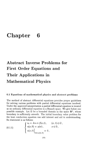
![376 6. Abstract Problems for First Order Equations
where G = f~ x [0, T] is a cylindrical domain. When adopting X
as a basic Banach space, we introduce in the space X a linear (unbounded)
o
operator A = A with the domain T~(A) = W~(f~) O W2’(ft) and call
the Laplace operator. The function u(x,t) is viewed as an abstract
function u(t) of the variable t with values in the space X. Along similar
lines, the function f(z, t) regards as a function with values in the space X,
while the function ~(x) is an element ~ X,making it possible to tre at
the direct problem (6.1.1) ~ the Cauchy problem in the Banach space
for the ordinary differential equation
u’(t) = Au(t) + f(t), 0 <
(6.1.2)
~(0) = p.
Recall that the boundary conditions for the function u involved in (6.1.1)
are included in the domain of the operator A.
The well-founded choice of the basic space X owes a debt to severM
important properties amongw hich the we]]-posednesso f the Cauchyp rob-lem,
a need for differentia] properties of a solution with respect to a spatial
variable and others. Such a setting is mucha ~plicab]e for non-normeda nd
locally convex topologicM vector spaces which are used in place of the Ba-nach
space just considered. Also, in some cases the space X is replaced
by a scale of Banach spaces. Within a wide range of applications which
do ~rise in the sequel, the space X is ~resupposedto be B~nachu nless
otherwise is explicitly stated.
mhem ~in id~ behind ~ ~tur~l ~pp~o~cht o p~obl~m~(~ .l.1)-(~.l.2)
is that all of the basic relations should occur in a pointwise sense. However,
there-is somed ifference betweenp roblems( 6.1.1) and (6.1.2). The essense
of the ma~teris that the operationo f differentiation with respectt o ~ is per-formed
in a dissimilar sense for both cases. In particular; the t-derivative
~rising in problem( 6.1.2) is to be understooda s a limit of the correspond-ing
difference relagion in the normo f the space X. Whens olutions of both
problemsa re treated as distributions, the dissimilarity betweenth emw ill
disappear. A generalized solution of problem (6.1.2) can uniquely be as-sociated
with a distribution from the class ~’(G) subject to (6.1.1)
certain sense. Becauseo f this, the exploration of problem( 6.1.2) is some-what
different from that of problem( 6.1.1) by meanso f special methods,
~hose use permits us to reveal some properties peculiar to the regularity
of generalizeds olutions to the heat conductione quationi n the class
~or the purposes of ~he present chapter it would be su~cient to operate
only with continuous solutions of problem (6.1.2). A rigorous definition
such solutions will appear in the next section.
Before proceedingt o a commosne tting, we would like to discuss some
statements of inverse problems and their abstract analogs. Recent years](https://image.slidesharecdn.com/0824719875inverse-141031173353-conversion-gate01/85/0824719875-inverse-397-320.jpg)
![6.1. Abstract problems 377
have seen plenty of publications in this field with concern of the main
mathematical physics equations. We refer the reader to Beals and Pro-topescu
(1987), Birman and Solomyak (1987), Bykhovsky (1957),
and Lions (1972), Fujita and Kato (1964), Guirand (1976), Hejtmanek
(1970, 1984), Henry (1981), Ikawa (1968), Jorgens (1968), Kato (1975a,b),
Kato and Fujita (1962), Lax and Phillips (1960), Lehner and Wing (1955),
Lekkerkerker and Kaper (1986), Massey (1972), Mizohata (1959a,b, 1977),
Montagnini (1979), Phillips (1957, 1959), Richtmyer (1978, 1981), Pdbaric
(1973), Sanchez-Palencia (1980), Shikhov (1967, 1973), Sobolevsky (1961),
Temam(1 979), Vidav (1968, 1970), Voight (1984) and Yakubov( 1985).
pecial attention in the subsequent studies is being paid to some properties
peculiar for some operators by means of which the subsidiary information is
provided. There exist two typical situations, where in the first the function
f as a membero f equation (6.1.1) is of the structure
(6.1.3) f(x,t) = 02(x,t) p(t),
where the function q~ is known in advance and the unknown function p
is sought. In trying to recover the function p we have to absorb some
additional information. One way of proceeding is to describe the solution
behavior at a fixed point of the domain f~ by the relation
(6.1.4) U(xo,t) = ¢(t), 0 < t < T,
where ¢ is some known function defined on the segment [0, T]. Other
ideas with abstract forms are connected with the following setting. When
working in the space Y = R, we assume that the functions ¢ and p fall into
the category of abstract functions of the variable t with values in the space
Y. The symbol qS(t) designates, as usual, the operator of multiplication
of an element p E Y by the function ¢2(x,t) being viewed as a function of
the variable x with a fixed value t. If the function q5 is sufficiently smooth
(for example, under the premise that for any fixed argument t E [0, T] the
function (I)(x, t) as a function of the variable x belongs to the space L2(f~)),
then O(t) acts from the space Y into the space X. When this is the case,
we may attempt relation (6.1.3) in the abstract form
(6.1.5) f(t) = ~(t)p(t),
where the operator ~(t) E £(Y, X) for any t E [0,
In the space X = L2(~) the operator B acting in accordance with the
rule
B u = u(x0)](https://image.slidesharecdn.com/0824719875inverse-141031173353-conversion-gate01/85/0824719875-inverse-398-320.jpg)
![378 6. Abstract Problems for First Order Equations
is defined on the set of all continuous in ft functions and is aimed to derive
an abstract form of relation (6.1.4). On that space the operator B becomes
a linear functional from X into Y, so that relation (6.1.4) can be rewritten
as
(6.1.6) B ~(~) = ¢(0, 0 < t < T.
Whene quation (6.1.2) is adopted as a relation satisfied in a pointwise
sense, we take for granted that for any fixed value t e [0, T] the element u(t)
o
belongs to the space 7)(A) = W~(ft) ~1 W~(ft). Embedding theorems
Sobolev’s spaces yield W~(f~) C C(~)) for any bounded three-dimensionM
domain ft and, therefore, the operator B is defined on any solution to
equation (6.1.2). However, this operator fails to be bounded and even
closed. On the other hand, if the manifold 7)(A) is equipped with
graph norm, that is, with the W~(ft)-norm, then the operator B acting
from 7)(A) into Y becomes bounded:
(6.1.7) B ¯ £(T~(A),
Additional information may be prescribed in an integral form as well.
The following example helps motivate what is done. The subsidiary infor-mation
here is that
(6.1.8)
Rela~;ion (6.1.8) admits an interesting physical interpretation as a result
of measuring the temperature u by a perfect sensor of finite size and, in
view of this, performs a certain averaging over the domain fL Observe that
(6.1.8) takes now the form (6.1.6) with the operator B incorporated:
B u = f u(x) w(~)
Holding w ¯ L2(ft) fixed we will show that
(6.1.9) B ¯ £(X, Y).
Indeed, when (6.1.8) is the outcome of measuring the temperature by
real sensor, there is a good reason to accept th.at the function w is smooth
and finite in the domain ft. In the case of a sufficiently smooth boundary
of the domain ft the Laplace operator is self-adjoint and
0 V(A*)= w:(ft)](https://image.slidesharecdn.com/0824719875inverse-141031173353-conversion-gate01/85/0824719875-inverse-399-320.jpg)
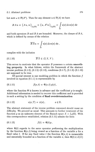
![3so 6. Abstract Problems for First Order Equations
for any fixed value t ¯ [0, T]. What is more, condition (6.1.12) can
rewritten as
(6.1.14) u(T) =
where ¢ is a known element of the space X.
It is necessary to indicate a certain closeness between the statements of
the inverse problems (6.1.1), (6.1.3)-(6.1.4) and (6.1.1), (6.1.11)-(6.1.12).
In the first one the unknownc oefficient of the source term depends solely on
t and in this case the subsidiary information is also provided by a function
depending on t. In the second one the same principle is acceptable for
action: the unknown part of the source and the function built into the
overdetermination condition depend only on one and the same variable x.
Such a closeness emerged in the abstract analogs of the inverse problems
posed above. This is especially true for (6.1.2), (6.1.5)-(6.1.6) and (6.1.2),
(6.1.13)-(6.1.14). In the first setting being concerned with a function
the variable t with values in the space Y we are trying to find a function
of the variable t with value~ in the space Y. In another abstract inverse
problem an element p E X is unknown and the subsidiary information is
that ¢ is an element of the same space X.
There are no grounds to conclude that the principle formulated above
is not sufficiently universal to cover on the same footing all possible state-ments
of inverse problems arising in theory and practice. In dealing with
problems of another nature (being not inverse) one can encounter other
statements in which the unknown parameter and the subsidiary informa-tion
are connected with functions of several variables. Such settings find a
wide range of applications, but do not fit our purposes within the uniform
abstract framework and need special investigations. Just for this reason
we focus our attention here on such statements of inverse problems, whose
constructions not only provide one with insight into what is going on in
general from a uniform viewpoint, but also permit one to get quite complete
answers to several principal questions of the theory.
6.2 The linear inverse problem
with smoothing overdetermination:
the basic elements of the theory
Let X and Y be Banach spaces. We have at our disposal a closed linear ¯
operator A in the space X, whose domain is dense. Under the natural
premises ~ ¯ C([0, T]; £( Y, X )), F C([0, T] ; X ), B ¯ £(X,Y )
¢ ¯ C([0, T]; Y), u0 ¯ X we consider the inverse problein of finding](https://image.slidesharecdn.com/0824719875inverse-141031173353-conversion-gate01/85/0824719875-inverse-401-320.jpg)
![6.2. Basic elements of the theory 381
a pair of the functions ~ ~ C([0, T]; X) and p ~ C([0, T]; V) from the
of relations
(6.2.1) u’(t) = Au(t)+f( t), 0<t <T,
(6.2.2) ,,(0) = ~o,
(6.2.3) f(t) = ~(t)p(t) + 0 < t < T,
(6.2.4) Bu(t) : ~b(t), 0 < t < T.
Since only continuous solutions are considered, equation (6.2.1) is to
understood in a sense of distributions. Recall that the the operator A is
closed. Consequently, the domain of A becomes a Banach space in the
graph norm, making it possible to deal with distributions taking the values
from the manifold 79(A). The meaning of relation (6.2.1) is
~ e v’((o, T), v(A))
and for any function ~ ~ 79(0, T) we should have
Because the function u is continuous from the segment [0, T] into the space
X, the remaining relations (6.2.2)-(6.2.4) are meaningful.
At first glance the well-posedness of the Cauchy problem (6.2.1)-
(6.2.2) needs certain clarification. We assume that the operator A gen-erates
a strongly continuous semigroup V(t), that is, the class of operators
in L;(X) which are defined for t >_ 0 and satisfy the following conditions:
(1°) for any x ~ X the function V(t)x is continuous for all t >_ 0 in the
space X;
(2 0) V(O)=~;
(30) V(t+s)=V(t)V(s) for anyt, s>_O.
The operator A is just a strong derivative at zero of the semigroup it
generates and, in so doing,
fz~X: 31im V(t)- V(O) ~
t--*O ~ J ’
A x = lim V(~)-V(O..)](https://image.slidesharecdn.com/0824719875inverse-141031173353-conversion-gate01/85/0824719875-inverse-402-320.jpg)
![382 6. Abstract Problems for First Order Equations
For the operator A to generate a strongly continuous semigroup the Hille-
Yosida condition is necessary and sufficient, saying that there is a whole
ray A > A0 contained in the resolvent set of the operator A and there is a
constant M :> 0 such that on that ray its resolvent R(A, A) obeys for any
positive integer n the estimate
(6.2.5) M
II R(AA,) ’
This condition holds true if and only if the Cauchy problem (6.2.1)-(6.2.2)
is uniformly well-posed in the class of strong solutions
u e C~ ([0, T]; X) ~ C([O, T]; V(A))
The Hille-Yosida condition is also sufficient for this problem to be well-posed
in the class of distributions. For more a detailed exposition of the
well-posedness of the Cauchy problem and the relevant properties of op-erator
semigroups we recommend to see Balakrishnan (1976), ClEment
al. (1987), Dunford and Schwartz (1971a,b,c), Fattorini (1983), Goldstein
(1985), Henry (1981), Hille and Phillips (1957), Kato (1966), Krein
Mizohata (1977), Pazy (1983), Trenogin (1980), Yosida (1965). It
be noted here that under the conditions imposed above the Cauchy prob-lem
(6.2.1)-(6.2.2) has a continuous solution u e C([0, T]; X) for
function f e C([0, T]; X ) and any element u0 e X, this solution is unique
in the indicated class of functions and is given by the formula
u(t) : V(~) Uo + / V(~- s) f(s)
0
If, in addition, f e Cl([0, TI;X) -[-C([0, TI;7)(A)) and u0 e 79(A),
formula (6.2.6) specifies a strong solution
¯ T];X) C([O,
The assumptions to follow are concerned with some properties of the
operator B, which is in charge of surplus information in the form of overde-termination.
This operator is supposed to possess £ smoothing effect,
meaning
(6.2.7) B, BA e £,(X, Y).
Theorem 6.2.1 Let the closed linear operator A with a dense domain
generate a strongly continuous semigroup in the space X, condition (6.2.7)](https://image.slidesharecdn.com/0824719875inverse-141031173353-conversion-gate01/85/0824719875-inverse-403-320.jpg)
![6.2. Basic elements of the theory 383
hold and¯ E C([0, T];£(Y,X))F, ~ C([0, T];X), Uo~ X and~ ~
C~([0T, ];r ). Zffora ny~ ~ [0, T]t heo perat~oOr (ti)s in~ertib~e,
(B~) -~ ~ c([o, T];
and the compatibility condition B uo = ¢(0) holds, then a solution u,
of the inverse problem (6.2.1)-(6.2.4) exists and is unique in the class of
functions
~ Ec ([o, T]; x), p ~ C([OT, ];
Proof Formula (6.2.6) implies that a solution of the Cauchy problem
(6.2.1)-(6.2,2) can be expressed
t t
0 0
Therefore, condition (6.2.4) is equivalent to the following equation:
(6.2.8)
t
B( v( luo+f v(t-sl (s p(sl
0
t
¢(t), o < t < T.
The equation thus obtained contains only one unknown function p and the
question of existence and uniqueness of a solution of the inverse problem
(6.2.1)-(6.2.4) amounts to the question of existence and uniqueness
continuous solution to equation (6.2.8). At the next stage we are going
to show that equation (6.2.8) can be differentiated. The following lemmas
will justify the correctness of this operation.
Lemma 6.2.1 For any Uo ~ X the function g(t) = B V(T) Uo is continu-ously
differentiable on the segment [0, T] and
d(t) = B A V(t)
Proof Holding A ~ p(A) fixed and setting
ul = (A - AI)-1 Uo,](https://image.slidesharecdn.com/0824719875inverse-141031173353-conversion-gate01/85/0824719875-inverse-404-320.jpg)
![384 6. Abstract Problems for First Order Equations
we thus have ul E :D(A) and
(V(t) ul)’ = V(t) AUl = AY(t)
Furthermore, it is straightforward to verify that
g(t) = BV(t)(A-AI)Ul = BAV(t)ul-ABV(t)ul
and, since both operators B A and B are bounded, find that
g’(t) = BA(V(t)u~)’-AB(V(t)u~)’
= BAV(t) Au~-ABV(t)Aul
=BA V(t)(A-~I)ul
= BA V(t) uo.
Lemma 6.2.2 On the segment [0, T] the function
t
g(t) : B / Y(t- s)f(s) ds
0
is continuously differentiable for any continuous in X function f and
g’(t) = B---~ / V(t - s) f(s) ds + B f(t).
0
Proof By analogy with the above lemma the proof is simple to follow.
Holding k E p(A) fixed and setting, by definition,
h(t) = ( A AI)-1 f( t) ,
we deduce that
Ah(t) = ((A- hi)+ hi) (A-.~I) -1 f(t)
:-fI(ft()t)÷,(A-AI)](https://image.slidesharecdn.com/0824719875inverse-141031173353-conversion-gate01/85/0824719875-inverse-405-320.jpg)
![6.2. B~sic elements of the theory
so that
(6.2.9) h, Ahe C([0, T]; X).
On the other hand,
g(t) = B / V(t - s) ( A - ~ I ) h(s)
0
t
= (B A - ~ B) J V(t - ~)
0
From condition (6.2.9) it follows that
t
v(t - ~) h(~) = u(t - ~) A h(~) d~ +
0 0
and, due to the boundedness of both operators B A and B,
0
Since B A C B A, we find that
0
~rom the definition of ghe Nnc~ion h it seems clear that
or, what amounts to the same,
~h(~) = ah(~ + ~(t).
With the relation h(~) ~ ~(A), ~ e [0, T], in view, we deduce
~ ~ h(~l = ~
385](https://image.slidesharecdn.com/0824719875inverse-141031173353-conversion-gate01/85/0824719875-inverse-406-320.jpg)
![6.2. Basic elements of the theory 387
From the conditions of the theorem and relations (6.2.11)-(6.2.12) we
duce that the function P0 is continuous on the segment [0, T] and the
operator kernel K(t, s) is strongly continuous for 0 < s < t < T. These
properties are sufficient for the existence and uniqueness of the solution to
the integral equation (6.2.10) in the class of continuous functions in light
of results of Section 5.1 and thereby the theorem is completely proved. ¯
Having established the unique solvability of the inverse problem
(6.2.1)-(6.2.4) we should decide for ourselves whether the solution in ques-tion
is continuously dependent on the available input data.
Theorem 6.2.2 Under the conditions of Theorem 6.2.1 there exists a pos-itive
constant M = M(A,B,¢,T) such that a solution u, p of the inverse
problem (6.2.1)-(6.2.4)satisfies lhe eslimates
II ~I Ic(I0,rl;x-<) M @ U oI Ix +I I ¢ Ic,(t0T l;r)+ II v I c(~0,w~.x)),
IIP~I~(~0,T63 M;~( 131 ~ ollj+ II¢ Ile,(~0,~v;) IIFlclC~o,~;x3 ).
Proof To derive the second inequality one can involve the integral equation
(6.2.10), whose solution does obey the estimate
IlPllc(lo,~3;MY1I)l po
where the constant M~ depends only on the kernel of this equation, that
is, on A, B, ¯ and T. On the other hand, relation (6.2.11) implies that
II p0I Ic<iO,yT)~ ~M ; (~1 1U oII x+ IIW II C’(~0y,T)+ ~I ;I f IIc<~T0~, ;
which justifies the desired estimate for the %nction p. Here the constant
M2 depends only on A, B, ~ and T. With regard to the function u formula
(6.2.6) applies equally well to the decomposition
yielding
where the constant Ma depends only on A and T. Since
II f Ile([0,r]; x) 5 M4( ll P IIc([0, T]; + II F lice[0, r];X) )
with constant M4 depending solely on ¯ and T, the desired estimate for
the function p is a simple implication of the preceding inequalities and the
estimate for the function u we have established at the initial stage of our
s~udy. This compleges the proof of the theorem.~](https://image.slidesharecdn.com/0824719875inverse-141031173353-conversion-gate01/85/0824719875-inverse-408-320.jpg)
![388 6. Abstract Problems for First Order Equations
It is interesting to know when equation (6.2.1) is satisfied in a point-wise
manner. In this regard, there arises the problem of finding out when
the solution of the inverse problem concerned,satisfies the condition
u e c1([0,T ];x ) Nc ([0,T ];P (A)).
Because the function f involved in the right-hand side of equation (6.2.1)
continuous, the belonging of u to the space C([0, T]; ~(A)) will be proved
if we succeed in showing that u ¯ C1 ([0, T]; X). One well-known fact
from semigroup theory may be of help in achieving the final aim: if the
function f ¯ C1 ([0, T]; X) and the element u0 ¯ D(A), then the function
u specified by formula (6.2.6) is continuously differentiable on the segment
[0, T] in the norm of the space X, so that
(6.2.1a)
t
u’(t) : V(t) (Auo f( 0)) + V(t - s) f’ (s) ds.
o
If f admits the form
with the members
f(t) + F(t)
¯ ¯ C1 ([0, T]i £(Y, X)), r ¯ c1 ([o, x),
then the continuous differentiability of the function p would be sufficient for
the function f to be continuously differentiable. Just for this reason a pos-itive
answer to the preceding question amounts to proving the continuous
differentiability of a solution to the integral equation (6.2.10).
Theorem 6.2.3 Let the closed linear operator A with a dense domain be
the generator of a slrongly continuous semigroup in the space X, condition
(6.2.7) hold, ¯ ¯ el(J0, T]; £:(Y,X)), ¯ Cl ([0, T] ; X), ?. o ¯ ~ (g),
~b ¯ C2([0, T]; Y), for any t ¯ [0, T] the operator l3C~(t) be invertible and
(B q~) -~ e C~ ([0, T]; £(Y)). If the compatibility condition B Uo = ¢(0) is
fulfilled, then a solution of the inverse problem (6.2.1)-(6.2.4) exists and is
unique in the class of functions
~t ¯ cl ([0, T]; X) N C([0, r]; D(A)), p ¯ C1 ([0, ~E’]j y)
Proof As stated above, it is sufficient to prove that under the premises
of the theorem a solution to the integral equation (6.2.10) is continuously
differentiable. This can be done using equation (6.2.10) together with the](https://image.slidesharecdn.com/0824719875inverse-141031173353-conversion-gate01/85/0824719875-inverse-409-320.jpg)
![39o 6. Abstract Problems for First Order Equations
Let us consider the system of integral equations
t
p(t) = po(t) + / If(t, s)p(s)
0
t t
q(t) = qo(t)+ / Kl(t,s)p(s) ds+ / K(t,s)
which has a unique continuous solution. This is due to the continuity of the
functions P0 and q0 and the strong continuity of the operator kernels K(t, s)
and Kl(t, s) (for more detail see Section 5.1). Moreover, this solution can
be obtained by means of the successive approximations
t
(6.2.18)
0
t
(6.2.19) 4,~+1(t) qo(t)+ j K~(t, s) ~(s) ds
0
+ / s) ds,
0
which converge as n --~ c~ to the functions p and q, respectively, uniformly
over the segment [0, T]. In light of the initial approximations/50 = 0 and
40 = 0 it is reasonable to accept
Assuming that there exists a positive integer n, for which the equality
= p. is true, we will show by differentiating (6.2.18) that this equality
continues to hold for the next subscript. In giving it all the tricks and tucks
remain unchanged as in the derivation of equation (6.2.14). The outcome
of this is
t t
~+~(t) = qo(t) + / K~(t,s)~(s) K(t,s)~(s) ds.
Comparison with (6.2.19) shows that ~.+~ = p~+~. We deduce by induction
on n that the equality](https://image.slidesharecdn.com/0824719875inverse-141031173353-conversion-gate01/85/0824719875-inverse-411-320.jpg)
![6.2. Basic elements of the theory 391
is valid for any positive integer n.
Therefore, the sequence/Sn converges as n --~ ~ to the function p
uniformly over the segment [0, T]. At the same time, the sequence /5~
converges uniformly to the function q. From such reasoning it seems clear
that p is continuously differentiable and p~ = q, thereby completing the
proof of the theorem.[]
The next step of our study is connected with various estimates for
the derivatives of the inverse problem solution similar to those obtained
in Theorem 6.2.2 and the existing dependence between its smoothness and
the smoothness of the input data. The questions at issue can be resolved
on the same footing if the derivatives of the inverse problem (6.2.1)-(6.2.4)
solution (if any) will be viewed as the continuous solutions of the same
problem but with other input data known as the "problem in varia-tions".
This approach is much applicable in solving nonlinear problems,
since the emerging "problem in variations" appears to be linear. However,
this approach provides proper guidelines for deeper study of many things
relating to linear problems as well.
Theorem 6.2.4 Lel the conditions of Theorem 6.2.3 hold, a pair of lhe
functions u, p solve the inverse problem (6.2.1)-(6.2.4),
Wo = A uo + f(O) G = ¢’ p + F’
and ~ = ¢’. Then the functions w = u’ and q = p’ give a continuous
solution of the inverse problem
(6.2.20) w’(t) = A w(t) g(t)., 0 < t < T,
(6.2.21) w(O) = Wo,
(6.2.22) g(t) = if(t) q(t) + 0 < t < T,
(6.2.23) B w(t) = ¢,v(t), 0 < t < T.
Proof Since the function p is continuously differentiable, the function
f = i p+ F G C1([0, T]; X).
Because of this fact, we might rely on formula (6.2.13) as further develop-ments
occur. Substituting g = fl and retaining the notations of Theorem
6.2.4, we recast (6.2.13)
t
o(t) = v(t) + / v(t - s) g(s)ds.
0](https://image.slidesharecdn.com/0824719875inverse-141031173353-conversion-gate01/85/0824719875-inverse-412-320.jpg)
![6.2. Basic elements of ~he ~heory 393
thereby justifying the first and third estimates of Corollary 6.2.1. As can
readily be observed, the relation
A u(t) : u’(t) - (I)(t) p(t) - F(t)
holds true on the strength of (6.2.1) and (6.2.3), so that the second inequal-ity
arising from Corollary 6.2.24 becomes evident by successively applying
the preceding estimates for u’ and p to the right-hand side of (6.2.24). This
proves the assertion of the corollary. ¯
The result obtained in Theorem 6.2.4 may be of help in revealing
the dependence between the smoothness of the inverse problem solution
and the smoothness of the input data. Being a solution of the inverse
problem (6.2.20)-(6.2.23), the functions w and q give the derivatives of
corresponding solution of the inverse problem (6.2.1)-(6.2.4). With this
mind, the conditions of continuous differentiability of the inverse problem
(6.2.20)-(6.2.23) solution turn into the conditions of double continuous
differentiability of the inverse problem (6.2.1)-(6.2.4) solution.
In trying to obtain these conditions we make use of Theorem 6.2.3
with regard to the inverse problem (6.2.20)-(6.2.23). Careful analysis
its premises shows that it would be sufficient to achieve ~ ¯ C2 ([0, T];
£(Y,X)), F C~([O, T] ; X), Au o + f( O) ¯ D(¢ ¯ Ca (J 0, T]; Y),
B u0 = ¢(0) and
B (duo + f(0)) --= ¢’(0).
This type of situation is covered by the following assertion.
Corollary 6.2.2 Let the closed linear operator A with a dense domain be
the generator of a strongly continuous semigroup in the space X, condition
(6.2.7) hold and (b ¯ C2([0, T]; £(Y,X)), F C2([0, T] ; X), Uo¯ D(A
Auo + f(0) ¯ D(A), ¢ ¯ Ca([0, Y), Buo = ¢( 0) and
B (A u0 + f(0)) = ¢’(0).
If for any t ¯ [0, T] the operator Be(t) is invertible and
(B ,)-~ ¯ 1 ([0, T]; z(Y)),
then a solution u, p of the inverse problem (6.2.1)-(6.2.4) exists and is
unique in the class of functions
u ¯ c~([o,T ];x ), v ¯ c~([o,~ ]; v).](https://image.slidesharecdn.com/0824719875inverse-141031173353-conversion-gate01/85/0824719875-inverse-414-320.jpg)
![394 6. Abstract Problems for First Order Equations
In this context, one thing is worth noting. This is concerned with
the value f(0). Although the function f is supposed to be unknown in the
statement of the inverse problem (6.2.1)-(6.2.4), the value f(0) can
be found from equality (6.2.3), implying that
f(0) = a(0) p(0)
Combination of (6.2.11) and (6.2.12) gives for t = 0 the equality
p(0) = 0(0) (¢,(0) - F(0))
and, because of its form, the compatibility conditions
Au0 + f(0) E ~(A), B (Auo+ f(0))
can be rewritten only in terms of the input data of the inverse problem
(6.2.1)-(6.2.4). The reader is invited to carry out the appropriate manip-ulations
on his/her own.
In concluding this section it remains to note that in Theorem 6.2.3
and Corollary 6.2.2 the differentiability condition for the function ( B ¯ )
can be replaced by the continuity condition for the same function. This is
due to the fact that the differentiability of (Bq~)-1 is an implication of
the well-known formula for the derivative of the inverse operator
[A-l(t)]’ = -.A-~ A’(t) A-~(t).
A final remark is that the procedure of establishing the conditions
under which the inverse problem solution becomes more smooth can be
conducted in just the same way as we did before. Using Theorem 6.2.4
with respect to the inverse problem (6.2.20)-(6.2.23) we might set up
inverse problem for the second derivatives of the problem (6.2.1)-(6.2.4)
solution. The inverse problem thus obtained is covered by Theorem 6.2.3
and so the conditions of triple continuous differentiability of the problem
(6.2.1)-(6.2.4) solution are derived without any difficulties. Going further
with this procedure we reach a solution as smooth as we like.
6.3 Nonlinear inverse problems with
smoothing overdetermination: solvability
In the present section we carry over the results of Section 6.2 to the case
of a semilinear evolution equation. Given Banach spaces X and Y, let
A be a closed linear operator in the space X with a dense domain. One](https://image.slidesharecdn.com/0824719875inverse-141031173353-conversion-gate01/85/0824719875-inverse-415-320.jpg)
![6.3. Problems with smoothing overdetermination: solvability 395
assumes, in addition, that the operator A generates a strongly continuous
semigroup V(t) and the operator B satisfies the following inclusions:
(6.3.1) B, BA
We are interested in recovering a pair of the functions u e C([0, T]; X
and p ~ C([0, T]; Y) from the system of relations
(6.3.2)
(6.3.3)
(6.3.4)
where
u’(t) = Au(t)+ f(t, u(t),p(t)),
u(0) = u0,
B u(t) = ¢(t), 0 < t
f: [O,T]xXxY~X
is a continuous function. Omitting some details related to the concept
of the generalized solution to equation (6.3.2) we mean by a continuous
solution of the Cauchy problem (6.3.2)-(6.3.3) a continuous solution
to the integral equation
t
(6.3.5) ~(t) v(t)~o+/ V(t - s) f( s, u(s),p(s)) ds.
0
Furthermore, we take for granted that the function f has the structure
(6.3.6) f(t,u,p) = fl(t,u) + f2(t,u,p).
The main idea behind decomposition is that the properties of the function
fl should be somewhat different from those of the function f2 due to the
limitations imposed. Representation (6.3.6) is similar to (6.2.3) involved
in the exploration of the linear inverse problem posed completely in the
preceding section. Although the character of (6.3.6) is not quite typical
for a nonlinear problem, it may be of help in investigating some particular
questions at issue.
Let us introduce the following notations:
Sx(a,R)= {~¢~X: Ila-alix<R},
Sx(a,R,T )= {(t,x): O < t < T, X e Sx(a,n)}
Allowing the function ¢ to be differentiable we define the value
(6.3.7) z0 = ¢’(0) BAuo - Bf~(O, uo](https://image.slidesharecdn.com/0824719875inverse-141031173353-conversion-gate01/85/0824719875-inverse-416-320.jpg)
![6. Abstract Problems for First Order Equations
and require then the following:
(A) the equation 13 f2(O, Uo,p) = zo with respect to has a solution
Po E Y and this solution is unique in the space Y;
(B) there exists a mapping
~: [O,T] x Y x Y ~ Y
such that
(C) there exists a number 1~ > 0 such that for any t ~ [0, T] the map-ping
z = ~(t, ¢(t),p) as a function of p is invertible in the
Sy (Po, R) and has the inverse
(6.3.s) p = z);
(D) there is a number R > 0 such that both functions fa(t,u) and
f~(t,u,p) are continuous with respect to the totality of variables
on the manifold Sx×v ((no, Po), R, T) and satisfy thereon the
schitz condition with respect to (u, p);
(E) there is a number R > 0 such that the mapping (6.3.8) is continu-ous
with respect to (t, z) on the manifold Sy(Zo, R, T) and satisfies
thereon the Lipschitz condition in z.
Theorem 6.3.1 One assumes that the closed linear operator A, whose do-main
is dense, generates a strongly continuous semigroup in the space X
and conditions (6.3.1) and (6.3.6) hold. Let u0 E X, ¢ E C1([0, T]; Y)
and 13 Uo = ¢(0). Under conditions (A)-(E), where Zo is defined (6. 3.7),
there exists a value T~ > 0 such that on the segment [0, T1] the inverse prob-lem
has a solution u, p and this solution is unique in the class of functions
u e c([o, TIpx ), p e c([o,T ];Y ).
Proof The conditions of the theorem imply that for any functions
C([0, TIp X ) and p e C([0, TIP Y ) the function
f(t) = f( t, u(t),](https://image.slidesharecdn.com/0824719875inverse-141031173353-conversion-gate01/85/0824719875-inverse-417-320.jpg)
![398 6. Abstract Problems for First Order Equations
At the first stage we are going to show that for a sufficiently small
value T > 0 the system (6.3.9), (6.3.t2) has a unique continuous solution.
On account of the inclusion go E C([0, T]; Y) the function gl(t,u)is con-tinuous
with respect to (t, u) on the manifold Sx (uo, t7, T) and satisfies
thereon the Lipschitz condition in u. The kernel K(t, s) is strongly con-tinuous
for 0 < s < t < T. The second step is to replace (6.3.12 by the
equation
(6.3.13) p(t) =¢(t, go(t) + gi (t, ul(t))
where
t
(6.3.14)
0
The couple of the resulting equations (6.3.9) and (6.3.12) is evidently equiv-alent
to the system (6.3.9), (6.3.13). At the next stage we consider
metric space
Z = C([0, T]; Sx(u0,S~) × S~(p0,S~))
and introduce the operator
a: (u, p) ~ (~,, p,),
where Ul is defined by (6.3.14) and p~ coincides with the right-hand side
(6.3.13).
The theorem will be proved if we succeed in finding a positive number
T > 0 for which the operator G has a unique fixed point in the space Z.
The Lipschitz condition for the functions ¯ and f~ implies the in-equalities
(6.3.16) It g,(t, ",(t))ll L II ,~,(t) - v(t) ,Lo
Let M1 = sup0<t<r II v(t)ll. With this constant in view, representation
(6.3.14) yields
t
6.3.17) Ilu,(t)- V(t)~oll <_ M, J Ilf(s,u(s),p(s))ll ds.
0](https://image.slidesharecdn.com/0824719875inverse-141031173353-conversion-gate01/85/0824719875-inverse-419-320.jpg)
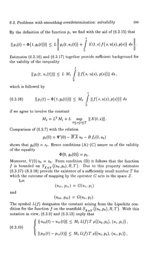
![400 6. Abstract Problems for First Order Equations
where p refers to a metric on the space Z. Estimates (6.3.19) justifies that
there exists a sufficiently small value T, for which G becomes a contrac-tion
operator in the space Z. Thus, the desired assertion is an immediate
implication of the contraction mapping principle, thereby completing the
proof of the theorem. ¯
It is interesting to find out when a solution of the inverse problem
(6.3.2)-(6.3.4) will be differentiable. To provide the validity of this prop-erty,
conditions (D) and (E) necessitate making some refinements. It
be sensible to replace them b~ the following ones:
(Da) there exists a number R > 0 such that both functions fl and
are Frechet differentiable on the manifold Sx ×Y ( ( uo, po), R, T) and
their partial derivatives (fx)t, (fl)~, (f2)~, and (f~)v are con-tinuous
thereon in the operator norm and satisfy the Lipschitz con-dition
with respect to (u,p);
(EI) there exists a number R > 0 such that the function (6.3.8) is Frechet
differentiable on Sv (Zo, R, T) and i~s partial derivatives apt and apz
are continuous in the operator norm and satisfy thereon the Lip-schitz
condition in z.
Theorem 6.3.2 Let the closed linear operator A with a dense domain
generate a strongly continuous semigroup in the space X and conditions
(6.3.1) and (6.3.6) hold, Uo e 73(A), ¢ C2([0, TI P Y)andBuo --: ¢(0)
Under conditions (A)-(C), (Da) and (E~), where Zo is defined (6. 3.7),
there exists a value TI > 0 such that on the segment [0, T1] a solution u, p
of the inverse problem (6.3.2)-(6.3.4) exists and is unique in the class of
functions
u e el(J0, Ta]; X) [~ C([0, Ta]; D(A)), p ¯ c’([0, T,]; r).
Proof First of all observe that conditions (Da) and (Ea) imply conditions
(D) and (E). Hence by Theorem 6.3.1 the inverse problem (6.3.2)-(6.3.3)
has a unique continuous solution for all sufficiently small values T. Since the
function f(t, u(t), p(t)) is continuous, the continuity of the function A u(t)
is ensured by relation (6.3.2) because of the continuity of u’(t). There-fore,
in order to establish the desired assertion, it suffices to justify the
differentiability of the functions u and p both.
l~ecall that these functions give a continuous solution to the system of
the integral equations (6.3.9), (6.3.12), which are currently to be differenti-
Iated and supplemented by the relevant equations for the functions w -- u
and q = pl. By the initial assumptions and relation (6.3.6) there exists](https://image.slidesharecdn.com/0824719875inverse-141031173353-conversion-gate01/85/0824719875-inverse-421-320.jpg)
![6.3. Problems with smoothing overdetermination: solvability 401
value R > 0 such that on the manifold Sxx~. ((u0,p0),/~, T) the function
f(t, u,p) is Frechet differentiable and its partial derivatives f~, f~ and
are continuous and satisfy thereon ~he Lipschitz condition wi~h respec¢ ¢o
(u, p) in ~he operator norm. Moreover, the function
go(*) : ~’(~)- BA V(*)Uo- B ~(~,
will be continuously differentiable in Z on the sp~ce Y ~nd the function
g~(t,u) = -B (f~(t,u)- f~(t, V(t)uo))
will be Frechet differentiable on the manifold Sx (Uo, R, T) and its partiM
derivatives g~,t ~nd g~,~ will be continuous thereon and sutisfy the Lip-schitz
condition with respect to u in the operator norm. Being formally
differentluted equations (6.3.9) and (6.3.12) lead to the chains of relations
(6.3.20) w(t) = V(t)(Auo+ f(O, uo,Po))
t
+ / V(t - s) [ ft (s, u(s),
0
+~ . (~, ~(~)~, (~))
+ fp(s,u(s),p(s)) q(s)] ds,
(6.~.~) ~(t) = ~,(t,~o(t)+ ~(t,~(t))
t
+S K(t,s)f(s,u(s),p(s))
0
0
" (~(+~ a), ,~(,. (0+) a ,.(.~(,0~ )( ~)
+~ ’(o~)f, ( o.,o ,](https://image.slidesharecdn.com/0824719875inverse-141031173353-conversion-gate01/85/0824719875-inverse-422-320.jpg)
![402 6. Abstract Problems for First Order Equations
t
0
+ fu(s, u(sl,P(sl) w(s)
+f p(s~, (s),p (~)q) (~)]
When the functions u E C([0, T]; X ) and p e C([0, T]; Y) are kept fixed,
the system (6.3.20)-(6.3.21) becomes a linear system of the Volterra second
order integral equations related to the functions w and q. The nonhomoge-neous
members of this system are continuous and the kernels are strongly
continuous. Whence it follows that there exists a unique continuous so-lution
to the preceding system and it remains to establish the relations
w = u’ and q = p’. With this aim, we agree to consider
wo = Auo + f(0,Uo,po),
qo = Ct(O, go(O)) + ~z(O, go(O))
× (g~(O) + gl,t(O, ZtO) g,,,,(O, uo ) Wo
+s ,:(oo, )f (o,~ op, c)).
We note in passing that equations (6.3.12) and (6.3.21) are equivalent
the following ones:
(6.3.~2v)( t)
t
0
(6.3.23)
q(t)
t
0
+ ~ (t, ~o(t) + ~(t, ~(t))](https://image.slidesharecdn.com/0824719875inverse-141031173353-conversion-gate01/85/0824719875-inverse-423-320.jpg)
![6.3, Problems with smoothing overdetermination: solvability 403
t
0
x (g~o(t) +gl,t(t, ~(t)) +g~,~(t,. ~(t))ff~(t)
+~ r~(to,) 1 (o~, o,
t
+ f iqt, s) [ s, (s, u(s), p(s))
0
+ f~ ( s, u(s), p(,))
+ fp ( s, u(s), p(s)) q(s)] ds),
where ~(t) are @(t) refer to the right-hand sides of relations (6.3.9)
(6.3.20), respectively.
Let
Z1 = C([O, T]; Sx(uo,R ) x Sy(po,R) x Sx(wo,R ) × Sy(qo,R)).
We deal in that metric space with the operator
where ~ and ~ stand for the right-hand sides of (6.3.22) and (6.3.23),
spectively. The operator G1 so constructed is of the same structure as the
operator G arising from the proof of Theorem 6.3.1. Following the scheme
of proving the preceding theorem we are now in a position to find a suffi-ciently
small value T > 0 for which the operator G1 becomes contractive
on the space Z~. In this view, it is reasonable to employ the method of
successive approximations by means of which a solution of the system of
equations (6.3.9), (6.3.20), (6.3.22) and (6.3.23) can be obtained.
result of such manipulations is as follows:
(6.3.24)
t
~tn+~(t) = V(t)uo + / V(t- s) f( s, ~tn(s),~n(s))
0
Also, the sequences
(6.3.25) t~n+~ (t) V(t) ( A Uo+ S(O, uo, po))](https://image.slidesharecdn.com/0824719875inverse-141031173353-conversion-gate01/85/0824719875-inverse-424-320.jpg)
![404
(6.3.26)
(6.3.27)
6. Abstract Problems for First Order Equations
+ / v(t - ~)[ f~(~r, i~(s),~(~))
o
+ f~(~,r i~(sl,~(s)~) (~)
+ fp(S, rin(s),~n(s)) ~n(s)] ds,
~+~(t) = ¯ ( t, go(t) + g~ 5~+~(t))
t
o
O.+l(t) = ¢, ( t, go(t) + g, ~n+l( t))
o
+* . (~,~ o(~+1~ , (t,
t
o
x (g’o(t)
+ gl,~ (t, ~n+l(t))
0
+ ~ (~, ~(~,~(~)
will be uniformly convergent on the segment [0, T]. The initial approxima-tions
rio(t), ~o(t), 150(t) and ~0(t) may be taken to be zero. Via represen-tations
(6.3.24) and (6.3.26) it is not difficult to deduce by induction
that the functions ri~ and/~ are continuously differentiable for all n.
With the initial assumptions in view, careful analysis of (6.3.4) leads
to
f(t) = f(t,~.(t),#n(t)) CI([O,T];X),](https://image.slidesharecdn.com/0824719875inverse-141031173353-conversion-gate01/85/0824719875-inverse-425-320.jpg)
![6.3. Problems with smoothing overdetermination: solvability 405
so that the function fin+l satisfies the equation
(6.3.28) ~+l(t) - AG~+I(t) = f(t,G~(t),~(t)).
The value A ~n+l can be found from (6.3.24) by the well-known formula
from the theory of semigroups (see Fattorini (1983), Kato (1966)).
t t
A / V(t - s) f(s) ds -- / V(t - s)S’(s) V(t) f(O) f(t)
0 0
which is valid for any continuously differentiable function f. If ~(0) --
and/~,~(0) = P0, then
(6.3.29) A~tn+~(t) =V(t)(Auo+ f(O, uo,Po))
t
+ / v(t - s) [ft(s,~n(s),~n(s))
+ f~ (s, ~,(s),~n(s))
+ f.(~, ~.(~),~.(~~))’ ~(~)]
- f(t, ~n(t),~(t)).
Subtracting (6.3.29) from (6.3.25) yields the relation
t
(v,~+~(t) - A (tn+~(t) = / V(t - s) [ f~ ( s, G~(s),
0
(6.3.30) x (~,~(s) - fi~(s)) f. (s, ~n (s),~n(s))
× (~(s)~ ’~(s)] ~+ f(t, ~(t),~(t)),
from which (6.3.28) can be subtracted. All this enables us to establish the
relationship
(6.3.31)
~+~(t-) ~’~+~(t)
t
0
x (~(~)- ~’~(~)+) ~,(~, ~(s),~(~))
x q.(~)-p.(s](https://image.slidesharecdn.com/0824719875inverse-141031173353-conversion-gate01/85/0824719875-inverse-426-320.jpg)
![406 6. Abstract Problems for First Order Equations
Having (6.3.26) differentiated we subtract the resulting expression from
(6.3.27) and, after this, arrive
~n+l(t) ¯ ~ (t,go(t) gl(t, ~n+l(t))
t
o
× (gl,u(t,~n+l(t)) (~n+l(t) -- fi~n+l(t))
t
0
With zero initial approximations, the equalities
and
become valid. With the aid of relations (6.3.31)-(6.3.32) we derive
induction on n the equalities ~,~= fin and ~ = ~P1n, valid for all n E N, and
involve these as further developments occur. Therefore, the sequences fi,~ --~
u, u,~ -~ w, i5~ --~ p andp,~ ~’ --* q as n --* o~ uniformly over the segment
[0, T]. Finally, the functions u and p are continuously differentiable, thus
causing the needed relations u~ = w and pl = q and completing the proof
of the theorem.m
6.4 Inverse problems with smoothing overdetermination:
smoothness of solution
We begin by considering the inverse problem (6.3.2)-(6.3.4) in another
sion giving a generalization of setting up problem (6.2.1)-(6.2.4) under](https://image.slidesharecdn.com/0824719875inverse-141031173353-conversion-gate01/85/0824719875-inverse-427-320.jpg)
![6.4. Problems with smoothing overdetermination 407
agreement that the function f involved in equation (6.3.2) is representable
by
(6.4.1) f(t,u,p) ~= Ll(t)u + L~(t)p+ F(t),
where L~(t) ¯ £(X), L~(t) ¯ £(Y, andF(t) ¯ X f orevery fixed t ¯
[0, T]. In that case the unique solvability is revealed on the whole segment
[0, T] as occurred in the inverse problem (6.2.1)-(6.2.4). For the reader’s
convenience the complete statement of the inverse problem amounts to
finding a pair of the functions u ¯ C([0, T]; X ) and p ¯ C([0, T]; Y )
the system of relations
(6.4.2)
(6.4.3)
(6.4.4)
u’(t) = A u(t) + L1 (t)
+ L (t) p(t) + F(t),
u(O)
B u(t) = ¢(t), 0 < t
0<t<T,
where the operator B is in line, as before, with the inclusions
(6.4.5) B,BA ¯ £(X,Y)
and equation (6.4.2) is to be understood in a sense of distributions.
Theorem 6.4.1 One assumes that the closed linear operator A, whose
domain is dense, generates a strongly continuous semigroup in the space X
and condition (6.4.5) holds. Let
La ¯ C([0, T]; £(X)) L2 ¯ £([0, T]; £(Y, X)),
F ¯ C([0, T]; X), Uo ¯ X, ¢ ¯ C1 ([0, T];
When t ¯ [0, T] is kept fixed, the operator B L2 (t) is supposed to be invert-ible
and
(B L~)-~ ¯ C([0,
ff the compatibility condition B Uo = ¢(0) is fulfilled, then a solution u, p
of the inverse problem (6.4.2)-(6.4.4) exists and is unique in the class of
functions
u ¯ C([0, T]; X), p ¯ C([0, T];](https://image.slidesharecdn.com/0824719875inverse-141031173353-conversion-gate01/85/0824719875-inverse-428-320.jpg)
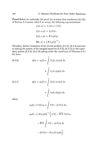
![6.4. Problems with smoothing overdetermination 409
K~(t,s) = V(t - s) Ll(s),
L~(t,s) = V(t - s) L~(s),
K~(t,s)= - ( BL ~(t)-)1 ( BA V (t -
× L,(s) + B L, (t) K~(t,
L~(t,s)= - ( Bm 2(t)-)1 ( BA V (t -
x L~(s) +BL~(t)L~(t,s)).
It is worth bearing in mind that the premises of this theorem imply the
strong continuity of the operator kernels K~, L~, K~, L~ for 0 < s < t <
T as well as the continuity of the functions no(t) and po(t). We know
from Section 5.1 that these properties are sufficient for the system of the
Volterra integral equations (6.4.6)-(6.4.7) to have a unique solution
in the class of continuous functions, thereby completing the proof of the
theorem.I
If the input data functions possess the extra smoothness, then the
same property would be valid for a solution. The analog of Theorem 6.3.2
in the linear case of interest is quoted in the following proposition.
Theorem 6.4.2 One assumes that the closed linear operator A, whose
domain is dense, generates a strongly continuous semigroup in the space X
and condition (6.4.5) is satisfied. Let
L1 e C1([0, T]; ~(X)) , L2 1( [0, T]; ~(Y~ X)),
~ e c1 ([o, T]; x), u0 ¯ ~(A)
and ¢ ¯ C2([0, T]; Y ). If, for any fixed value t ¯ [0, T], the operator
B L~(t) is invertible,
( B L~)-i ¯ C1([0, T]; £(Y))
and the compatibility condition B uo = ¢(0) holds, then a solution u, p
of the inverse problem (6.4.2)-(6.4.4) exists and is unique in the class of
functions
/Z ¯ CI([0, T]; X) f~ C([0, T]; V(A)) /9 ¯ cl([o, T];](https://image.slidesharecdn.com/0824719875inverse-141031173353-conversion-gate01/85/0824719875-inverse-430-320.jpg)
![410 6. Abstract Problems for First Order Equations
Proof First of all note that the conditions of the theorem provide the
validity of conditions (D1) and (El) as well as reason enough for differenti-ating
the system (6.4.6)-(6.4.7) and extending it by joining with equations
(6.3.20) and (6.3.23). The system thus obtained is linear and can be written
(6.4.8) u(t) = uo(t)
t
[ul(t,s)~(s+) u~(t,s)p(s)]
(6.4.9) p(t) = po(t)
t
[P~(t, s) u(s) + P~(t, s)p(s)]
(6.4.10) w(t) = Wo(t)
(6.4.11)
t
[ w~(t , s) u(s)
0
+w 2(t~, )p(s+) w 3(t,
+w ,(t,~ ) q(s)]
t
q(t) : qo(t) + / [ Q~(t, s) u(s) + Q~(t,
0
+ Q~(t, s) w(s) + Q,(t, q(s)] ds,
where
Ul(t,s) = V(t- s) L~(s),
Us(t,s) = V(t - s) L~(s),
t
uo(t)= v(t) ~o+ f v(t - ~)r (~)
0
P,(t,s) = - ( S L,(t))-l[-~-~ V(t - s)
+ Bn~(t) V(t- s) Ll(s)],
P:(t, s) = - ( B L~(t))-1 [’-~-~ V(t -- 8) L:(S)](https://image.slidesharecdn.com/0824719875inverse-141031173353-conversion-gate01/85/0824719875-inverse-431-320.jpg)
![6.4. Problems with smoothing overdetermination
+B L ~(~V)( t- L~~()],
po(t,s) = ( B L~(t))-~[
+ B ~(t)) ~o(0- ~
w~(t , ~)= v (t- ~)L ’~
W~(t~, )= V (t- L~s(),
W~(~t,) V t( - ~L) ,(
W~(~t,) = V (t- ~)L ~(~)
+ L~(O);o(O)
t
+ / V(t - s) ds,
o
-~~(,~)= ( ~ L~(t))
Q~(t, s) = - R~(t) S(t) V(t - s)
- ~(t)s (t)v (t- ~)( ~)
- ~(t)BL ’,(t)V (t- ~)L~(~),
~(t, s) = - ~’(t) S(t) V(t - ~) ~(~)
- ~(t)S (~V) (~- ~)
- n(t)B L ’~(tV) (t- ~)
~(t, ~) = - ~(t) S(t) V(t - ~) ~(~),
~(t, ~) = - ~(t) S(t) V(t - ~)
411](https://image.slidesharecdn.com/0824719875inverse-141031173353-conversion-gate01/85/0824719875-inverse-432-320.jpg)
![412 Abstract Problems for First Order Equations
t
t
- R(~) S(~) [ ( L, ( 0) Uo +L2 (0)po(O)
0
In light of the theorem premises the operator kernels and the nonhomoge-neous
terms of the system of the Volterra integral equations (6.4.8)-(6.4.11
will be continuous and strongly continuous, respectively. This implies the
existence and uniqueness of the continuous solution u, p, w, q to the system
concerned. For further reazoning one can adopt the concluding arguments
from the proof of Theorem 6.3.2, since the system (6.4.8}-(6.4.11) coincides
with the system (6.3.9), (6.3.20), (6.3.22)-(6.3.23). As n ~ ~, the succes-sive
approximations ~,~, ~5~, ,&~, ~ specified by (6.3.24)-(6.3.27) converge
to a solution of the system (6.4.8)-(6.4.11) uniformly over the segment
[0, T]. In proving Theorem 6.3.2 we have established that for all n the
equalities
and
Pn
hold true, thereby completing the proof of the theorem.U
Before returning to the inverse problem (6.3.2)-(6.3.4), let us assume
that all the conditions of Theorem 6.3.2 are satisfied. Hence there exists a
segment [0, T~] on which both functions w = u’ and q = p’ are continuous
and satisfy the integral equation (6.3.20). Further treatment of the integral
equation (6.3.20) involves an alternative form of writing
t
(6.4.12) w(t) = V(t)wo V(t- s)
0
+ L2(s) q(s) F(s)] ds,](https://image.slidesharecdn.com/0824719875inverse-141031173353-conversion-gate01/85/0824719875-inverse-433-320.jpg)
![6.4. Problems with smoothing averdetermination 413
where
(6.4.1.3)
wo = Auo + f(0, uo,po),
L1 (t) = f= (t, u(t), p(t)),
L=(t) : fp( t, u(t),v(t))
F(t) = ft (t, u(t),p(t)).
Because the operator B is bounded, the equalities
B ¢(t) = (B u(t))’ =
become valid, whose use permits us to establish the relationship
Bw(t=) ¢’(t).
On the other hand, with the aid of relation (6.4.12) we deduce that the
function w is just a continuous solution of the Cauchy problem
w’(t) = Aw(t) + h(t), ~(0) = ~o,
with h(t) = L1 (t) w(t) + L~(t) q(t) in corporated. Thus, w e arri ve at
the following assertion.
Corollary 6.4.1 Under the conditions of Theorem 6.3.2 there exists a
number T~ > 0 such that on the segmenl [0, T~] a solution u, p of the inverse
problem (6.3.2)-(6.3.4) is continuously differentiable and the derivatives
w = u’ and q = p’ give a continuous solution of the inverse problem
(6.4.14)
w’(t) Aw(t) + Ll(t)w(t) + L~(t)q(t) +
w(O)
Uw(t) = ~(t),
0<t<G,
0<t<T~,
where Wo, nl, L: and F are given by relations (5.4.15) and ~o = ¢’.
By applying Theorem 6.4.2 to problem (6.4.14) one can derive the
conditions under which a solution of (6.3.2)-(6.3.4) becomes twice contin-uously
differentiable. The inverse problem for the second, derivatives of
this solution can be written in the explicit form in complete agreement
with Corollary 6.4.1. In its framework we are able to establish sufficient
conditions for the solution smoothness up to any desired order.
We give below one possible example of such a process.](https://image.slidesharecdn.com/0824719875inverse-141031173353-conversion-gate01/85/0824719875-inverse-434-320.jpg)
![414 6. Abstract Problems for First Order Equations
Corollary 6.4.2 Let under the condilions of Theorem 6.3.2 the functions
fl, f2 and ¯ be twice Frechel differentiable on the manifolds
and
respectively, ff
and
Au0 + f(0, u0, Po) fi D(A),
then there exists a number T1 > 0 such that on the segment [0, TI] a solution
u, p of problem (6.3.2)-(6.3.4) is twice continuously differentiable and the
functions w = u’ and g = p’ give a continuously differentiable solution of
the inverse problem (6.4.14).
6.5 Inverse problems with singular overdetermlnation:
semilinear equations with constant operation
in the principal part
When working in Banach spaces X and Y, we consider the inverse problem
of determining a pair of the functions u E Ct([ 0, T];X) and
p e C([O, T]; Y ) from the system of relations
(6.5.1)
u’(t) = Au(t) + f(t, u(t),
0<t<T,
(6.5.2)
~(0) = ~o,
(6.5.3)
B u(t) = ¢(t), 0 < t <
under the following restrictions: an operator A with a dense domain is
closed and linear in the space X and generates a strongly continuous semi-group
V(t);
f:’[0, T] x X x Y ~-~ X;
a linear operator B is such that the domain/)(B) belongs to the space
and the range b~longs to the space Y and, in addition, there is a nonneg-ative
integer m, for which the inclusion
(6:5.4) B e £(7)(A’~);](https://image.slidesharecdn.com/0824719875inverse-141031173353-conversion-gate01/85/0824719875-inverse-435-320.jpg)
![6.5. Semilinear equations with constant operation 415
occurs, and the function f is treated as a sum
(6.5.5) f(t, u,p) = f~(t, u) q- f2(t, u,p).
Retaining the notations of Section 6.3
Sx(a,t~ ) -- {xeX: Ilz-allx < P~},
Sx(a,R,T ) = {(t,z): 0<t<T, x e Sx(a,R)}
accepting the inclusions Uo E 7)(B A) and f~(0, u0) E 7)(B) and
the function ¢ to be differentiable at zero, we define the element
(6.5.6) z0 = ¢’(0) Bduo - Bf~(O, no
and, after this, impose the following c6nditions:
(A) the equation Bf2(0, uo,p) = Zo with respect to p has a unique
solution Po E Y;
(B) there is a mapping
£: [O,T]xYxY~Y
such that
(C) there is number R > 0 such th at fo r an y t ~ [0, T] themapping
z = f3(t,¢(t),p)
has in the ball Sy (Po, R) the inverse
(6.5.7) p = ¢(¢,z);
(D) there is number 1:g > 0 such th at fo r k = 0, 1, m+ 1 bot h functions
A~ f~(t, A-~u)
and
A f2( , u, p)
are continuous with respect to (t,u,p) and satisfy the Lipschitz
condition with respect to (u,p) on the manifold
Sx×v((Aeuo, po),R,T);
(E) there is a value R > 0 such that the mappingrb specified by (6.5.7)
continuous with respect to (L z) and satisfies the Lipschitz condition
in z on the manifold Sv (Zo, R, T).](https://image.slidesharecdn.com/0824719875inverse-141031173353-conversion-gate01/85/0824719875-inverse-436-320.jpg)
![416 6. Abstract Problems for First Order Equations
These conditions are similar to those imposed in Section 6.3 for the
problem with smoothing overdetermination. Having involved these condi-tions
one can state a local unique solvability of the inverse problem with
Singular overdetermination. Before proceeding to careful analysis, we
begin by establishing some properties of a solution of the related direct
problem.
Lemma 6.5.1 Let the linear operator A whose domain is dense in the
Banach space X generate a strongly continuous semigroup V(t) and the
inclusions
Uo E D(A), )~ ~ p(A)
occur. If there ezists a number R > 0 such that both functions f(t, u) and
g(t, u) = ( A- )~ I) f(t, (A- -1u) ar e c onti nuous with respect to (t , u
and satisfy the Lipschitz condition in u on the manifold SX (a, R, T), then
the Cauchy problem
u’(t) Au(t)+f(t,u(t)), 0< t <T , 6.5.s) u(o) = no,
the class of functions
u e c1([0~, ]; x) ;3 c([0,~ ]; v(Ai)
is equivalent to the integral equation
t
(6.5.9) u(t) v(t) ~o+ jv(t - s)f(8, u(~)) d~, 0
0
in the class of functions
, e c([0, ~]; V(A)).
Proof Let u be a solution of the Cauchy problem at hand. Since f(t, u)
and u(t) are continuous, the function
(6.5.10) F(t) = f( t, u(t))
is continuous on the segment [0, T] in the space X. Then so is the function
(6.5.11) w(t) = (A- AI)u(t).](https://image.slidesharecdn.com/0824719875inverse-141031173353-conversion-gate01/85/0824719875-inverse-437-320.jpg)
![6,5. Semilinear equations witl~ constant operation 4:17
This owes a debt to a proper choice of the class of solvability of prob-lem
(6.5.8). On the other hand, this property remains valid on the same
segment and in the same space for the function
aF(t) : ( A- hi) f(t, (A- -1 w(t) ) + ~
:g(t, w(t))+ ~ ~’(t, u(t)).
From the theory of semigroups it is clear that the inclusions
F(t), ~ F(t) C([0, T] ; X)
and u0 ~ ~(A) ensure that the C~uchy problem
{~’(t) = ~ u(t) + F(t), 0 < t < T,
~(0) : u0,
is solved by the function
u(t) = V(t) uo + / V(t - s) F(s)
0
which implies (6.5.9) ~nd the inclusion u ~ C([0, T]; ~(A)) ~s fur
function F(t) = f(t, u(t)) is concerned (see Fattorini (1983) and Mizohata
(1977)).
To prove the converse, a function u ~ g([0, T]; ~(A)) is adopted
a solution of the integral equation (6.5.9). By introducing the function
with the aid of (6.5.10) we obtain
t
: + / ds.
0
Since u ~ C([0, T]; ~(A)), the function w given by formula (6.5.11)
continuous on the segment [0, T] in the space X. Then so is either of the
functions F(t) and
AF(t) = g(t, w(t)) + ~ f(t,
Due to the inclusion u0 ~ O(A) the function u(t) specified by (6.5.12)
continuously differentiable, so that
(6.5.1a) u’(t) = A u(t)
for all t ~ [0, T]. Equality (6.5.10) implies that the function u solves
equation (6.5.8). The continuity of the derivative of the function follows
from (6.5.13), while the equality u(0) = u0 is an immediate implication
(6.5.12) with t = 0. This proves the assertion of the lemma.](https://image.slidesharecdn.com/0824719875inverse-141031173353-conversion-gate01/85/0824719875-inverse-438-320.jpg)
![418 6. Abstract Problems for First Order Equations
Lemma 6.5.2 If all the conditions of Lemma 6.5.1 hold and
Wo= (A-AI)uo,
then a funclion
ue c1([0,T ];X )f l C([0T, ];
is a solution of the Cauchy problem (6.5.8) if and only if the pair of the
functions u(t) and
~(t)= ( A- ~~ )
is a continuous solution of the system of integral equations
t
(6.5.14) u(t) = V(t) Uo+/V(t-s)f(s, u(s’))ds,
0
t
(6.5.15) w(t) = V(t)wo+JV(t-s)g(s,w(s))ds, O<t.<T.
0
Proof Let u be a solution of the Cauchy problem (6.5.8) in the indicated
class of functions. Due to Lemm6a .5.1 the function u thus obtained satis-fies
equation (6.5.14), while the function w defined by (6.5.11) is continuous.
By minor manipulations with upplying the operutor A - A I to both sides
of equation (6.5.14) we derive equation (6.5.15).
To prove the converse, it is supposed that a p~ir of the functions.
u, w e C([0, T]; X) satisfies the system (6.5.14)-(6.5.15). Then the
sion
~ ¯ c([0, T]; V(A))
is established for the function
~(t) = (A - -1 w(t ).
Since uo = (A-),I)-awo and for any fi E 7?(A) the relationship
f(t,~) (A -)~I)-lg(t, (A -)~I)~)](https://image.slidesharecdn.com/0824719875inverse-141031173353-conversion-gate01/85/0824719875-inverse-439-320.jpg)
![6.5. Semilinear equations with cons~an~ operation 419
takes place, the outcome of applying the operator (A - A 1)-1 to both
sides of (6.5.15)
t
~(t) = v(t) .o + / v(t - .) f(., ~(.))
0
O(t~T.
This serves to motivate that the functions u and fi give solutions to equation
(6.5.14) with Lipschitz nonlinearity. From the theory of Volterra integral
equations it follows that any solution of this equation in the class of con-tinuous
functions is unique on the whole segment of its existence, it being
understood that for all values t E [0, T]
u(t) = ~(t),
implying that
w(~)= (A " ~)u(~).
In that case the inclusion u E C([0, T]; ~(A)) occurs, thereby justifying
by Lemma6 .5.1 that the function u is a solution of the Cauchy problem
(6.5.8) and completing the proof of the lemma.¯
Theorem 6.5.1 If all the conditions of Lemma 6.5.1 hold, then there is
a value T1 > 0 such that problem (6.5.8) has a solution
~, e c’([o,T,]x; ) f3 c([o,T1~];( A)),
which is unique on the whole segment of its existence.
Proof The main idea behind proof is connected with joint use of Theorem
6.5.1 and Lemmas 6.5.1-6.5.2, making it possible to reduce the Cauchy
problem (6.5.8) to the system of the integral equations (6.5.14)-(6.5.15)
in the class of continuous functions. We note in passing that this system
breaks down into two separate equations each of which appears to be a
Volterra equation of the second kind with a strongly continuous operator
kernel with Lipshitz nonlinearity. Because of this fact, these will be solvable
if T > 0 is small enough. If this happens, the solution so constructed will
be unique on the whole segment of its uniqueness, whence the assertion of
Theorem 6.5.1 follows immediately. ¯
Theorem 6.5.2 If under the conditions of Lemma 6.5.1 there is a non-negative
integer m such that the inclusion Uo ~ T~(Are+l) occurs and the
function
h(t,u) = (A-AI) m+l f(t,(A-AI)-m-lu)](https://image.slidesharecdn.com/0824719875inverse-141031173353-conversion-gate01/85/0824719875-inverse-440-320.jpg)
![420 6. Abstract Problems for First Order Equations
is continuouisn ands atiCeso n the manifoldX x(o ,R,T) the
schitz condition in u for some number R > O. Then there is a value T1 > 0
such that a solution u of the Cauchy problem (6.5.8) belongs to the class of
functions
C~ ([0, Ta]; D(A"n)) C([O, TI ]; D(Am+~)).
Proof By Theorem 6.5.1 the Cauchy problem (6.5.8) is solvable if the value
T > 0 is small enough. Moreover, by Lemma6 .5.1 this solution satisfies
the integral equation (6.5.9). By merely setting v0 = "~+1 u0 we c an write
down the integral equation
(6.5.16) v(t) = V(t) Vo + / V(t - s) h(s, ds.
o
With the initial assumptions in view, equation (6.5.16) is of the Volterra
type with Lipschitz nonlinearity and can be resolved in the class of functions
C([0, T]; X) for a sufficiently small value T > 0. A good look at the
proof of Theorem6 .5.1 is recommendedf or further careful analysis. Plain
calculations show that the function
is a continuous solution to equation (6.5.9). In just the same way as in the
proof of Theorem 6.5.1 it is not difficult to demonstrate that this solution
is unique. Therefore, fi(t) u(t), yi elding th e re lationship
u(t) = (A- -m-~ v(t
with the members v G C([O, T]; X ) and
In what follows we agree to consider
Zo= (A-~!)rnuo,
F(t) = (A - ,~ I) m f(t, u(t)),
Z(t) -=- ( A- /~[)rn tt(t).
Applying the operator (A- A I)m to equation (6.5.9) yields that the func-tion
z(t) is subject to the following relation:
t
(6.5.17) z(t) = V(t) Zo + / V(t- s) F(s) 0 < t < T.
o](https://image.slidesharecdn.com/0824719875inverse-141031173353-conversion-gate01/85/0824719875-inverse-441-320.jpg)
![6.5. Semilinear equations with constant operation 421
By assumption, the inclusion z0 E 7)(A) occurs, r~he relations
F(0= (A- ~ I)-1h (t, ( A- ~ ~)"+~1( ~)),
=h(t, ( A- ~I)m+l u(t)) +
provide support for the view that the functions F(t) and A F,(t) are contin-uous
on the segment [0, T] in the space X. From the theory of semigroups
it follows that the function z(t) is continuously differentiable in the space
X and satisfies the differential equatidn
(6.5.1s) z’(t) = A 40
The continuous differentiability of the function z(t) serves as a basis for
the inclusion u E C1 ([0, T]; 7?(A’~)), thereby completing the proof of
theorem. ¯
Remark By applying the operator (A- ,~ I) ’~ to equation (6.5.8)
derive the equation
(6.5.19) (A- AI)m u’(t) = Az(t) + F(t).
Comparison of (6.5.18) and (6.5.19) shows that premises of Theorem 6.5.2
assure us of the validity of the relation
(6.5.~o) [(A-~I)~(t)]’ = (A- ~)~
Let us come back to the inverse problem (6.5.1)-(6.5.3). When comparing
conditions (A)-(E) of the present section with those of Section 6.3,
difference is recognized in connection with condition (D) in which the oper-ator
A is required to be invertible. It should be noted that this restriction
is not essential in subsequent studies of the inverse problem (6.5.1)-(6.5.3).
Indeed, upon substituting
(6.5.21) u(t) = ~ v(t)
there arises for the new functions v and p the same inverse problem as
we obtained for the function u. This amounts to studying the system of
relations
v’(t)= A ~~ (t)+ I x( t, v(t),p (t)),
v(0) = v0,
Sv(O= ¢~(~),
0<t<T,
0<t<T,](https://image.slidesharecdn.com/0824719875inverse-141031173353-conversion-gate01/85/0824719875-inverse-442-320.jpg)
![6. Abstract Problems for First Order Equations
where
A-hi,
fa(~.,v,p) = e-at f(t,eatv,p),
By merely choosing ~ E p(A) we get the inverse problem (6.5.22) in which
the operator Aa involved is invertible. If the operator A generates a
strongly continuous semigroup V(t), then the operator Aa is a genera-tor
of the strongly continuous semigroup Va(t) = -At V(t). Substitution
(6.5.21) permits us to restate all the conditions (A)-(E) as requested.
Theorem 6.5.3 Let the closed linear operator A with a dense domain
generate a strongly continuous semigroup in the Banach space X, the op-eralor
B be in line with (6.5.4), conditions (A)-(E) (6.5 .5) hold, Uo E
D(Am+I), ~ C1([0, T] ; Y)andthe compatibility cond ition B uo = ~b(
occur. Then there is a number T~ > 0 such that the inverse problem (6.5.1)-
(6.5.3) has a solution
?.t e cl([0,~P1]; D(A’n)) [’] C([0,T~]; v e
and this solution is unique in the indicated class of functions.
Proof Lemma 6.5.1 implies that for any continuous in Y function p the
Cauchy problem (6.5.1)-(6.5.2) is equivalent in the class of functions
C([0, T]; D(A)) to the integral equation for 0 < t
(6.5,23)
t
= v(t) o + f v(t - f(s ds,
0
where V(t) is ~ semigroup generated by the operator A. It is worth noting
here that the premises of Theorem 6.5.2 for ~ = 0 are ensured by condition
(D). Thus, the function v(t) = r~+~ u(t) i s c ontinuous a nd s atisfies t he
equation
(6.5.24)
t
v(t) = v(t)vo + / v(t s),~(s,v(s),p(s)) ds
0](https://image.slidesharecdn.com/0824719875inverse-141031173353-conversion-gate01/85/0824719875-inverse-443-320.jpg)
![6.5. Semilinear equations with constant operation 423
where
v0= A’~+lUo, h(t,v,p) = A’~+i f(t,A-’~-~v,p)
and the argument t is small enough. The reader may scrutinize the devel-opment
of equation (6.5.16) in the proof of Theorem 6.5.2. On account
the preceding remark,
[A"~ u(t)]’ = A"~ u’(t)
Also, we thus have
(Bu (t))’= Bu ’(t)
if the operator B satisfies condition (6.5.4) and u(t) is a solution of problem
(6.5.1)-(6.5.2). Applying the operator B to (6.5.1) yields the relation
¢’(t) BAu(t) + B f( t,u(t),p(t)),
which is equivalent to (6.5.3) on the strength of the compatibility condition
B u0 = ¢(0). By virtue of conditions (6.5.5), (B) and (C) the preceding
can be rewritten as
(6.5.25) p(t) = q) (t, ¢’(t) - B A u(t) - B fl (t,
Let us calculate A u(t) with the aid of (6.5.23). For later use, it will
sensible to introduce the notations
ha(t,v) = Am+l fl(t,A-m-~v),
go(t) = ¢’(t) - B V(t) A Uo - B d-’~-lhl(t, V(t)
gl(t, v) = -B -’~-1 (h~(t, v) - h (t , V(t) Vo))
I~(t,s ) = -~ v(t - ~).- ’~
Let v(t) be a solution to equation (6.5.24). With the relution
A f(s, u(s), p(s)) = A-’~h(s, v(s), p(s))
in view, we may attempt equality (6.5.25) in the form
t
(6.5.26)p(t) = c~(t., go(t) + g~(t, v(t)) + / K(t, s) h(s, ds.
0](https://image.slidesharecdn.com/0824719875inverse-141031173353-conversion-gate01/85/0824719875-inverse-444-320.jpg)
![424 6. Abstract Problems for First Order Equations
From the conditions of the theorem it follows immediately that the function
go e C([0, T]; Y), the function gl(t, v)is continuous with respect to (t, v)
and satisfies on the manifold Sx(Vo, R,T) the Lipschitz condition in v.
What is more, the kernel K(t, s) is strongly continuous for 0 _< s < t <
T. When relations (6.5.24) and (6.5.26) are put together, the outcome
this is a system of the Volterra integro-differential equations related to the
functions v(t) = "~+a u(t) and p(t). The converse i s c ertainly t rue: i f t he
pair of the functions v(t) and p(t) is a solution of the system concerned,
then the functions u(t) = A-m-lv(t) and p(t) give a solution of the inverse
problem in the indicated class of functions.
Let us show that the system of equations (6.5.24), (6.5.26) has
unique continuous solution by relating T > 0 to be small enough. As a
first step towards the proof, we replace equation (6.5.26) by the following
one:
(6.5.27)
t
+/ I~’(~s,) h(s,v (s)p, (s))
0
where
(6.5.2s) vl(t) V(t)Vo+/V(t-s)h(s,v(~),p(~))ds.
0
It is clear that the system of equations (6.5.24), (6.5.26) is equavalent
the system (6.5.24), (6.5.27).
At the next stage we introduce in the metric space
Z = C([0, ~]; S~(Vo, ~) × S~(~o,
the operator
where v~ is defined by (6.5.28) and p~ is equal to the right-hand side
(6.5.27). The assertion we must prove is that the operator G has a unique
fixed point, in the space Z if T > 0 is sufficiently small.
From the Lipschitz condition related to the functions ~ and h~ it
follows that
(6.5.29) II¢ (t,v )- ~(t,g 0(t))_ll< L I I~ - g0(t)ll,
(6.5.30)](https://image.slidesharecdn.com/0824719875inverse-141031173353-conversion-gate01/85/0824719875-inverse-445-320.jpg)
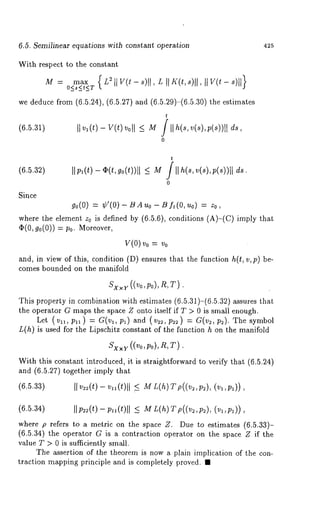
![426 6. Abstract Problems for First Order Equations
Consider now the case of a linear equation under the approved
decomposition of the function f:
(6.5.35) f(t, u,p) = L~(t) u + L2(t)p +
where for each fixed value t ¯ [0, T] the inclusions n~(t) L;(X),
£(Y; X) and f(t) ¯ occur. In thi s cas e a u ni que sol vability of the
inverse problem concerned is obtained on the whole segment [0, T].
Theorem 6.5.4 Let the closed linear operator A with a dense domain
generate a strongly continuous semigroup in the Banach space X, the op-erator
B satisfy condition (6.5.4), the inclusions uo ¯ "D(Are+l) and ¢ ¯
C1 ([0, T]; Y) and lhe compatibility condition Bu0 = ¢(0) hold. Let de-composition
(6.5.35) take place and the operator functions be such that
L~(t), ALI(t)A -1, Am+lnl(t) -m-1 ¯ C([0, T] ; £( X)),
Arn+lL2(t)g-m-1 ¯ C([0, T];£(Y; X)).
If, in addition, the function Arn+a f(t) C([0, T] ; X ), theoperator B Lu(t
is invertible for each 1 ¯ [0, T] and
(BL2) -a ¯ C([O, T]; £(Y)),
then lhe inverse problem (6.5.1)-(6.5.2) has a solution
u ¯ Ct([o,r];v(Am)) ~C([O,T];V(Am+t)), p ¯ C([0, T]; Y)
and this solution is unique in the indicated class of functions.
Proof The initial assumptions assure us of the validity of conditions (A)-
(E) with the ingredients
£(t,u) = n~(t) u + f(t),
f~(L u,V) = La(t)p,
fa(t,z,p) : B Lz(t)p,
¢(t,z) (-S~zL.y(t))
All this enables us to involve in the further development Theorem 6.5.3 and
reduce the inverse problem at hand to the system of the integral equations](https://image.slidesharecdn.com/0824719875inverse-141031173353-conversion-gate01/85/0824719875-inverse-447-320.jpg)
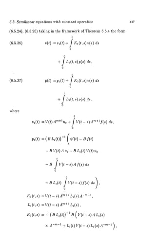
![6.5. Semilinear equations wi$h constant operation 429
this solution is unique in the class of continuous functions (see Section
5.1). This provides reason enough to conclude that the system (6.5.24),
(6.5.26) has a unique continuous solution on the whole segment [0, T] and
thereby complete the proof of the theorem."
Let us highlight a particular case of Theorem 6.5.4 with m = 0 in
which condition (6.5.4) admits an alternative form
(6.5.38) B ¯ £(X, Y).
This type of situation is covered by the following assertion.
Corollary 6.5.1 Let the closed linear operator A with a dense domain gen-erate
a strongly continuous semigroup in the Banach space X, the operator
B be in line with condition (6.5.38) and the relations Uo ¯ :D(A),
¢ ¯ c1 ([0, T];V ), BU o= ¢(0)
hold. When the decomposition
f(t, u, p) =- L, (t) u ÷ L~(t) p
is accepted with
L,, AL, A-~ ¯ 8([0, T]; £(X)),
AL~ ¯ C([0, T]; £(r, X)),
Afe C([0, T]; X),
the operator B L2(t) is invertible for each t [0, T] and
(Br ~)-’¯ C([0,T ];~ (Y)),
the inverse problem (6.5.1)-(6.5.3) has a solution
u ¯ 5q ([0, T]; X) ~ 5’([0, T]; ID(A)) p ¯ g([0, T]; Y)
and this solution is unique in the indicated class of functions.
In trying to apply the results obtained to partial differential equations
and, in particular, to the equation of neutron transport some difficulties
do arise in verifying the premises of Theorem 6.5.4 or Corollary 6.5.1. We
quote below other conditions of solvability of the inverse problem (6.5.1)-
(6.5.3) relating to the linear case (6.5.35) and condition (6.5.38).](https://image.slidesharecdn.com/0824719875inverse-141031173353-conversion-gate01/85/0824719875-inverse-450-320.jpg)
![43o 6. Abstract Problems for First Order Equations
Theorem 6.5.5 Lel the closed linear operator A with a dense domain gen-erate
a strongly continuous semigroup in the Banach space X, the operator
B satisfy condition (6.5.38), the inclusions uo E D(A), ~ C~([0, T] ; Y)
occur and the compatibility condition B uo = ~(0) hold. If the decomposi-tion
f(t,u,p) = L~(t)u+ L:(t)p+
lakes place wilh L1 ~ C1 ([0, T]; Z:(X)), Lz, A Lz ~ C([0, T];/~(Y, and
the function f = fl + f~, where
and
Is ~ c([0, N; V(A)),
the operator B L~(t) is inverlible for each t [0, T] and
(B L~)-1 e C([0, T]; £(Y)),
then the inverse problem (6.5.1)-(6.5.3) has a solution
u e c1([0, T]; x), p e c([0, T]; Y)
and this solution is unique in the indicated class of functions.
Proof Being concerned with the functions u ~ C~([0, T]; X) and p
C([0, T]; Y), we operate in the sequel with the new functi~Jns
F~(t) = L~(t) u(t), F~(t) : n~(t)p(O.
From the conditions of the theorem it seems clear that the inclusions
F, ~ 81([0, T]; X), Fe, AF~ ¢C([0, T]; X)
occur, due to which relations (6.5.1)-(6.5.2) ~re equivalent,
(6.5.39) u(t) = V(t) Uo V(t 8) f(s) ds
0
t
+ / v(t - ~) F~ (s)
0
+ / v(t - ~) F~(s)
0](https://image.slidesharecdn.com/0824719875inverse-141031173353-conversion-gate01/85/0824719875-inverse-451-320.jpg)
![6.5. Semilinear equations with constant operation 431
In what follows we deal with a new function
~o(t) = v(t) uo + / v(t - s) f(s)
0
In the" theory of semigroups the inclusion
rio(t) e 81 ([0, T]; X N C([0, D(A)
was established for any element Uo E D(A) and any function f = fl + f2
with the members fl E C1([0, T]; X) and f2 ~ C([0, T]; D(A)). Likewise,
using the well-known formulae of this theory we deduce the relationships
(6.5.40) A / V(t - s) F,(s)
0
= fv(t - s)r;(~) d~+V (t) r~(O)
0
(6.5.41)
t
V(t - s) F~(s)
0
= / V(t - s) A F2 (s)
0
In the derivation of the governing equation for the function p the operator
B applies to equation (6.5.1) with further reference to relation (6.5.35).
The outcome of this is
(6.5.42) ¢’(t) BAu(t)+BL,(t)u(t)+BL~(t)p(t)+Bf(t).
Calculating the values Au(t) and BL~(t) u(t) with the aid of relations
(6.5.39)-(6.5.41), substituting the resulting expressions into (6.5.42)
resolving the relevant equations with respect to the function p(t), we find](https://image.slidesharecdn.com/0824719875inverse-141031173353-conversion-gate01/85/0824719875-inverse-452-320.jpg)
![6.5. Semilinear equations with constant operafion 433
where
~o(t) = ( B L2(t))-l [ - BA~0(t
- B V(t) Ll(O)uo - Bf(t)]
K(t, s) = - ( B L2(t))-iB V(t L’I ( s),
L(t,s) = - ( S L~(t))-IB V(t - s)n,(s),
M(t,s) = - ( B L~(t))-l B s) A L2(s)
As equation (6.5.44) contains a derivative of the function u, there is a need
for enlarging the system (6.5.39), (6.5.44) by an equation u’, which
is obtained by formal differentiating of both sides of (6.5.39). Using the
general rules of differentiating
t / t
0
v(t - 8) ~(8) = V(t - 8),4 V~(8)
0
and excluding the nonintegral term F~(t) = L~(t)p(t) with the aid of
(6.5.44), we arrive
(6.5.45)
t
,~’(t)= Co(t+) / I~’(t,s ) ~(s)
0
t
+ / Zl(t,,)u’(,)
0
t
+f M~(t~, ) v(~)
0](https://image.slidesharecdn.com/0824719875inverse-141031173353-conversion-gate01/85/0824719875-inverse-454-320.jpg)
![436
(6.5.50)
6. Abstract Problems for First Order Equations
Comparison of (6.5.49) and (6.5.50) gives
(6.5.51) W,+l(t) u~+l(t ) = L~(t) (p ,+~(t) -p
t
+ / V(t- s)L~(s)(w~(s)
0
u~(s))
The sequence p~(t) converges to the function p(t) as n --~ oz uniformly over
the segment [0, T], so that the sequence
c,~ = sup L2(t) (p~+l(t) - p~(t))
te[0,T]
In conformity with (6.5.51) the norm of the difference
~.(t) = ~.(t) -
can be estimated as follows:
(6.5.5~)
t
0
where M is a positive constant. We claim that the sequence of functions
z~(t) converges uniformly to zero as n --* c~, Indeed, estimate (6.5.52)
being iterated yields the inequality
m-1
(6.5.53) II ~÷.~(t)ll (~M)
(mMr) + -- sup
m !](https://image.slidesharecdn.com/0824719875inverse-141031173353-conversion-gate01/85/0824719875-inverse-457-320.jpg)
![6.5. Semilinear equations with constant operation 437
Let e > 0. We choose the subscript k0 in such a way that for all k > k0 the
inequality
~ -MT
holds. Then
(6.5.54)
,~-1 (sMt)
E Ck+m-l-s
8!
~~ -MT ~ (MT) ~
-~7 -~ T - ~ s~-O
for all k _> ko and m _> 1. Holding a number mo fixed so that
(MT)msu p II"*o(t)ll ~
(6.5.55)
m ! ~10, T] ~
for all m > mo, we provide n = ko + m, m > too, as long as n > ko + too.
For this reason the bound
II r,~(t)ll = II r~o+m(t)ll < 7 + 7 =
is obtained for all values t ¯ [0, T] on the basis of (6.5.53)-(6.5.55).
this means that the sequence of functions r~(t) converges to zero uniformly
over the segment [0, T].
To complete the proof, we observe that the sequence of functions
u’~(t)= w~(t-) r~(t)
converges uniformly to w(t) as n -+ cx~, since the sequence w,~(t) converges
to the same function w(t) and the sequence rn(t) converges uniformly to
zero in both cases as n --~ o~. For this reason the function u(t) is differen-tiable,
u’(t) = w(t) and, in particular, u ¯ C1 ([0, T]; X). By inserting
L~ (s) u(s) = F~ L~(s)p(s) = F~(s)
and involving the explicit formula for ri0(t), equation (6.5.46) is transformed
into (6.5.39). Since the function u is continuously differentiable, we thus
have
e~ ¯ c’ ([0, T]; x); F~ , A F~ ¯ C([0, T]; X).
With these inclusions in view, relation (6.5.39) yields (6.5.1)-(6.5.2).
substituting u’ in place of w involved in (6.5.47) we come to (6.5.44).
guing in reverse order we see that relation (6.5.44) is followed by (6.5.43),
which is equivalent to (6.5.42) on account of (6.5.39). It is worth recalling](https://image.slidesharecdn.com/0824719875inverse-141031173353-conversion-gate01/85/0824719875-inverse-458-320.jpg)
![438 6. Abstract Problems for First Order Equations
here that formula (6.5.39) gives a solution ~f the Cauchy problem (6.5.1)-
(6.5.2). Because of (6.5.1), relation (6.5.42) becomes equivalent
equality
Su’(t) = ¢’(t),
which, in turn, is equivalent to
(Su(t))’= ¢’(t)
as far as the operator B is bounded. Further derivation of (6.5.3) is stipu-lated
by the compatibility condition B uo = ¢(0).
In accordance with what has been said, we conclude that if the func-tions
t~ e ~’1 ([0, T]; X) ~ ~’([0, T]; ~)(A)) p e c([0, rl; r)
give a solution of the inverse problem (6.5.1)-(6.5.3), then the triple
u~), p, w = u
is just a continuous solution of the system (6.5.46)-(6.5.48). Vice versa,
a triple of the functions
(u,p, w)
is a continuous solution of the system (6.5.46)-(6.5.48), then w = u’
the pair of the relevant functions (u, p) solves the inverse problem (6.5.1)-
(6.5.3). As stated above, the system of the integral equations (6.5.46)-
(6.5.48) has a continuous solution and this solution is unique. So, the
desired assertion of Theorem 6.5.5 follows immediately. ¯
6.6 Inverse problems with smoothing overdetermination:
quasilinear parabolic equations
Unlike the case of constant coefficients, the complete and uniform theory
for equations with variable operator coet~ieients is less advanced. In
trying to overcome some difficulties involved different approaches to various
wide classes of equations are offered. As in the theory of partial differen-tial
equations, in recent years the main objects of investigation were the
parabolic and hyperbolic types of abst_ract equations. Various equations
of parabolic type will be covered within the framework of the present sec-tion.
Readers who are interested in obtaining more detailed knowledge
of the general theory of abstract parabolic equations are advised to study](https://image.slidesharecdn.com/0824719875inverse-141031173353-conversion-gate01/85/0824719875-inverse-459-320.jpg)
![~.6. Quasilinear parabolic equations 439
Amann (1986, 1987), Fattorini (1983), Henry (1981), Krein (1967),
hata (1977), Sobolevsky (1961), Yosida (1965).
Let X and Y be Banach spaces. In what follows by A we mean a
mapping carrying out a subset from [0, T] × X into a class of closed linear
operators in the space X. It is supposed, in addition, that
f: [o, T] × X × Y ,-, X, B: [0, T] ~ ,C(.X, Y)
and
O: [O,T] ~ Y.
In such a setting we are looking for a pair of the functions
u ~ C~([0, T]; X), p e c([0, T]; Y),
satisfying the system of relations
(6.6.1) u’(t) = A(t,u(t))u(t)+f(t,u(t),p(t)), O<t<T,
(6.6.2) u(O) = u0,
(6.6.3) B(t) u(t) = ¢(t), o < t < T.
It is appropriate to mention here that the function u satisfies equation
(6.6.1) in a pointwise manner, meaning, in particular, that for any t
[0, T] the element u(t) belongs to the domain of the operator A(t, u(t)).
Relations (6.6.2) and (6.6.3) together imply a. necessary condition for
compatibility of the input data
(6.6.4) B(0) u0
Equation (6.6.1) is required to be of parabolic type, that is,
(P1) the closed linear operator A0 = A(0, Uo) has the dense domain ID,
the half-plane Rel >_ 0 is contained in the resolvent set of the
operator Ao and for any I with Re I _> 0 the inequality holds:
(Ao-~-l)~ <_l+ l,x---C--~.;
(P2) there are numbers ~ 6 (0, 1) and F~ > 0 such that for all u 6 X with
It u II-<- ~ anda ll t e [0, T] the linear dosed operator A(t, A;~u)
has the domain ID and there exists a constant fl 6 (0, 1) such that
for all t, s e [0, T] and all u, v e X with 1~ u ]1 ~ R and II v II ~ ~
the estimate is valid:](https://image.slidesharecdn.com/0824719875inverse-141031173353-conversion-gate01/85/0824719875-inverse-460-320.jpg)
![440 6. Abstract Problems for First Order Equations
[A(t, A;a u) - A(s, ~ v)] A~-I _<c ( It -8 [ ~ ÷[[ u - v [[ ).
The reader can encounter in the modern literature different definitions
of belonging to the parabolic class. This is due to the fact that different
methods are much applicable in investigating the Cauchy problem (6.6.1)-
(6.6.2). Commopnr actice involves the definition of Sobolevsky (1961)
so we adopt this definition in subsequent studies.
We impose the extra restrictions on ’the input data of the inverse
problem concerned:
(Pa) u0~, IIAgUoll < ~, ¢ ~ C~+e([0, T];~).
The operator B is subject to the following conditions:
(P4) for all t, s e [0, T] and all u, v e X with II ~ II ~ ~ ~.a II v II ~ ~
the operator B(OA (*, Ag%) Ag~ is bounded,t he estimate
(6.6.5) B(t) [A(t, ~ u)- A(s, Ag v)]
is true and
(6.6.6) B e C1+~([0, T]; £(X,Y)).
The boundedness of the operator
B(t) A(t, A-C~u) ~
ensures that the operator B possesses a certain smoothing effect similar
to (6.3.1). However, the requirement imposed above is more weaker than
the condition for the operator B A to be bounded.
As in Section 6.3 we may attempt the function f in the forrfi
(6.6.7) f(t,u,v) = fl(t, u) + f2(t,u,p).
The conditions playing here the same role as condi,tions (A)-(E) in Section
6.3 are as follows:
(P5) for the element
(6.6.8) zo= ~’(O)+B(O)Aouo-B(O)f~(O, Uo)-B’(O)uo](https://image.slidesharecdn.com/0824719875inverse-141031173353-conversion-gate01/85/0824719875-inverse-461-320.jpg)
![Quasilinear parabolic equations 441
the equation
B(O) f2(O, Uo,p)
with respect to p has a unique solution Po ¯ Y;
(P6) there exists a mapping fa: [0, T] x Y x Y ~-* Y, for which
B(t) f2(t,u,p) = fa(t, B(t)u,
(PT) for any fixed value * ~ [0, T] the mapping
has in the ball Sv(po, ~) the inverse
~ = ~(~,
all p, q ~ Yw ithI lv- poll5 ~ ~dI I q -poll~ ~ e~c ollectiono r
inequalities hold:
llk(*,Ag%)- k(< Ag%)l~l ~(I*- ° + II~- ~ll),
f=(,,~,q)[[
(pg) there is a number R~ > 0 such that for all *, s ~ [0, T] and all
mapping (6.6.9) obeys the estimate
II ~(*~, ,)- ~(*,z ~)[l5 ~ (l~- e + I ~, -
Theorem 6.6.1 Let conditions (6.6.7), (P1)-(P9) and (6.6.4) hold and
G < min{1-a,~3}.
Then there exists a number T1 > 0 such that on the segment.[O, T1] a
solution u, p of the inverse problem (6.6.1)-(6.6.3) exists and is unique in
the class of functions
~ ¯ c1([0,T 1];X ), p ¯ C~([0T, 1];V ).
Proof Involving the function p and holding the values T~ ¯ (0, T] and
K > 0 fixed, we are interested in problem (6.6.1)-(6.6.3). We denote](https://image.slidesharecdn.com/0824719875inverse-141031173353-conversion-gate01/85/0824719875-inverse-462-320.jpg)
![442 6. Abstract Problems for First Order Equations
by Q = Q/Ta,K,~) the set of all functions v ~ C~[0, T~]; X) for which
~(0) ~ A~ ~o and
II v(0 - ~(~)~I~ ~ I~ - ~,w, ~~ [0,~].
The set so constructed is closed and bounded in the space C([0, T~]; X).
The value T~ is so chosen as to satisfy the inequMity ~] v(t)l ~ ~ R for all
v ~ Q and all t ~ [0, T~]. This is certainly true if
~~ , < ((~-~;~0~)/~)
since the bound ~ v(0)~ < R is stipulated by condition (P3). On the
grounds as before, we define P = P(T~, K, ~) as the set of all functions
p e C([0, T~]; ~) for which p(0) : P0
~~,p(t)-p(s)~[ ~ K]t-s~ Vt, sG[O,T~],
It is possible to reduce the value T~ provided thut the inequality
~ ~(t) - ~0 ~ <
holds for all p ~ P and all t G [0, T~]. In dealin~ with the functions
v G Q, p G P we define the operator function
A(v;t) = A( t, ~ v( t))
and the function
F(v,p;t)= f(t, ~ v(t),p(t)).
Due to the boundedness of the operator A~-~ condition (PS) implies that
(6.6.10) F(v,p;t) - F(v,p;s)[_ < clt-where
the constant c does not depend on v E Q and p E P both.
The Cauehy problem related to the function u comes second:
f u’(t) = A(v;t)u(t)+F(v,p;t), 0<t<T1,
(6.6.11) u(0) = u0.
It is well-known from Sobolevsky (1961) that for a sufficiently small value
T1 > 0 and any v ~ Q the operator function A(v; t) generates an evolution
operator U(v;t, s) being strongly continuous for all 0 _< s < t < Ta. A](https://image.slidesharecdn.com/0824719875inverse-141031173353-conversion-gate01/85/0824719875-inverse-463-320.jpg)
![6.6. Quasilinear parabolic equations 443
solution of problem (6.5.11) in the class u ~ 1 ([0, T 1]; X) exists an d is
given by the formula
(6.6.1~) u(t) = u(v;~,0)u0+/ ds.
o
Furthermore,
(6.6.13) [A~[U(v;t,O)-U(v;s,O)]A; I <_ 1C-]~~--8[
and for any function F 6 C([0, TI]; X) ~he es~ima%ei s true:
~+~
0 0
< c~t~l-~(~log~&¢~+l) max ~F(~)~.
What is more,
(6.6.1~) I1~ g(v;~,~)~l ~ ~ - -~,
Here the constant c is independent of v ~ ~ (for more detail see Sobolevsky
(1961)). Recall once again that ~he same symbol c may stand for different
constants in later calculations.
It is also a matter of the general experience that for a su~ciently small
value T~ there exists in the class ~ a unique function depending, in general,
on p and providing the same solutions to both problems (6.6.1)-(6.6.2)
(6.6.11). It w~ shown in Sobolevsky (1961) that u(~) ~ v(~)
Holding the function v fixed we are going to derive the governing
equation for another Nnction p. By virtue of conditions (6.6.4) and (6.6.6)
relation (6.6.a) is equivalent to
(~.~.~ ~(~ ~’(~ + ~’(~) ~(~ = ~’(~).
In turn, (6.6.1), (6.6.12) and (6.6.7) are followed
(6.6.17) B(¢) u’(¢) = B(~)(I(Lu(~),p(~)) - A(~,u(~))u(~))
- ~(~)~ (v;~ ~(v;~ , 01~ 0- ~(~~ (~;
ds.
o](https://image.slidesharecdn.com/0824719875inverse-141031173353-conversion-gate01/85/0824719875-inverse-464-320.jpg)
![444
6. Abstract Problems for First Order Equations
Likewise, (6.6.12) implies that
(6.6.18) B’(t) u(t) = B’(t) (U(v;t,O)
t
0
To make our exposition more transparent and write some things in simpli-fied
form, it is convenient to introduce the notations
w(t) = A~U (v;t,O)uo+ A~f tU(v;t,s)F(v,p;8)
o
a(v,t) = ¢’(t) B(t) fl (t, A; ~v(t)),
D(v; t) = B(t) A(~; t) Ag~ - ~’(t) ~,
z(t) = a(v;t) + D(v;t)
Substituting (6.6.17) and (6.6.18) into (6.6.16)
(6.6.19) B(t) f~(t, u(t),p(t))
The increment of the function z can be evaluated as follows:
(6.6.20) II z(t) - z(s)lI <_ II a(v; t) - a(v; I
+I I D(v; t) - D(v; ~)1’1 II ~(t)II
£rom the definition of the function a(v; t) it follows that
II a(~; ~) - ~(~; 8)11 < II V(~) - ~’(~)11. ÷ II
× II .fl (t, A~~ ~(t))- f~( ~, -~~ (~))II.
Since v G Q, the inequality IIv(t)ll < Rholds true for any t G [0, T~].
Therefore, under condition (P8) there is a constant M > 0 such that for
all t G [0, Ta] and all v ~ Q the estimate
I[£(t, A~ v(t))[I <_](https://image.slidesharecdn.com/0824719875inverse-141031173353-conversion-gate01/85/0824719875-inverse-465-320.jpg)
![6.6. Quasilinear parabolic equations 445
is valid. A proper choice of the constant M (enlarged if necessary) provides
the validity of the inequality
II B(t)ll -<
for all* E [0, T~]. By conditions (P3), (6.6.6) and (P8),
(6.6.21) ]]a(v;t)-a(v;s)[ I < c]t-s]a +c M]t-sl
+c (It- + II v(t) - v(s)ll)
From the definition of/)(v; t), conditions (P4) and (6.6.6)in combination
with the boundedness of the operator Aj= we deduce that
(6.6.22) D(v;t)- D(v;s)
For any v ~ Q, p G P the value F(v,p;O) = f(O,uo, po) and (6.6.10)
together imply the existence of a constant M > 0 sudi that for any v
Q, p G P and all t G [0,
Since u0 G D, we are led by relations (6.6.13) ~nd (6.6.14)
(6.6.23) llw(t+At)-w(t)[] IAtt ~-=l[Aouoll+c M
Keeping ~ < 1 - ~ and letting ~ ~ ~ 0, it is not diNcult to establish the
asymptotic relation
which is uniform in v ~ 0, P ~ P and over the segment ~
thermore, by the definition of the %notion w we establish the relationship
~(0~ =
thereby clarifying that the Nnction w belongs to Q for a su~ciently small
number T~ and any v ~ Q, p ~ P.
In the current situation ghe action of the operator A~ with respect
relation (6.6.12) leads to the equation for the Nnction
(6.6.24) v(~)](https://image.slidesharecdn.com/0824719875inverse-141031173353-conversion-gate01/85/0824719875-inverse-466-320.jpg)
![446 6. Abstract Problems for First Order Equations
Observe that z(0) = z0, where the element z0 is defined by (6.6.8). Inserting
the value s = 0 in (6.6.20) and taking into account (6.6.21)-(6.6.22),
arrive at
whenT I is smalle nougha ndb othe lementvs and w belongt o (~. By virtue
of~ ump~io(nP~ )-(~PqT.)~ i(o~n. ~.¢~~)n b ~~
(6.6.25) p(t) = O(t, z(t))
The desired assertion will be proved if we succeed in showing that the sys-tem
(6.6.24)-(6.6.25) possesses in Q x P a unique solution for a sufficiently
small value T1. This can be done using the function
g(t) = q~(t, a(w;t) + D(w;t)w(t)).
It is straightforward to verify that g(0) : P0. Moreover, condition (P9)
implies the estimate
(6.6
II g(t)g (~)ll _e< (It- ~z +I t ~w( ;t ) - a(w; s)lI
+ [ID(w;t)- D(w;s)ll II w(t)l[
Using estimate (6.6.22) behind we deduce that there is a constant M >
for which the inequality
IID(w,t)ll < M
holds true for any w 6 Q and all t 6 [0, T1]. By successively applying
inequalities (6.6.21)-(6.6.22) with w standing in place of v and relying
(6.6.26), we find that
It g(t) g(s)ll < c (It - s z .÷I I w()t - w(s)ll)
with a positive constant c > 0. Since ~ < fl, the existence of a sufficiently
small value T~ such that the function g belor~gs to P is ensured by the
preceding inequality in combination with (6.6.23).
At the next stage the metric space Q x P is equipped with the metric
~ induced by the norm of the space C([0, TJ; X ) x C([0, T~]; Y ), making
it possible to introduce in this space the operator
a: (v, p) ~ (w,](https://image.slidesharecdn.com/0824719875inverse-141031173353-conversion-gate01/85/0824719875-inverse-467-320.jpg)
![6.6. Quasilinear parabolic equations 447
As we have mentioned above, the operator G carries out Q x P into itself
if the value T1 is sufficiently small.
As can readily be observed, the solutions of the system (6.6.24)-
(6.6.25) coincide with the fixed points of the operator G.
Let vl, v2 E Q; pl, p2 E P and
Putting these together with the relationships ul = A~-ow~ and u2 =
A~"~ w~ we derive the system
(6.6.27) {u~(t) A(v~;t) u~ (t)+ F( v~,p~;t),
u’~(t) = A(v~ ;t) u~(t) + F(v~, p~;
supplied by the condition ua(0) = u2(0) = u0. Whence it follows that
function u = ul - u2 solves the Cauehy problem
(6.6.28) f = A(v ;t) + F(t), 0 < t = o,
with F(t) = [ A(v~;t) - A(v~;t)] u2(t) + F(v,,p~;t) - F(v~,p~;t) incorpo-rated.
By condition (P2) and the definition of Q the function
A(t) = [A(v=;t)- A(va;t)] IAj
happens to be of HSlder’s type in the space £(X) with exponent (r and
constant not depending on vl, v2 ~ Q..
On the other hand, estimates (1.71) and (2.27) from Sobolevsky (1961)
could be useful in the sequel if they are written in terms of problem (6.6.27).
With these in view, inequality (6.6.10) clarifies that the function A0
is of H61der’s type for t > 0 and is unif6rmly bounded with respect to
v2 ~ Q, p~ ~ P, t ~ [0, T~], that is,
(6.6.29) 11Aou~(t)[[ <~ M.
Therefore, a solution of the Cauchy probleh~ (6.6.28) can be represented
via the evolution operator (for more detail see Sobolevsky (1961))
t
(6.6.30) u(t) = / U(va;t,s) F(s)
0](https://image.slidesharecdn.com/0824719875inverse-141031173353-conversion-gate01/85/0824719875-inverse-468-320.jpg)
![6. Abstract Problems for First Order Equations
We are led by assumption (P2)
(6.6.31) I{ A(t)l] <- c II v2(t) Iv.l (t)l
In turn, the combination of (6.6.7) and (P8) gives the inequality
(6.6.32) IIF(vl,pl;t)-F(v2,p~;t)ll _<c(2 live(t)-v~(t)ll
+ 11p2(t)
Applying the operator A~ to (6.6.30) with further p~ssage to the appropri-ate
norms we deduce with the ~id of (6.6.15), (6.6.29) ~nd (6.6.31)-(6.6.32)
that
t
0
+ c (~ ~ ~(t) - ~(t)~l + ~ ~(t) - ds.
This provides reason enough to conclude that there is a positive constant
c~ > 0 such that
(6.6.33) II ~1w I~IC(~O,T,~;X~) ~ ~?-~ P((’~,P,), ,(P~~)) ,
where p refers to a metric of the space Q x P.
By ~ssumption (Pg), the following estimate
IIg~(t)- g~(t)ll~ c( lla(w~;t)a=( w=;t)ll
+ ~ D(w,;t-) D(w~;t)ll
+ ~ D(~;t)i¯] ~l w~(t)
is ensured by the definition of the function g. By virtue of condition (P8)
we thus have
while condition (P4) impfies that
[I o(~; t) - O(w~;t)~ll ~ ~ ~(t) ~(t)]l.
From the inclusion wa ~ Q it follows that ~ w~(t)l I < R. The estimate
(6.6.34) ~lga --9~C([O,Ta];Y) ~ c~ T~-~ p((va,p~), (vz,p~))
c~n be justified by the uniform boundedness of the operator functions
D(w~,t) and B(t) ~nd the preceding estimate (6.6.33). Here e~ > 0
u positive constant. On the basis of estimates (6.6.33)-(6.6.34) we
clude that the operator G is contractive in Q x P if Ta is sufficiently small.
This completes the proof of the theorem. 1](https://image.slidesharecdn.com/0824719875inverse-141031173353-conversion-gate01/85/0824719875-inverse-469-320.jpg)
![6.6. Quasilinear parabolic equations 449
6.7 Inverse problems with singular overdetermlnation:
semilinear parabolic equations
In this section we consider the inverse problem (6.6.1)-(6.6.3) in the
when equation (6.6.1) is semilinear. The appropriate problem statement
is as follows:
(6.7.1) u’(t) = A(t) u(t) + f(t, u(t),
O<t<T,
(6.7.2) u(0) = Uo,
(6.7.3) B ~,(t) = ¢(t), 0 _< <,T.
Here the operator B is supposed to be bounded from the space X into the
space Y and (6.7.3) is termed a singular overdetermination. The pres-ence
of (6.7.1) in the class of parabolic equations is well-characterized
by the following condition:
(PP1) for anyt E [0, T] the linear operator A is closed in the space X and
its domain is dense and does notdepend on t, that is,
7)(A(t))
Also, if A is such that ReA >_ O, then for all t ~ [0, T] and A ~
p(A(t))
C
(A(t)-AI)-I <-IAI+I’
where c is a positive constant.
Further treatment of the inverse problem concerned necessitates in-volving
the well-posedness of the direct linear problem
(6.7.4)
u’(t) A(t) u( t)+f(t),
u(0)=Uo.
O<t<T,
Granted (PP1), a sufficient condition for the direct problem (6.7.4) to
well-posed is as follows:
(PP2) there exist a constant c > 0 and a value ~ ~ (0, 1] such that for all
t, s, v ~ [0, T] the inequality holds:
IliA(t)-A(s)] ~A.-~(r) <_ c It-sl](https://image.slidesharecdn.com/0824719875inverse-141031173353-conversion-gate01/85/0824719875-inverse-470-320.jpg)
![450 6. Abstract Problems for First Order Equations
Under conditions (PP1)-(PP2) the direct problem (6.7.4 has a strongly
continuous evolution operator in the triangle
~(T)= {(t, s): 0 ~ s < T, 8 < ~ <
If each such case u0 E /3 and the function f is subject to either of the
following conditions: A f E C([0, T]; X) or f is of HSlder’s type in the
space X, then problem (6.7.4) has a unique solution u ~ C~([0’, T]; X),
this solution is given by the formula
t
(6.~.~) ~(t) u(t, o)~o + /u(t,~) f( ds
o
and the operator function
W~ (t, s) = A(t) U(t, s)
is strongly continuous in A(T). What is more, the function
Wl+~(t,s) = AI+~(t) U(t,s)A-I-~(s)
will also be strongly continuous in A(T) for ~ < a. If one assumes,
~ddition, that u0 ~ 9(A1+~(0))
~+’(t)f (t) c([0, ~]~ x)
then a solution of problem (6.7.4) will comply with the inclusion
(6.~.6) ~’(0)~(t) e cl([0, ~];
We refer ~he reader to Sobolevsky (1961).
Let the operator B meet one more requirement similar in form to
(5.1.~):
(6.7.7) ~ ~ ~(9(~(0)), ~ < ~,
where the manifold ~(A~(0)) is equipped with the
~~ ~ , =~ 1~ ’(0~) .
On the same ~rounds as before, we may attempt the function f in the form
(6.7.s) f(t, ~,p)= f ~(t,~ )f ~(t, ~;,).](https://image.slidesharecdn.com/0824719875inverse-141031173353-conversion-gate01/85/0824719875-inverse-471-320.jpg)
![6.7. Semilinear parabolic equations 451
With the aid of relations (6.7.6)-(6.7.7) it is not difficult to show that
two conditions
(6.7.9) ~ E C1([0, T]; Y), Bu0 = ~(0)
are necessary for the solvability of the inverse problem (6.7.1)-(6.7.3)
the class of functions
u E C1([0, :~]; X),
By means of the functions ~b E C1([0, T]; Y) and u0 ~D(BA(O)) we
define the element
(6.7.10) Zo = ~b’(0) B A(O) Uo- B f~(O, Uo)
and involve it in the additional requirements:
(VV3) the equation B f~(O, uo,p) = Zo with respect to p has a unique
solution Po ~ Y;
(PP4) there exists a mapping
f3: [O,T]xYxY ~--* Y
for which
(6.7.11) B fz(t,u,p) = fz(t,Bu,p)
(PP5) there is a number R > 0 such that for any t ~ [0, T] the mapping
z = fz(t, ~b(t),
has in the ball Sy(po, R) the inverse
(6.7.1~) p = ~(t,z).
With the relation u0 ~ 7)(A1+~(0)) in view, the following manifolds
SI ( R, T) = { ( t, z, p): O <T, Il z - A(O) uo ll < Rlip -poll <R},
So(n,r ) = {(t,z,;): 0 <~< T,I Iz-uoll< 2, lip- ;oil <
SI+~(n,T) = {(t,z,p): 0 < t < T, Ilz- AX+fl(O)uoll < n,
II;-;oll < n}](https://image.slidesharecdn.com/0824719875inverse-141031173353-conversion-gate01/85/0824719875-inverse-472-320.jpg)
![452 6. Abstract Problems for First Order Equations
are aimed to impose the extra smoothness restrictions:
(PP6) there is a number R > 0 such that for k = 0, 1,/3 + 1 either of th’e
functions
Ak(t)fl(t, A-k(t)u)
and
A~(t) f2( t, A-~(t)u,
is continuous with respect to the totality of variables and satisfies
on the manifold S~(R,T) the Lipschitz condition with respect
(PP7) the mapping (6.7.12) is continuous on the set Sy(ZO, R,T) and
satisfies thereon the Lipschitz condition in z.
Theorem 6.7.1. gel conditions (PP1), (PP2), (6.7.7) and (6.7.9) hold. If
u0 e :D(AI+Z(0)) and conditions (6.7.8), (PP3)-(PP7) are valid with
element zo given by formula (6.7.10), then there is a value TI > 0 such that
on the segment [0, T~] a solution u, p of the inver.se problem (6.7.1)-(6.7.3)
exists and is unique in the class of functions
u e CI([O,T~];X), Au C( [0, T~ ];X), )p.eC([O, Td;Y
Proof By assumption, the inclusions
p e C([0, T]; V
and
v(t) = A(t) u(O C([0, T] ; X
imply that the superposition
fl(t) = f(t, A-l(t) v(t),
is continuous. The same remains valid for the function A(t) fl (t). If so, the
Cauchy problem (6.7.1)-(6.7.2) will beequivalent to the integral equation
t
(6.7.13) = U(t,s) f( s,u(s),p(s)) ds
0
in the class of functions u e C([0, T]; X ) for which the inclusion
e C([0T, ]; X)](https://image.slidesharecdn.com/0824719875inverse-141031173353-conversion-gate01/85/0824719875-inverse-473-320.jpg)
![6.7. Semilinear parabolic equations 453
occurs. Indeed, a solution to equation (6.7.1) complies with the condition
Al+~(t)u(t) C([0, T] ; X)
if the value T is sufficiently small. To make sure of it, we first perform the
substitution z(t) = AI+Z(t) u(t) with
zo(t) = A~+Z(t) U(t,O) uo = W~+~(t,O)
thereby justifying that the function u satisfies the integral equation (6.7.13)
if and only if the function z solves the integral equation
(6.7.14)
t
z(t) = Zo(t) + f w,+z(t,s)g(s,z(s),p(s))
o
where
g(t, z,p) = A’+~(t) f( t, A-~-O(t)
It is worth noting here that z0 is continuous on the segment [0, T] and
the kernel WI+~ is strongly continuous on the set A(T). Moreover,
condition (PP6) the function g is continuous and satisfies the Lipschitz
condition in z. This serves to motivate that equation (6.7.14) has a unique
local solution in the class of continuous functions. Reducing the value T,
if necessary, one can accept (6.7.14) to be solvable on the whole segment
[0, T]. Recall that T may depend on the function p.
Due to the interrelation between solutions to equations (6.7.13) and
(6.7.14) the function
f(t) = f(t, u(t),
satisfies the equality
A~+~(t) f(t) = AI+Z(t) f(t, A-~-Zz(t), p(t))
and is continuous on the strength of condition (PP6). In view of this,
solution of the Cauchy problem (6.7.1)-(6.7.2) obeys (6.7.6). Because
(6.7.7),
(B u(t))’
so that relation (6.7.3) is equivalent to the following one:
Su’(t): ¢’(t), 0<t<T,
making it possible to reduce the preceding on the basis of (6.7.1)
(6.7.15) p(t) = ¢;(t,¢’(t)- BA(t)u(t)- B fl(t,u(t))).](https://image.slidesharecdn.com/0824719875inverse-141031173353-conversion-gate01/85/0824719875-inverse-474-320.jpg)
![454 6. Abstract Problems for First Order Equations
Here we have taken into account conditions (6.7.8), (PP4) and (PPh).
By involving formula (6.7.13) and substituting z(t) = l+z (t)u(t) we
are led to an alternative form of wriiting (6.7.15):
(6.7.16) p(t) = 0~ t, go(t)+gl(t,z(t))+ K(t,s)g(s,z(s),p(s))
o
where
Since
go(t)= ¢’(t)- BA (t)U (t,Ou)o - Bf ~(t , U(t,O)
g~(tz, ) ~-- -B( fl(t, A-~-Z(t) z ) fl( t, U(, tO)u o) )
I(.(t, s) -BA(t) U(t , s) A-I-Z(s),
g(t, z,p) = A~+Z(ft()t ,A-l-O(t)z,p).
B A(t) U(t, O) uo = A-~(0)) (A~( A-~(t))
× A~+ZU(t()t ,~ o
= ( B A-/~(O)) (AZ(O)A-Z(t))
× W~+~(t,O)(A’+Z(0)u0) ,
the function go(t) C([0, T] ; Y) . This is dueto t he fact that the f unction
A~ (0)A-~ (t)is strongly continuous (see Sobolevsky (1961)). Also,
attempt the function g~(t, z) in the form
gl (t, z) = ( B A-0 (0)) z (0)A-8 (t))
x (A~+~(t) f~(t,A-~-~(t)z)
- A~+~ (t) fl (t, -~-~ (t)
x Wl+~(t, 0) AI+~(0) u0)),
implying that the function g~ is continuous with respect to the totality of
variables and satisfies the Lipschitz condition in z. Likewise, the kernel
K(t, s) admits the form
I((t, s) -= -(B A-Z(0)) (AZ(0) A-Z(t)) W~+z(t,](https://image.slidesharecdn.com/0824719875inverse-141031173353-conversion-gate01/85/0824719875-inverse-475-320.jpg)
![6.7. Semilinear parabolic equations 455
thereby justifying the strong continuity of I((t, s) in A(T)..
Thus, the system of the integral equations (6.7.14), (6.7.16) is derived.
Observe that it is of some type similar to that obtained ir~ Section 6.3 for
the system (6.3.9), (6.3.12). Hence, exploiting some facts and adopting
well-developed tools of Theorem 6.3.1, it is plain to show that the system
(6.7.14), (6.7.16) is solvable, thereby completing the proof of the theorem.
Of importance is the linear case when
(6.7.17) f(t, u, p) = L1 (t) u + L~(t)p +
Theorem 6.7.12 Lel condilions (PP1)-(PP2), (6.7.7) and (6.7.9)
Uo G V(AI+/)(0)), the operator functions
L1, ALl A-1IAI+~ L1 a -1-e e C([0,
AI+eLe C2 ([0T, ];e (r, x))
and the function
~*+~~ e c([0, r]; x).
if for any t ~ [0, T] the operator B L~(t) is invertible in the space Y and
(~n ,)-~e C([0,r ]; ;(r)),
then a solution u, p of the inverse problem (6.7.1)-(6.7.3), (6.7.17) exists
and is unique in the class of functions
~ e c~ ([o, r]; x), ~ e c([0, ~]; x), v e c([0, r];
Proof By virtue of conditions (PP3)-(PPT) with the ingredients
f~(t,u) = n~{t) u + F(t),
k(t,z,v) ~n~(t)~,
-¢~(t, z) (~ L~(t)) ~ Z](https://image.slidesharecdn.com/0824719875inverse-141031173353-conversion-gate01/85/0824719875-inverse-476-320.jpg)
![456 6. Abstract Problems for First Order Equations
one can recast the system of equations (6.7.14), (6.7.16)
t
(6.7.18) z(t) :zo(t) +/(I~_’l(t,s)z(s) +Ll(t,s)p(s))
o
(6.7.19)
where
t
p(t) = Po (t) + / ( K~ (t, s) z(s) + L~ (t, s)
0
zo(t) = I/Vl+~(t, 0)Al+~3(0)
t
+ / Wl+/3(t, s) Al+f3(s) F(s) ds,
0
Kl(t, s) = Wl+~(t, s) (Al+~(s) nl A-l- ~(s)) ,
Ll(t, ~)= W l+~(st), ( A~+e(Ls~) (~))
po(t) = (BL~(0-~) [¢’(0 - Br(t)
- B A(t) U(t, O) uo - B.L1 (t) U(t, Uo
t
- B A(t) / U(t, s) r(s) ds
0
t
0
I(2 (t, s) = - ( B L2 (t))-i [ B A(t) U(t,
× A-~-Z(s) + B L~(t)A-~-Z(t)W~+~(t,s)
× AX+e(s) Ll(s) A-l-Z(s)]
L:(t,s) = - ( B L2(t))-’ [ B A(t) U(t,s)
+ B L,(t) m-i-Z(t) Wl+e(t, s) A~+Z(s) L:(s)]](https://image.slidesharecdn.com/0824719875inverse-141031173353-conversion-gate01/85/0824719875-inverse-477-320.jpg)
![458 6. Abstract Problems for First Order Equations
6.8 Inverse problems with smoothing overdetermination:
semilinear hyperbolic equations
As in Section 6.7 it is required to find the functions u ¯ C1 ([0, r]; X ) and
p ¯ C([0, T]; Y) from the set of relations
(6.8.1)
u’(t) = A(t)u(t) + f(t, u(t),p(t)),
O<t<T,
(6.8.~)
u(O=) uo,
(6.8.3)
B u(t) = ¢(t), 0 < t < T.
For any t ¯ [0, T] a linear operator A(t) with a dense domain is supposed
to be closed in the space X. The symbol B designates a linear operator
acting from X into Y and
f: [O,T]xXxY ~ X.
Much progress in investigating the inverse problem (6.8.i)-(6.8.3) is
nected with the subsidiary information that the linear direct problem
(6.8.4) u’(t) = A(t) u(t) +
O<t<T,
(6.8.5) u(0) = uo,
is well-posed.
Before proceeding to a more detailed framework, it is worth noting
here that the reader can encounter in the modern literature several different
definitions and criteria to decide for yourself whether equation (6.8.1) is
hyperbolic type. Below we offer one of the existing approaches to this .issue
and take for granted that
(Ill) /’or any t ¯ [0, T] the operator A(t) is the generator of a strongly
continuous semigroup in the space X;
(H2) there are constants M and ~3 such that for any A > ~3 and any finite
collection of points 0 <_ tl <_ t~ <_ .. <_ tk <_ T the inequality holds:
( A(tk) - A -1 ( A(tk_~) - A I) -1 ’’ ’
M
A(t,)-AI) -1 <_ ()~_~)~](https://image.slidesharecdn.com/0824719875inverse-141031173353-conversion-gate01/85/0824719875-inverse-479-320.jpg)
![6.8. Semilinear hyperbolic equations 459
One assumes, in addition, that there exists a Banach space X0, which
can densely and continuously be embedded into the space X. In this view,
it is reasonable to confine yourself to particular cases where
(H3) there exists an operator function S(t) defined on the segment [0, T]
with values in the space 12( Xo, X ); this function is strongly contin-uously
differentiable on the segment [0, T] and for any fixed value
~ E [0, T] the operator
[s(t)]-’ ¯ t(x,
and
S(t) A(t) [ S(t)] -1 A.(t) + R(t),
where R(t) ¯ £(X) and the operator function R(t) is strongly
tinuous in the space X;
(H4) for anyt ¯ [0, T] the space Xo C :D(A(t)) and the operator function
A ¯ C([0, T]; £,(Xo, X)).
Under conditions (H1)-(tt4) there exists an evolution operator
U(s,t), which is defined on the set
A(T) = {(t,s): O<s<T,s<t<T}
and is strongly continuous on A(T) in the norm of the space X. By means
of this operator a solution u of problem (6.8.4) is expressed
(6.8.6)
t
u(t) = U(t, O) Uo +’/ U(t, s) f(s)
0
For u0 ¯ X and f ¯ C([0, T]; X) formula (6.8.6) gives a continuous solu-tion
(in a sense of distributions) to equation (6.8.1) subject to condition
(6.8.2). Furthermore, with the inclusions u0 ¯ X0 and f ¯ C([0, T];
in view, the preceding formula serves ~’or a solution of the Cauchy problem
(6.8.1)-(6.8.2) in the class of functions 1 ([0, T ]; X) (f or more de tail se
Fattorini (1983), Kato (1970, 1973), Massey (1972)).
The present section devotes to the case when the operator B possesses
a smoothing effect, meaning
(6.8.7) B ¯ 12(X, Y), B A ¯ C([0, T]; 12(X, Y)).](https://image.slidesharecdn.com/0824719875inverse-141031173353-conversion-gate01/85/0824719875-inverse-480-320.jpg)
![460 6. Abstract Problems for First Order Equations
Now our starting point is the solvability of the inverse problem (6.8.1)-
(6.8.3) in the class of continuous functions. Omitting some details, a con-tinuous
solution of the inverse problem concerned is to be understood as a
pair of the functions
u ¯ g([O, T]; X),
satisfying the system of relations
(6.8.8) ~,(t) U(t, O)
t
+ f u(t, 8)
0
p ¯ C([0, T]; Y),
s,u(8),p(8)) ds, 0 < t < T,
(6.8.9) Bu(t) =¢(t), 0 < t <
The approved decomposition
(6.8.10) f(t,u,v) = f~(t,u)+ f~(t,u,p)
will be used in the sequel. Allowing the element ¢ to be differentiable at
zero we define the element
(6.8.11) zo = t/,’(0)- B A(O) % - B f~(O,
and assume that
(Hb) the equation B ~(O, uo,p) = Zo ~¢ith respect to p has a unique
solution Po ¯ Y;
(H6) there exists a mapping f3: [0, T] x Y x Y ~ Y such that
(6.8.12) B f2(t,u,p) = f3(t, Bu,p);
(H7) there is a number R > 0 such that for any t ¯ [0, T] the mapping
z = f3(t, ¢(t),p) has theball Sy(po, R) th e i nverse
(6.8.13) p = ~(t,
In addition to the algebraic conditions (Hb)-(HT), we impose the extra
smoothness conditions:
(HS) there is a number R > 0 such that either of the functions fl(t, u)
and f2(t, u, p) is continuous with respect to the totality of variables
and satisfies on the manifold 5’Xxv ((Uo,Po), R,T) the Lipschitz
condition with respect to (u,p);
(H9) there is a number R > 0 such that the mapping (6.8.13) is con-tinuous
with respect to the totality of variables and satisfies the
Lipschitz condition in z on the manifold Sv (Zo, R, T), where the
element Zo is defined by (6.8.11).](https://image.slidesharecdn.com/0824719875inverse-141031173353-conversion-gate01/85/0824719875-inverse-481-320.jpg)
![6,8. Semilinear hyperbolic equations 461
Theorem 6.8.1 Let conditions (6.8.7), (6.8.10), (H1)-(H9) hold and Uo ¯
X, ¢¯CI([0,T];Y) and Buo =¢(0). Then there is a value Ta > O such
lhal on the segment [0, Ta] a solution u, p of the inverse problem (6.8.1)-
(6.8,3) exists and is unique in the class of continuous functions
~ ¯ c([0, T]; x), p ¯ C([0, T]; Y).
Proof By the initial assumptions the function
(6.8.14) f(t) = f(t,u(t),p(t))
is continuous on [0, T] for arbitrary fixed functions u ¯ C([0, T]; X) and
p ¯ C([0, T]; Y). Within notation (6.8.14), the definition of the solution
of the inverse problem (6.8.8)-(6.8.9) is involved in the further derivation
of the equation
(6.8.15) ¢(t) = B U(t, O) uo + B J U(t, s) f(s)
0
In the sequel we shall need yet two assertions to be proved.
Lemma 6.8.1 For any element Uo ¯ X and all values t >_ s lhe function
is differentiable and
¢0(t) = u(t, s)
¢~(t) = B A(t) U(t,s)
Proof Recall that the subspace X0 is dense in the space X. Hence there
exists a sequence of elements un from the space X0 converging to an element
u0 in the space X. Set
¢~(t) = B V(t,s)
and appeal to the well-known estimate for the evolution operator
IIU(t,s)] I <_ M exp(/?(t-s)).
The outcome of this is
II ¢,~(t-) ¢o(t)l<l _M I I BI I exp(I Zl T)I I](https://image.slidesharecdn.com/0824719875inverse-141031173353-conversion-gate01/85/0824719875-inverse-482-320.jpg)
![462 6. Abstract Problems for First Order Equations
implying that the sequence of functions ~b~ converges as n -~ cx~ to the
function ~bo uniformly over Is, T]. Since un E Xo, the function ~bn is differ-entiable
on the segment Is, T] and
~b’~(t) = BA(t)U(t,s)u~ = BA(t) V(t,s)u~,
whence it follows that
~(t) ~ ~(t) = B A(t) U(t,
~ n ~ ~. On the basis of the estimate
II G(t)~ (t)[I ~s up ItB (At) II Me xp([ f l[ T) ~1 u~ -u0 ~l
[0,T]
we deduce that the preceding convergence is uniform over the segment
Is, T]. Becauseo f this fact, the function ~o is differentiable and ~ = ~,
which completes the proof of the ]emma.~
~e=m~ ~.S.: ~t f ~ C([0, ~]; X ) a,~
t
~(~) = u / u(~, ,)f(,) ds.
0
Thent he [unction g is di~erentiable on the segmen[t0 , T] and
t
a’(t) = ~ A(t) / U(t, ~) I(,) & +
0
Proof From the additivity of integrals it follows that
t+h (~.s.l~)~(t + ~) - ~(t) 1 f ~ = ~~ u u(t + ~, ,) ~(,)
t
t
+ [ ~ u(t + ~, ~) - g(t, ,) [(s)d s.
0
Since
1](https://image.slidesharecdn.com/0824719875inverse-141031173353-conversion-gate01/85/0824719875-inverse-483-320.jpg)
![6.8. Semilinear hyperbolic equations 463
and the function H(t, s) = U(t, s)f(s) is uniformly continuous in the tri-angle
A(T), the first term on the right-hand side of (6.8.16) converges
B f(t) as h --~ 0.
The next step is to show that the limit as h --~ 0 of the second term
on the right-hand side of (6.8.16) is equal
t
B A(t) / U(t,
0
ds.
This fact immediately follows from the relation
t t
(6.8.17) lim gh(S) ds = / go(s
0 0
where
gh(~)= U t( + h,s) - U(t, s)
h f(s),
go(s) = B A(t) U(t,s)
First of all observe that by Lemma6 .8.1 the function go(s) is a point-wise
limit of the functions gh(s) as h -~ on[0, T]. Therefore, rela tion
(6.8.17) will be established if we succeed in showing that the norms
these functions are uniformly bounded. This can be done using the func-tion
#~(t) = B U(t, s) f(s) of the variable t. By Lemm6a .8.1,
#~s(t) = B A(t) U(t, s) f(s)
By the same token,
gh(~,)~ (t +h )- ,~(t)
h
and, in agreement with the mean value theorem,
I #~(t + h)- p~(t)
(6.8.18) Ilgh(s)ll----I < sup
h - [o, T]
On the other hand, #~s(t) as a function of two independent variables is
continuous in A(T) and thus the right-hand side of (6.8.18) is finite.
completes the proof of the lemma.,](https://image.slidesharecdn.com/0824719875inverse-141031173353-conversion-gate01/85/0824719875-inverse-484-320.jpg)
![6.8. Semilinear hyperbolic equations 465
and (H7)-(H9) there exists a small value T for which equation (6.8.21)
equivalent to
(6.8.24) ;(t) = ~(t, z(~)).
With the aid of (6.8.23) for the function z the couple of relations (6.8.8)
and (6.8.24) can be recast as the system of integral equations
(6.8.25)
(6.8.26)
0) Uo
U(t,s)f(s,u(s),p(s))
go(t)
which can be treated as the system (6.3.9), (6.3.12) and so there is
difficulty to prove the unique solvability of (6.8.25)-(6.8.26) in just
same way as we did in proving Theorem 6.3.1, thereby completing the
proof of the theorem..
Of special interest is the linear case when
(6.8.27) f(t,u,p) = Ll(t) u + L~(t)p+
Theorem 6.8.2 Let conditions (6.8.7) and (H1)-(H4) hold and Uo ¯ X,
¢ ¯ C1 ([0, T]; Y ), B 0 : ¢( 0) an d representation (6.8.23) take pl ace fo r
L1 ¯ C([0, T];~(X)), L2 G C([0, T];~(Y, and F G C([0 , T];X ). If
for any t e [0, T] the operator B L~(t) is invertible in the space Y and
(BL~-1) ¯ C([0,T ]; ~(Y)),
then a solution u, p of the inverse problem (6.8.1)-(6.8.3) exists and is
unique in the class of functions
~ e c([0, T];X ), p ¯ C([0T, ];Y ).](https://image.slidesharecdn.com/0824719875inverse-141031173353-conversion-gate01/85/0824719875-inverse-486-320.jpg)
![466 6, Abstract Problems for First Order Equations
Proof Under the restrictions imposed above conditions (H5)-(H9)
true with the appropriate ingredients
fl(t,u) = L~(t) u + F(t),
f~(t,~,,p=) L ,(t)p,
fa(t,z,p) = B L~(t)p,
-¯ 1 (t,z) ~. (BL~(t))
Z.
The proof of Theorem 6.8.1 provides proper guidelines for rearranging
the inverse problem (6.8.1)-(6.8.3) as the system of the integral equations
(6.8.25)-(6.8.26) taking now the
(6.s.28) ~,(t)= ~ ,o(t)
+ Ll(t,
t / (lq(t,s)
0
(6.8.29) p(t) =po(t)
t
0
+ L~(t,s)p(s))
where
t
uo(t) = U(t,O) uo + f U(t,s) F(s)
0
I’(i(t, 8) : U(t,
L,(t, s) = U(t, 8) L~(s),
(6.8.30) po(t) = ( B L~(t))-’ [ ¢’(t) - (-~-A-~ +
t U(t,s) F(s) ~ - B F(t)]
×. (~(t, 0)~o ~/ ,
0
~(~(t~, )= -(~~ ,(t))- ~( ~A (t)+ ~L ,(t))~ (t,~ )
L,( t, ~)= - ( ~L ~(t ))- ~( ~A (t)+ ~ ~ ( t))U ( t, (~)
By ~ssumption, the functions Uo and po ~re continuous on the segment
[0, T] and the operator kernels K~, L~, K~ and L~ are strongly continuous](https://image.slidesharecdn.com/0824719875inverse-141031173353-conversion-gate01/85/0824719875-inverse-487-320.jpg)
![6.8. Semilinear hyperbolic equations 467
in A(T). The system (6.8.28)-(6.8.29) falls into the category of
kind linear systems of the Volterra integral equations and, therefore, there
exists a solution of (6.8.28)-(6.8.29) and this solution is unique in the class
of continuous functions on the whole segment [0, T]. This completes the
proof of the theorem.I
The next goal of our study is to find out when the continuous solution
of the inverse problem (6.8.1)-(6.8.3) satisfies equation (6.’8.1) in a
wise manner. To decide for yourself when the function u e C1 ([0, T]; X ),
a first step is to check the following statement.
Theorem 6.8.3 Let conditions (6.8.7), (6.8.10) and (H1)-(H9) be fulfilled
and let Uo ¯ Xo,¢ ¯ CI([O,T]; Y) and Bu0 = ¢(0). /fcondition (H8)
continues to hold with Xo in place of the space X, then there is a value
71 > 0 such that on the segment [0, T1] a solution u, p of the inverse
problem (6.8.1)-(6.8.3) exists and is unique in the class of functions
~t ¯ C1([0, T1] ; X), p ¯ c([0, v).
Proof From conditions (H1)-(H4) immediately follows that the subspace
H0 is invariant with respect to the evolution operator U(t,s), which is
strongly continuous in A(T) in the norm of the space X0. Due to the
continuous embedding of X0 into X condition (6.8.7) remains valid with
Xo in place of the space X if the operator A(t) is replaced by its part acting
in the space X0. Theorem 6.8.1 implies that there is a value T~ > 0 for
which the inverse problem (6.8.1)-(2.8.3) becomes uniquely solvable in
class of functions
u¯ c([0,T 1]x; 0) , ; ¯ c([o,T 1]V; ).
Under condition (HS), valid in the norm of the space X0, decomposi-tion
(6.8.10) provides support for the view that the function f defined
by (6.8.14) satisfies the condition
f ¯ C([0, T1]; Xo).
Since u0 ¯ X0, relation (6.8.8) admits the form
(6.8.31) u(t) = U(t,O) uo + / U(t,s) f(s)
O.
thereby leading to the inclusion u ¯ CI([O, T1]; X) and completing the
proof of the theorem.l](https://image.slidesharecdn.com/0824719875inverse-141031173353-conversion-gate01/85/0824719875-inverse-488-320.jpg)
![468 6. Abstract Problems for First Order Equations
In the linear case a solution of the inverse problem at hand exists
on the whole segment [0, T].
Theorem 6.8.4 Let conditions (6.8.7) and (H1)-(H4) hold, Uo e Xo,
¢ ¯ C1([0, T]; Y), Buo = ¢(0) and let representation (6.8.27) be valid
with
L1 ¯ C([0, T]; C(X) (~ C([0, T]; £(Xo))
L~ ¯ C([0, T]; £(Y, X)) C([0, T] ; E( Y, Xo
and
F ¯ C([0, T]; X ) [~ C([0, T]; X0
If for any t ¯ [0, T] the operator B L2(t) is invertible in the space Y and
( B 2 ) -1 ¯ e([0, T] ;
then a solution u, p of the inverse problem (6.8.1)-(6.8.3) exists and is
unique in lhe class of functions
u ¯ el(j0, T]; x), p C([0, T]; Y).
Proof It follows from the foregoing that Theorem 6.8.2 suits us perfectly in
the above framework and, therefore, the inverse problem (6.8.1)-(6.8.3)is
uniquely solvable on the whole segment [0, T] and the solution of this prob-lem
satisfies the system of the integral equations (6.8.28)-(6.8.29). In light
of assumptions (nl)-(n4) the evolution operator U(t, s) becomes strongly
continuous in the norm of the space X0. Under the conditions of the
theorem formulae (6.8.30) provide sufficient background for the inclusions
u0(t) ¯ C([0, T]; X0) and p0(t) ¯ C([0, T]; Y) and the conclusions
the kernels Kl(t, s) and Kz(t, s) are strongly continuous in the space X0
and the kernels L1 (t, s) and L~(t, s) are strongly continuous from Y into
X0. From such reasoning it seems clear that the system of the integral
equations (6.8.28)-(6.8.29) is solvable in the class of functions
u ¯ C([0, T]; X0), p ¯ C([0, T];
Due to the restrictions imposed above contrition (H8) remains valid for the
norm of the space Xo. If this happens, the function f specified by formula
(6.8.14) satisfies the condition
f e C([0, T]; X0).
Since u0 ¯ X0, representation (6.8.31) is an alternative form of relation
(6.8.8) and no more. All this enables us to conclude that u ¯ 1 ([0, T ]; X),
thereby completing the proof of the theorem. ¯](https://image.slidesharecdn.com/0824719875inverse-141031173353-conversion-gate01/85/0824719875-inverse-489-320.jpg)
![6.9. Semilinear hyperbolic equations 469
6.9 Inverse problems with singular overdetermination:
semilinear hyperbolic equations
This section is devoted to more a detailed .exploration of the inverse prob-lem
that we have posed in Section 6.8, where a pair of the functions
u e C1 ([0, T]; X ), p e C([0, T]; Y ) is recovered from the set of relations
(6.9.1)
~’(t) = A(t) ~(t) + f(t, ~(t), p(t)),
(6.9.2)
~(0)
(6.9.3)
B ~,(t) = ~(t), 0 < t
under the agreement that equation (6.9.1) is hyperbolic in the sense
assumptions (H1)-(H4). The case when the operator B happens to
unbounded will be of special investigations under the condition
(6.9.4) B ¯ £(Xo, Y).
The solution of the inverse problem concerned necessitates imposing several
additional restrictions on the operator function A(t). Let a Banach space
X1 can densely and continuously be embedded into X0. Assume that con-dition
(H3) of Section 6.8 continues to hold upon replacing X0 by XI, that
is,
(H3.1) there exists an operator function $1 (t) defined on the segment [0, T]
with values in the space £(X1, X); it is strongly continuously dif-ferentiable
on [0, T]; for any t ¯ [0, T] the operator
and
[,~1(t)]--1 ¯ .~(X, Xl)
$1(~) A(~)[$1(~)]-1 A(t ) +/~ l(t) ,
where R,(t) £(X); th e operator fu nction R,(t) is supposed to be
strongly continuous in the space X and to be bounded in the space
£(X).
Also, we take for granted that
(H4.1) the operator function A ¯ C( [0, T]; £(X,, Xo)).
In this view, it is reasonable to look for the function f in the form
(6.9.5) I(t,u,p) = f~(t,u) + f2(t,u,p).](https://image.slidesharecdn.com/0824719875inverse-141031173353-conversion-gate01/85/0824719875-inverse-490-320.jpg)
![470 6. Abstract Problems for First Order Equations
Theorem 6.9.1 Let condition (6.9.4) hold and
Uo ~ Xl, ¢ ~ C1 ([0, T]; Y) B,,o = ¢(0).
One assumes, in aadition, that conditions (6.9.5), (H3.1)-(H4.1)
present section as well as conditions (H1)-(H4) and (HS)-(H9) of Section
6.8 are satisfied in ~he norm of the space X, condition (HS) continues
hold in the norms of the spaces Xo and X~ both. Then there exists a value
T~ > 0 such that on *he segment [0, T~] a solution u, p of the inverse
problem (6.9.1)-(6.9.3) exists and is unique in the class of functions
~ e c~([0,~ ,];.x) ~ c([0, ~]; x~), ~ e c([0, r,]; ~).
P~oof First of ~ observe that th~ inclusions X~ C X0 and Xo C V(A(t))
imply that X~ C D(A(t)). By assumption (H4.1),
Ae C([0V, ];£ (X~X, ))
because embedding of Xo into X is continuous. ~hus, all the ~ssumptions
(H1)-(H4) of Section 6.8 remain wild upon substituting X~ in place of
space X0. In this case the evolution operator U(t, s) is strongly continuous
in A(T) in the norm of the space X~. Furthermore, by virtue of conditions
(~4.~) ~na (6.9.4) we d~du¢¢
(6.9.6) ~A e C([0, T]; £(x~, r)).
We are now in a position to substantiate the solvability of the inverse
problem concerned in the class of functions
~ e C([0, V]; X~), ~ e C([0, ~]; r)
with some T~ > 0. The function f is defined to be
f(0 = Y(~~, (~),~ (0).
Recall that assumption (H8) of Section 6.8 is true in the norm of the space
X~. With relation (6.9.5) in view, we thus have
(~.9.7) f e C([0, V~]; X~).
On the other hand, by the definition of continuous solution the function u
should satisfy relation (6.8.8) taking now the form
t
(6.9.s) ~(t) = u(t, 0) ~o + / u(t, ~) ds.
0
Since u0 ~ X~ and the function f is subject to (6.9.7), it follows from
rCpr¢~nt(k6t.i9o.n8 )t hatu e x ([0, T~]; )X.](https://image.slidesharecdn.com/0824719875inverse-141031173353-conversion-gate01/85/0824719875-inverse-491-320.jpg)
![6.9. Semilinear hyperbolic equations 471
In subsequent arguments we shall need yet, among other things, some
propositions describing special properties of Banach spaces.
Lemma 6.9.1 If the Banach space Xo is continuously embedded into the
Banach space X and
T G C([a, b]; X0 ) [~ 1 ([a, b ]; X
with T’ ¯ C([a,b]; Xo ), lhen T Cl([a,b]; Xo) a ndthe deri vatives oft in
lhe norms of the spaces X and Xo coincide.
Proof The coincidence of the derivatives we have mentioned above follows
from the continuity of embedding of the space X0 into X. Therefore, ’it
remains to establish the continuous differentiability of the function T in
the norm of the space X0. This can be done using ¢ for the derivative
of the function T in the norm of the space X and then developing the
well-established formula
t
T(t) = T(a) + (X) f ds,
a
where the symbol (X) indicates that the integral is taken in the X-norm.
The inclusion ~/, ¯ C([a, b]; X0) is stipulated by the restrictions imposed
above and provides support for the view that the function ¢ is integrable
on the segment [a, t] for any t _< b in the n~rm of the space Xo. Since X0
is continuously embedded into X, the equality
t t
(x0) re(s) ds = (x) re(s)
a a
is certainly true and implies that for any t ¯ [a, b]
t
T(t) = T(a) + (Xo) re(s)
a
Whencei t immediately follows that the function T is continuously differen-tiable
in the norm of the space X0, thereby completing the proof of Lemma
6.9.1.1
Lemma 6.9.2 For any element Uo ¯ X1 the function
T(t) = B u(t,](https://image.slidesharecdn.com/0824719875inverse-141031173353-conversion-gate01/85/0824719875-inverse-492-320.jpg)
![6. Abstract Problems for First Order Equations
is conlinuously differentiable on the segment [s, T] and
T’(t) = BA(t) U(t,s)
Proof In the proof of this assertion we have occasion to use the function
~(t) = U(t,s)~o.
Since the evolution operator U(t, s) is strongly continuous in A(T) in the
norm of the space X0 and u0 E X0, where X1 C X0, the function tt belongs
to the class C([s, T]; X ). Furthermore, the inclusion u0 E X0 implies that
~ ~ CI([s,T]; X)
and
#’(t) = A(t) U(t,s)
On the other hand, u0 belongs to the space X1 and the operator U(t, s) is
strongly continuous on A(T) in the norm of the space Xa. This provides
reason enough to conclude that under condition (H4.1)
#’ e C([s,T]; Xo )
In agreement with Lemma 6.9.1 the inclusion # e el(Is, T]; X0) occurs
and the derivatives of the function # coincide with respect to the norms
of the spaces X and Xo. The desired assertion follows immediately from
relation (6.9.4).
Lemma6 .9.3 ff f e C([0, T]; Xl ) and
t
g(t) = B / U(t,s) f(s)
0
then the function g is continuously differentiable on [0, T] and
t
g’(t) = B A(t) / V(t,s) f(s) ds +
0
Proof The proof of this proposition is similar to that of Lemm6a .9.2 with
minor changes. The same procedure will work for the function
t
/ u(t, s) f(s)
0](https://image.slidesharecdn.com/0824719875inverse-141031173353-conversion-gate01/85/0824719875-inverse-493-320.jpg)
![6.9. Semilinear hyperbolic equations 47:3
Since the space X1 is continuously embedded into the space Xo, the inclu-sion
f E C([0, T]; Xo ) serves to motivate that the function # is continu-ously
differentiable on the segment [0, T] in the space X and
t
#’(t) = A(t) / U(t,s) f(s) ds
0
With the relation f E C([0, T]; X1 ) established, the evolution operator
U(t, s) is strongly continuous in A(T) in the norm of the space X1. Recall
that the space X~ is continuously embedded into the space Xo, so that
#’ G C([0, T]; Xo ) on the strength of condition (H4.1). By Lemma6 .9.1
the function # belongs to CI([0, T]; X0 ) and relation (6.9.4) leads to
final conclusion. Thus, Lemma6 .9.3 is completely proved. ¯
Before we undertake the proof of Theorem 6.9.1, let us recall that the
main difficulty here lies in the unique solvability of the system of equations
(6.8.8)-(6.8.9) in the class of functions
u e c([0, ), p e c([0,T 1]Y; )
with some value T1 > O. With regard to the function
f(t) = f( t, u(t),p(t))
it is not difficult to derive from (6.8.8)-(6.8.9) the equation
t
¢(t) = BU(t,O) uo + B / U(t,s) f(s)
0
which can be differentiated by the formulae of Lemmas 6.9.2-6.9.3. The
outcome of this is
t
(6.9.9) ¢’(t) = BA(t) U(t,O)uo+ BA(t) / U(t,s) f(s) f(t)
0
It is worth noting here that the preceding equation is similar to (6.8.19)
and so we are still in the framework of Theorem 6.8.1. Because of (6.8.8),
equation (6.9.9) can be rewritten
(6.9.10) ¢’(t) B A(t)u(t) + B f( t, u(t), p(t](https://image.slidesharecdn.com/0824719875inverse-141031173353-conversion-gate01/85/0824719875-inverse-494-320.jpg)
![6.9. Semilinear hyperbolic equations 475
We now turn to the linear ease when
(6.9.14) f(t, u, p) = L1 (t) u + L~ (t) p +
In this regard, we will show that the inverse problem of interest becomes
solvable on the whole segment [0, T].
Theorem 6.9.2 Let conditions (6.9.4), (H3.1)-(H4.1) of the present sec-tion
and conditions (H1)-(H4) of Section 6.8 hold,
u0 ¯ X1, ¢ ¯ C1([0, T];Y),
and representation (6.9.14) take place with
and
B u0 = ¢(0)
La¯ C([0,T ]; £(X)N £ (Xo)N£( X1)),
F e c([0, T]; xl).
If for any t e [0, T] the operator B L2(t) is invertible in the space Y and
(B L2)-1 ¯" C([0, T]; £(Y)),
then a solution u, p of the inverse problem (6.9.1)-(5.9.3) exists and is
unique in the class of funclions
u ¯.CI([O,T];X)~C([O,T];X,),
Proof By the above assumptions the conditions of Theorem 6.9.1 will be
valid with the members
f~(t,u) -- n~(t) u ÷ F(t),
f~(t,u,p) = L2(t)p,
fz(t,z,p) = B L2(t)p,
,-~1(t, ~) (B c~(t)) --~ Z.](https://image.slidesharecdn.com/0824719875inverse-141031173353-conversion-gate01/85/0824719875-inverse-496-320.jpg)
![476 6. Abstract Problems for First Order Equations
Therefore, the inverse problem (6.9.1)-(6.9.3) becomes equivalent to
system (6.9.12)-(6.9.13), which in terms of Theorem 6.9.2 takes the
t
(6.9.15) u(t) = Uo(t) + / ( IQ (t,
0
+ LI (t, s) p(s))
t
(6.9.16) p(t) po(t) + / ( I( 2(t, s)
0
+ L2(t, s)p(s))
where the functions uo(t), po(t) and the kernels K1 (t, 8), L,(t, s), K2(t,
L2(t, s) are defined by formulae (6.8.30) with no use of bar over the operator
B A(t). The initial assumptions ensure the continuity of nonhomogeneous
terms in (6.9.15)-(6.9.16) and the strong continuity of the operator kernels
in the appropriate spaces. It is sufficient for a solution of the system of
the Volterra integral equations (6.9.15)-(6.9.16) of the second kind to exist
and to be unique in the class of functions
u e C([0, T]; X,), p ¯ C([0, T];
Moreover, as we have established at the very beginning of the proof of
Theorem 6.9.1, the solvability of the inverse problem in the indicated class
of functions implies the continuous differentiability of the function u in the
norm of the space X, thereby completing the proof of the theorem.I
6.10 Inverse problems with smoothing overdetermlnatlon:
semilinear hyperbolic equations and
operators with fixed domain
As in the preceding section we focus our attention on the inverse problem
which has been under consideration in Section 6.8. For the reader’s con-venience
we quote below its statement: it is required to find a pair of the
functions u e C1 ([0, T]; X ), p ¯ C([0, T]; Y ) from the set of relations
(6.10.1) u’(t) = A(t)u(t)+ f(t,u(t),p(t)), 0<t<T,
(6.10.2) u(0) = uo,
(6.10.3) Bu(t) = ¢(t), 0 < t <](https://image.slidesharecdn.com/0824719875inverse-141031173353-conversion-gate01/85/0824719875-inverse-497-320.jpg)
![6.10. Semilinear hyperbolic equations 477
in which for any t ¢ [0, T] the operator A(t) with a dense domain is sup-posed
to be linear and closed in the space X. Here
f: [O,T]xXxY ~--~ X
and B refers to a linear operator acting from the space X into the space
Y. The smoothing property of the operator B is well-characterized by
the inclusions
(6.10.4) B e £(X, B----~ ¯ (?([0, T]; £(X, Y)).
As a matter of fact, the current questions are similar to those explored
in Section 6.8 with only difference relating to another definition for equa-tion
(6.10.1) to be of hyperbolic type. Conditions (It3) and (H4)
posed in Section 6.8 reflect in abstract form some properties of Friedrichs’
t-hyperbolic systems. In turn, the conditions of hyperbolidty to be used
here reveal some properties of the first order systems connected with a
hyperbolic equation of the second order.
Consider a family of norms I1’ I1~ on a Banach space X, the elements of
which are equivalent to the original norm of the space X. The same symbol
will stand for the induced operator norms on the space £(X). Also, we take
for granted that
(HH1) the domain of the operator A(t) does not depend on t, that is,
(HH2) there is a number a > 0 such that for any t ¯ [0, T] all real numbers
~ with 1~1 > a are contained in the resolvent set of the operator
A(t) and
1
(HH3) there are some values s ¯ [0, T] and A (I A I > a) such that the
operator function
C(~) : (A(O -)~I) (A(s) - -111)
is continuously differentiable on the segment [0, T] in. the norm of
the space £(X);
(HH4) a nondecreasing function ~(t) is so chosen as to satisfy for any
t ¯ [0, T] and all elements x ¯ X
II ll,_> all ll, a>0,
and for every ~ > s and all elements x ¯ X
II II, - II ¯ II. < - II ¯ II.](https://image.slidesharecdn.com/0824719875inverse-141031173353-conversion-gate01/85/0824719875-inverse-498-320.jpg)
![478
(6.10.5)
(6.10.6)
to be well-posed.
6. Abstract Problems for First Order Equations
Conditions (HH1)-(HH4) are sufficient for the Cauchy problem
u(0) = u0,
It is well-known that under conditions (HH1)-(HH4)
there exists an evolution operator U(t, s), which is strongly continuous
in the triangle
A(T) = {(t,s): O<s<T,s<t<T}
and allows to represent a solution of the Cauchy problem (6.10.5)-(6.10.6)
by
t
(6.10.7) u(t) = U(t,O) uo ÷ / U(t,s) ds.
o
In the case when u0 e :/:) and Af e C([0, T]; X) formula (6.10.7) gives
a unique solution of the Cauchy problem (6.10.5)-(6.10.6) in the class
functions
~ e Cl([O,T];X), A~ e C([O,T];X).
For each u0 e X and any f e C([0, T]; X ) formula (6.10.7) gives a unique
continuous solution (in a sense of distributions) u e C([0, T]; X ) of prob-lem
(6.10.5)-(6.10.6). Finally, one thing is worth recalling that for any
number ), with [[ ,k ] > a the operator function
(6.10.8) W~(t,s) (-1A (t)-AI)U(t,s)(A(s)-AI)
is strongly continuous in A(T) (see Ikawa (1968)j.
Lemma 6.10.1 For any element Uo E X and all values t >_ s the function
¢0(t) = B U(t, s)
is differentiable on the segment [0, T] and
¢~(t) = B A(t) U(t,s)](https://image.slidesharecdn.com/0824719875inverse-141031173353-conversion-gate01/85/0824719875-inverse-499-320.jpg)
![6.10. Semilinear hyperbolic equations 479
Lemma 6.10.2 For ang function f ~ C([0, T]; X) the function
t
~(t) = ~ f u(t, s) f(~)
0
is differentiable on the segment [0, T] and
g’(t) = B A(t)
t
-- } U(t,s) f(s)
0
ds + B f(t).
The reader is invited to establish these lemmas on hir/her own, since
they are similar to Lemma6s .8.1-6.8.2, respectively, with D in place of the
space X0.
The next step is to find out whether the inverse problem concerned
has a continuous solution. As in Section 6.8 we say that a pair of the
functions u e C([0, T]; X ), p e C([0, T]; Y) gives a continuous solution
of the inverse problem (6.10.1)-(6.10.3) if the following relations occur:
t
(6.10.9) u(t) = U(t,O) uo+ } U(t,s) f(s, u(s),p(s))
0
(6.10.10) B u(t) = ~(t) 0 < t < T.
Theorem 6.10.1 Let conditions (6.10.4) and t3 Uo = ¢(0) hold and let
uo ¯X, ¢ ¯ c~([o, T]; v).
If conditions (6.8.10) and (H5)-(H9) Section 6.8as well as co nditions
(HH1)-(HH4) of the present section are fulfilled, then there is a value
T1 > 0 such that on the segmenl [0, Ta] a solulion u, p of lhe inverse
problem (6.10.1)-(6.10.3) exists and is unique in the class of functions
u ¯ c([o, T,]; x), p ¯ c([o, T,]; y).
Proof In proving the above assertion one should adopt the arguments and
exploit some facts from Theorem 6.8.1. Indeed, with regard to the function
f(t) = f( t, u(t),](https://image.slidesharecdn.com/0824719875inverse-141031173353-conversion-gate01/85/0824719875-inverse-500-320.jpg)
![480 6. Abstract Problems for First Order Equations
observe that the initial assumptions ensure that for. any continuous func-tions
u and p the function f(t) is continuous on [0, T];. Furthermore, having
stipulated condition (6.10.10) the equation holds true:
t
¢(t) B u(t, o) .o + B/, U(t, ds.
0
On account of Lemmas6 .10.1-6.10.2 the preceding can be differentiated as
follows:
t
¢’(t) = BA(t) U(t,O) uo + BA(t) / U(t,s) f(s) f(t)
0
Because of (6.10.9), it follows from the foregoing that
¢’(t) = B A(t) ~(t) + t~ f( t, ~(t),
which admits, in view of (6.8.10) and (H6), an alternative
(6.10.11) fa(t, ¢(t), p(t)) = z(t),
where
z(t) = ¢’(*) - B A(t) u(t) - B (t, u(t) ) .
Since z(0) = z0, where z0 is given by formula (6.8.11), we deduce by
cessively applying conditions (H5) and (H7)-(H9) of Section 6.8 that
all sufficiently small values t equation (6.10.11) becomes
;(t) = ~( t, z(t))
Forthcoming substitutions
go(t) = ¢’(t) - B A(t) U(t, O) uo - B fl (t, U(t,
gl(t,u) = -13 (fl(t, u)- fl(t, U(t,O)uo)),
K(t,s) = -BA(t) U(t,s)
make our exposition more transparent and permit ns to derive represen-tation
(6.8.23) for the function z and thereby reduce the inverse problem
(6.10.1)-(6.10.3) to the system of integral equations
t
(6.10.12) U(t,O)uo q- / U(t,s) f(s, u(s), V(.S)) ._
0](https://image.slidesharecdn.com/0824719875inverse-141031173353-conversion-gate01/85/0824719875-inverse-501-320.jpg)
![6.10. Semilinear hyperbolic equations 481
(6.10.13)
t
p(t) -= ~(t, go(t)÷gl(t, u(t)) ÷ J K(t,s)
0
, ;(s)) ds).
It should be noted that the preceding system is almost identical to the
system (6.3.9), (6.3.12) and, therefore, we finish the proof of the theorem
in just the same way as we did in proving Theorem 6.3.1. ¯
In the linear case when
(6.10.14) f(t,u,p) = Ll(t)u+ L2(t)p+
the solvability of the inverse problem concerned is revealed on the whole
segment [0, T].
Theorem 6.10.2 Let conditions (6.10.4) and Buo = ¢(0) hold and let
. Uo e X, ¢ e C1([0, T]; V).
One assumes, in addilion, lhal assumptions (HH1)-(HH4) are true
decomposition (6.10.14) takes place with
L, e C([0, T];£(X)); L2 e C([0, TI;£(Y,X)); F e C([0, T];X).
If for any fixed value t G [0, T] the operator B L2(t) is invertible in the
space Y and
(S L2)-1 e C([0, T]; ~(Y)),
then a solution u, p of the inverse problem (6.10.1)-(6.10.3) exists and is
unique in the class of functions
u e C([0, T]; X), p ¯ C([0, T]; Y).
Proof The main idea behind proof is similar to that of Theorem 6.8.2. In
this line, we begin by setting the functions
£(t,u) = n~(t) u + F(t),
f~(t, u,p) = L~(t)p,
f3(t,z,p) = B L~(t)p,
-O~(t, z)(BZ2(t))](https://image.slidesharecdn.com/0824719875inverse-141031173353-conversion-gate01/85/0824719875-inverse-502-320.jpg)
![6.10. Semilinear hyperbolic equations 483
Theorem 6.10.3 Let (6.10.4) hold, Uo ¯ ~, ¢ ¯ C1([0, T]; ¥) and
B u0 = ~b(0). Then the collection of conditions (HH1)-(HH4), (HHS),
(6.8.10) and (H5)-(H9) of Section 6.8 assure that there is a value T1 > 0
such that a solution u, p of the inverse problem (6.10.1)-(6.10.3) exists and
is unique in the clas~ of functions
u ¯ C1([0, T~]; X), p ¯ C([0, T~]; Y).
Proof First of all let us stress that the conditions of Theorem 6.10.1 hold
true and provide support for decision-making that for all sufficiently small
values t a continuous solution of the inverse problem (6.10.1)-(6.10.3) exists
and is unique. We are going to show that there is a sufficiently small value
T1 for which this solution satisfies the condition
(6.10.18) Au e C([0, T1]; X).
With this aim, the system of the integral equations (6.10.12)-(6.10.13)
put together with the governing equation for the function
v(t) = ( A(t) - ~ I)
Relation (6.10.8) yields the identity
(6.10.19) (A(t)-~I)U(t,s) = W~(t,s)(A(s)-~I
Some progress in deriving a similar equation for the function v will be
achieved by subsequent procedures: applying the operator A(t) - ~ to
(6.10.12), joining the resulting equation with (6.10.17) and (6.10.19)
involving the relevant formulae for the functions g~ and g~. The outcome
of this is
t
(6.10.20) v(t) = vo(t) + / W~(t,s)g(s, ds,
0
where
(6.10.21)
v0(t)w ( t, 0)vo,
g(t,v)= g (t,v) v,p (t)).
From the conditions of the theorem it follows that the function vo(t) is con-tinuous
on the segment [0, T]. Moreover, the function g(t, v) is continuous
in a certain neighborhood of the point (0, v0) with respect to the totality](https://image.slidesharecdn.com/0824719875inverse-141031173353-conversion-gate01/85/0824719875-inverse-504-320.jpg)
![484 6. Abstract Problems for First Order Equations
of variables and satisfies in this neighborhood the Lipschitz condition in
v. Since the kernel W~(t, s) involved in (6.10.20) is strongly continuous,
equation (6.10.20) is locally solvable in the class of continuous functions.
Arguing in inverse order we see that the function
u(t) = ( A(t) - A I )-I
where v(t) is a solution to (6.10.20), will satisfy equation (6.10.12). Being
a solution of the system (6.10.12)-(6.10.13), the function u(t) is subject to
the relation
(A(t)- AI) u(t) ¯ C([0,
if the value T~ > 0 is sufficiently sm~ll. We note in passing that the
preceding inclusion is equivalent to (6.10.18).
With the aid of (6.10.9) we establish the representation
t
u(t) = u(t, o) uo + f u(t, s) f(s)
0
where f(t) = f(t, u(t), p(t)). Recall that u0 ¯ D. The continuous differ-entiability
of the function u will be proved if we succeed in showing that
the function A f is continuous. The continuity of A f, in turn, is equivalent
to the continuity of (A - A I) f and the last property is ensured by the
relation
( A(t) - A I ) f(t) = g( t,
where the function g is defined by (6.10.21) and the function
v(t) = ( A(t) - A I)
is continuous. This completes the proof of the theorem..
We are interested in the linear case where
(6.10.22) f(t,u,p) = L~(t) u+ L2(t)p+
which is covered by the following proposition.
Theorem 6.10.4 Let under conditions (6.10.4) and B Uo = ¢(0) hold and
uo ¯ 9, ¢ ¯ c1([0, T]; V).](https://image.slidesharecdn.com/0824719875inverse-141031173353-conversion-gate01/85/0824719875-inverse-505-320.jpg)
![6.10. Semilinear hyperbolic equations 485
One assumes, in addition, that under assumptions (HH1)-(HH4) decom-position
(6.10.22) is valid with
La, (A- ~I) La (A- ~I)-~ ¢ C({0, £(X) ) ;
L~, AL~ ~ C([0, T]; £(Y, X));
F, AF ~ C([O, T]; X).
if for any fixed value t E 0 < t < T the operator B L2(t) is invertible in the
space Y and
(BL2)-~ ¯ C([O, T]; £(Y)),
then a solution u, p of the inverse problem (6.10.1)-(6.10.3) exists and is
unique in the class of functions
u e C~([0, T]; X p ~ C([0, T]; Y).
Proof Due to the restrictions imposed above the conditions of Theorem
6.10.3 will be satisfied if we agree to consider
fl (t, u) = L~ (t) u + F(t),
= L:(t)p,
f3(t,z,p) = B L~(t)
O(t,z) = (BL~(t))-;z,
g~(t, v) = ( A(t) - Ll(t )(A(t) - ~I ) -~
g:(t,v,p) = ( A(t)- ~I) L:(t)p.
v + (A(t) - ~1)
With these ingredients, the system of equations (6.10.12)-(6.10.13),](https://image.slidesharecdn.com/0824719875inverse-141031173353-conversion-gate01/85/0824719875-inverse-506-320.jpg)
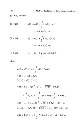
![6.10. Semilinear hyperbolic equations 487
+ /
0
Under the initial premises the functions uo(t) and po(t) are continuous on
the segment [0, T] and the operator kernels K1 (t, s), L1 (t, s), I<~ (t, s)
n2(t, s) are strongly continuous in A(T). Relations (6.10.23)-(6.10.24)
be treated as a system of the Volterra linear equations of the second kind for
the functions u and p. Under such an approach the existence of a solution
to (6.10.23)-(6.10.24) in the class of continuous functions is established
on the whole segment [0, T] in light of the results of Section 5.1. On the
other hand, for any continuous functions u and p the nonhomogeneous
term 9o(t) arising from (6.10.25) is continuous and the kernel K3(t, s) is
strongly continuous. Therefore, equation (6.10.25) is also solvable in the
class C([0, T]; X). In view of this, another conclusion can be drawn that
relation (6.10.18) occurs for T1 = T, thereby justifying the continuous
differentiability of the function u on the segment [0, T] in agreement with
Theorem 6.10.3 and completing the proof of the theorem.~](https://image.slidesharecdn.com/0824719875inverse-141031173353-conversion-gate01/85/0824719875-inverse-508-320.jpg)

![Chapter 7
Two-Point Inverse Problems for
First Order Equations
7.1 Two-point inverse problems
In this section we deal in a Banach space X with a closed linear operator
A with a dense domain. For the purposes of the present section we have
occasion to use two mappings ~: [0, T] ~-~ £(X) and F: [O, T] ~-~ X and
fix two arbitrary elements u0, ul ~ X. The" two-point inverse problem
consists of finding a function u ~ C: ( [0, T]; X ) and an element p E X from
the set of relations
(7.1.i) u’(t) = A u(t) + f(t) , 0 <
(7.1.2) u(0) = u0,
(7.1.3) f(t) = ~(t)p+ F(t), 0 <
(7.1.4) u(T) = ul.
One assumes, in addition, that the operator A is the generator of a strongly
continuous semigroup V(t) or, what amounts to the same things, the
489](https://image.slidesharecdn.com/0824719875inverse-141031173353-conversion-gate01/85/0824719875-inverse-510-320.jpg)
![490 7. Two-Point Inverse Problems for First Order Equations
Cauchy (direct) problem (7.1.1)-(7.1.2)is uniformly well-posed. It is
from Fattorini (1983) that for u0 ¯ 79(A)
f ¯ c1 ([o, T];X )+ C([0T, ];9 (A))
the direct problem (7.1.1)-(7.1.2) has a solution in the class of functions
u ¯ C1([0, T]; X), Au ¯ C([0, T]; X).
This solution is unique in the indicated class of functions and is repre-sentable
by
(7.1.5)
t
u(t) = V(t)uo + / V(t - s) f(s)
0
In contrast to the direct problem the inverse problem (7.1.1)-(7.1.4)
volves the function f as the unknown of the prescribed structure (7.1.3),
where the element p ¯ X is unknown and the mappings q~ and F are
available. Additional information about the function u in the form of the
final overdetermination (7.1.4) provides a possibility of determining the
element p.
In the further development one more restriction is imposed on the
operator-valued function O:
(7.1.6) ¯ ¯ c1 ([0, T]; ~(X)),
which ensures that for any p ¯ X the function O(t)p as a function of
the argument t with values in the Banach space X will be continuously
differentiable on the segment [0, T]. Because of this, the function f of the
structure (7.1.3) belongs to the space
c1([0,T ];X )+ C([0,T ];V (A))
if and only if the function F belongs to the same space. We note in pass-ing
that from relation (5.7.4) and the very definition of the inverse problem
solution it follows that the inclusion ul ¯/)(A) re~gards as a necessary solv-ability
condition. Before proceeding to careful analysis, it will be sensible
to introduce the concept of admissible input data.
Definition 7.1.1 The elements Uo and ul and the function F are called
the admissible input data of the inverse problem (7.1.1)-(7.1.4) if
(7.1.7) Uo, ul ¯ :D(A), F 1( [0, T]; X) + C([ 0, T]; ~D (A))](https://image.slidesharecdn.com/0824719875inverse-141031173353-conversion-gate01/85/0824719875-inverse-511-320.jpg)
![7.1. Two-point inverse problems 491
In the case when the input data are admissible, a solution of the
Cauchy problem (7.1.1)-(7.1.2) can be expressed by (7,1.5), thus causing
the equivalence between the system joining three relations (7.1.1)-(7.1.3)
and the following equation:
t
(7.1.8) u(t) = V(t) uo + j V(t [q)(s ) p + F (s ds,
o
0<t<T.
All this enables us to extract a single equation for the unknown element p.
In view of (7.1.8), relation (7.1.4) becomes
T
ul = v(T) Uo + / V(T- [O(s) p + F(s) ds
o
and admits an alternative form
(7.1.9) Bp = g,
where
(7.1.10)
T
Bp =f y(T- s)e(s)p
0
(7.1.11)
T
g =u, - V(T) Uo - / V(T- s) F(s)
o
This provides sufficient background to deduce that the function u and the
element p give a solution of the inverse problem (7.1.1)-(7.1.4) with admis-sible
input data if and only ifp solves equation (7.1.9) and u is given
formula (7.1.8). Thus, the inverse problem of interest amounts to equation
(7.1.9).
The next step is to reveal some elementary properties of equation
(7.1.9) in showing that its right-hand side g defined by formula (7.1.11)
an element of the manifold 7)(A). Indeed, recalling that u0, ul E 7)(A)
we may attempt the sought function F in the form F = F1 + F2 with
F1 E Cl([0, T]; X) and F2, AF2 ~ C([0, T]; X). From semigroup theory
(see Fattorini (1983)) it is known that the function u defined by (7.1.8)](https://image.slidesharecdn.com/0824719875inverse-141031173353-conversion-gate01/85/0824719875-inverse-512-320.jpg)
![492 7. Two-Point Inverse Problems for First Order Equations
subject to the following relations:
(7.1.12) u’(t) = V(t) (AUo ÷
+~ (o)~ )+ F~’(~)
t
+ / v(~ - s/
0
+ AF~(~)¢+’( ~)p]
(7.1.13) A u(t) = V(t) ( A uo +
+ v(0)p-) F~(,)- ¢(,)
t
+ / v(~- ~)[ r:(~)
0
+ Ar ~(~)+ ~’(~)p]
At the same time, for the element g defined by (7.1.11), the following
relationship takes place:
(7.1.14) Ag =Au~-V(T)(Auo+F~(O))+F~(T)
T
[ V(T-~ ) [ r:(~) + A~ (~)]
0
whence the inclusion g ~ ~(A) becomes obvious. On the other hand, for
uo = 0 and F = 0 we thus have g = u~. Since u~ is ~rbitr~rily chosen from
the manifold ~(A), any element of ~(A) may appear in place of g. Thus,
we arrive at the following assertion.
Corollary 7.1.1 The unique solvability of ~he inverse.problem (7.1.1)-
(7.1.4) wi¢h any admissible inpu~ da~a is equivalen¢ ~o the invertibility of
~ o~o~ ~ ~d ~ ~ ~(~-~) = ~(~).](https://image.slidesharecdn.com/0824719875inverse-141031173353-conversion-gate01/85/0824719875-inverse-513-320.jpg)
![7.1. Two-point inverse problems 493
The operator B-1 (if it ~xists) is closed. This is due to the fact that
the operator B is bounded. It is not difficult to establish this property
with the aid of (7.1.10). If the operator A is unbounded, thus causing that
the manifold D(A) does not coincide with the space X, then the operator
B-1 fails to be bounded. However, the Banach theorem on closed operator
yields
B-1 e £(1)(A),
if the space T)(A) is equipped with the graph norm of the operator
Corollary 7.1.2 If a solution of the inverse problem (7.1.1)-(7.1.4) exists
and is unique for any admissible input data Uo, ul ¯ 7~( A ) and
f =F,+f2
with rl ¯ C’ ([0, T]; X ), F2 ¯ C([O, T]; 79(A)), then the stability estimates
hold:
(7.1.15)I lullc,<[0,al;x)~ c (llu01l~<AI)I÷~ lll~<A)
(7.1.16)
(7.1.17)
÷I I F,I Ic’([O,TII;IXF)2 I I¢([0,T]; v)()a),
IIPI I <c (ll ~oI Iv(a÷) I I ’~,I Iv(~)
Proof Indeed, since the inverse problem of interest is uniquely solvable
under any admissible input data, the operator B is invertible and so
B-1 ¯ £(D(A),
In view of this, a solution to equation (7.1.9) satisfies the inequality
tIP[I-< M ttgII~tA)
whereM - - II B-1I¯I Withth is relatione stablishede, stimate( 7.1.17)imme-diately
follows from (7.1.11) and (7.1.14). When (7.f.8), (7.1.12)-(7.i.13)
and (7.1.17) are put together, we come to (7.1.15) (7.1.16) as d esi red.](https://image.slidesharecdn.com/0824719875inverse-141031173353-conversion-gate01/85/0824719875-inverse-514-320.jpg)
![494 7. Two-Point Inverse Problems fo~" First Order Equations
It is worth noting here that in the genergl case the operator B fails to
be invertible, thus causing some difficulties. This obstacle can be illustrated
by the example in which the operator A has an eigenvector e with associated
eigenvalue A. One assumes, in addition, that ¢(t) is a scMar-vMuedfu nction
such that
T
exp
o
ds:O.
Let the value q%(t) of the function ~ at the point t 6 [0, T] be identified with
the operator of multiplication by the number O(t) in the space X. Turning
now to the inverse problem (7.1.1)-(7.1.4) observe that the function u
the element p are given by the formulae
This pair constitutes what is called a nontrivial solution of the inverse
problem with zero input data u0, ul, F = 0, thereby clarifying that the
operator B transforms the nonzero element e into zero in the space X.
In this connection the conditions, under which the operator B is in-vertible
and equation (7.1.9) is solvable in every particular case, become im-portant
and rather urgent. What is more, we need to know at what extent
a solution to equation (7.1.9) may be nonunique and find out the conditions
under which Fredholm’s solvability of the inverse problem (7.1.1)-(7.1.4)
arises. To overcome difficulties involved in a study of equation (7.1.9) and
stipulated by the fact that this equation is of the first kind, it is reasonable
to reduce it to an equation of the second kind by imposing extra restrictions
on the input data.
Lemma r.1.1 Let ¯ e c1 ([0, T]; £(X)), the operator Op(T) be invertible
and O~(T)-1 6 £(X). If the elemen* g defined by (7.1.11) belongs to the
manifolVd( A)a nde p(A),t he e a (7.1.9) is eV ilent to th
following one:
(7.1.18) p- B~ p = h,](https://image.slidesharecdn.com/0824719875inverse-141031173353-conversion-gate01/85/0824719875-inverse-515-320.jpg)
![7.1. Two-point inverse problems 495
w~e~e
(7.1.19) ~, : ~(T)-i[/ V(T- s)
0
× [¢’(-s ¢)( s)]
+ V(T) ~(0)]]
(7.1.20) h = -q}(T)-i(- A I ) g.
Proof One well-known fact from semigroup theory may be useful in the
further development: for any function f 6 C~ ([0, T]; X)
t t
(7.1.21A) f(O) f(t)
0 0
Since A 6 p(A) and g ~/)(A), equation (7.1.9) is equivalent to the following
one~
(7.1.22) (A-AI)Bp: (A-II)g,
which, in turn, ’can be rewritten as
T
(7.1.23) V(T-s)¢’(s)pds+V(T)¢(O)p-~(T)p
0
T
-~ / V(T-s)~(s)pds : (A-AI)
0
Here we have taken into account (7.1.10) and formula (7.1.21) with f(t)
O(t) p incorporated. Collecting two integral terms in (7.1.23) and applying
then the operator ~(T)-1 to both sides of the resulting equality, we derive
(7.1.18), thereby completing the proof of Lemma7 .1.1.1
In light of the well-known results from semigroup theory there exist
constants M >_ 1 and/9 such that the estimate
(7.1.24) II V(t)ll < M exp(flt)
is valid for any t k 0. This provides suppo.rt for the view that V(t) is a
contraction semigroup if M = 1 and/9 < 0. For a wide range of applica-tions
the corresponding semigroups turn out to be contractive. Moreover,
in some practical problems the constant /9 arising from (7.1.24) is strictly
negative and in every such case the semigroup is said to be exponentially
decreasing.](https://image.slidesharecdn.com/0824719875inverse-141031173353-conversion-gate01/85/0824719875-inverse-516-320.jpg)
![496 7. Two-Point Inverse Problems for First Order Equations
Theorem 7.1.1 If under the conditions of Lemma 7.1.1 estimate (7.1.24)
holds and
T
(7.1.~) / [~’(s) - ~(s)] ~(T)-’ e~p( ~ (T-o
1
+ (I)(O)~(T) -1 exp (/~ T) <
then the operator B is invertible,
7)(B -1) =
and, in particular, the inverse problem (7.1.1)-(7.1.4) is uniquely solvable
for any admissible input data.
Proof By virtue of Lemma 7.1.1 equatio~ (7.1.9) can be replaced
(7.1.18) with
v’ = ¢(T)
Multiplying the resulting equMity by ~(T) from the left yields the governing
equation for the element p’:
(7.1.26) p’ - B~ p’ = h’,
where the expressions
T
B~ = /V(T-s)[~’(s)- ~(s)] ~(T) -1 -d1s , + V(T)~(0)~(T)
0
~’=-(~-~)~
are derived from representations (7.1.19)-(7.1.20). Putting these together
with (7.1.24)-(7.1.25) we conclude that the operator B: has the bound
whence the unique solvability of (7.1.26) follows for any right-hand side
h~ ~ X. Therefore, equation (7.1.18) is also uniquely solvable for any
right-hand side, since the elements h and h~ are related by
h’= e(T)
where ~(T), ~(T) -1 e C(X). For the same reason as before, Lemma
7.1.1 asserts the unique solvability of (7.1.9) for any admissible input data.
Furthermore, on account of Corollary 7.1.1 the operator B is invertible, so
that
V(~-~) = ~(~),
thereby completing the proof of the theorem. ¯](https://image.slidesharecdn.com/0824719875inverse-141031173353-conversion-gate01/85/0824719875-inverse-517-320.jpg)
![7.1. Two-point inverse problems 497
Theorem 7.1.1 applies equally well to one particular problem in which
a scalar-valued function ¯ is defined and continuously differentiable on the
segment [0, T]. We identify the number (I)(t) and the operator of multi-plication
by this number (I)(t) in the space X bearing in mind the inverse
problem (7.1.1)-(7.1.4).
and ¯ as an operator function belongs to the space C1([0, T]; £(X)).
operator ~(T) is invertible if and only if ~(T) # 0 and its inverse coincides
with the operator of multiplication by the number
(1)(T)-:~ ]/4)(T).
Also, for all values t 6 [0, T] we accept
(7.1.27) qb(t) > O’(t) >_
Theorem 7.1.2 One assumes Ihat ~he semigroui3 V(t) generated by the
operalor A obeys estimate (7.1.24) wilh M = 1 and ~9 < O. If Ihe fundion
¯ 6 CI[0, T] is in line with (7.1.27), then a solution of Ihe inverse problem
(7.1.1)-(7.1.4) ezisIs and is unique for any admissible inpuI daIa.
Proof From estimate (7.1.24) it follows that II V(T)II < 1, giving 1 e
p(V(T)). The theorem on mapping of the semigroup spectrum yields the
inclusion 0 ~ p(A), making it possible to apply Theorem 7.1.1 to ,~ = 0.
Denote by Q the left-hand side of inequality (7.1.25). Then
T
Q = l,(r-)*]l l ¢’(,e)xp1(f l (T-s))d s+ I~(O)/4p(T)eIx p(/9T ).
0
Since fl < 0, we obtain for any s 6 [0, T] the quantity
e~p(~(T-s))
and the following chain of relations as an immediate implication of condi-tions
(7.1.27):
T Q < 4~(T)-~ 4f)’(s)d s + ~(T) exp (/9 T)
0
= 42(T-)~ ((I)(T)(-I )(0)+) ~--~
(I)(T() 1 - exp(/ 5 T)).](https://image.slidesharecdn.com/0824719875inverse-141031173353-conversion-gate01/85/0824719875-inverse-518-320.jpg)
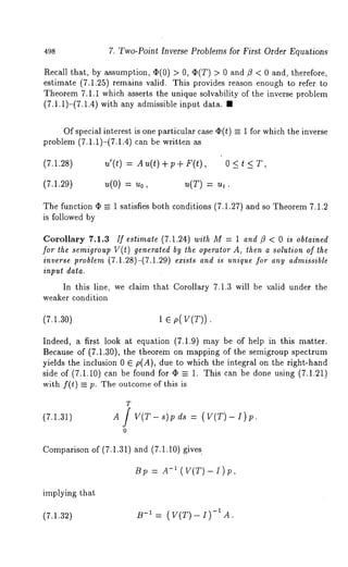
![7.1. Two-point inverse problems 499
With this relation in view, the element p can explicitly be expressed by
(7.1.33) p (V(T) I)-IA
Being concerned with the element f, we find the function u by formula
(7.1.8):
t
(7.1.34) u(t) = V(t)uo+/ V(t-s)[p+F(s)].ds, 0<t<T,
0
since 4~ = 1. Thus, we arrive at the following assertion.
Corollary 7.1.4 ff the semigroup V(t) generated by the operator A sat-isfies
condition (7.1.30), then a solution of the inverse problem (7.1.28)-
(7.1.29) exists and is unique for any admissible input data. Moreover, this
solution is explicitly found by formulae (7.1.11), (7.1.33) and (7.1.34).
In trying to verify condition (7.1.30) some difficulties do arise. How-ever,
for a wide class of problems the theorem on the spectrum mapping is
much applicable and, by virtue of its strong version, we thus have
exp (ta(A)) = ~r(V(t)) {0}.
For example, the problem with a self-adjoint operator A falls into the"
category of such problems and so condition (7.1.30) can be replaced
A-I ¯ £(X). Furthermore, the class we have mentioned above contains
also problems with parabolic equations, since the operator A generates an
analytic semigroup. In this case the meaning of condition (7.1.30) is that
the spectrum of the operator A contains no points of the type 2zrki/T,
where k is an integer and i is the imaginary unit.
As stated above, the inverse problem under consideration may have,
in general, a nontrivial solution even if all of the input data functions
become nonzero. If this inverse problem possesses a compact semigrou’p,
then Fredholm-type solvability of this problem can be achieved. Recall
that the semigroup V is said to be compact if the operator V(t) is compact
for allt >0.
Theorem 7.1.3 If the operator A generates a compact semigroup,
(I) ¯ cl([o, T]; ~(X)) , -1 ¯ ~(X) , )l ¯ p (A)
and the element h is defined by (7.1.20), then the following assertions are
valid:](https://image.slidesharecdn.com/0824719875inverse-141031173353-conversion-gate01/85/0824719875-inverse-520-320.jpg)
![5oo 7. Two-Point Inverse Problems for First Order Equations
(1) for the inverse problem (7.1.1)-(7.1.4) be solvable for any admis-sible
input data it is necessary and sufficient tha~ ~his problem has
only a trivial solution under the zero input data;
(2) the set of all solutions of the inverse problem (7.1.1)-(7.1.4) with
zeroi npudt ataf ormisn thes paceC 1([0,
dimensional subspace;
(3) there exist elements I1, 12,... ,ln C X* such that the inverse prob-lem
(7.1.1)-(7.1.4) is solvable if and only if li(h) = O, 1 < i <
Proof It is clear that all the conditions of Lemm7a .1.1 hold true, by means
of which the inverse problem concerned reduces to equation (7.1.18). Recall
that the semigroup V is compact. Due to this property V will be continuous
for t > 0 in the operator topology of the space £(X). Since the set of all
compact operators constitutes a closed two-sided ideal in this topology, the
operator
(7.1.35) B’ = f V(T- - cts
0
is compact for any s > 0 as a limit of the corresponding Riemann sums in
the space £(X). On the other hand, the norm of the function
f(s) : V(T- s) [¢’(s)
is bounded on the segment [0, T]. Consequently, the integral in (7.1.35)
converges as e -~ 0 in the operator topology of the space £(X), implying
that the operator
T
0
is compact. It should be noted that in Lemma7 .1.1 this integral is under-stood
in the sense of the strong topology of the space £(X).
If the operator V(T) is supposed to be compact, then so is the operator
B" = V(T) ~(0).
For the same reason as before the ~ompactness of the operators B~ and B"
both implies this property for the operator
BI = O(T)-~( ’ +B") .](https://image.slidesharecdn.com/0824719875inverse-141031173353-conversion-gate01/85/0824719875-inverse-521-320.jpg)
![7.1. Two-point inverse problems 5Ol
This serves as a basis for special investigations of equation (7.1.18) from
the viewpoint of Fredholm’s theory.
It is easily seen that the element g defined by (7.1.11) runs over the
entire manifold 7)(A) if the input data run over the set of all admissible
elements. Formula (7.1.20) implies that the element h runs over the entire
space X, while the element g lies within the manifold 7)(A). From such
reasoning it seems clear that the solvability of the inverse problem (7.1.1)-
(7.1.4) under any admissible data is equivalent to that of equation (7.1.18)
for any h E X. Therefore, the first assertion of the theorem is an immediate
implication of Fredholm’s alternative.
If all of the input data become zero, then h = 0, so that the set
comprising all of the solutions to equation (7.1.18) will coincide with the
characteristic subspace of the operator B1 if this subspace is associated with
the unit eigenvalue. Since the operator B~ is compact, the characteristic
subspace so constructed is finite-dimensional. In order to arrive at the
second assertion of the theorem it remains to take into account that (7.1.8)
admits now the form
t
u(t) = / V(t - s) ~(s)p
0
Let {li} form a basis of the finite-dimensional space comprising all of
the solutions to the homogeneous equation l - B~l = 0. From Fredholm’s
theory it follows that equation (7.1.18) will be solvable if and only if l~(h)
0, 1 < i < n. This proves the third assertion, thereby completing the proof
of the theorem. ¯
7.2 Inverse problems with self-adjoint operator
and scalar function
This section is connected with one possible statement of the two-point
inverse problem, special investigations of which lead to a final decision-making
about the existence and uniqueness of its solution. One assumes
that X is a Hilbert space, an operator A is self-adjoint and the inclusion
(I) E C1[0, T] holds. The main goal of our study is to find a function](https://image.slidesharecdn.com/0824719875inverse-141031173353-conversion-gate01/85/0824719875-inverse-522-320.jpg)
![502 7. Two-Point Inverse Problems for First Order Equations
u ¯ C1 ([0, T]; X ) and an element p ¯ X from the set of relations
(7.2.1) u’(t) = Au(t) + f(t), 0 <
(7.2.2) u(O)
(7.2.3) f(t) = (~(t)p+ F(t), 0 < t <
(7.2.4) u(T)
when the function F ¯ C1([0, T]; X) + C([0, T]; D(A)) and the elements
Uo, ul ¯ D(A) are available, that is, the input data comprising F, u0 and
u2 are supposed to be admissible in the sense of Definition 7.1.1.
The operator A is the generator of a strongly continuous semigroup
if and only if it is semibounded from above. In that case there is a real
number b such that the operator A is representable by
b
A = / ~ dE~,
where E~ refers to the spectral resolution of unity of the operator A
(see Akhiezer and Glasman (1966)). Every element h ¯ X can be put
correspondence with the measure on the real line
) = d(E h, h),
where (f, 9) denotes the inner product of elements f and g in the space
A key role in "milestones" with regard to problem (7.2.1)-(7.2.4)
played by the following lemma.
Lemma 7.2.1 Let the operator A be self-adjoint in the Hilbert space X
and E~ be ils spectral resolution of unity. One assumes, in addition, that
the function ~ belongs to the space C(R) and the set of all its zeroes either
is empty or contains isolated points only. Then the equation
is solvable with respect to p if and only if
(7.2.6)
Moreover, equation (7.2.5) with h = 0 has a unique trivial solution if and
only if the point spectrum of the operator A contains no zeroes of the func-tion](https://image.slidesharecdn.com/0824719875inverse-141031173353-conversion-gate01/85/0824719875-inverse-523-320.jpg)
![7.2. Inverse problems with self-adjoint operator 503
Proof The uniqueness of a solution to equation (7.2.5) is of our initial
concern. We proceed as usual. This amounts to considering one of the
zeroes of the function 9, say ,~0, setting h = 0 and adopting ~0 and f as an
eigenvalue of the operator A and the associated eigenvector, respectively.
In accordance with what has been said,
dE),f = ~(~-~o)
where ~(A) stands for Dirac’s measure. Therefore,
= = o
and equation (7.2.5) has a nontrivial solution p =
Arguing in reverse direction we assume that the point spectrum of
the operator A contains no zeroes of the function ~ and
Then
(7.2.7) Ilhll== / ]~(1)l 2 d(E),p,p) =
Since each zero of the function ~ is isolated, relation (,7.2.7) implies that
the function
:
may exercise jumps only at zeroes of the function 9. Let now p ¢ 0. It
follows from the equality
that one of the zeroes of the function 9, say ,~0, should coincide with a
point at which the measure #p(A) has a jump. Consequently, ,~0 of such
a kind would be a jump point of the resolution E),, implying that ,k0 falls
into the collection of the eigenvalues of the operator A. The contradiction
obtained shows that p = 0.1](https://image.slidesharecdn.com/0824719875inverse-141031173353-conversion-gate01/85/0824719875-inverse-524-320.jpg)
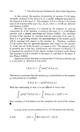
![7.2. Inverse problems with self-ad3oint operator 505
Theorem 7.2.1 If the operator A is self-adjoint and semibounded from
above in the Hilberl space X, #2 E C1[0, T] and ~ ~ O, then the following
asserlions are true:
(1) the inverse problem (7.2.1)-(7.2.4) under the fixed input data is
solvable if and only if
(7.2.9) f l~(~)l-~d(E~g,
where Ez refers to the resolution of unily of the operator A, the
function ~ is specified by (7.2.8), the element 9 is given by relation
(7.1.11), that is,
T
g = u, - V(T~) o- f V(T- s) F(s)
o
and V is a semigroup generated by the operator A;
(2) if the inverse problem (7.2.1)-(7.2.4) is solvable, lhen its solulion
will be unique if and only if the point spectrum of the operator A
contains no zeroes of the function ~ specified by (7.2.8).
Proof The inverse problem (7.2.1)-(7.2.4) is a particular case of the
point problem (7.1.1)-(7.1.4) and, as stated in Section 7.1, can be reduced
to equation (7.1.9) of the form Bp = g, where
T
(7.2.1o) Bp = f v(T- ~)~(~)p
o
Here V refers, as usual, to the semigroup generated by the operator A.
Since the function u is explicitly expressed via the element p by for-mula
(7.1.8), the existence or uniqueness of a solution of the inverse problem
concerned is equivalent to the same properties for the equation Bp = g,
respectively.
As we have mentioned above, there is a real number b such that
b
A = / A dEa.](https://image.slidesharecdn.com/0824719875inverse-141031173353-conversion-gate01/85/0824719875-inverse-526-320.jpg)
![506 7. Two-Point Inverse Problems for First Order Equations
On the other hand, from calculus of self-adjoint operators it is known that
v(t)
b / exp(It) dE),,
which is substitu.ted into (7.2.10) and leads to the formula
T b
It is worth noting here that the measure dE~ ® ds is bounded on (-¢c, b]
[0, T] and the function
K(A,s) = O(s) exp (A (T-is
continuous and bounded on (-~, b] x [0, T]. Due to the indicated prop-erties
the Fubini theorem suits us perfectly for the integrals in (7.2.11) and
allows one to change the order of integration. By minor manipulations with
these integrals we arrive at
b
B = f dE ,
where the function ~ is specified by (7.2.8). What is more, it follows from
(7.2.8) that ~ is an entire function which does not identically equal zero.
In this case the zero set of the function ~ contains isolated points only. To
complete the proof of the theorem, it remains to take into account that
the equation Bp = g is of the form (7.2.5) and apply then Lemma 7.2.1,
thereby justifying both assertions..
Suppose that the zero set of the function ~ does not intersect the
spectrum of the operator A. Under this premise item (2) of Theorem 7.2.1
is certainly true and condition (7.2.9) is still valid for (I)(T) :~ 0. A
observation may be of help in verifying the fact that the integral in (7.2.9)
can be taken from - ~ to a finite upper bound. Also, the integral
(7.2.12)
b f -: d(E g, g)
a](https://image.slidesharecdn.com/0824719875inverse-141031173353-conversion-gate01/85/0824719875-inverse-527-320.jpg)
![7.2. Inverse problems with self-adjoint operator 507
is always finite for any finite numbers a and b, since the function ~ is
continuous, its zero set consists of the isolated points only and the spectrum
of the operatgr A is closed. Indeed, if ~(,~0) = 0, then the resolvent set p(A)
contains not only this point ,~0, but also its certain neighborhood in which
Ea = const. In this view, it is reasonable to take the integral in (7.2.12)
over the segment [a, b] except for certain neighborhoods of all points from
the zero set of the function ~. Therefore, the integral in (7.2.12) is finite
and it remains to establish the convergence of the integral in (7.2.9) at -o~.
To that end, we integrate by parts in (7.2.8) and establish the relation
¯ (0) exp AT- ~(T) 1
(7.2.13) ~o(I)
,~
+ ~
T
x i ¢~’(s) exp(A(T-s))
o
implying that
... ¢(T) /
as ,~ --* -o~. Therefore, the integral in (7.2.9) converges at -ee if and only
if there exists a real number a, ensuring the convergence of the integral
which is just finite due to the inclusion g E O(A) (see Riesz and Sz.-Nagy
(1972)). Recall that the element g was defined by (7.1.11) and its belonging
to the manifold T)(A) was justified at the very beginning of Section 7.1.
From the theory of operators it is known that the spectrum of any self-adjoint
operator is located on the real axis. Hence the function ~o becomes
non-zero on the operator spectrum, provided that none of the real numbers
is included in the zero set of this function. Furthermore, it is supposed that
the function (I) is nonnegative on the segment [0, T] and does not identically
equal zero. On the basis of definition (7.2.8) the condition imposed above
sufficient for the function ~ to become non-zero on the operator spectrum.
Summarizing, we deduce the following corollary.
Corollary 7.2.1 Let the operator A be self-adjoint and semibounded from
above in the Hilbert space X. If the function q~ E C1[0, T] is nonnegative
ande (T)> O,t hena sotutionof the inversper oble(m7. 2.1)-(7.2.4e)x i
and is unique for any admissible input data.](https://image.slidesharecdn.com/0824719875inverse-141031173353-conversion-gate01/85/0824719875-inverse-528-320.jpg)
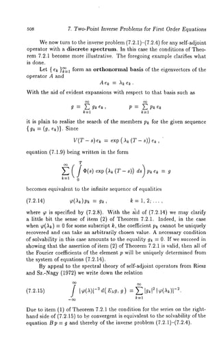
![51o 7. Two-Point Inverse Problems for ~irst Order Equations
Lemma7 .2.1 suits us perfectly in investigating the equation B p = g via
representation (7.2.17) and leads to the following proposition.
Corollary 7.2.2 Let X be a complex Hilbert space and A = i A1, where
AI is a self-adjoint operator in the space X. If, in addition, ¯ E C1[0, T]
and ~ ~ O, then the following assertions are true:
(1) the inverse problem (7.2.1)-(7.2.4) is solvable for the fixed admis-sible
input data Uo, ua and F if and only if
(7.z19) / d(E g, g)
where Ex is the resolution of unity of the operator A1, the function
~1 is defined by (7.2.18), the element g is representable by (7.1.11)
as follows."
T
g : "a 1 V(T) 0 - V( T - 8) F(s ) d8
o
(here V is the group generated by the operator A);
(2) if the inverse problem (7.2.1)-(7.2.4) is solvable, then for its solution
to be unique it is necessary and sufficient that the point spectrum
of the operator A contains no zeroes of the function ~ defined by
(7.2.8).
The second item of the above proposition needs certain clarification.
It is worth bearing in mind some circu-mstances involved. Being multiplied
by i, the point spectrum of the operator A1 turns into the point spectrum
of the operator A. At the same time, t.he zeroes of the function ~a "move"
to the zeroes of the function ~.
Several conditions quoted below assure us of the validi.ty of items (1)-
(2) of Corollary 7.2.2. Recall that the spectrum of the opera.tot A is located
on the imaginary axis. Now the statement of item (3) will be proved if
succeed in showing that the function ¢p has no zeroes on the imaginary
axis or, what amounts to the same, the function ~1 has no zeroes on the
real axis. If, in addition, the inequality I~(0)1 < IO(T)I holds true,
condition (7.2.19) is also true. Indeed, if the function ~ga does not vanish](https://image.slidesharecdn.com/0824719875inverse-141031173353-conversion-gate01/85/0824719875-inverse-531-320.jpg)
![7.2. Inverse problems with self-adjoint operator 511
on the real axis, then it is not equal to zero on the spectrum of the operator
A1 and, therefore, for any D > 0 the integral
DJI~,(~)1-2d (E~g,
-D
is finite.
On the other hand, by integrating (7.2.18) by parts we obtain
(7.2.20) ~1(I) qS(0) ex p(iIT) - 69(T)
iA
1 J TO’(s) exp (iA (T- s))
+~
o
After replacing s by T - s the integral term in (7.2.20) becomes
T
1 /g),l(s) exp(iAs) ds,
iA
o
where ~,(s) = ~(T - s). Whence, by the Riemann lemm~t it follows
T
/ (1)
1
(7.2.21) ~-~ q~’(s) exp (iA (T- s)) =ds , A -~ oc .
o
In conformity with (7.2.21) and the inequality [~(0)] < [q~(T)[, relation
(7.2.20) implies as A ~ cx~ that
so that for all sufficiently large numbers D
I,XI>D I,XI>D
< ~-~ f ; d(E~, g).](https://image.slidesharecdn.com/0824719875inverse-141031173353-conversion-gate01/85/0824719875-inverse-532-320.jpg)
![7. Two-Point Inverse Problems for First Order Equations
Since g 6 Z)(A), the latter integral is finite. The same continues to hold
for the integral in (7.2.19).
At the next stage we state that if the function (I) is nonnegative and
strictly increasing on the segment [0, T] (the inequality lq)(0)l
is due to this fact), then the function ~ defined by (7.2.18) has no
roes on the real axis. Being nonnegative and strictly decreasing on the
segment [0, T], the function q)l(t) = (I)(T - t) is subject to the following
relationships:
Re ~i (,~) = cos (A (T- s))
T
: / (I)(T- s) As d s
T
= ] ~l(s) cos ,ks ds,
0
T ]~(s) sin (A (T- ds
o
T
= J ’~(s) sin )~s
o
Here we used also (7.2.18). Since
T
ae ~, (0) = f ¢1(s) ds
0
and Im~,l(,~) as a function of ,~ is odd, it remains to show that for any
T
(7.2.22) J O1(s) sin as ds >
0
If ,~ > ~r/T, then sin as _> 0 for all s e [0, T] and inequality (7.2.22)
immediately follows. Let ,~ < ~r/T and T # 2~rn/,L Allowing n to be](https://image.slidesharecdn.com/0824719875inverse-141031173353-conversion-gate01/85/0824719875-inverse-533-320.jpg)
![7.2. Inverse problems with self-adjoint operator 513
integer we extend the function ~1 (s) by zero up to the point of the type
27rn/A, which is nearest to T from the right. After that, the integral in
(7.2.22) equals
(7.2.23) E / (I)l(s) sin ds.
k=l 2~(k-1)/a
We claim that every term of the sum in (7.2.23) is positive. Indeed,
~(~k-1)/~
/ opl(s) sin,~sds = J ~(s) sinAsds
2~r(k-1)/A 2~(k-1)/A
q~l (s) sin As ds.
Upon substituting s + ~r/A for A the second integral transforms into the
following ones:
2~r(k-1)/A
(Ih(s) sin As ds = sin as es.
Due to the strict decrease of the function 4p~ on the segment [0, T] it
remains to note that
- + > 0
and sin As > 0 on the segments [2~’(k- 1)/A, ~/(2k- 1)/A]. In accordafice
with what has been said, the following result is obtained.
Zorollary 7.2.3 Let X be a complex Hilbert space and A = iA1, where
A1 is a self-adjoint operator in the space X. If, in. addition, the function
(I) ~ el[0, T] i8 nonnegative and strictly increasing on the segment [0, T],
then a solution of the inverse problem (7.2.1)-(7.2.4) exists and is unique
for any admissible input data.](https://image.slidesharecdn.com/0824719875inverse-141031173353-conversion-gate01/85/0824719875-inverse-534-320.jpg)
![514 7. Two-Point Inverse Problems for First Order Equations
7.3 Two-point inverse problems in Banach lattices
Let X be a Banach lattice, that is, a Banach space equipped with the
partial ordering relation _<; meaning that any pair of its elements f, g E X
has the least upper bound sup (f, g) and the greatest lower bound
inS (f, g). In this case the linear operations artd norm are,consistent with
the partial ordering relation as follows:
(1) f <_ h implies S + h <_ g + h for any h E X;
(2) if f >_ O, then A f >_ 0 for any number A >_ O;
(3) If[ <_ [gl implies [[f[[
We note in passing that item (3) involves the absolute value of the
element f in the sense of the relation
ISl = sup(S,-S).
Before proceeding, it will be sensible to outline some relevant information
which will be needed in the sequel. More a detailed exposition of Banach
lattices is available in Arendt et al. (1986)~ Batty and Robinson (1984),
Birkhoff (1967), Clement et al. (1987), Kantorovich and Akilov (1977),
Krasnoselskii (1962), Schaefer (1974). Any element f e X admits
dan’s decomposition
f
where the elements S+ _> 0 and f- _> 0 are defined to be
S+ = sup (f, 0), S- = sup (-S, 0).
These members are involved in the useful relations
(7.3.1) [f[ = f++f-, inf(f+,f -) =0.
The set X+ consisting of all nonnegative elements of the space X forms a
closed cone of the space X . Any functional from X* is said to be positive
if it takes on nonnegative values on each element of the set X+. For any
element f > 0 there exists a positive functional ~ ~ X* such that p(f) =
thereby justifying that a nonnegative element of the space X equals zero if
and only if all of the positive functionals vanish on this element.
Lemma 7.3.1. Iff e C([a,b]; X+), then
b
(7.3.2) If(t) dt O.
Moreover, if the integral in (7.3.2) becomes zero, then the function f is
identically equal to zero on the. segment [a, hi.](https://image.slidesharecdn.com/0824719875inverse-141031173353-conversion-gate01/85/0824719875-inverse-535-320.jpg)
![7.3. Two-point inverse problems in Banach lattices 515
Proof By assumption, the function f takes nonnegative values only. Hence
the Riemann sums for the integral in (7.3.2) are also nonnegative. Then
so is the integral itself as a limit of such sums, since the cone X+ is closed.
This proves the first assertion of the lemma.
Equating now integral (7.3.2) to zero we assume that there is at least
one point to E [a, b] at which f(to) > 0 and have occasion to use a positive
functional ~ E X* such that
~( f(to))
Since 7~(f(t)) >_ 0 for any t ~ [a, b], the inequality
b
f f(t)) >.o
holds. On the other hand,
The contradiction obtained shows that the above assumption fails to be
true and in this case the function f is identically equal to zero on the
segment [a, hi, thereby completing the proof of the lemma."
In later discussions we shall need the concepts of positive operator
and positive semigroup. An operator U ~ £(X) is said to be positive if
U(X+) C X+. The positiveness of the operator U will be alw.a_ys indicated
by the relation U >_ 0. A semigroup V is said to be positive if the operator
V(t) >_ for an y t _>0. Advanced theory of positive ope rators and positive
semigroups is available in Arendt et al. (1986), Batty and Robinson (1984),
Clement et al. (1987).
We now consider in the Banach lattice X the two-poin.t inverse prob-lem
of finding a function u ~ C1([0, T]; X) and an element p ~ X from
the set of relations
(7.3.3) u’(t)=Au(t)+O(t)p+F(t), 0<t<T,
(7.3.4) u(0) = u0,
(7.3.5) u(T) = u~](https://image.slidesharecdn.com/0824719875inverse-141031173353-conversion-gate01/85/0824719875-inverse-536-320.jpg)
![516 7. Two-Point Inverse Problems for First Order Equations
for all admissible input data
Uo, U, 67)(A), F6CI([O,T];X) +C([O,T];7)(A)).
Theorem 7.3.1 One assumes that the spectrum of the operator A is located
in the half-plane ()~: Re)~ < 0 and th is op erator ge nerates a positive
semigroup. If
(I) e ~ ([0, T], £(X))
and for any t ~ [0, T]
¯ (t) > o, ~’(t) > o,
then a solution u, p of the inverse problem (7.3.3)-(7.3.5
the constraints
¯ (T)-1 e ;(X), ¯ (T) -I _> 0
is unique under
Proof The theorem will be proved if we succeed in showing that the inverse
problem (7.3.3)-(7.3.5) with zero input data u0, ul, F --- 0 can have
trivial solution u = 0, p = 0 only. To that end, the following system
(7.3.6) u’(t) = A u(t) + ~(t)p, 0 < t < T,
(7.3.7) u(o) =
(7.3.8) u(T) :
complements later discussions. In conformity with the results of Section
7.1, relations (7.3.6)-(7.3.8) take place if and only
t
(7.3.9) u(t) = / V(t - s)~(s)p
where V(t) denotes, as usual, the semigroup generated by the operator A
and the element p satisfies the equation
(7.3.10) B~, : 0,
where the operator B acts in accordance with the ~:ule
T
(7.3.11) Bp = / V(T ds.
0](https://image.slidesharecdn.com/0824719875inverse-141031173353-conversion-gate01/85/0824719875-inverse-537-320.jpg)
![7.3. Two-point inverse problems in Banach l~.ttices 517
Via Jordan’s decomposition p = p+-p- of the element p in the Banach
lattice X we are led to the two associated Cauchy problems
f u’+(t) = Au+(t)+~(t)p +, O<t <T,
(7.3.12) u+(0) =
and
u’_(t) Au_(t)+¢(t)p-, 0<t<T,
(7.3.13)
u_(0) =
whose solutions are given by the formulae
t
u+(~) = / y(~ - s)~(s)p+
0
and
t
~_ (t) = ] v(t - s) ~(s) ~,
0
respectively. From the theory of semigroups we know that for any f 6
C1 ([0, T]; X) the function
t
u(t) = / V(t- s)f(s)
0
is continuously differentiable on the segment [0, T] and
t
u’(t) = ] V(t - s) f’(s) ds + V(~)
0
From such reasoning it seems clear that
T
u’+( T) = ] V(T- 8) ~’(s)p +d 8+ ¢(0)p +,
0
.t(T) =
T f V(T - s) ~’(s)p-
0
ds+ V(T~)( 0p)- .](https://image.slidesharecdn.com/0824719875inverse-141031173353-conversion-gate01/85/0824719875-inverse-538-320.jpg)
![52o 7. Two-Point Inverse Problems for First Order Equations
is a continuous function with values in X+. On account of Lemm7a .3.1 this
function is identically equal to zero on the segment [0, T] and, in particular,
0 : f(T) : ~(T)
implying that p+ = 0, because the operator ¢(T) is invertible. Along
similar lines, the equality
T
u_(T) = J V(T- s)~(s)p-
0
in combination with Lemm7a .3.1 assures us of the validity of the equality
p- = 0. Consequently, having stipulated condition (7.3.9), the element
p = p+ - p- and the function u are equal to zero, thereby completing the
proof of the theorem. ¯
Corollary 7.3.1 ff under the conditions of Theorem 7.3.1 the semigroup
generated by the operator A is compact, then a solulion u, p of the inverse
problem (7.3.3)-(7.3.5) exists and is unique for any admissible input data.
Proof To prove this assertion, we first refer to Theorem 7.3.1 and thus
ensure the uniqueness here. On the other hand, by Theorem 7.1.3 of Section
7.1 the solvability of the inverse problem (7.3.3)-(7.3.5) is of Fredholm’s
character, due to which the desired result immediately follows from the
uniqueness property. ¯
In concluding this section we note that if the operator A generates a
strongly continuous semigroup, then its spectrum is located in a half-plane
{ ,~: Re A < w } and by virtue of the conditions of Theorem 7.3.1 some
restrictions on this operator do arise naturally. In trying to overcome the
difficulties involved the substitution u(t) = v(t) ~ helps s et u p t he i nverse
problem (7.3.3)-(7.3.5) as follows:
(7.3.19)
v’(t) = A1 v(t) + ¢~l(t)p+ F~(t),
v(O) = vo,
v(T)
0<t<T,](https://image.slidesharecdn.com/0824719875inverse-141031173353-conversion-gate01/85/0824719875-inverse-541-320.jpg)
![7.3. Two-point inverse problems in Banach lattices 521
where
Ax = A-wI,
,~(~) : ,~(~)~-~,
r,(t) r(t) e -"~t,
By applying the results obtained in Theorem 7.3.1 and Corollar)~ 7.3.1 to
problem (7.3.19) we arrive at the following assertions.
Corollary 7.3.2 Let the spectrum of the operator A lie in a half-plane
{ Re ~ < w } and A be the generator of a positive scmigroup. One’assumes,
in addition, that for any t ¯ [0, T]
¢ ¯ C~ ([0, ~1; ~(X))
~(t) >_ 0 and ~’(t)-w ~2(t) >_ O. If -1 ¯ I:( X)and 42(T)-1 >_ O, then
a solutioun, p of thei nversper oble(7m.3 .3)-(7.3u.5nq)i ue.
Corollary 7.3.3 If under the conditions of Corollary 7.3.2 the semigroup
generated by the operator A is compact, then a solution of the inverse prob-lem
(7.3.3)-(7.3.5) exists and is unique for any admissible input data.](https://image.slidesharecdn.com/0824719875inverse-141031173353-conversion-gate01/85/0824719875-inverse-542-320.jpg)

![Chapter 8
Inverse Problems for
~f Second Order
Equations
8.1 Cauchy problem for semilinear hyperbolic equations
In Banach spaces X and Y we deal with a closed linear operator A with a
dense domain, the elements u0, ul E X and the mappings
F: [O,T]xXxXxY~--~X
and
B: X~Y, ¢: [0, T]~Y.
It is required to recover a pair of the functions
~ e c2([0T, ];x ), p e c([o,T ];~ ),
523](https://image.slidesharecdn.com/0824719875inverse-141031173353-conversion-gate01/85/0824719875-inverse-544-320.jpg)
![8.1. Cauchy problem for semilinear hyperbolic equations 525
and the subspace
(8.1.6) ~7 = {x: C(t)
which becomes a Banach space with the appropriate norm
O<t<l
There exist two constants M > 1 and w > 0 such that the cosine and sine
operator functions satisfy on the real line the appropriate estimates
(8.1.8) )I.lc(t)ll <_ M exp(wt), Ils(t)H <_ Mltlexp(wt
For the operator A to generate a strongly continuous cosine function sat-isfying
estimate (8.1.8) it is necessary and sufficient that any number
with ,~ > w complies with the inclusion 12 ¯ p(A) and the collection of
inequalities
d n
Mn!
~-~ [~R(~2’A)] -< (~_~)~+1 n=0, 1,2,...,
where R()~,A) = ()~I- A)-1 refers to the resolvent of the operator A.
Any self-adjoint operator in a Hilbert space generates a str’ongly continuous
cosine f unction if and only if this operator is semibounded from above.
For any Uo e T)(A), ul ¯ E, F 1([0, T]; X) UC([0, T]; V( A))
solution of the Cauchy problem (8.1.4)-(8.1.5) exists and is unique in
class of functions
~ ¯ c2([o,T ];x ) ~ C~([OT,] ;Z )~ C([OV, (A)
Moreover, this solutions is given by the formula
(8.1.9)
t
~,(t)= c(t) ~o+ s (t) ~,~+ f s(t - s)
0
In real-life situations there is a need for certain reduction of the governing
equation of the second order to a first order equation. One way of proceed-ing
is due to Kisynski (1972) and involves the Banach space A" = E x
and the operator](https://image.slidesharecdn.com/0824719875inverse-141031173353-conversion-gate01/85/0824719875-inverse-546-320.jpg)
![526 8. Inverse Problems for Equations of Second Order
with the domain ~(.A) = /)(A) x E. If the operator A is the generator
of the strongly continuous cosine function C(t) associated with the sine
function S(t), then the operator A will generate in the space X the strongly
continuous group
(8.1.11)
Upon substituting
(8.1.1~)
v(t) : (AcS((~~) Cs)((~~))~]
iT(t) = F(t ’ Wo =
the Cauchy problem (8.1.4)-(8.1.5) amounts to the Cauchy problem asso-ciated
with the equation of the first order
w’(t) = A w(t) + iT(t), 0 < t
(8.1.13)
w(O) w0.
Without loss of generality the operator A is supposed to be invertible.
Indeed, making in equation (8.1.1) the replacement
u(t) = v(t) exp( ~ t)
with any A being still subject to the inclusion A~ E p(A) we set up another
inverse problem for the functions v and p
O<t<T,
v’(0) = vl,
0<t <T,
v"(t) = A~ v(t) + F~(t, v(t), v’(t),
v(O) = vo,
B v(t) = ¢~(t),
where
Fx(t,v, vl,p) = exp(-At)
x F(t, exp(At)v, exp(At)(vl+Av),p)-2Av,,
VO ~ ItO 1 Vl ~ Ul -- A u 0 1
~b~(t) = exp (-,~t) ~fl(t),
Aa = A-I~I.](https://image.slidesharecdn.com/0824719875inverse-141031173353-conversion-gate01/85/0824719875-inverse-547-320.jpg)
![8.1. Cauchy problem for semilinear hyperbolic equations 527
The emerging inverse problem is of the same type as the initial one, but
here the operator A is invertible and generates a strongly continuous cosine
function.
For the given function ¢ ¯ C2([0, T]; Y) and element u0 ¯ ~D(BA)
the element Zo is defined to be
(8.1.14) z0 = ¢"(0) BAuo - BFl(O, uo ,ux),
where F1 is involved in the approved decomposition
(8.1.15) F(t,u,v,p) = F~(t,u,v)+ F2(t,u,v,p).
With these ingredients, we impose the following conditions:
(A) the equation B F2(O, uo,ul,p) = Zo with respect to p has a unique
solution Po ¯ Y;
(B) there exists a mapping
Fa: [O, T] x Y x Y x Y H Y
such that
(8.1.16) B F2(t,u,v,p) = Fa(t, Bu, Bv,p);
(C) there is a number R > 0 such that for any t ¯ [0, T] the mapping
z = Fa(t, ¢(t), ¢’(t), p) as afuncti(~n ofp basin the ballSv(po, R)
the in verse
(8.1.17) p = ~(t,z).
Let the operator B comply with
(8.1.18) B ¯ £(:D(A’~), V),
where m is a nonnegative integer and the manifold ~.(A"~) is equipped
with the graph norm of the operator A"~. Extra smoothness conditions are
required to be valid by relating the operator A to be invertible:
(D) there is number R > 0 such th at on the manifold
So = {(t,u,v,p):O<t <T,](https://image.slidesharecdn.com/0824719875inverse-141031173353-conversion-gate01/85/0824719875-inverse-548-320.jpg)
![528 8. Inverse Problems for Equations of Second Order
the functions F1 and F~ are continuous in t and ~atisfy the Lipschitz
condition with respect to (u, v,p) in the norm of the space X. On
the manifold
the functions
and
IIv- ulllE ~ n, IIp-;o IIy ~ R}
Fl(t, A-lu, V)
F2(t,A -luv, ,p)
are continuous in t and satisfy the Lipschitz condition with respect
to (u, v,p) in the norm of the space E. On the manifold
]1 v - Am ~1 I1~-< ~ , II p- poI 1,,_ <~ }
both functions
and
AmFl(t,A-m-lu,.A-mv)
AmF~(t,A-’~-~u,A-~v)
are continuous in t and satisfy the Lipschitz condition with respect
to (u, ~,p) in the norm of the space E;
(E) there is a value R > 0 such that on the manifold
Sy(zo,R,T) {(t,z): 0<t<T, II Z- zolly < R }
the mapping (8.1.17) is continuous in t and satisfies the Lipschitz
condition in z.
Theorem 8.1.1 Let the operator A generate a strongly continuous cosine
function in the space X, A-1 e £(X) and condition (8.1.18) hold. If
the inclusions uo E :D(Am+I), ul ~ :D(Am) and Am ul ~ E occur, where
the space E is the same as in (8.1.6), and all the conditions (A)-(E)
fulfilled, lhen there ezists a number T~ > 0 such lhat on the segment [0,
a solution u, p of the inverse problem (8.1.1)-(8.1.3) exists and is unique
in the class of functions
~ ~ c~([o, :q]; x), ; e c([o, ~]; Y).](https://image.slidesharecdn.com/0824719875inverse-141031173353-conversion-gate01/85/0824719875-inverse-549-320.jpg)
![53o 8. Inverse Problems for Equations of Second Order
which serve to motivate that
ue c1 ([0, T];V (Am))
and
( "~ u(t))’ = "~u’(t ),
since
g)(A2"~) = 2)(A’~) x 2)(A’~).
From (8.1.18)it follows that for each solutfon of problem (8.1.1)-(8.1.3)
(8.1.23) B ~’(t) = ¢’(t), 0 < t < T.
Commopnr actice involves the operator
and the function ~(t) = ¢’(t), by means of which it is easily verified
condition (8.1.3) is equivalent on the strength of (8.1.23) to the following
one:
(8.1.24) 13w(t) = ~(t), 0 < t < T.
Having stipulated condition (8.1.18), the inclusion
occurs and provides reason enough to reduce the inverse problem (8.1.1)-
(8.1.3)t o the inverse problem (6.5.1)-(6.5.a)w e have posed in Section 6.5
for a first order equation. Under the conditions of Theorem 8.1.1 problein
(8.1.19)-(8.1.20), (8.1.24) satisfies the premises of Theorem 8.5.3 with
in place of m. Thus, the desired assertion is an immediate implication of
Theorem 6.5.3, thereby completing the proof of the theorem.I
Of special interest is the case when the function F invol%d in (8.1.1)
is linear with respect to the variables u, u’ and p, that is,
F(I, tt, ~tt, p) = L1( t) ~ -~-L2( ~) t -~L3( t)p -~
where for each fixed numbers t ¯ [0, T] the operators L~(t) ¯ Z;(E,
L~(t) ¯ £(X), La(t) £( Y,X) and th e va lue F(t) ¯ X.All this enabl es
us to prove the unique solvability of the inverse problem concerned on the
whole segment [0, T].](https://image.slidesharecdn.com/0824719875inverse-141031173353-conversion-gate01/85/0824719875-inverse-551-320.jpg)
![8.1. Cauchy problem for semilinear hyperbolic equations 531
Theorem 8.1.2 Let the operator A generate a strongly continuous co-sine
function in the space X, A-1 ¯ ~(X), condition (8.1.18) hold, Uo ¯
:D(A’~+I), Ul ¯ ~P(A’~) and A"~ ul ¯ E, where the space E is the same as
in (8.1.6). One assumes, in addilion, that ¢ ¯ C2([0, T]; Y ), B Uo = ¢(0)
and Bul = ¢’(0). Let representation (8.1.25) take place with the op-erator
functions L1 ¯ C([0, T]; ~.(E,X)), -~ ¯ C([ 0, T]; £(X, E)),
A"~ L~ A-’~-1 ¯ C([0, T]; E(X, E)),
L~ ¯ C([0, T]; £(X) £(E)), A"~ L~ A-’~ ¯ C([0, T]; £(E))
and
A"~ L3 ¯ C([O, T]; £(Y,X)).
If the function A’~F belongs to the space C([0, T]; E), the operator B L3(t)
is invertible for each t ¯ [0, T] and
(BL3)-’ ¯ C([0, T]; £(Y)),
then a solution u, p of the inverse problem (8.1.1)-(8.1.3). exists and is
unique in the class of functions
u ¯ C2([0, T]; X), p ¯ C([0, T];
Proof Exploiting the fact that the inverse problem (8.1.1)-(8.1.3) can
reduced to problem (8.1.19)-(8.1.20), (8.1.24) we may attempt the function
:P(t, w,p) arising from (8.1.19)in the form
(8.1.26) Jr(t, w,p) = £1(t) w + £~(t)p +
where
/:~(t)p= L~(t)p
0 )
wl + L2(t) w2
(tl (o) ¯
It is straightforward to verify that
.A~I(t).A_I
(L2(t)
)-L1l(t)n
= 0 0 ’
~l(t).A -2m-1 _--
(A’~
L~(i) -~
0
A~+~ £~(t)p ( A~ L~(t)
0 ’
A=m+~ ~(t)=
)-A’’~*- ~LI(t)A
0 ’
B L~(t) = B L3(t)](https://image.slidesharecdn.com/0824719875inverse-141031173353-conversion-gate01/85/0824719875-inverse-552-320.jpg)
![532 8. Inverse Problems for Equations of Secdnd Order
Now, by assumption, problem (8.1.19)-(8.1.20), (8.1.24), (8.1.26) satisfies
all the conditions of Theorem 6.5.4 with replacing m by 2 m and so the
desired assertion is an immediate implication of Theorem 6.5.4. Thus, we
complete the proof of the theorem. ¯
Assume now that the smoothing effect of the operator B is well-characterized
by the inclusions
(8.1.27) B ¯ £(X,Y), BA ¯ £(E,Y).
In such a setting it is sensible to introduce the notion of weak solution
and there is a need for some reduction. With the aid of relations (8.1.12)
problem (8.1.4)-(8.1.5) amounts to problem (8.1.13). In view of this,
function u is called a weak solution of problem (8.1.4)-(8.1.5) if the ft~nc-tion
w gives a continuous solution of the reduced problem (8.1.13).
stated in Section 5.2, a continuous solution of problem (8.1.13) exists and
is unique for any w0 ¯ X and any ~- ¯ C([0, T]; X). Furthermore, this
solution is given by the formula
w(t) = v(t) ~o + / w(t - s) ~:(~)
0
where V(t) refers to the semigroup generated by the operator ,4. As a
matter of fact, V(t) is a group and is representable by (8.1.11), establishing
the appropriate link with the cosine function of the operator A. Coming
back to problem (8.1.4)-(8.1.5) we observe that its weak solution is nothing
more than a function u being continuously differentiable on the segment
[0, T] and solving equation (8.1.4) in a sense of distributions. This solution
exists and is unique for any u0 ¯ E, ul ¯ X and F ¯ C([0, T]; X ), and
given by formula (8.1.9) as follows:
t
u(t) = c(t) uo + s(t) ul + / s(t - ds,
0
t
(8.1.28) u’(t) = AS(t)uo +C(t)u, + / C(t - ds.
0
The concept of weak solution of the inverse problem at hand needs certain
clarification. A pair of the functions
u ¯ CI([O,T]; X), p ¯ C([O, T]; Y)
so that](https://image.slidesharecdn.com/0824719875inverse-141031173353-conversion-gate01/85/0824719875-inverse-553-320.jpg)
![8.1. Cauchy problem for semilinear hyperbolic equations 533
is said to be a weak solution of the inverse problem (8.1.1)-(8.1.3) if
the function
F(t) = r(t, u(t), u’(t),p(t))
the function u gives a weak solution of the direct problem (8.1.4)-(8.1.5)
and relation (8.1.3) is satisfied in a pointwise manner. It is easy to verify
that a pair of the functions u, p gives a weak solution of the inverse problem
(8.1.1)-(8.1.3) if and only if the pair w, p as the outcome of the reduction
procedure (8.1.12) is a continuous solution of the inverse problem (8.1.19)-
(8.1.20), (8.1.24) in the sense of the definition of Section
The next step is to redefine the element z0 involved in condition (A)
by means of the relation
(8.1.29) z0 = ¢"(0) B A Uo- B FI(O, no,
thereby excluding (8.1.15) from further consideration, and replace condi-tion
(D) by the following one:
(D1) there exists a number R > Osuch that on the manifold So the
functions FI and F~ are continuous in t and satisfy the Lipschitz
condition with respect to (u, v, p).
Recall that the manifold S0 was defined earlier in condition (D) of the
present section.
Theorem 8.1.3 Let the operator A generate a strongly continuous cosine
function in the space X, conditions (8.1.27) hold, uo G E, ut E X, ¢ G
C2([0, T]; Y), Bu0 = ¢(0) and Bu~ = ¢’(0). Under conditions (A)-(C),
(D1) and (E) there exists a value TI > 0 such that on the segment [0, T~]
a weak solution u, p of the inverse problem (8.1.1)-(8.1.3) exists and is
unique.
Proof As indicated above, replacement (8.1.12) may be of help in reducing
the question of existence and uniqueness of a weak solution of the inverse
problem (8.1.1)-(8.1.3) to the question of existence and uniqueness
continuous solution of the inverse problem (8.1.19)-(8.1.20), (8.1.24).
condition (8.1.27) it seems clear that the inclusions
hold true, since
As can readily be observed, the conditions of Theorem 6.3.1 are fulfilled
and assure us of the validity of the desired assertion.~](https://image.slidesharecdn.com/0824719875inverse-141031173353-conversion-gate01/85/0824719875-inverse-554-320.jpg)
![534 8. Inverse Problems for Equations of Second Order
Following the same procedure one can establish the conditions under
which the function u solving the inverse problem (8.1.1)-(8.1.3) is twice
continuously differentiable. Before giving further motivations, let us replace
conditions (D1) and (E) by the following ones:
(D2) there exists a number R > 0 such that the functions F1 and F2 as
mappings from So into X are Frechet differentiable and their partial
derivatives in every direction are continuous in t and satisfy the
Lipscbitz condition with respect to (u, v, p) in the operator norm;
(E2) there exists a number R > 0 such that the function defined by
(8.1.17) is Frechet differentiable as a mapping from Sy(zo,R,T)
into Y and its partial derivatives Ot and ~z are continuous in t and
satisfy the Lipschit~ condition with respect to z in the operator
norm.
By simply applying Theorem 6.3.2 to the inverse problem (8.1.19)-
(8.1.20), (8.1.24) we arrive at the following assertion.
Corollary 8.1.1 Let the operator A generate a strongly continuous cosine
function in the space X, conditions (8.1.27) hold, uo ¯ D(A), ul ¯
¢ ¯ Ca(J0, ~; Y), Buo = ¢(0) and Bul = ¢’(0). Under conditions (A)-
(C), (02) and (E2) there exists a value T1 > 0 such that on the segment
[0, T~] a solution u, p of the inverse problem (8.1.1)-(8.1.3) exists and is
unique in the class of functions
u ¯ 02([0, T~]; X) ~ O([O, T~]; D(A)), v ¯ :q]; Y).
We begin by investigating the linear case (8.1.25) and approving for
further development the same framework as we dealt before. To obtain
here the solvability of the inverse problem concerned on the whole seg-ment
[0, T], we apply Theorem 6.4.1 of Section 6.4 to the inverse problem
(8.1.19)-(8.1.20), (8.1.24), (8.1.26), whose use permits us to establish
following proposition.
Corollary 8.1.2 Let the operator A generate a strongly continuous co-sine
function in the space X, conditions (8.1.27) hold, the inclusions
Uo ¯ E, ul ¯ X and ~b ¯ C~([0, T]; Y) occur and the equalities
= ¢(0), ¢’(0)
hold. Let representation (6.1.25) hold with the operator functions
L~ ¯ C([0, T]; ~(E, X)), L2 ¯ Ci[0, T]; C(X))](https://image.slidesharecdn.com/0824719875inverse-141031173353-conversion-gate01/85/0824719875-inverse-555-320.jpg)
![8.1. Cauchy problem for semilinear hyperbolic equations 535
and
L3 ¯ C([0, T]; £(V, X)).
If the function F belongs to the space C([0, T]; X ), the operator B L3(t)
in the space Y is invertible for each t ¯ [0, T] and
(BL~)-I ¯ C([0,
then a weak solution u, p of the inverse problem (8.1.1)-(8.1.3) exists and
is unique on the whole segment [0, T].
One may wonder when a weak solution becomes differentiable. The
answer to this is obtained by applying Theorem 6.4.2 to the inverse problem
(8.1.19)-(8.1.20), (8.1.24), (8.1.26).
Corollary 8.1.3 Let the operator A generate a strongly continuous cosine
function in the space X, condition (8.1.27) hold, the inclusions Uo ¯ ~D(A),
ul ¯ Ea n~¢ ¯ C3([0T, ];Y )o ccuarn ~
B u0 = ¢(0), B ~1 = ¢’(0).
Let representation (8.1.25) take place with the operator functions L1 ¯
C1 ([0, T]; I:(E,X)), L2 C1([0, T] ; ~; (X)) and La. ¯ C1([0 , T]; £(Y,X)).
If the function F belongs to the space C1([0, T]; X ), the operator B L~(t)
in the space Y is invertible for each t E [0, T] and
(BL 3)-1 ¯ C([0, T]; £(V))
then on the segment [0, T] a solution u, p of the inverse problem (8.1.1)-
(8.1.3) exists and is unique in the class of functions
u e C~([0, T]; X) N C1([0, T]; E) N C([0, T]; :D(A)),
; e c1 ([0, T];v ).
In just the same way as we did for the first order equations it is plain
to derive an equation "in variations" for the inverse problem (8.1.1)-
(8.1.3). Rigorous assertions follow from Corollary 6.4.2 and are formulated
below.](https://image.slidesharecdn.com/0824719875inverse-141031173353-conversion-gate01/85/0824719875-inverse-556-320.jpg)
![536 8. Inverse Problems for Equations of Second Order
Corollary 8.1.4 Lel, in addition to the conditions of Corollary 8.1.1,
the functions F1 and F: be twice Frechet differenliable on the manifold So
and the function defined by (8.1.17) be twice Frechet differentiable on the
manifold Sy(Zo,R,T). /f¢ ¯ C4([0, T]; Y), ul ¯ D(A)
Auo+ F(O, uo,ul,po) ¯
then there exists a value 0 < T1 <_ T such that on the segment [0, T1] the
functions
~ ¯ c~([o, T,]; x)
and
v ¯ c2([0, T1]; Y).
Moreover, the functions v -- up and q = pl give a solution of the inverse
problem
(8.1.30)
v"(t) = A v(t) + KI (t)v(t) + K~(t)v’(t) + I(3(t)q(t)
v(0) = vo, v,(0) v~,
B v(t) = g(t),
where
Kl(t) = Fu(t, u(t), u’(t),p(t)),
~;~(t=) r ., (t, u(t),, ~’(t),~ (t)),
Ka(t) = Fp(t, u(t), u’(t),.p(t)),
h(t) = Ft(t, u(t), u’(t),p(t)),
VO "~ Ul,
~)1 -= Auo+ F(O, uo,ua,po),
~(t) = ¢’(t).
Corollary 8.1.5 Let, in addition to the conditions of Corollary 8.1.3,
L, ¯ C2([0, T];£(E,X)),L~ C2([0, T];£.(X)), L3 C~([0, T];£. (Y,X))
and F ¯ C2([0, T]; X), ¢ ¯ C4([0, T]; Y ), ul ¯ 73(A),
A Uo + L~ (0) Uo + L~(0) I --~L~i0) Po +F(0) ¯ E .](https://image.slidesharecdn.com/0824719875inverse-141031173353-conversion-gate01/85/0824719875-inverse-557-320.jpg)
![8.1. Cauchy problem for semilinear hyperbolic equations 537
Then u ¯ C3([0, T]; X),
q = p~ give a solution of the inverse problem (8.1.30) wi~h
h’~(t) = L~(t), K~(t) : L:(t), h’~(t) L3(t),
h(t) = L’~( t)u(t) + L’~(t)u’(t)
Vo = u~, v~ = Auo + L~(O) uo + L~(O)u~ + L3(O)po +
g(t) ¢’(t).
By successively applying Corollaries 6.1.4-6.1.5 it is not difficult to
derive the conditions under which solutions of the corresponding inverse
problems as smooth as we like.
8.2 Two-point inverse problems for equations of hyperbolic type
We consider in a Banach space X the inverse problem for the hyperbolic
equation of the second order
(8.2.1) u"(t) = Au(t)+(b(t)p+. 0<t<T,
(8.2.2) u(0) = ~0, ~’(0)
(8.2.3) u(T) = u~.
Being concerned with the operator A, tt~e operator function ~(t) with
values in the space £(X), the function F with values in the space X and the
elements u0, ua and u~, we are looking for a function u ¯ C~ ([0, T]; X )
C([0, T]; D(A)) and an element p e X.. Equation (8.2.1) is said
hyperbolic if the operator A. generates a, strongly continuous cosine
function. As in Section 8.1 the main attention in the study of the inverse
problem (8.2.1)-(8.2.3) is paid to the question of well-posedness of
direct problem
(8.2.4)
(8.2.5)
u"(t) = Au(t)+f(t), O<t
~(0) = ~o, ~’(0) =
In order to retain the notations of Section 8.1 we will use in this section
the symbol C(t) for the cosine function generated by the operator A and](https://image.slidesharecdn.com/0824719875inverse-141031173353-conversion-gate01/85/0824719875-inverse-558-320.jpg)
![538 8. Inverse Problems for Equations of Second Order
the symbol S(t) for the associated sir)e function. The subspace comprising
all continuously differentiable vectors of the cosine function is denoted by
E. This subspace with the accompanying norm (8.1.7) becomes a Banach
space. If u0 e ~(A), ul e E and f e Cl([0, T]; X) + C([0, T]; 7?(A)),
then a solution of the Cauchy problem (8.2.4)-(8.2.5) exists and is unique
in the class of functions
u e C2([0, T]; X) {"1 C([0, T];/)(A))
(for more detail see Fattorini (1969a,b), Kurepa (1982), Travis and
(1978), Vasiliev et al. (1990)). Eurthermore, this solution is expressed
(5.3.12) of Section 5.3 as follows:
(8.2.6) u(t) = C(t) Uo + S(t) ~, + / S(t - s). ds.
o
Note that (8.2.1) and (8.2.2) coincide with (8.2.4) and (8.2.5), respectively,
in one particular case when
(8.2.7) J’(t) = ~(t) p + F(t).
The inverse problem (8.2.1)-(8.2.3) is ~olvable only under the agree-ment
u~ E D(A). In what follows we keep ¯ E 1 ([0, T ]; X ). In that cas
for any p ~ X, the function f specified by (8.2.7) belongs to the space
C1([0, T]; X) + C([0, T]; ~D(A)) if and only if so does the function
this regard, it will be sensible to introduce the notion of admissible input
data. By the input data of the inverse problem concerned we mean the
elements u0, ul, u~ and the function F.
Definition 8.2.1 The input data of the inverse problem (8.2.1)-(8.2.3) is
said to be admissible if uo, u~ ~ 7)(A), ul ~ E
F e C1 ([0, T]; X ) + C([0, T]; 77(A))
We note in passing that for any admissible input data the inverse
problem (8.2.1)-(8.2.3) reduces to a single equation for the unknownp .
deed, if this element is sought by substituting into (8.2.1), then the function
u is given by formulae (8.2.7)-(8.2.8) as a solution of the direct problem
(8.2.1)-(8.2.2). On the other hand, conditi6n (8.2.3) is equivalent to
tion (8.2.6) for t = T with u2 in place of u(T), that is,
T
(8.2.8) u~ : C(T) Uo + S(T) u, + / S(t - s) [ 42(s) + F(s)] ds,
o](https://image.slidesharecdn.com/0824719875inverse-141031173353-conversion-gate01/85/0824719875-inverse-559-320.jpg)
![8.2. Two-point inverse problems for equations of hyperbolic type 539
where all the terms are known except for the element p. Equation (8.2.8)
can be rewritten as
(8.2.9) B p = g,
where
(8.2.10)
T
B = IS(T- s)¢~(s)
o
(8.2.11) g : u~ - C(T) uo - S(T)
T
- IS(T- s) F(s)
o
The integral on the right-hand side of (8.2.10) is understood in the sense
of the strong topology of the space £(X). True, it is to be shown that
the element g defined by (8.2.11) belongs to the manifold 7)(A) for
admissible input data. Indeed, from the theory of cosine functions (see
Fattorini (1969a,b), Kurepa (1982), Travis and Webb (1978)) it is
that
(8.2.12) A g = A us - C(T) A uo - A S(T)
- J C(T - s) F[(s)
- C(T) F1 (0) + F1
T
- fS(T- s) AF 2(sd) s
for the decomposition F = Fi + F2 with the members
F1¯ C1([0T, ];x )
and
F~¯ C([0r,] ; ?())).](https://image.slidesharecdn.com/0824719875inverse-141031173353-conversion-gate01/85/0824719875-inverse-560-320.jpg)
![540 8. Inverse Problems for Equations of Second Order
Since AS(T) E £(E, for any value T, r ela tion (8.2 .12) yiel ds the esti
mate
(8.2.13)
+ II F,[lcl([O,T];X) IIFdlc(io,T];~(3))),
where the constant c depends only on T and the operator A. If the ad-missible
input data of the inverse problem concerned include the elements
Uo = 0 and ul = 0 and the function F = 0, then the element g coincides
with u2 and, therefore, may be arbitrarily chosen from the manifold D(A).
That is why the question of solvability of the inverse problem (8.2.1)-(8.2.3)
for any admissible input data and the question of the solution uniqueness
are equivalent to the possibility of the occurrence of the inclusion
B-1 e £(7)(A),
Here :D(A) is endowed with the graph norm of the operator A. The final
conclusion immediately follows from the Banach theorem on closed opera-tor.
Corollary 8.2.1 ff the inverse problem (8.2.1)-(8.2.3) is uniquely solvable
for any admissible input data Uo, u~ ~ D(A), ul ~ E and the decomposi-tion
F = F1 + F~ with
F, e C1([0, T]; X), F~ e C([0, T]; D(A)),
then the stability estimates are valid:
(8.2.14) Ilullc~(to, rl;x) <c ([[Uoll~(A)÷ I[*’,ll~ ’+ II~=ll~(a)
(8.2.15) Ilullc([o,rl;~(a))~ c (lluoll~(A+) llulll~+ l l~ll~(A)
(8.2.16) IIPll5 c( ll u011v(AIl)u+~ llE+ II ~=[[VCA)](https://image.slidesharecdn.com/0824719875inverse-141031173353-conversion-gate01/85/0824719875-inverse-561-320.jpg)
![8.2. Two-point inverse problems for equations of hyperbolic type 541
Proof A simple observation may be of help in verifying this assertion. ;fhe
conditions imposed above are equivalent to the inclusion
¯ c(v(a),x),
implying that
IIp I I_ <M II g
with constant M -- II B-11¯ 1Combination of the preceding inequality and
(8.2.13) gives (8.2.16). Exploiting some facts from the theory of cosine func-tions
and using the decomposition f --- fl + f2, valid for fl ¯ C1 ([0, T]; X
and f2 ¯ C([0, T]; D(A)), it is plain to show by minor manipulations
the function u defined by (8.2.6) satisfies the relations
t
u"(t) = C(t) A uo + A S(t) u, + / C(t - s)
0
t
+ C(t) f~(O) + / S(t - s) A f~(s) ds
0
(8.2.18)
t
A u(t) = C(t) A Uo + A S(t) ul + / C(t - s)
0
t
+ C(t) f~ (0)
0
S(t - s) A f2(s) ds - f~(t)
(see Fat~orini (1969a,b), Kurepa (1982), Travis and Webb (1978)).
these together with the representations f~ = (I,(t) p+F~ (t) and f2 (t) F~(t)
and involving estimate (8.2.16), we derive estimates (8.2.14)-(8.2.15)
(8.2.17)-(8.2.18), respectively.
There seem to be at least two possible ways of reducing (8.2.9) to
second kind equation. Each of them necessitates imposing different restric-tions
on the operator function ~.
[,emma 8.2.1 /.f ¢I, ¯ (Jl([0, T]; £(X)), .the operator ~(t) is invertible
and ~(T)-~ ¯ E(X), ~ ¯p(A), th en equation (8.2.9) is equivalent to the
following one:
(8.2.19) p- Blp = ga ,](https://image.slidesharecdn.com/0824719875inverse-141031173353-conversion-gate01/85/0824719875-inverse-562-320.jpg)
![542
where
8. Inverse Problems for Equations of Second Order
T
+C (T)V (O)),
Proof Since ,~2 E p(A) and g E D(A), equation (8.2.9) is equivalent
(8.2.20) (A-,~2I)Bp= (A-,~2I)g.
From the theory of cosine functions it is known that relations (8.2.6) and
(8.2.18) with u0 = 0, ul = 0 and f2 = 0 are followed by
t t
(8.2.21) A/ S(t-s) f,(s)ds=/ C(t-s) f;(s)ds
o o
+ c(t) fl (o) - fl
if the function f~ belongs to the space C1 ([0, T]; X) (Fattorini (1969a,b),
Kurepa (1982), Travis and Webb (1978)). By inserting t -- T f~(t ) =
O(t)p both in (8.2.21) we establish the relationship
T T
(8.2.22) A / S(T-s)O(s)p ds C(T- s) q/(s)p ds
o o
+ C(T) ~(0) p - ~(T)
Recall that the operator B was specified by (8.2.10). Then, in view
(8.2.22), equation (8.2.20) becomes
T
(8.2.23) C(T- s) qS’(s) p ds + C(T) ~P( P
o
T
- O(T) p- ~ / S(T- s)
o
p ds
= (A-~)~.](https://image.slidesharecdn.com/0824719875inverse-141031173353-conversion-gate01/85/0824719875-inverse-563-320.jpg)
![8.2. Two-point inverse problems for equations of hyperbolic type 543
After that, we are able to collect the integral terms in (8.2.23) and ap-ply
then the operator (I)(T) -1 to the resulting relation, yielding equation
(8.2.19) and thereby completing the proof of the lemma..
Lemma 8.2.2 If alp e C2([0, T];/:(X)), ~he operalor
(8.2.24) D = ,~(T) - C(T)
is invertible and D-~ ~ £(X), ,~2 ~ p(A), then equation (8.2.9) is equiva-lenl
to the following one:
(8.2.25)
where.
B~= D-i(
p- B~ p = g~ ,
T
0
g2 = -D-I ( A- )~2 I)
Proof With the inclusions ,~2 E p(A) and g E 79(A) in view, we deduce
that equation (8.2.9) is equivalent to (8.2.20). We are going to show
if the function fl G C2([0, T]; X), then
t
(8.2.26) A / S(t - s) fl(s)
0
t
: / S(t- s)fff(s)
0
ds + C(t) fl(O) + S(t) f~(O)
With this aim, let us transform the integral term on right-hand side of
(8.2.21) in a natural way. By definition, the sine function is strongly con-tinuously
differentiable and S’(t) = C(t). By the we/l-established rules
from calculus we find that
C(t-s) f~(s) = - -~s S(t-s)
_ d
ds
+ s(t - s) ff’(s),](https://image.slidesharecdn.com/0824719875inverse-141031173353-conversion-gate01/85/0824719875-inverse-564-320.jpg)
![544 8. Inverse Problems for Equations of Second Order
which can be integrated over s from 0 to t. The outcome of this is
t t
c(t - ~) ~(~) d~ = - S(t - ~) f;(~) + S(t ~)~’~’(~)
0 0
t
= s(t) f;(o) + / s(t - ~)
0
ds.
ds
Upon substituting the final result into the right-hand side of (8.2.21)
are led by minor manipulations to (8.2.26).
By merely setting t : T and fl (t) = ~(t)p both in (8.2.26) we
at the chain of relations
T
AB p = A ]S(T-s) O(s)pds
0
= / S(T- s) ¢"(,)ds + C(T)~ (0)
+ s(,~)’ (o~) - O(Tp).
Let us substitute the preceding representation for the operator A B into
equation (8.2.20). This procedure permits us to write a final result
follows:
T
0
p ds+ S(T)~’(O)p
- [O(T)-C(T)q~(0)]p = (SAI)’g-A.
Applying the operator D-1 = [O(T)- C(T)q~(0)]-i to both sides of the
governing equation yields (8.2.25), thereby completing the proof of the
lemma. II
As indicated in Section 8.1, there are constants M > 1 and ¢o _> 0
such that the operator functions C(t) and S(t) obey the estimates
(8.2.27) IIC(t)ll exv (wt) Ils(t)ll ~ MI t l exp( ~t),](https://image.slidesharecdn.com/0824719875inverse-141031173353-conversion-gate01/85/0824719875-inverse-565-320.jpg)
![546 8. Inverse Problems for Equations of Second Order
then a solution u, p of the inverse problem (8.2.1)-(8.2.3) ezists and is
unique.
In light of some peculiarities of the cosine function equation (8.2.25)
will be much more convenient in later discussions than equation (8.2.19).
For the same reason as before it is interesting to establish the conditions
under which the operator D specified by (8.2.24) becomes invertible.
Lemma 8.2.3 Let the operator ¢(T) be invertible and
ti(T) -1 ~ ~(X).
in addition, that
I] C(T) ti(O) ~(T)-I]]
Then the operator D specified by (8.2.24) is invertible. Moreover, the in-clusion
D-1 ~ £(X) occurs and the estimate is valid:
(8.2.29) 1 - II C(T~) (0)ti (T)-lll
Proof Owing to the inclusion ti(T) -1 ~ £(X) relation (8.2.24) implies
that
D -- (I - C(T) ti(0) ti(T) -1 )
Because of (8.2.28), the operator D1 = I - C(T) ti(0) ti(T)- 1 is invertible
in the space £(X) and
011 = E [ C(T)ti(O)q~(T)-~ ]~’
yielding
II D;~I<I ~ II C(T~) (0)t i(T)-~’ll~ =
~----0
1 - I] C(T) q)(O) ti(T)-~ll"
Since D : D1 ti(T), the relationship -1 : (I )(T) -~ D~-~ is simple to
follow. In accordance with what has been said, we thus have
¯IID-~I_I< I lti(T)-lll
which assures us of the validity of estimate (8.2.29) and thereby completes
the proof of the lemma.,](https://image.slidesharecdn.com/0824719875inverse-141031173353-conversion-gate01/85/0824719875-inverse-567-320.jpg)
![8.2. Two-point inverse problems for equations of hyperbolic type 547
It is worth noting that in the general case the set of all solutions of
the inverse problem (8.2.1)-(8.2.3) with zero input data may not coincide
with zero subspace in C2([0, T]; X) x X. To understand the nature
the obstacle involved more deeply, we give one possible example. Let the
operator A have an eigenvector e with associated eigenvalue ~ > 0 and a
numerical function ¢ satisfy the condition
T
0
sin (x/-L-~(T- s)) ds = O .
We identify the value 4p(t) with the operator of multiplication by the num-ber
¯ (t) in the space X and pass to the inverse problem (8.2.1)-(8.2.3).
is straightforward to verify that the function u and the element p such that
sin (v’~-X(t - s)) ~(s) d~s
e, p=e
give a nontrivial solution of problem (8.2.1)-(8.2.3) with zero input
u0 = 0, ul = 0, u2 = 0 and F = 0. Equation (8.6.25) may be of help
obtaining the conditions of Fredholm’s solvability of the inverse problem
at hand.
Theorem 8.2.1 If the operator A generates a strongly continuous cosine
function, whose associated sine function is compact, that is, the operator
S(t) is compact for each
¯ ¯ C2([0, T]; £(X)),
the operator D specified by (8.2.24) is invertible, 0-1 ¯ £(X), ~2 ¯ p(A)
and h = -D-1 ( A - S I ) g, where the element g is gi venby for mula
(8.2.11), then the following assertions are valid:
(1) for the inverse problem (8.2.1)-(8.2.3) be sol vable for any ad-missible
input data it is necessary and sufficient that it has only a
trivial solution under the zero input data;
(2) the set of all solutions of the inverse problem (8.2.1)-(8.2.3) with
ze~:o input data forms in the space C2([0, T]; X) x X a finite-dimensional
subspace;
(3) there exist elements Ii, 12, ... , In ¯ X* such that the inverse prob-lem
(8.2.1)-(8.2.3) is solvable if and only ifli(h) = O, 1 < i <](https://image.slidesharecdn.com/0824719875inverse-141031173353-conversion-gate01/85/0824719875-inverse-568-320.jpg)
![548 8. Inverse Problems for Equations of Second Order
Proof By Lemma 8.2.2 the inverse problem at hand reduces to equation
(8.2.25). It is well-known that the sine function S(t) is continuous on the
real line R in the operator topology of the space £(X), in which the set
of compact operators constitutes a closed two-sided ideal. In view of this,
the operator
T
B’ = / S(T - s) [~"(s) - ~ ~(s)] ds
0
is compact as a limit in the space £(X) of the corresponding Riemann
stuns. These are compact, since S(t) is compact.
On the same grounds as before, the operators
B" = S(T) ~’(0)
and
: D-I(B+, B,,)
are compact and, therefore, equation (8.2.25) can be analysed from the
standpoint of Fredholm’s theory.
The element h arising from the conditions of the theorem coincides
with the right-hand side g2 of equation (8.2.25) and can run over the entire
space along with the element g over the manifold ~D(A). Thus, the solv-ability
of the inverse problem (8.2.1)-(8.2.3) for any admissible input
is equivalent to the question whether equation (8.2.25) is solvable for each
g2 E X and the first desired assertion follows from Fredholm’s alternative.
In the case when the input data are zero, g2 = 0 and the set of all solu-tions
to equation (8.2.25) coincides with the characteristic subspace of the
operator B~ if one associates this subspace with the unit eigenvalue. Since
the operator B~ is compact, the characteristic subspace just mentioned
pears to be finite-dimensional. It remains to note that the function u and
the element p are related by the linear formula
u(t)
t f s(t
0
leading to the second assertion. In conformity with Fredholm’s theory,
equation (8.2.25) is solvable if and only if l~(g~) = 0, 1 < i < n, where
{ l~ }~=1 is a basis of the finite-dimensional space comprising all solutions
to the homogeneous adjoint equation l - B~ 1 = 0. This proves the third
assertion and thereby completes the proof of the theorem.~](https://image.slidesharecdn.com/0824719875inverse-141031173353-conversion-gate01/85/0824719875-inverse-569-320.jpg)
![8.2. Two-point inverse problems for equatiqns of hyperbolic type 549
Quite often, one can encounter situations in which the cosine function
generated by the operator A obeys estimate (8.2.27) with M = 1 and w =
In that case Lemm8a .2.3 implies that the operator specified by (8.2.24)
invertible if
(8.2.30) II < 1.
Thus, we come to the following proposition.
Corollary 8.2.4 Let the operator A generate a strongly continuous cosine
function, whose associated sine function is compact, that is, for which the
operator S(t) is compact for each t, and estimate (8.2.27) with M = 1 and
w = 0 be valid together with estimate (8.2.30). [f O e C2([0, T];£(X)),
,~ 2 E p( A ) and h = - -1 (A - ,~ 2 I ) g, where the element 9 is defin ed by
(8.2.11), then the inverse problem (8.2.1)-(8.2.3) is of Fredholm’s type, that
is, the assertions of items (1)-(3) of Theorem 8.2.1 are true.
Equation (8.2.1) can find a wide range of applications when the oper-ator
A in the Hilbert space X is unbounded, self-adjoint and nonpositive.
Such an operator always generates a strongly continuous cosine function
satisfying estimate (8.2.27) with M = 1 and w = 0. For the associated
sine function to be compact it suffices that the spectrum of the operator is
discrete. Corollary 8.2.4 can serve as a basis for this type of situation.
Corollary 8.2.5 Let the operator A be u~bounded, self-adjoint and non-positive
and ils spectrum be purely discrete i~z the Hilbert space X. If
¢ e c2([0,T ]; ¯ (T) ~ £(X)
and the estimate
I1’~(o) ~I’(T)-all < 1
is valid, then the inverse problem (8.2.1)-(8.2.3) is of Fredholm’s type.
It is very interesting to comparet he results just established with those
of Theorem 7.1.3 from Section 7.1. Suppose that in the HUbert space X
the operator A is unbounded, self-adjoint and negative and its spectrum is
discrete. Every such operator generates both an exponentially decreasing
contraction semigroup and a cosine function, whose associated sine func-tion
is compact and satisfies (8.2.27) with M = 1 and’ w = 0. If ¯ is smooth
and ~(T)-1 f~ £(X), then the inverse problem (7.1.1)-(7.1.4) for the
order equation is of Fredholm’s character. At the same time for the inverse
problem (8.2.1)-(8.2.3) to be of Fredholm’s character it is required, in addi-tion,
that condition (8.2.30) is also satisfied. Whenc ondition (8.2.30) falls](https://image.slidesharecdn.com/0824719875inverse-141031173353-conversion-gate01/85/0824719875-inverse-570-320.jpg)
![8.2. Two-point inverse problems for equations of hyperbolic type 551
where b is a real number. Therefore, the main functions in question become
c(t) = cos( ,/:--Xt ), S(t) --
~ )sin( x/2-~ t
and equation (8.2.9) involves
T f ~(s)
0
sin (x/-L~ (T- s )) ds.
In that case B = ~(A), where ~ stands for the analytical continuation of
the function defined by (8.2.31). In this line, the solvability of equation
(8.2.9) can be derived from Lemma7 .2.1 of Section 7.2. Thus, we obtain
the following result.
Theorem 8.2.2 If the operator A is self-adjoint and semibounded from
above in the Hilbert space X, (~ E C1[0, T] and ¢(t) ~ O, then the following
assertions are valid:
(1) the inverse problem (8.2.1)-(8.2.3) with the fixed admissible input
data no, ul, u2, F is solvable if and only if
(8.2.32) J I~,(A)I-~ d(~xg, g)
where Ea is the spectral resolution of unity of the operator A, (p is
defined by (8.2.31) and the element g is given by (8.2.11);
(2)i f thei nversper oble(8m.2 .1)-(8.2is.3 s)o lvablteh,e nit s solutioisn
unique if and only if the point spectrum of the operator A contains
no zeroes of the entire function ~ defined by (8.2.31).
We cite below sufficient conditions under which items (1)-(2) of
preceding theorem will be true. Since the spectrum of any self-adjoint
operator is located on the real axis, the assertion of item (2) will be proved
if we succeed in showing that the function ~ has no real zeroes. This is
certainly true for the case when the function q~ is nonnegative and strictly
increasing on the segment [0, T]. Indeed, for any positive A
T
1 /(i,(s) sh(v~(T_s)) ds > 0 ~(a) = ~
o](https://image.slidesharecdn.com/0824719875inverse-141031173353-conversion-gate01/85/0824719875-inverse-572-320.jpg)
-~(0)
T
1 f ~’(T-s)cos(~s)
0
By the Riemann lemma relation (8.2.33) implies, as A ~ -~, that
(s.~.34) ~(~) = 1 O(T)-O(0)cos(~T)+o
whence it follows that the inequality
]~(0)~ < ~¢(T)~
ensures, as A ~ -~ the wlidity of the estimate
C ~ ~(~)]
Therefore, there is a sufficiently large number D > 0 such that
-D -D
(8.2.35) I~(a)l-2d(E~g, g) _< V la d(E~,
1 j,g d(E~g, g)](https://image.slidesharecdn.com/0824719875inverse-141031173353-conversion-gate01/85/0824719875-inverse-573-320.jpg)
![8.2. Two-point inverse problems for equations of hyperbolic type 553
and all the integrals in (8.2.35) are finite. This is due to the fact that
g E :D(A). If, in addition, the spectrum of the operator A contains
zeroes of the function ~, then the integral
b
is also finite. This implies the validity of the assertion of item (1) of The-orem
8.2.2 and leads us to the following statement.
Corollary 8.2.7 If the operator A is self-adjoint and semibounded from
above in the Hilbert space X and the function q~ ~ C1[0, T] is nonnegative
and strictly increasing on the segment [0, T], then a solution u, p of the
inverse problem (8.2.1)-(8.2.3) exists and is unique for any admissible input
data.
Of special interest is one particular case where ~(t) = 1. By calculat-ing
the integral in (8.2.31) we deduce that
{1-cos(v/~-~T) --- ,
: T2
2 ’
,~:0.
Let us introduce the set of points
(8.2.36) Z -- (cos (x/-L--~T): Aea(A),A7£O } .
If 1 ~ Z, then the conditions of item (2) of Theorem 8.2.2 are satisfied.
Under the stronger condition 1 ~ 2, where 2 is the closure of the set Z,
the estimate I ~(,~)1 _> c/I ,~ I is valid on the spectrum of the operator A as
,~ -+ -ee. Thus, the integral in (8.2.32) is finite by virtue of the inclusion
g ~ D(A), leading to another conclusion.
Corollary 8.2.8 If the operator A is self-adjoint and semibounded from
above in the Hilberl space X, (~(t) =_ 1 and 1 ~ 2, where the set Z
prescribed by (8.2.36), then a solution u, p of the inverse problem (8.2.1)-
(8.2.3) exists and is unique for any admissible input data.
Consider now the inverse problem (8.2.1)-(8.2.3)in the case when
spectrum of the operator A is purely discrete. Let { e~}~=1 be an orthonor-real
basis of the space X consisting of the eigenvectors of the operator A
and
Ae~ =,~kek.](https://image.slidesharecdn.com/0824719875inverse-141031173353-conversion-gate01/85/0824719875-inverse-574-320.jpg)
![556 8. Inverse Problems for Equations of Second Order
and the zeroes of the function ~ are given by formula (8.2.42). If the ratio
T/l is irrational, then, as before, a solution of the inverse problem exists
and is unique only for a certain dense set of admissible input data (not for
all of these data) and there is no reason here for Fredholm’s character.
In this regard, one thing is worth noting. In the present and prededing
examples we have 1 E Z, where the set Z is prescribed in (8.2.36), a:nd,
consequently, the number ~ = 1 enters the continuous spectrum of the
operator C(T).
Allowing the ratio T/1 to be rational of the form
T 2k+l
(8.2.44)
l - 4n
we find that ~ = #~. Having multiplied the numerator and the denom-inator
by one and the same odd number the fraction on the right-hand
side of (8.2.44) is once again of this type. Thus, there exists an infinite
number of pairs (k, n) such that (8.2.44~ takes place. All this reflects
situation in which the number A = 1 is an eigenvalue of the operator C(T)
of infinite multiplicity. If this happens, a solution of the inverse problem is
nonunique and the space of its solutions with zero input data turns out to
be infinite-dimensional.
When the ratio T/l is rational, but representation (8.2.44) fails
hold, none of the numbers of the type (8.2.43) falls into the set of zeroes
the function ~. If so, 1 ~ 2, since the set Z is discrete and finite. Moreover,
as A -~ -c~ the function
: (1
obeys on the spectrum of the operator A the estimate ]~,(~)[ _> c/I,~ [,
implying that the integral in (8.2.32) is finite for each g E ~)(A). For
reason the inverse problem (8.2.1)-(8.2.3)is well-posed. If, for example,
T = 2 l, condition (8.2.44) is violated, so that the inverse problem concerned
is well-posed. It is straightforward to verify that C(T) = -I, S(T) = 0 and
all the conditions of Corollary 8.2.6 hold true. Equation (8.2.19) becomes
p- C(T)p = gl, from which the element p can be found in the explicit
form as follows:
p= -~1 gl = -Ag.](https://image.slidesharecdn.com/0824719875inverse-141031173353-conversion-gate01/85/0824719875-inverse-577-320.jpg)
![8.2. Two-point inverse problems for equations of hyperbolic type 557
8.3 Two-point inverse problems for equations of the elliptic type
We consider in a Banach space X the inverse problem
(8.3.1) u"(t) = Au(t) + ~(t) p+ F(t), 0
(8.3.2) u(0) = =
au(T) + /gu’(T) : u~,
where A is a closed linear operator with a dense domain,
¯ : [o, T] F:[O, T]~-~ X ;
the values u0, ul, u2 E X and real numbers a, ~3 are such that ff2"1-~2 ¢ 0.
Throughout the entire section, equation (8.3.1) is supposed to be el-liptic,
meaning the positivity of the operator A. By definition, its resolvent
set contains all positive numbers and for any A > 0 the estimate is valid:
C
A+AI)-I <- I+A
When the operator A happens to be positive, it is possible to define its
fractional powers. Moreover, the operator -A~/2 generates a strongly
continuous analytic semigroup V(t). In each such case the spectral
radius of the operator V(t) is less than 1 for any t > 0 (for more detail
see Krein (1967), Krein and Laptev (1962, 1966a, b)) and so the operator
I- V(t) is invertible for any t > 0. We are now interested in finding a
function u E C2([0, T]; X) ~1Cl([0, and an element p e X
from relations (8.3.1)-(8.3.2).
Before proceeding to careful analysis , we give some necesgary condi-tions
for the preceding inverse problem to b~ solvable:
Uo ~ D(A), ul ~ D(A~/2).
The element u~ ~ D(A) for/~ = 0 and u~ ~ ~)(A1/2) for other cases.
As a direct problem associated with equation (8.3.1) the boundary
value problem is given first:
(8.3.3) u"(t) = Au(t) f( t), 0 < t < T,
(8.3.4) u(0) = uo, o~ u(T) + u’(T) = u~
In the sequel we shall need as yet the operator
(8.3.5) A(T) c~ (I-V(2T))+~3A1/2(I+V(2T)).](https://image.slidesharecdn.com/0824719875inverse-141031173353-conversion-gate01/85/0824719875-inverse-578-320.jpg)
![558 8. Inverse Problems for Equations of Second Order
As stated in Krein and Laptev (1962, 1966a), the direct problem (8.3.3)-
(8.3.4) will be well-posed once we require that
(8.3.6) A(T)-’ e £(X).
Under this agreement one can find the corresponding Green function
1
(8.3.7) G(t, s) = - A(T) -1 -{’(/f2lI)- aA
]x [V(2T-t-s)-V(2T-It-sl)
+ (flI +aA-1D) [V(It-sl)- V(.t + }
Observe that condition (8.3.6) is fulfilled in the particular cases a = 0
fl = 0 as an immediate implication of the estimate r( V(2 T)) < 1, where
r denotes, as usual, the spectral radius.
In the case when fl # 0 the domains of the operators A(T) and A
coincide. Furthermore, by the Banach theorem on closed graph condition
(8.3.6) ensures for fl ~ 0 that
(8.3.8) A~/~ A(T)-1 ff /~(X).
To derive the formula for the inverse problem solution, it will be sensible
to introduce the new elements
f a= A(T) -~ [(aI+flAU2) uo-V(T)u2], (8.3.9)
b= A(T) -~[u2-(aI-flA 1/2) V(T)uo].
From the theory of semigroups it is known that the operator A commutates
with the semigroup V(t) and thereby with the operator A(T). From such
reasoning it seems clear that the elements
(8.3.10) a, b ~ ~(A).
For fl = 0 inclusion (8.3.10) follows immediately from the belonging of the
elements u0 and u~ to the manifold/)(A). For fl :~ 0 the validity of (8.3.10)
is ensured by the inclusions u0 E ~9(A), u~ ~ I)(A~/~) and (8.3.8).
Assume now that the function f satisfies on the segment [0, T] either
H61der’s condition in the norm of the space X or
f, AU2f e C([0, T]; X).](https://image.slidesharecdn.com/0824719875inverse-141031173353-conversion-gate01/85/0824719875-inverse-579-320.jpg)
![8.3. Two-point inverse problems for equations of the elliptic type 559
It was shown by Krein (1967), Krein and Laptev (1962, 1966a) that under
these constraints a solution u of the direct problem (8.3.3)-(8.3.4) exists
and is unique in the class of functions
u e c2([0T, ];X )f l C1([0,
Moreover, this solution is given by the formula
(8.3.11)
T
u(t) = V(t) a+ V(T-t)b+ JG(t,s)f(s)
0
so that
(8.3.12)
T
u’(t) = -V(t) 1/2 a+ V(T- t) 1/2 b + JGt(t ,s ) f(s) d
0
Let us introduce the notion of admissible input data which will be
needed in the sequel. In what follows we assume that the function
with values in the space £(X) satisfies HSlder’s condition on the segment
Definition 8.3.1 The elements Uo, Ul, U2 and the function F are referred
to as the admissible input data of the inverse problem (8.3.1)-(8.3.2) if
Uo E 7P(A), ul ~ D(AII~), the element us belongs either D(A) for ~3
~)(A1/2) for fl ~ O, the function F admits the decomposition F = Fa + F~,
where Fa satisfies on the segment [0, T] H61der’s condition in the norm of
the space X and F~, A1/2 F~ ~ C([0, T]; X).
We note in passing that the admissible input data may be involved in
formulae (8.3.11)-(8.3.12) by merely setting
(8.3.13) f(t) = ~(t) p+ F(t).
Likewise, the inverse problem (8.3.1)-(8.3.2) can be reduced to a single
equation for the element p as before. Substitution of (8.3.13) into (8.3.12)
could be useful in deriving this equation by successively applying t = 0 and
ua in place of u~(0). The outcome of this
(8.3.14) B p = g,](https://image.slidesharecdn.com/0824719875inverse-141031173353-conversion-gate01/85/0824719875-inverse-580-320.jpg)
![8.3. Twa-point inverse problems for equations of the elliptic type 561
The well-known formula from semigroup theory is used to deduce that for
any nonnegative numbers tl and t2
(8.3.18)
yielding
A1/~ / V(s) ds = V(tl)- V(t~),
t,
T
A1/2 /V(s) ds = ViO )- V(T) = I- V(T).
o
Since the operators A~/~ and A(T) are commuting, we arrive at the chain
of relations
T
- A~/’ A(T)-~ (fl I + a -1/2 ) A1/~ / V(s) ds
o
-A~UrA(T)
AU2 A(T)-
A~/~ -A~(T)
-A~1/2 A(T)
A~/~ -A~(T)
(flI+aA-1/2) ( I- V(T))
A’/~a (T)-~[ ~ (~-’~- ~-~/~V (T))
+ ~ (i + V(T))-] V(T))](https://image.slidesharecdn.com/0824719875inverse-141031173353-conversion-gate01/85/0824719875-inverse-582-320.jpg)
![562
implying that
8. Inverse Problems for Equations of Second Order
= -- AI/2A(T) -1 [e~ (I- V(T)) 1/2
× (i + v(T))] A-l/2 (z- V(T))
= - A1/~ A(T) -~ A(T/2) -1/~ ( I- V (T)),
T
(8.3.19) A~/2 / Gt(O,s) ds = ~/2 A(T) -~ A(T/2) A- ~/2(I- V(T)).
0
Note that the operator A~/2 is invertible and the inclusion g ~ ~(A~/~) oc-curs.
Because of these facts, equation (8.3.!4) is equivalent to the following
one:
Al/~Bp ~=/ .2Ag,
which leads by (8.3.19)
-A~/~ A(T)-1 A(T/2) -~/~ ( I- V (T)) p ~/ ~ g,
whence formula (8.3.17) immediately follows. This completes the proof
the theorem..
Under several additional assumptions equation (8.3.14) reduces to
second kind equation. A key role here is played by the operator
(8.3.20) 5(T) = o~ (I+ V(2T)) +/3A1/2 (I- V(2T)),
being still subject to the relation
(8.3.21) ~(~)-1 e ~(X).
It should be noted that for the fulfilment of condition (8.3.21) it is sufficient
that either a = 0 or /3= 0. For /3 ¢ 0 the domain of the operator 5(T)
coincides with D(A1/2) and in this case by the Banach theorem on closed
graph condition (8.3.21) implies that
(8.3.22) A112 5(T) -1 ~ ~(X).
Lemm8a .3.1 If the operator A is positive, conditions (8.3.6) and (8.3.21)
hold, the function ¢ ~ C~ ([0, T]; £(X)) and the operator
¯ (o) e c(x),](https://image.slidesharecdn.com/0824719875inverse-141031173353-conversion-gate01/85/0824719875-inverse-583-320.jpg)
![566 8. Inverse Problems for Equations of Second Order
A = -A1/2 and g(t) = o;(t) wearr ive at the chai n of r ela tions
T
A1/2 B p = A1/~ A(T)-I ( fl I - ct A-1/2) [ / V(gT- s) gp’(8)
+ V(2T) qs(0)p V(T) q~(T) p]
+ A~/~ A(T) -~ (-f1l/I~ ) + c~A
T
x [-/V(s)42’(s)pds+V(T)<~(T)p-4~(O)p]
o
T
O.
+ aA-~/2 (2 V(T)c~(T)p
T
-- A~/~A(T) -1 (aA-1/~ (i + V(2T)) + fl (I- V(2T))O(0)p
T
:A~D A(T)-:~ [~ f [V(2T- s)- V(s)] O’(s)p
o
T
x +’(+)iv A1/~ -A1(T) 6(T) A-1/2 ~(O)
We are led by substituting ~his expression into the left-hand side of (8.3.28)
and applying then the operator
,~(0) -1 A~/2 6(T) -1 -A~(/T~)A
to both sides of the resulting relation to i8.3.23), thereby completing the
proof of the lemma."](https://image.slidesharecdn.com/0824719875inverse-141031173353-conversion-gate01/85/0824719875-inverse-587-320.jpg)
![8.3. Two-point inverse problems for equations of the elliptic type 567
It is worth noting here that, in general, a solution of the inverse prob-lem
(8.3.1)-(8.3.2) is not obliged to be unique. The inverse problem
f u"(t) = Au(t)+(P(t)p,
(8.3.30)
u(0) = O, u’(0) = u(T ) = O,
where ¯ is a numerical function, complements our study and gives a par-ticular
case of the inverse problem (8.3.1);(8.3.2) with a = 1, /3 = 0 under
¯ the zero input data. Problem (8.3.30) has at least the trivial solution
u(t) _= 0, p = 0. If the operator A has an eigenvector e with associated
positive eigenvalue A, then
V(t) = exp’(-v~t) e.
The function (I) will be so chosen as to satisfy the condition
T
0
-exp (-v~s)) O(s) ds = O.
With ~he aid of (8.3.15) and (8.3.29) we deduce that B e = 0 and, therefore,
the pair of functions u and p such that
T
,~(t) = f a(t, s) ~(s)
0
is just a nonzero solution of the inverse problem (8.3.30). However, under
the restrictions imposed above the inverse problem concerned possesses
Fredholm’s character.
Theorem 8.3.2 Let the operator A be positive,
(I) e cl([0, T]; £(X)), (~(0) -1 ~ ~(X)
and conditions (8.3.6) and (8.3.21) hold. If the semigroup V(t) generated
by the operator -A1/2 is compact and the element
h = -(I)(0) -1 A1/~ 5(T) -1 A(T)
where g is defined by (8.3.16), then the following assertions are valid:](https://image.slidesharecdn.com/0824719875inverse-141031173353-conversion-gate01/85/0824719875-inverse-588-320.jpg)
![568
(1/
(3)
8. Inverse Problems for Equations of Second Order
for the inverse problem (8.3.1)-(8.3.2) be sol vable for any admis-sible
input data it is necessary and suJficient that this problem with
zero input data has a trivial solution only;
the set of all solutions to problem (8.3.1)-(8.3.2) with zero input
dataf ormisn thes paceC 2([0T, ];X ) × Xa ~nite-dimensisounba-l
space;
there exist functionals 11,12,. ¯ ¯ , In E X* such that the inverse prob-lem
(8.3.1)-(8.3.2) is solvable if and only ff li(h) = O, 1 < l <
Proof Within the framework of Theorem 8.3.2 Lemma 8.3.1 is certainly
true and, therefore, the inverse problem of interest "reduces to equation
(8.3.23). Recall that the semigroup V(t) is compact. Due to this property
V(t) is continuous for any t > 0 in the oper.ator topology of the space £(X).
Since the set of all compact operators with respect to this topology forms
a closed two-sided ideal, the operator
T 2T
o T
is compact as a limit of the corresponding Riemann sums in the space
£(X). Then so is, for any ¢ > 0, the operator
T
(8.3.31) / V(s)~!(s)
The function f(s) = V(s)¢’(s) is bounded in norm on the segment [0, T]
and, therefore, as ¢ ~ 0, the integral in (8.3.31) converges in the operator
topology of the space £(X). Because of this fact, the operator
T
B" = f v(~) ~’(s)
o
is compact. Since the operators B!, B!! and V(T) are compact and the op-erators
~ A~./~ 5(T)-~, 5(T)-~ and ~(0)-~ are continuous, one can specify
by formula (8.3.24) a compact operator and carry out subsequent studies
of equation (8.3.23) on the basis of Fredholm’s theory.
In preparation for this, we are going to show that the element g~
defined by (8.3.25) runs over the entire space X for the varying input](https://image.slidesharecdn.com/0824719875inverse-141031173353-conversion-gate01/85/0824719875-inverse-589-320.jpg)
![57o 8. Inverse Problems for Equations of Second Order
under the natural premises
(8.3.33) o~ _> O, /3 > O, c~ +/3 > O.
It is clear that the function ~ is analytical on the positive semi-axis and all
of its zeroes are isolated in the case when O(t) ~
Theorem 8.3.3 ff the operator A is self-adjoint and positive definite in
a Hilbert space X, the function.rb with values in the space R is of HSlder’s
type on the segment [0, T], q~(t) ~ and c~> O,/ 3 >_ O, c~ +/3> O,then the
following assertions are valid:
(1) a solutiono f the inversep roblem(8 .3.1)-(8.3.2e) xists if andO nly
if
(8.3.34)
0 o
where E)~ slands for the resolution of unity for the operator A,
the function ~ is defined by (8.3.32) and the element 9 is given by
formula (8.3.16);
(2) if a solution of the inverse problem (8.3.1)-(8.3.2) exists, then for
lhis solution to be unique it is necessary and sufficient that the point
spectrum of the operator A contains no zeroes of the function ~(,~).
Proof Since the operator A is positive definite, there exists ~ > 0 such
that
+~
A. = / A dEA
and on the basis of the theory of operators
(8.3.35) V(t) f exp dE ,
(8.3.36) AI[ 2 = J ~ dE~ .](https://image.slidesharecdn.com/0824719875inverse-141031173353-conversion-gate01/85/0824719875-inverse-591-320.jpg)
![572 8. Inverse Problems for Equations of Second Order
Thus, formula (8.3.25) gives the representation
T
Observe that the function g(,~, s) is continuous and bounded on [e, +oo)
[0, T]. By the Fubini theorem we thus have
(8.3.43)
where
l(a)
Upon substituting (8.3.38) into
that
(8.3.44) g(~, s) = - ~3
thereby justifying the equality
T f s) ds.
0
(8.3.42) we find by minor manipulations
chv~ (T- s) + ash V~ (T-
/? x/~ ch v’~ T + ash x/X T
=
where the function ~ is defined by relation (8.3.32). Hence the inverse
problem in hand reduces to equation (8.3.14) taking for now the form
(8.3.45) p = g.
Due to Lemma 8.2.1 of Section 8.2 with regard to equation (8.3.45)
finish the proof of the theorem. ¯
The next stage of our study is concerned with discussions of items
1)-(2) of Theorem 8.3.3. First of all it should be noted that, in view
(8.3.44), the function g(1, s) is nonnegative for any I > 0 and all values
s E [0, T]. This function may equal zero only if/~ = 0 and s = T for
a _> 0, ~3 >_ 0, a + ~ > 0. If now the function ¯ is continuous, nonnegative
and does not equal zero identically, then T(A) < 0 for any ~ > 0. Since the
spectrum of a positive definite operator is located on the semi-axis ~ > 0,
the operator A meets the requirements of item (2) of Theorem 8.3.3.](https://image.slidesharecdn.com/0824719875inverse-141031173353-conversion-gate01/85/0824719875-inverse-593-320.jpg)
![8.3. Two-point inverse problems for equations of the elliptic type 573
For any ¯ E C1 [0, T] we establish by integrating by parts in (8.3.32)
the relation
(8.3.46)
~(~)
~ ~(T)- (/3shv~T4 ~ chx/~-T) ~(0)
/3 x/’~ ch (7" v/~)+ c~sh (T v/~)
flshv~ (T- s) + ~ ch x/~ (T-fl
v/-~ch T v~ + o~sh Tv~
which immediately implies as & -+ +oo that
v~ thTx/~+o ~ ,
ds~
/3#0,
~(A).- ~(0) ( 1
v/~ cthTv~+o ~ , /3=0.
Thus, as A -+ +0% in either of the eases fl = 0 and/3 ~ 0 we find that
(8.3.4r) ~(~) = -~ + o ~
If ~(0) ~ O, then estimate (8.3.47) ensures the existence of positive
stants c and ko such that for M1 numbers k ~ A0
C
I~(~)1 e
+oo
,ko
(8.3.48)
yielding
(8.3.49)
_< c-2 / ~ ~(~g,
0
Observe that the integral on the right-ha.nd side of (8.3.49) is finite if and
only if g ~ D(A~/2) and, therefore, for all admissible input data of the
inverse problem (8.3.1)-(8.3.2) the estimate is valid:
/ I~o(,X-)~l d(E~g,
Ao](https://image.slidesharecdn.com/0824719875inverse-141031173353-conversion-gate01/85/0824719875-inverse-594-320.jpg)
![574 8. Inverse Problems for Equations of Second Order
If the function ~ does not vanish on the spectrum of the operator A, then
the integral
A0
is finite, because ~ is continuous. Thus, we arrive at the following assertion.
Theorem 8.3.3 If the operator A is self-adjoint and positive definite in a
Hilbert space X, the function ¯ E C1[0, T] is nonnegative, ~(0) > 0 and the
numbers c~ >_ 0 and ~ >_ 0 are such that c~ + ~ > O, then. a solution u, p of
the inverse problem (8.3.1)-(8.3.2) exists and is unique for any admissible
input data.
One assumes, in addition, that the operator A has a discrete spectrum.
In trying to derive an explicit formula for the element p by the Fourier
method of separation of variables we rely on an orthonormal basis { ek }~=1
composed by the eigenvectors of the operator A and A ek = ~ e~. With
the aid of the expansions
g = ~ g~e~, P = Pkek
k:l
we might split up equation (8.3.14) into the infinite system of equations
(8.3.50) ~(~)p~ = g~, ~ = 1, 2 .....
To decide for yourself whether a solution is unique, a first step is to check
that all the values ~(Ak) :~ 0. Whenth is is ~he case, (8.3.50) implies
gk p~- ~(~)
so that
(8.3.~1) / I~(~)1-~ -d~(E~,g ) = ~ I~(~)1
0
and the sum of the series on the right-hand side of (8.3.51) equals the
element p norm squared. The convergence of this series is equivalent to
the solvabilit) of equation "(8.3.14) and, in view of this, the element p
representable by
(8.a.~) p = E ~(~k)-i (~, e~)~.
k=l
The resulting expression may be of help in approximating the element p.](https://image.slidesharecdn.com/0824719875inverse-141031173353-conversion-gate01/85/0824719875-inverse-595-320.jpg)
![9, Applications to Partial Differential Equations
system of first order partial differential equations for the componentso f the
vector-function u. Quite often, in the development of advanced theory that
does not matter that the space H is finite-dimensional, while in notations
operator style is much more convenient than matrix one.
Commopnr actice involves the following constraints for a given posi-tive
integer s > y + 1:
(1) ai ¯ e([0, T]; C~ (Rn; £(H)), 0 < i <
(2) [lao(x,ta)-ao(X,t~)Hcb(~tn;~(z~) ) <_ Lltl-t21, O<_t~,t~ ~_T.
Here the symbol Cb(f~, X) designates the set of all continuous bounded
on f~ functions with values in the space X; the norm on that space is defined
by
I[ f = sup
By definition, the space C~,(Q, X) contains all the functions defined
on Q with values in the space X, all the derivatives of which up to the
order s belong to the space £b(~, X). In turn, the norm on that space
defined by
In what follows X = L~ (R’~; H) is adopted as a basic space and the
Cauchy problem (9.1.1)-(9.1.2) is completely posed in the abstract form
follows:
u’(t) A(t)u(t)+F(t,u(t)), 0<t<T,
= u0,
where
(9.1.3) A(t) = a;l(x’t) a~(x’t)
i=l
F(t,u) = a~l(x,t) f(x,t,u).
The domain of the operator A(t) corresponds to the maximal operator
in the space X generated by the differential expression on the right-hand
side of (9.1.3). It should be noted that in the spaces
X0 ~-~ W;-1 (R’~; H), X~ = W~ (R’~; H)
the validity of conditions (S1)-($2) from Section 5.4 is ensured by assump-tions
(1)-(2) of the present section (for more detail see Kato (1970,
1975a), Massey (1972)).](https://image.slidesharecdn.com/0824719875inverse-141031173353-conversion-gate01/85/0824719875-inverse-597-320.jpg)
![57s 9. Applications to Partial Differential Equations
space H1 as an operator of matrix multiplication from the left describes a
symmetric operator in the same space. Moreover, the norm of this operator
in the space H coincides with its norm in the space//1. In these spaces the
same is certainly true for the constants of positive definiteness. Because
of this, upon substituting the system (9.1.1) and the space H in place
(9.1.7) and H1, respectively, the governing system does remain symmetric
and t-hyperbolic and is still subject to conditions (1)-(2) imposed above.
In particular, operator (9.1.3) meets conditions (H1)-(H4) of Section
as well as conditions (H3.1)-(H4.1) of Section 6.8 with regard to the basic
spaces
X = L,(R’~; H1), X0= W~-’(R’~; H1), X~= W~(R~;
We begin by introducing an operator B acting from the space X0 into
the space Y = H~. One way of proceeding is to hold a matrix U E X0 fixed
and operate with the vector uj (x) formed by the j-column of this matrix,
1 <j < k. By definition, the j-column of the matrix BU, 1 < j < k, is
equal to uj(xj). Since s - 1 > n/2, Sobolev’s embedding theorem implies
that the space Xo is continuously embedded into the space gb(Rn; H1 ).
Therefore, the operator B is well-defined and B ~ £(Xo;Y ). By means
of the operator B condition (9.1.6) admits an alternative form
(9.1.9) BU(z,t) = ¢(t), 0<t’<T.
Using the decomposition F(t,U,p) = 1 [( pa + b) U + G]beh ind we
deduce that the inverse problem of recovering the matrix p can be recast
in the abstract form as follows:
U’(t) At()U(t)+ Ft,(U(t),v(t)),
V(O) = go,
B v(t) = ¢(t),
0<t<T,
0<t<T.
which coincides with the inverse problem (6.8.1)-(6.8.3) of Section
Also, the operator B satisfies condition (6.8.4). All this enables us
apply Theorem 6.8.1 of Section 6.8 in establishing the solvability of the
inverse problem at hand. This can be done" using the replacements
fl(t,U) = 1 (b f~(t,U,p) = a~lpaU
in the counterpart of decomposition (6.8.5):
F(t,U,p) = fa(t, U) + f~(t,U,p).](https://image.slidesharecdn.com/0824719875inverse-141031173353-conversion-gate01/85/0824719875-inverse-599-320.jpg)
![9.1. Symmetric hyperbolic systems 579
The function f3 arising from condition (H6) of Section 6.7 is defined
means of the relation
f3(t,y,p) : B (a~lpB(ay))
In such a setting we are able to write down explicitly the mapping p =
¯ (t, z) involved in condition (H7) of Section 6.7 as an inverse of the mapping
z = f3(t,¢(t),p with respect to the variable p. Simple calculations show
that
-®1(,t,z)=( ~a0(~j,0z~j( ~(a,¢/)
j=l
where Pj is a matrix of size k x k, whose element in kth row and jth column
is equal to 1 and the remainings ones are equal to zero. For the fulfilment
of condition (tt7) of Section 6.7 it suffices to require that there is a positive
constant ~ such that for all t ¯ [0, T]
(9.1.10) I det (Ba)¢ I ->
Denote by M(k,m) the space of all k x m-matrices. As can readily be
observed, the validity of conditions (HS)-(H9) of Section 6.7 as they
understood in Theorem 6.8.1 of Section 6.8 is ensured by the inclusions
¯ [ ~ ¯ C([0, r]; C~(~; M(~,m))),
(9.1.11)
/ ~ ¯ cb( [¯0 C,T( [0], ;CT ];~ C(~R(R~°n);;M ) .(m,m))),
Other conditions of Theorem 6.8.1 from Section 6.8 will be satisfied under
the following constraints:
(9.1.12) {~3 ¯ cl([0, T]; H1)
¢(0) = B U0,
U0 ¯ W~(R~;
Corollary 9.1.1 Under conditions (1)-(2) and (9.1.10)-(9.1.12) ~he in-verse
problem (9.1.7)-(9.1.9) is uniquely solvable for all suJficien~ly small
values T~ in the class of funclions
p ¯ c([0,T ~]H; ,) .](https://image.slidesharecdn.com/0824719875inverse-141031173353-conversion-gate01/85/0824719875-inverse-600-320.jpg)
![580 9. Applications to Partial Differential Equations
Let us stress that the above result guarantees the local existence and
no more. In the general case the global existence fails to be true. The next
inverse problem is aimed at confirming this statement:
Ou 0u
- + p(t)u, x ~ R, 0 < t <
u(~, 0) = u0(~), ¯ e R,
u(0,t) = ¢(t), 0 < t< T.
Via the representation
t
u(x,t) : v(x,t)exp p(~ ) d~)
it is not difficult to derive that its solution is given by the formulae
u(~,t ) = uo(~+ t) ¢(t)/,~o(t),
p(t)= (,~o(t)¢’(t)u-~ (t)¢(t))
All of the solvability conditions will be satisfied if the input data functions
are sufficiently smooth, the function u0 is rapidly decreasing at infinity,
u0(0) = ¢(0) and the function ¢ has no zeroes on the segment [0, T].
particular, the functions
Uo(X) = exp (-x 2) cos ( o~ x ), ~,(t) = 1
suit us perfectly and appear in later discussions. In this case
p(t) = ~t+o~tg(o~t)
and a solution of the inverse problem cannot be extended continuously
across the point t = ~r/(2 a). We always may choose the value a in such
way that the interval of the existence of a solution will be as small as we
like.
In further development we may attempt the right-hand side of equa-tion
(9.1.1) in the form
(9.1.13) f(x,t, u) = a(x,t) b(), t)p(t) + g(x, t) ,
where, for all fixed variables x ~ R", t ~ [0, T], the matrices a(x, t) and
b(x,¢) of size m x m (linear operators in the space H) and the function](https://image.slidesharecdn.com/0824719875inverse-141031173353-conversion-gate01/85/0824719875-inverse-601-320.jpg)
![9.1. Symmetric hyperbolic systems 581
g(z,t) ¯ H are known in advance. Additional information is available
the form of polntwise overdetermination
(9.1.14) u(zo,t) = ¢(t), 0 < t < T,
where x0 is a fixed point in the space R’~. By means.of the operator
B: ~ ~ u(x0)
relation (9.1.14) can be transmitted in (6.8.3) of Section 6.8. The system
(9.1.1) reduces to (6.8.14) of Section 6.8 as the outcome of manipulations
with the right-hand side of equation (6.8.1) during which the decomposi-tions
take place:
L~(t)u = a~l(x,t)a(x,t)u,
L2(ft)p --- a~’l(x,t) b(x,~)p,
F(t) a;l(x,t) g( x,t) .
As stated above, conditions (1)-(2) assure us of the validity of assumptions
(S1)-(S2).of Section 5.4 with regard to the spaces
X = L2(R’~; H), Xo--~ W2S-l(an; H), -~1---- W;(Rn; H).
Due to Sobolev’s embedding theorems the operator B satisfies condition
(6.8.4) with the space Y = H involved. To prove the solvability, we make
use of Theorem 6.8.2 of Section 6.8 with the following members:
a ¯ C([0,T]; C~(l:~n; /:(g))),
(9.1.15) b ¯ C([0, T]; W;(R’~; £(H))),
g ¯ C([0,T]W; ~(rtH~;) ),
(9.1.16) [det b(xo, t)[ >_ 6 > 0, 0 < t < T,
(9.1.17)
Uo ¯ W~(R’;H),
¢ ¯ c1([0, ~]; H),
~o(~0:) ¢(0).](https://image.slidesharecdn.com/0824719875inverse-141031173353-conversion-gate01/85/0824719875-inverse-602-320.jpg)
![9. Applications to Partial Differential Equations
Corollary 9.1.2 If conditions (1)-(2) hold together with conditions
(9.1.15)-(9.1.17), then a solution u, ; of the inverse problem (9.1.1)-(9.1.2),
(9.1.13)-(9.1.14) exists and is unique in the class of functions
~t E cl([0, 71]; L2(Pun; H)) C( [0, T1 ]; W2 s(P~n; H)
p E C([0, T]; H).
Granted decomposition (9.1.13), the subsidiary information is pro-vided
in the form of integral overdetermination
(9.1.18) / u(x,t)w(x) dx = ~(t), 0 < t < T,
R~
where w is a continuously differentiable and finite numerical function. Rela-tion
(9.1.18) admits the form (6.7.3) since the introduction of the operator
B acting in accordance with the rule
The operator so defined is bounded from the space X = L2 (R~; H ) into
the space Y and smoothing in the sense of condition (6.7.7), which can
immediately be confirmed by appeal to the well-known Ostrogradsky
formula. Indeed, for any u ~ 7)(A(t)) we thus have
BA(t) u = /
i~l
x ai(x,t)
x ai(x,t)w(x))] u(x)
and the latter formula on the right-hand side of (9.1.19) reflects the operator
extension made up to a bounded operator from the space X into the space](https://image.slidesharecdn.com/0824719875inverse-141031173353-conversion-gate01/85/0824719875-inverse-603-320.jpg)
![9.1. Symmetric hyperbolic systems 583
Y..From (9.1.19)it follows that relations (6.7.7) holdtrue if condition
is fulfilled for s = 1.
To prove the solvability of the inverse problem in a weak sense, we rely
on Theorem 6.7.2 of Section 6.7. Because the operator B is of smoothing
character, we get rid of the condition s > n/2 + 1 and no embedding
theorem is needed here. On the same grounds as before, we set
x = L2(R°~;) ,
For conditions (H1)-(H4) of Section 2.7 to be satisfied it suffices to require
the fulfilment of condition (1) for s = 1 and condition (2) of the present
section (see Kato (1970, 1973, 1975a)). The remaining assumptions
Theorem 6.7.2 are due to the set of restrictions
(9.1.20)
a e C([0, T]; Cb(R’~; £(H))),
b ¯ C([0, T]; L2(R’~; £,(X))),
g ¯ C([O, T]; L~(Rn; H)),
(9.1.21) {~o¯ L2(an~; ),
¢ ¯ c1 ([0, T]; H),
f u0(~)~(xd)x = ¢(0),
(9.1.22)
I det f b(x’ t)w(x) dx l >- 5 > O < t < T"
Corollary 9.1.3 If condition (1) holds for s = 1 and conditions (2),
(9.1.20)-(9.1.22) are .fulfilled, then a solution u, p of the inverse problem
(9.1.1)-(9.1.2), (9.1.13), (9.1.18) exists and is unique in the class of func-lions
u E C([O,T];L~(Rn;H)), ~ e c.([o, T]; H).
Proof Before we undertake the proof, let u~ recall fo’r justifying the solv-ability
in a strong sense the contents of Theorem 6.7.4 from Section 6.7
with regard to the basic spaces
X = L~(R’~; H), Xo = W)(Rn; H), Y](https://image.slidesharecdn.com/0824719875inverse-141031173353-conversion-gate01/85/0824719875-inverse-604-320.jpg)
![9. Applications ~o Partial Differential Equations
Assumptions (H1)-(H4) imposed in Section 6.7 hold true under condition
(2) in combination with condition (1) for s = 2 (for more detail see
(1970, 1973, 1975a)). The rest of Theorem 6.7.4 from Section 6.7 immedi-ately
follows from the set of constraints
(9.1.2~)
a ¯ C([0T, ];C ~(R’£~(;H )))
b¯ C([0T, ];
g ¯ c([0, T]; W)(RH?;) ),
(9.1.24) {~o ¯ wt(a-; H),
¢ ¯ C1([0T, ]; H),
f u0(x)~(xd) x= ¢(0),
(9.1.25) Idet /b(x,t)w(x)dx]>_5>O, OKtKT.
Corollary 9.1.4 If condition (1) holds with s = 2 hnd conditions (2),
(9.1.23)-(9.1.25) are fulfilled, then a solution u, p of the inverse problem
(9.1.i)-(9.1.2), (9.1.13), (9.1.18) exists and is unique in the class of func-tions
u ¯ C1 ([0, T]; L2(an; H)), p ¯ c([0, T]; H).
9.2 Second order equations of hyperbolic type
Let us consider in the space R’~ a bounded domain f2, whose boundary is
smooth enough. First of all we set up in the domain D = f2 x [0, T] the ini-tial
boundary value (direct) problem for the second order hyperbolic](https://image.slidesharecdn.com/0824719875inverse-141031173353-conversion-gate01/85/0824719875-inverse-605-320.jpg)
![9.2. Second order equations of hyperbolic type 585
equation which will be involved in later discussions:
(9.2.1)
02 U
The problem statement necessitates imposing rather mild restrictions on
the coefficients of equation (9.2.1):
(9.2.4) hi, h, aij, bi, c E C2(~) x [0, T]),
(9.2.5) ~ aij(x,t)~i~j >_ c~ ~ ~, ~>0,
i,j=l i=1
(9.2.6) aij(x,t) = aji(x,t).
For the purposes of the present section we have occasion to use two
differential operators A~(t) and A~(t), 0 < t < T, acting from the space
0 o
W~(g~) into the space n~(f2) and from the space W~(f~)~ W~(f~)
space L~(~), respectively, with the values
A~(t) u = E hi(x,t) ~ + h(~,t)
i=1
A~(t) u =- ~ aij
i,j=l
+ ~ bi(x,t) cgu ~ + c(~,~)
i=l](https://image.slidesharecdn.com/0824719875inverse-141031173353-conversion-gate01/85/0824719875-inverse-606-320.jpg)
![588 9. Applications to Partial Differential Equations
which assures us of the validity of the estimate
thereby justifying the inclusion
B A(t) e £(X, Y),
which is valid for each t ¯ [0, T]. By the same toket~,
B A(t) ¯ C([0, T]; £(X, V)).
We take for granted that
(9.2.14) fl, f~ ¯ C([0, T];
o
(9.2.15)
o
¢ ¯ C2[0, T],
(9.2.16) fuo(x)w(x) = ¢ (0 ), ful (x)w(x) dx = ¢ ’( 0),
(9.2.17) f f2(x,t)w(x) dx 0 < t < T.
Under the conditions imposed above we may refer to Theorem 6.10.2
of Section 6.10. Indeed, by virtue of the first compatibility condition
(9.2.16) relation (9.2.11) is equivalent to the following
(9.2.18) B U(t) = ¢’(t), 0 < t < T.
What is more, from relation (9.2.10) it follows that
(9.2.19) F = L~(t) U + n2(t)p+ F(t),
where
L~(t) -- O, L~(t)p = (f~ (x,t)p 0 ’ ) 0f~ (x,t)
On the strength of conditions (9.2.14)-(9.2.17) the inverse problem (9.2.7)-
(9.2.8), (9.2.18)-(9.2.19) is in line with the p.remises of Theorem6 .10.2
Section 6.10, whose use permits us to obtain the following result.](https://image.slidesharecdn.com/0824719875inverse-141031173353-conversion-gate01/85/0824719875-inverse-609-320.jpg)
![9.2. Second order equations of hyperbolic type 589
Corollary 9.2.1 If all the conditions (9.2.4)-(9.2.6) and (9.2.14)-(9.2.17)
hold, then a solution u, p of the inverse problem (9.2.1)-(9.2.3), (9.2.10)-
(9.2.11) exists and is unique in the class of functions
u e C([0, T]; W21(~)) N 0, T]; L~(~)), p e C[0, T].
If we assume, in addition, that
(9.2.20) f,, f2 e C([O, T]; ~(~)),,
(9.~.~1) Uo ¯ w~(~) f) v~(~),
then Theorem 6.10.4 of Section 6.10 applies equally well, due to which a
solution U of the inverse problem (9.2.7)-(9.2.8), (9.2.18)-(9.2.19) satisfies
the condition U ¯ C1 ([0, T]; X ). Thus, we arrive at the following assertion.
Corollary 9.2.2 If conditions (9.2.4)-(9.2.6), (9.2.14)-(9.2.17), (9.2.20)-
(9.2.21) hold, then a solution u, p of the inverse problem (9.2.1)-(9.2.3),
(9.2.10)-(9.2.11) ezists and is unique in the class of functions
u ¯ C2([0, T]; L~(~)) [’] C’([0, T]; W)(f~)) ~ C([0, T];
~ e c[0, T].
A similar approach may be of help in investigating Neumann’s boundary
condition
-0-u + ~(~)~= ¯ ¯ a ~ ~ ¯ [0, T], (9.2.22)
O n ’
where n denotes, as usual, a conormal vector and
Ou ~ Ou
i,j=l
OXj
Here ,(x) = (~(x) .... , u~(x)) refers to a unit external normal
boundary 0 ~ at point z and the flmction ~ is sufficie6tly smooth on the
boundary 0 ~. The preceding methodology provides proper guidelines for
choosing the space X = W)(~) x L~(~) and the domain of the operator
V(d(t)) = U(t) e W~(~w) )(a): ~ + ~ =0 .
0~
Under the extra restriction saying that
(H) hi(x,t) 0, 1 <i < n, and aij(x ,t) oa do es not depend on t,](https://image.slidesharecdn.com/0824719875inverse-141031173353-conversion-gate01/85/0824719875-inverse-610-320.jpg)
![590 9. Applications to Partial Differential Equations
the domain of the operator A(t) does not depend on the variable t.
Furthermore, a family of equivalents norms on the space X is intro-duced
for each element
by merely setting
(9.2.23) ,,U(t),,t~ = (a ij(x,t)Ou Ou
i,j--1 033 i ’ OXj
+ ~(~)I u(x)~l dS+ ~ II ~ II~(a)+ II
Provided that conditions (9.2.4)-(9.2.6) and assumption (H) hold,
Cauchy problem (9.2.7)-(9.2.8) and the family of norms (9.2.23) meet
sumptions (HH1)-(HH4)o f Section 6.10 if ~ > 0 is sufficiently larg~
more detail see Ikawa (1968)).
Before proceeding to deeper study of the inverse problem (9.2.10)-
(9.2.11), it is worth mentioning here that Theorem 6.10.2 of Section 6.10
could be useful in such a setting under conditions (9.2.14), (9.2.16)-(9.2.17)
in combination with condition (9.2.15) in a slightly weakened sense:
(9224) ~0 ~ w~(~), ~ e L~(~), ¢ ~ C~[0,
But in this respect a profound result has been obtained with the
following corollary.
Coronary 9.~.~ ~] ~o~g~o~ (9.~.4)-(92.~), (~), (9.~.~),
(9.2.16)-(9.2.17) hold, then a solution u, p of ~he inverse problem (9.2.1)-
(9.~.~), (9.~.10)-(92.~), (9222) ~ a~ ~ ~q~ ~ ~h~ ~a~ of f~-
~ions
~ e C([0, T]; W~(~)) ~ C~([0, ~]; ~(~)), p e C[0, ~].
In concluding this section it should be noted that Theorem 6.10.4
of Section 6.10 may be of help in verifying the solvability of the inverse
problem concerned in a strong sense under the additional constraints:
{f, ~ C([0, ~]; W~(e)),
(9225) ( o f~/o, + ~ f~ ) o~ = o, ~ = ~, ~
(~~~) (~o/~- + ~o) ~ =
{ ~o ~ ~(~), ,~ ~ w~(~),
This type of situation is covered by the following ~ssertion.](https://image.slidesharecdn.com/0824719875inverse-141031173353-conversion-gate01/85/0824719875-inverse-611-320.jpg)
![9.2. Second order equations of hyperbolic type 591
Corollary 9.2.4 If conditions (9.2.4)-(9.2.6), (H), (9.2.14), (9.2.16)-
(9.2.17), (9.2.24), (9.2.25)-(9.2.26) hold, then a solution u, p of lhe inverse
problem (9.2.1)-(9.2.2), (9.2.10)-(9.2.11), (9.2.22) exists and is unique in
the class of functions
p e c[o, T].
9.3 The system of equations from elasticity theory
We now consider a bounded domain ft C Ra, whose boundary is sufficiently
smooth. It is supposed that ft is occupied by an elastie body with a den-sity
p(x), where x = (xl, x2, x3) denotes a point of the domain f~. From
the linear elasticity theory there arises the governing system of equations
0~ ui 0 ~rij + P fi,
(9.3.1)
P ~t 2 - (~Xj
zErO, t E [0, T], 1<i<3,
where u(x,t) = (ul(x,t), u2(x,t), ua(x,t)) is the displacement vector,
aij(x,t) is the stress tensor and f(x,t) = ( f~(x,t), f~(x,t), fa(x,t)) is
the density of the external force. In dealing with equations (9.3.1)
well as throughout the entire section, we will use the standard summation
convention.
The main idea behind setting of a well-posed problem is that the
subsidiary information is related to the system (9.3.1). Assume that the
displacement vector satisfies the initial conditions
0 ’/t (3if, 0) ~--- ’~1 (X) 2} o) ’
and the Dirichlet boundary condition
(9.3.3) u(x,t) = O, x ~ O~t, 0 < t <
The theology of an elastic body is described by Hook’s law a~ follows:
(9.3.4) ~rij =
where
=](https://image.slidesharecdn.com/0824719875inverse-141031173353-conversion-gate01/85/0824719875-inverse-612-320.jpg)
![9.3. The system of equations from elasticity theory 593
Here the matrix g(x, t) of size 3 x 3 and the vector-valued function h(x, t)
are known in advance for all x ¯ ft, t ¯ [0, T], while the unknown vector
p(t) is sought.
The conditions enabling to resolve the inverse problem (9.3.1)-(9.3.4),
(9.3.10)-(9.3.11) uniquely can be derived from Theorem8 .2.1 of Section
Indeed, when 0 [2 ¯ C3 and the density p and the elasticity coefficients aijrnn
belong to the space C3(~), it will be sensible to introduce the operator
acting from X into Y = R3 in accordance with the rule
Bu = u(x0).
By means of B it is possible to recast (9.3.10) as relation (8.1.3).
the well-known results concerning the regularity of the elliptic system
solutions it is clear that
P(A)= (w~(a)3) N (3w. ~(a))
Furthermore, Sobolev’s embedding theorems imply that the operator B
satisfies condition (8.1.18) with m = 1. The nonhomogeneous term
equation (9.3.8) can be written
f(t) = L,(t) u + L~(t) u’ + L3(t)p+ F(t),
where Ll(t) =- O, L~(t) =_ O, L3(t)p : g(x,t)p and F(t) : h(x,t). Being
self-adjoint and negative definite (see Sanchez-Palencia (1980)), the oper-ator
A is involved in the definition of the space E from Section 8.1. Recall
that we have used relation (8.1.6). We claim that the space thus obtained
coincides with Z~(x/~-~), that is, E = (!~(a)) a. Provided the additional
conditions
(9.3.1~)
actg (x0,t#)
o (9.3.13) u0 ¯ w2(a) N w~(a)
~1 ¯ W23(a) ¢ ¯ c~([0, T]; R~),
(9.3.14) ~0(x0) = ~(0), ~l(x0) =
hold, we establish on account of Theorem 8.1.2 from Section 8.1 the fol-lowing
result.](https://image.slidesharecdn.com/0824719875inverse-141031173353-conversion-gate01/85/0824719875-inverse-614-320.jpg)
![9.3. The system of equations from elasticity theory 595
problem at hand, we refer to Corollary 8.1.2 of Section 8.1, all the conditions
of which will be satisfied once we impose the set of constraints
(9.3.17)
(9.3.18)
g, h e C([0, T]; L~(f])), i g(x,t)w(x) dx ~
(9.3.19) f Uo(X)W(x) - ¢( 0) f u,(x )w(~) dx -- ¢’( 0).
As we have mentioned above, Corollary 8.1.2 applies equally well to related
problems arising in elasticity theory. As a final result we get the following
assertion.
Corollary 9.3.2 Let conditions (9.3.5)-(9.3.7) hold together with condi-tions
(9.3.17)-(9.3.19) and let the inclusions
and O f~ ¯ C~ occur. Then a solution u, p of the inverse problem
(9.3.1)-(9.3.4), (9.3.11), (9.3.15) exists and is unique in the class of func-tions
u ¯ C1([0, T]; (r~(a))3)f~C([O,T]; (W~(a))~), ; ¯ C([0, T]; R~).
If there is a need for imposing the conditions under which a weak
solution becomes differentiable, it suffices to require that
(~.~.~0) {~~, e C~([0, ~]; ~(~)),
¢ e c~([0,~ ]; a~),
w~(a)
(~.~.~)
~0 e w~(~)n ,
0
and apply Corollary 8.1.3 of Section 8.1 with these members. Under such
an approach we deduce the following result.](https://image.slidesharecdn.com/0824719875inverse-141031173353-conversion-gate01/85/0824719875-inverse-616-320.jpg)
![9. Applications ~o Partial Differential Equations
Corollary 9.3.3 Let the conditions of Corollary 9.3.2 hold and inclusions
(9.3.20)-(9.3.21) occur. Then a solution u, p of the inverse problem (9.3.1)-
(9.3.4), (9.3.11), (9.3.15) exists and is unique in the class of functions
u e C2([0, T]; L=(~)) N Cl([ 0, T]; W21(~"~)) N C([0, T]; W22(~~))
p e C1([0, T]; R3).
In concluding this section we are interested in learning more about
one particular case where the external force function f(x, t) is representable
by
(9.3.22) f(x,t) = d2(t) p(z) + r(x,t),
where the coefficient p is unknown. The subsidiary information is provided
by the condition of final overdetermination
(9.3.23) u(x,r) = u~(x), x ¯ ~.
With the aid of relations (8.2.1)-(8.2.3) the inverse problem at hand
also be posed in an abstract form. Since the operator A is self-adjoint,
we make use of Corollary 8.2.7 from Section 8.2, the validity of which is
ensured by the following restrictions:
(9.3.24)
~ ¯ c1 ([o, T]; L=(a))+ C([OT, ]; W~(~o)~
(9.3.25)
o o u0, u~ ¯ w~(~) fq wt(a), ~, ¯wt(~),
(9.3.U6) {V¢’(¯t)C1 >[ 00,, T];o ¢<( tt) ><0 ,
Corollary 9.3.5 Let conditions (9.3.5)-(9.3.7) hold together with condi-tions
(9.3.24)-(9.3.26) and let the inclusions
aijmn ¯ C2(~), P ¯ C~((2)
and O~ ¯ C~ occur. Then a solution u, p of the inverse problem
(9.3.1)-(9.3.4), (9.3.22)-(9.3.23) exists and is unique in the class of func-tions
u ¯ C~([0, T]; L=(f2)),](https://image.slidesharecdn.com/0824719875inverse-141031173353-conversion-gate01/85/0824719875-inverse-617-320.jpg)
![9.4. Equations of heat transfer 597
9.4 Equations of heat transfer
This section is devoted to the inverse problem in the domain D = f~ x [0, T]
of finding a pair of the functions u(x, t) and p(x) from the set of relations
(9.4.1)
i,j=l "
+ b(x) u O(x,t) p( + F(x,t ),
0<t<T,
(9.4.2) u(x,O) :uo(x), u(x,T)
(9.4.3) u(x,t) : O, x ~ 89, 0 < t <
where ~ is a bounded domain in the space R’~ with boundary 0 f~ ¯ (:2.
For the purposes of the present section we impose the following re-strictions
on its ingredients:
(1) aij ¯ cl(~), aij = aji, ~ aij(g~)~i~j ~ c ~ ~2,
i,j=l i=l
(3) v,~ec(~),¢>0,~>0,
~ e c~([0,T ]; L,(U))+ C([0T, ]; Wg(Uo )~
o ~o, ~, e w~(u)w~ ~(u).
c>0,
Adopting X = L~(~) as a basic space we introduce the differential
operator
~= ~ ~x~ ~ +
i,j---1
with the domain
o
:D(A) = W](~) [~ W~(f~).
-T~he operator A is self-adjoint and negative definite and its inverse A
is compact (see Gilbarg and Trudinger (1983)). These properties serve
motivate that the operator A generates a strongly continuous compact
semigroup V(t) (see Fattorini (1983)).](https://image.slidesharecdn.com/0824719875inverse-141031173353-conversion-gate01/85/0824719875-inverse-618-320.jpg)
![598 9. Applications to Partial Differential Equations
When the partial ordering relation is established in the Hilbert space
X = L2(a), we will write f _< g if and only if f(x) _< g(x) almost
where in f~. The space X with ordering of such a kind becomes a Hilbert
lattice and the relevant semigroup V(t) appears to be positive. There-fore,
the inverse problem (9.4.1)-(9.4.3) can be set up in the abstract
well-characterized by relations (7.3.3)-(7.3.5)C. orollary 7.3.1 of Section
7.3 provides sufficient background for justifying the following statement.
Corollary 9.4.1 If conditions (1)-(5) hold, then a solution u, p of the
inverse problem (9.4.1)-(9.4.3) exists and is unique in the class of functions
u ¯ C~ ([0, T]; L~(a)) ~ C([O, T]; W](a))
In this context, one thing is worth noting: the condition b _< 0 is not
strong, since we can be pretty sure upon substituting
t) =v (xt, ) exp( a
that the function v satisfies the same system of relations but with the
functions b(x)-A, ¢h(x,t) exp(-At) and ui(x) exp(-A T) in place of
O(x, t) and ul(x), respectively. The value ,~ can always be chosen in such
a way that the inequality b(x) - ,~ _< 0(b E C(~)) should be valid almost
everywhere in the domain fL In view of this, it is necessary to replace the
relation 0 (I)/0 t > 0 involved in condition (3) by another relation 0 (I)/0
,~ (I) > 0, which ensures that the inverse problem at hand will be uniquely
solvable even if the bound b < 0 fails to be true.
One more example can add interest and aid in understanding in which
it is required to determine a pair of the functions U(x, t), p(t) from the set
of relations
(9.4.4)
Ou ~ aij(x,t) O2u
o-7 = o i,j=l
+ ai(x,t) ~ +a(x,t)u+g(x,t),
xE~, 0<t<T,
(9.4.5) u(x, O) = Uo(X), x
(9.4.6) u(x,t)=O, x~Of~, O<t<T,](https://image.slidesharecdn.com/0824719875inverse-141031173353-conversion-gate01/85/0824719875-inverse-619-320.jpg)
![9.4. Equations of heat transfer 599
(9.4.7) a(x,t) :~l(X,t)+~2(x,t)p(t), x E~, 0
(9.4.8) U(xo,t) = ¢(t), 0 < t
where x0 is a fixed point in the domain fL The solvability of this inverse
problem will be proved on account of Theorem 6.7.1 from Section 6.7 if
we succeed in setting up the inverse problem (9.4.1)-(9.4.8) in an abstract
form. This can be done using the system of relations (6.7.1)-(6.7.3)
approving X = Lr(f~), r >_ 1, and Y = R as the basic spaces. After
that, we introduce in the space X a differential operator with the domain
o
O1 = W~2(f~) ~ W~(f~) that assigns the values
(9.4.9) A(t)u = E a’i(x’t)
+ E ai(x,t)
i----1
Furthermore, we impose the following restrictions on the coefficients of
operator (9.4.9):
(A) all the functions aij, c9 aij/O xi, ai, cq ~ C(D) satisfy Hdlder’s con-dition
in t with exponent a ~ (0, 1] and constant not depending on
x; aij = aji; there is a constant c > 0 such that for all (x,t) ~
an(d ~ 1~, ,. . . , ~.) ~"
i,j=l i=1
(B) there exists a constant ao > 0 such that al (x,t) >_ ao for each
(~, ~)
It is clear that condition (A) describes not only the smoothness
the coefficients, but also the parabolic character of equation (9.4.4).
Condition (B) is not essential for subsequent studies, since the substitution
,~(~t,) =v (~t,) ex(p , ~
if ~ is sufficiently large, provides its validity in every case. Under conditions
(A)-(B) propositions (PP1)-(PP2) of Section 6.7 are certainly true
more detail see Sobolevsky (1961)).
Let the values r > n/(2 o~) and/? ¯ (0, ~) be related by
Due to the well-known properties of the fractional powers of elliptic](https://image.slidesharecdn.com/0824719875inverse-141031173353-conversion-gate01/85/0824719875-inverse-620-320.jpg)
![600 9. Applications to Partial Differential Equations
operators the manifold D(AS(0)) with fl > 0 is continuously embedded
into the space Wr~O(f~). In turn, Sobolev’s space W~2Z(fl) is continuously
embedded into the space C(~). From such reasoning it seems clear that the
manifold D(A/~(0)) with the fixed values r and fl is continuously embedded
into the space C(~), making it possible to specify the operator B by the
relation
/~,L = ~(~0).
The operator B so defined satisfies condition (6.7.7) and may be of help
reducing relation (9.4.8) to equality (6.7.7).
Via the decomposition f = -~ p u + g approved we write down equa-tion
(9.4.4) in the form (6.7.1) obtained in Section 6.7. Observe that
resentation (6.7.8) is valid with f~ = g and f= = -~ p u. The function
built into condition (PP4) of Section 6.7 takes now the form
f~(t,z,p) = -~(xo,t)pz,
which implies that condition (PP5) of Section 6.7 is met if for each t ~ [0,
the relation
~(~0, ~) ¢(t)
holds true. In that case the function ¢ arising from equality (6.7.12)
given by the formula
~(t,z) = -(~ (~o,t)¢(t)) -~ z,
which ussures us of the validity of condition (PP7) from Section 6.7. For
the fulfilment of the last condition (PP6) from Section 6.7 it suffices
require that
~ e c([0, T]; W:(a)~~( ~)), e C([0, ~];C"(e
and
Oa~oxi on= 0, l<i<n.
Conditions (6.7.9) are equivalent to the inclusion
¢ e c~[0, ~]
supplied by the accompanying equMity
~o(~o)= ¢(0).
Finally, the inclusion
uo e V(A~+’(0))
is valid under the constraint
uo ~ ~(A~(0)) = (u~ W~(~): u o~= A(O) u oa=
Therefore, applying Theorem 6.7.1 of Section 6.7 yields the following result.](https://image.slidesharecdn.com/0824719875inverse-141031173353-conversion-gate01/85/0824719875-inverse-621-320.jpg)
![9.4. Equations of heat transfer 6ol
Corollary 9.4.2 Lel conditions (A)-(B) hold r > n/ (2 a),
~b G CI[0, T], a2(xo,t) ~ and ~b(t) ~= 0 f oreacht G [ 0, T]. If
e c([o,
Oa~oxi o~= 0,
o
g e C([0, T];W2(~)O W~(~)), Uo ¢ W2(~), Uolon = d(0) = 0
and Uo(Xo) = ¢(0), ihen ~here exists a value T~ > 0 such ~ha~ a solution
u, p of ~he inverse problem (9.4.4)-(9.4.8) exists and is unique in the class
or functions
~ e C1 ([0, T1] ; L~(~)) ~ C([O,
p ~ C[O, T~].
We now focus our ~ttention on the inverse problem for the quasilin-ear
equation in which it is required to find a pair of the functions u(x, ~)
and p(t) from the set of relations
~ aij(x,{, u)
0 2
(9.4.10)
0~ = O xi O xj
(9.4.11) u(~,O) = uo(~),
Its solvability is ensured by Theorem 6.6.1 of Section 6.6 because we are
s~ill in ghe abstract framework of Section 6.6.
When operating in the spaces X = ~(~) and Y = R, we introduce
in the space X the differential operator
i,j=l
OX i OXj](https://image.slidesharecdn.com/0824719875inverse-141031173353-conversion-gate01/85/0824719875-inverse-622-320.jpg)
![6o2 9. Applications to Partial Differential Equations
with the domain /)~ - Wff(f~)n l~ ~(f2). The symbol B s~ands for
oper~or from ~he sp~ce X into ~he space Y being a functional and ac~ing
in accordance wi~h ~he rule
B d~.
Also, we ~ke for granted ~ha~
0
(9.4.14) Uo ~ Wff(~)~ W~(~), aij CI(~ x [0 , T] x R ),
(9.4.15)
(9.4.16) ~ aij(x,O,uo(X)) ~i ~j >_ c ~ ~, c
i,j=l i=1
which assure us of the validity of condition (P1) from Section 6.6. In this
view, it is meaningful to insert a = ~1 in conditions (P2)-(P4) of Section
6.6. From the well-known properties of the fractional powers of elliptic
operators it follows that the operator A~1/2 carries out the space Lr(f2)
into the space 1~¢~(f2) as an isomorphism such that the norm [[ A~o/2 u [[ is
equivalent to the norm of the space W)(ft). We note in passing that
space WrJ (~) with r > n is embedded into the space C(~Q). Because of this,
the estimate
(9.4.17)
is valid with constant k > 0.
Let a number R be so chosen as to satisfy the bound
I1 o oll < R.
Moreover, it is supposed that for all values x ~ Q, t ~ [0, T] and v ~
[-~R, ~n]
(9.4.18)
(9.4.19) ~ aij(x,t,v)~i~j >_ c ~?, c>O.
i,j=l i=1](https://image.slidesharecdn.com/0824719875inverse-141031173353-conversion-gate01/85/0824719875-inverse-623-320.jpg)
![9.4. Equations of heat transfer 603
xf II u II ~ R, then by inequality (9.4.17) v A[1/~ u ta kes onthevalues
from the segment [-k R, k R] as a function of the arrgument x. By virtue
of (9.4.18)-(9.4.19), A(t, A~~/~ u) is a uniformly elliptic operator with
domain 791. Since the partial derivatives of the function aij are bounded
in the bounded domain (2 × [0, T] × [-k R, k R], this function satisfies in
the same domain the Lipschitz condition with respect to the variables t
and v. This serves to motivate that condition (P2) with ~ = 1 is satisfied.
Let us stress that the first two items of condition (P3) of Section 6.6 are
automatically fulfilled and the following restriction is needed in the sequel
for its validity:
(9.4.20) ¢ ¯ C2[0, T].
We now proceed to discussions of conditions (P5)-(P9) of Section
The nonhomogeneous term of the equation is available here in the form
(6.6.7) we have adopted in Section 6.6. We restrict ourselves to the simple
cases when
(9.4.21) y2(x,t,u,p)= G(x,t)p,
(9.4.22) f2(x,t,u,p) = pu,
in which the function f3 arising from condition (P6) of Section 6.6 becomes,
respectively,
f3(t,z,p) ( f c,(z,t)w(x) dx
or
= zp.
It is easily seen that condition (P8) of Section 6.6 with regard to the func-
tion fl holds true for o~ = 7~ and f/= 1, since the function fl satisfies on the
manifold ~ × [0, T] × [-k R, k R] × R’~ the Lipschitz condition, the norm
o
of the element u in the space W~(~)is equivalent to the norm [IAlo/~u 11
and the bound (9.4.17) is obviously attained. In particular, its fulfilment
is ensured by the continuity and boundedness of all first derivatives of the
function f~ on the manifold ~ × [0, T] × [-k R, k R] x R’~. For the function
given by formula (9.4.22) the validity of condition (PS) from Section
with regard to the function f~ is clear, whereas for the function given by
formula (9.4.21) it is stipulated by the inclusion
(9.4.23) G ¯ CI([0, T]; Lr(~)).](https://image.slidesharecdn.com/0824719875inverse-141031173353-conversion-gate01/85/0824719875-inverse-624-320.jpg)
![9.4. Equations of heat transfer 6o5
HSlder’s inequality yields that the left hand-side of (9.4.27) has the upper
estimate
i,j=i ~xi [(aij(x,t,u(x))--aij(x,s,v(x)))w(x)] Ilwllw:<a),
by means of which it remains to find that
(0.~.~v~) [(a~(~,t,~(~)-) .,~(~, ~, v(~)))
Lq(a)
_<c (It- s I +I I u- v IIw~(~))
If we agree to consider
(9.4.30) aij e C2(h x [O,T] x [--k/~, k/~]),
then
0 xi [ ( aij(x, t, u) - aij(x, s, v)) (Oa(x,~t,
(9.4.31) + [ OaiJ (x,t,u)- OaiJ (x,s,v)]
(×~ (’~O~xU’~)v m+O- a~ijT
x 0 xi 0
Ow + (.~(~,~,~) ~(~,~,v)) o~
Since I1~~/~o ~11 ~ ~ ~nd I~0 ,~v/i~i ~ ~, relation (9.4.17) implies the
bounds l u(x)~ ~ k and I v( x)~ ~ ~ R, va~id for eachx ~ Q . Having
stipulated condition (9.4.30), the collection of estimates
(9.4.32) ~ O aij
O aij
~(~’~’~-~(~’~’~ _< ~(~-~+~(~-~(~)~),
(9.4.33)] Oa~j Oai~
-5-~(-mu ,t,u)-~(m,s,_v<)L ( It-s[ l÷ l u(~)) - ,](https://image.slidesharecdn.com/0824719875inverse-141031173353-conversion-gate01/85/0824719875-inverse-626-320.jpg)
![606 9. Applications to Partial Differential Equations
(9.4.34) I ¢9 aij v)
-f-~u (x,s, <_
and
(9.4.35) )[aij(x,t,u)-aij(x,s,v)[ <_ L(It-sl+lu(x)-v(x)[
becomes true. Since
1 1 1
s r q
we are able to use the generalized Hglder inequality
(9.4.36)
which in combination with relations (9.4.31)-(9.4.35) serves as a basis
the desired estimate (9.4.29).
Observe that q = r/(r- 1) < s, due to which relation (9.4.28) implies
(9.4.26). Thus, . condition (P4) of Section 6.6 holds true if r > max{ n,
and conditions (9.4.28), (9.4.30) are satisfied. Summarizing, we deduce
following corollary.
Corollary 9.4.3 Let conditions (9.4.18)-(9.4.19) and (9.4.30) hold, all of
the partial derivatives of the first order of the function fl be continuous and
bounded on the manifold ~x [0, T] x [-k R, k/~] xR~ and let representation
9.4.21) and conditions (9.4.23)-(9.4.24), (9.4.28) be valid. [f
o u0 e w~(a) N w~(a), ~ > max{n, 2), ¢ e c~[0, T]
and the compatibility condition
Uo(X) W(X) = ¢(0
holds, then for any cr < ~1 there exists a value TI > 0 such that a solution
u, p of the inverse problem (9.4.10)-(9.4.13) exists and is unique in the
class of functions
It ¯ cl([0, T1]; Lr(a)) N c([0, T1]; W~(~)),
p ¯ ca[0, r~].](https://image.slidesharecdn.com/0824719875inverse-141031173353-conversion-gate01/85/0824719875-inverse-627-320.jpg)
![9.4. Equations of heat transfer 607
Corollary 9.4.4 Let conditions/9.4.18)-/9.4.19) and (9.4.30) be fulfilled,
all of the partial derivatives of the first order of the function fl be contin-uous
and bounded on the manifold ~2 × [0, T] × [-kR, kR] × R~ and let
representation (9.4.22) and conditions (9.4.20), (9.4.25), (9.4.28) hold. If
0
u0 ¯ Wff(f2) N W~(~), r > max{n,
and the compatibility condition
w(x) = ¢(0)
1 there exists a value T1 > 0 such that a solution
holds, then for any ~r < 7
u, p of the inverse problem (9.4.10)-(9.4.13) exists and is unique in the
class of functions
~ e C1 ([0, rl]; ~(a)) ~) C([0,
p ¯
9.5 Equation of neutron transport
Let us consider in the space R3 a strictly convex, closed and bounded
domain f2 with a smooth boundary 0 f2 and a closed bounded domain D.
We proceed to special investigations of the transport equation in the
domain G = f2 x D x [0, T] for the function u = u(x, v, t)
(9.5.1) ~ +(v, grad~u)+a(x,v,t)u
= j K(x, v, v’, ~) u(x, v’, t) dr’ + f(x, t),
D
supplied by the initial and boundary conditions
(9.5.2) u(x,v,O) = uo(x,v),
(9.5.3) u(x,v,t) = O, x ¯
(v,n~) < O, 0<t<T,
v¯D,](https://image.slidesharecdn.com/0824719875inverse-141031173353-conversion-gate01/85/0824719875-inverse-628-320.jpg)
![9. Applications to Partial Differential Equations
where n, refers to a unit external normal to the boundary 0 ft at a point
x. The monographs and original papers by Case and Zweifel (1972), Cer-cignani
(1975), Germogenova (1986), Hejtmanek (1984), Richtmyer (1978),
Shikhov (1973), Vladimirov (1961), Wing (1962) are devoted to this
of equations. From a physical point of view the meaning of the function u
is the density of the neutron distribution over the phase space f~ x D
at time t.
Commopnr actice involves by means of the source density f the emis-sion
of neutrons caused by the process of fission. In this case the function
f may, in general, depend on u and is actually unknown. We are interested
in recovering both functions u and f under the agreement that the source
density f is representable by
(9.5.4) f(x,v,t) = O(x,v,t) p(t) + F(x,v,t),
where the functions (I) and F are known in advance, while the unknown
coefficient p is sought. In trying to find the function p the subsidiary
information is provided in the form of integral overdetermination
(9.5.5) j u(x,v,t) w(z,v)dzdv = ¢(t), 0<t <T.
Accepting r > 1 and q = r/(r - 1) we take for granted that
(1) w ¯ L,(a x
(2) ~r ¯ C1([0, T]; L~(a x
(3) the operator
K(t): u(x, v) ~ / K(x, v, v’, t) u(x, dv’
D
compliwesit hth ei nclusioKn¯ C’( [0, T];C (L.(xa D )));
(4) (I), (v, grad¢.) ¯ C([0T, ];/:(L~(thfe~ equiatyl
¯ (z, v, t) =
holds for all x ¯ 0 f~, v ¯ D such that (v, n~) < 0 and
i v(x,v , t) w(xv, ) dx: /=
FtxD](https://image.slidesharecdn.com/0824719875inverse-141031173353-conversion-gate01/85/0824719875-inverse-629-320.jpg)
![9.5. Equation of neutron transport
at every moment t ¯ [0, T];
(5) F = F1 ÷ F2, where
F~ ¯ C1 ([0, T]; Lr(ft x D)),
F2, (v, grad~F ~)¯ C([OT, ]; L,(ax D)),
F2(x,v,t)=O fora11 xGOft, vGD, te[O,T],(v,n,)<O;
609
(6) u0, (v, grad, u0) ¯ L,(f~ × D), Uo(Z,v) = 0 for all x ¯ Oft,
D, (v, n,) <
(7) ¢ Cl[0, T]and¢(0)= Uo(X,v)w(x,v) dx
Y~xD
Theorem 9.5.1 Lel conditions (1)-(7) hold for r > 1 and q = r/(r - 1).
Then a solution u, p of the inverse problem (9.5.1)-(9.5.5) exists and is
unique in the class of functions
u ¯ C~([0, T]; L~(~ × D)), p ¯ c[0, T].
Proof In order to apply in such a setting Theorem 6.5.5 of Section 6.5,
we begin by adopting the basic spaces X = L~(f~ × D) and Y = R and
introducing the operator (functional) B with the values
Bu = / u(x,v ) w(xv, ) d.
f~xD
From condition (1) it is clear that B ¯ £(X, Y) as well as equality (6.5.3)
is an abstract form of relation (9.5.5). It will be sensible to introduce the
operator
A u = -( v, grad~ u)
whose domain 73(A) consists of all functions u ¯ Lr(ft x D) such
(v, gradzu) ¯ L~(ft x D) u(x, v) = 0 at al l p oint s x ¯ O ft and
v ¯ D, complying with the inequality (v, n~) < 0. The operator A falls into
the category of generators of strongly continuous semigroups in the space
L~(f/x D) (for more detail see Hejtmanek (1984), Jorgens (1968),](https://image.slidesharecdn.com/0824719875inverse-141031173353-conversion-gate01/85/0824719875-inverse-630-320.jpg)
![610 9. Applications to Partial Differential Equations
(1973)). For the purposes of the present section we keep in representation
(6.5.3) the following members:
Ll(t)u = -~ u+ K(t)
L~(t)p = ¢
E(t)= F(x,v ,t),
which assure us of the validity of the conditions of Theorem 6.5.5 from
Section 6.5 and lead to the desired ~sertion. ~
Let us find out when condition (3) will be satisfied. Since either
the functions
D D
is finite, the operator K(t) is bounded in the space X = Lr(fl x D),
that the estimate is valid:
II K(t)ll cl(1t-)11/r/r. c~(t)
Therefore, condition (3) holds true if the function K K(x, v, v’, t) ~nd
its derivative meet the requirements
8K ~{, ~ ~ c(~x [0, t]; S~(Dx) S,(D)),
ZC,~ e C(fi x [0, ~]; S,(D)x S~(D)).
By imposing the stronger restriction on the fu~ctio~ ~ that
(1’) ~, (~, ¢,~a.~) ~ ~(~ x D) ~a ~(~,~) = ~oi~
¯ E 0 ~, v E D, satis[yinE the conditJo~ (v, n~) <
we are ~ble to show by i~te~r~tin~ by p~rts that the operntor B is Jn line
with {o~ditio~ (6.4.5). ~o ensure the solvability of ~he inverse problem
hsnd under rather mild restrictions o~ the coe~cients of the equations and
the input dat~, we t~ke for granted, in ~ddition, that
(~’) ¢ ~ C([0, ~]; S~(a x
(~’) ~C(t) < C([0, ~]; £(S.(a](https://image.slidesharecdn.com/0824719875inverse-141031173353-conversion-gate01/85/0824719875-inverse-631-320.jpg)
![Equation of neutron transport
(4’) ~ ¯ C([0, T]; Lr(Ft ×
dx
~×D
dv ~ O, 0<t <T,
611
(5’) F ¯ C([0, 7]; Lr(Q x
(6’) Uo¯ Lr(~×
(7’) ¢ ¯ C1[0T, ], ¢(0) / ~o(., v)w(,x ~) dx
~txD
After that, applying Theorem 6.4.1 of Section 6.4 yields the following
proposition.
Corollary 9.5.1 Let conditions (1’)-(2’) hold for r > 1 and q = r/(r- 1).
Then a solution u, p of the inverse problem (9.5.1)-(9.5.5) exists and is
unique in the class of functions
~ ¯ c([0, 7]; Lr(a× 0)), ; ¯ c[0,T ].
When the additional conditions (2)-(3), (6)
(8) ~) ¯ cl ([0, T]; L~(QxD)), F ¯ C1 ([0, 7]; L~(QxD)), ¢ ¯ g2[0,
are imposed, Theorem 6.4.2 of Section 6.4 ensures the inverse problem
solution to be continuously differentiable.
Corollary 9.5.2 Let conditions (l’)-(r’) hold for r > 1 and q = r/(r- 1).
Under the additional conditions (2)-(3), and (8) a solu tion u, p of th e
inverse problem (9.5.1)-(9.5.5) exists and is unique in the class of functions
u ¯ c1([0, T]; L.(U× D)), p ¯ c~[o,7 ].
Likewise, the inverse problem of finding the source f is meaningful for
the case when
(9.5.6) f(a~, v, t) = ~(x, v, t) p(v, t) + F(x, t),](https://image.slidesharecdn.com/0824719875inverse-141031173353-conversion-gate01/85/0824719875-inverse-632-320.jpg)
![612 9. Applications to Partial Differential Equations
where the coefficient p(v, t) is unknown, while the functions ~(x, v, t)
F(x, v, t) are available. The subsidiary information is that
(9.5.7) /u(z,~,t)w(x) - ¢(v ,t), v ¯ D, 0 T.
D
The well-founded choice of the spaces for this problem is connected with
X = Lr(~ x D) and Y Lr(D). Weconfine our selves to the case when
0
(9.5.8) w ¯Wlq(a), q r/ (r- 1) r > 1.
With this relation in view, the operator
B dx
satisfies condition (6.4.5). For this reason it suffices to require for further
reference to Theorem 6.4.1 that
{~r ¯ C([0, T]; L~(~ × D)),
(9.5.9)
K(t) C([0, T] ; £(L~(~ × D ))
(9.5.10) ¯ ¯ C([0, T]; L~,~(fl × D)), f ¢(,, v, t) dx >_ ~ > O,
(9.5.11) F ¯ C([0, T]; L~(fl × D)),
(9.5.12) luo ¯ L~(f~×D),
¢ ¯ C1([0, T]; L~(D)),
¢(v,0) = f Uo(X,v)w(x)
All this enables us to obtain the following result.](https://image.slidesharecdn.com/0824719875inverse-141031173353-conversion-gate01/85/0824719875-inverse-633-320.jpg)
![9.5. Equation of neutron transport 613
~orollary 9.5.3 Under conditions (9.5.8)-(9.5.12) a solution u, p of the
inverse problem (9.5.1)-(9.5.3), (9.5.6)-(9.5.7) exists and is unique in the
class of functions
u ¯ C([O, T]; Lr(gt x D)), p ¯ C([0, T]; Lr(D)).
If one assumes, in addition, that
o" ¯ ¢1([0, T]; Lc~(a × D)),
(9.5.13)
K(t) ¯ cl([0, T]; £,(nt(~) x D)),
(9.5.14)
¢ ¯ Ca(J0, T]; L~,~(~ × D)),
f ~(x,v , t) w(x)> 6> 0,
(9.5.15) F ¯ cl([0, T]; L,.(f~ × D)),
(9.5.16) {~,o, (v, gradU~ o¯) Lr(~×
¢ ¯ C2([0T, ];L ~(D)),
(9.5.17)
(9.5.18)
¢(v,O) = fuo(X,V) W(X) dx, v
u0(x, v) =
for all x ¯ 0 ~ and v ¯ D, satisfying the condition
(v, ,~x) <
then Theorem 6.4.2 applies equally well, due to which this solution is con-tinuously
differentiable in t.
Corollary 9.5.4 Let conditions (9.5.8) and (9.5.13)-(9.5.18) hold. Then
a solution u, p of the inverse problem (9.5.1)-(9.5.3), (9.5.6)-(9.5.7) exists
and is unique in the class of functions
u ¯ Ca([O,T];Lr(fl×D)), peCI([O,T];L~(D)).](https://image.slidesharecdn.com/0824719875inverse-141031173353-conversion-gate01/85/0824719875-inverse-634-320.jpg)
![9. Applications to Partial Differential Equations
9.6 Linearized Bolzman equation
A key role in the kinetic theory of gases is played by the function f(z, v, t)
characterizing the distribution of particles with respect to the coordi-nates
z E f2, f2 C R3, and velocity v E R3. The meaning of this function
is the distribution density of particles in the phase space f2 × R3 at time
t. Once we pass to the limit under small densities, known as the Bolzman
limit, the function f will satisfy the Bolzman equation
of -- + (v, grad= f) : Q(f,
where the symbol Q(f, f) designates the integral of collisions given at a
point (x, v, t) by the collection of formulae
Q(f, f) = / K(v, Vl, e) [ ]~ f’ -- fl f] dS dr1,
3Sxl~
f = f(x,v,t), fa = f(:c,v~,t),
f’ = f(x,v’,t), ~ = f(x,v~,t),
v~ = 1
vl’: 71(~-+-v,÷lva-~l~),
(for more detail see Carleman (1960), Cercignani (1975), Maslova (1978,
1985), Lanford et al. (1983)). The differential scattering cross-section
~(r, ~) is definedo n (0, + oo) x S andu niquely determined by thelaw of
the interaction between particles. For any constant values of parameters
p, k, T the Maxwell distribution
M(v) = p(2~rkT) -3/~ exp (-v2/2kT)
is the exact solution to the Bolzman equation and describes an equilibria
with density p and temperature T. Here k stands for the universal gas con-stant.
In the case of smallness of the relative deviation of the distribution](https://image.slidesharecdn.com/0824719875inverse-141031173353-conversion-gate01/85/0824719875-inverse-635-320.jpg)
![9.6. Linearized Bolzman equation 615
density from the equilibrium state the Bolzman equation can be linearized
by merely setting
f(x,v , t) =M (v( )1 +~ (x~, ,
A final result of omitting the nonlinear terms is the so-called linearized
Bolzman equation
+(v, grad~u) = r(u),
0--~
where F(u) refers to the linearized integral of collisions
r(u) = M(vl)If(v, vl ,e)[u’ l +u ’-u,-u] dSdvl.
~SxR
The function F(u) can be expressed by the difference
r(u) = L. - .(~)
where
aSxP,.
u(v) = / M(vl)Is:(v, vl,e) dS
Sx1~a
When the differential cross-section of scattering is known in advance, the
operator L and the collision frequency u(v) can uniquely be determined.
However, the law of the interaction between particles is actually unknown
and the functions L and ~, will be involved in modeling problems as fur-ther
developments occur. In this context, there is a need for statements
of inverse problems relating to the Bolzman equation and, in particular,
there arises naturally the problem of determining the frequency of colli-sions.
By standard techniques the question of uniqueness of recovering
the coefficients of the equation reduces to the problem of determining the
nonhomogeneoust erm of this equation and, in view of this, necessitates
involving the nonhomogeneous Bolzman equation
(9.6.1)
~u
0--~- + (v, grad~u) Lu-u(v) u+ F(x,v,t).](https://image.slidesharecdn.com/0824719875inverse-141031173353-conversion-gate01/85/0824719875-inverse-636-320.jpg)
![61S 9. Applications to Partial Differential Equations
We need a linear manifold in the space H defined as follows:
H0= {u: u: U~+W¢,~e~,¢e~÷}.
Being a solution of problem (9.6.4), the function u = u(,~, ~, ¢) is subject
to the relation
u(,,~,¢) = u(a, ~+ (~-,)u(,,~,,¢), ¢),
whence it follows that the manifold H0 does not depend on ,~. Furthere-more,
set
V(A) = { ~ e H0: ~+ = n~- }.
Under these agreements the operator A appears to be maximal dissipative
and, therefore, generates a strongly continuous contraction semigroup V(t)
in the space H (for more detail see Guirand (1976)).
Thus, if the system (9.6.i)-(9.6.3) is treated as an abstract Cauchy
problem of the form
{ut=Au+F(t), O<t<T,
u(O)= u0,
under the constraints
u0 e V(A), F e 1([0, T]; H ) + C([0, T] ; 7) (A)),
then a solution u of the initial boundarj~ value problem associated with
Bolzman equation exists and is unique in the class of functions
u E C1([0, T]; H).
Moreover, this solution is given by the formula
t
u(t) = v(t) ~0 + f - s)F(s)
0
In this direction, we should raise the question of recovering the nonhomo-geneous
term of equation (9.6.1) provided that one of the following decom-positions
takes place:
(9.6.5) F(x, v, t) : q~(x, v, t) p(t) + Jz(x,
(9.6.6) F(x,v,~=) V(x,v,t);(v,~+) ~:(~,v,t),
(9.6.7) F(x,v,t) = p(x,v) +~(x,v,t),](https://image.slidesharecdn.com/0824719875inverse-141031173353-conversion-gate01/85/0824719875-inverse-639-320.jpg)
![9.6. Linearized Bolzman equation 619
where, respectively, the functions p(t), p(v,t) and p(x,v) are unknown.
]?he subsidiary information is needed to recover them and is provided by
the overdetermination conditions
(9.6.8) / u(x,v,t) w(x,v)dxdv = ¢(t), 0<t<T,
~x
(9.6.9) ]u(x,v,t) w(x)dx = ~p(v,t), ~, O<t<T,
(9.6.10) u(x,v,T) = ul(x,v), x¯f~, 3.
Let us first dwell on the inverse problem with the supplementary con-ditions
(9.6.5) and (9.6.8). Theorem 6.5.5 of Section 6.5 is used in
spaces X = H and Y = R with further reference to the operator /3 being
now a functional and acting in accordance with the rule
B u = f u(~,v) w(~,v) dx dr.
~t x I:t 3
The operator B so defined is bounded from the space X into the sp~ce Y
under the agreement that the function
w ~ L2, M(v)-,(~ X Ra).
Representation (6.5.35) includes the following members:
L~ =0,
L~(t)p = ~(x,v,t
It is plain to show that the remaining conditions of Theorem 6.5.5 from
Section 6.5 are ~ corollary of the relations
{~(~,~r~)+~ C~([O,T];H) ’
z e c ([0, H),
(9.6.12) u0, (v, gradxu0)+UUo ¯ H, ¢ e C1[0, T],](https://image.slidesharecdn.com/0824719875inverse-141031173353-conversion-gate01/85/0824719875-inverse-640-320.jpg)
![620
(9.6.13)
9. Applications to Partial Differential Equations
Uo(X,v) w(z,v)dxdv = ¢(0), ~+ =*e~-,
3~xP~
(9.6.14) l ~(x,v,t)w(x,v)dxdv ~ 0, 0 <t<T.
~x aR.
In accordance with what has been said, the following assertion is estab-lished.
Corollary 9.6.1 Le¢ conditions (9.6.11)-(9.6.14) hold and
w E L2, M(v)-,(f~ X R3).
One assumes, in addilion, *hal conditions (A1)-(A2) are fulfilled. Then a
,o,u¢io~, ~ ol ~ i~v~p ~ob~(9m.~ .~)-(9.~.a()9, .~.5),( 9.~.s)
and is unique in lhe class of funclions
~ e el(J0, r]; U), V e C[0, T].
The inverse problem with the supplementary conditions (9.6.6), (9.6.9)
can be resolved in the same manner as before. This amounts to adopting
an abstract scheme for further reasoning and applying Theorem 6.5.5 of
Section 6.5 to the spaces X = H and Y = ~. Setting, by definition,
~ ~ = / ,,(,, ~) ~(~)
and letting w ~ L~(~, we might involve the Cauchy-Schwartz inequality,
whose use permits us to derive the estimate
giving the inclusion B ~ ~(H, ~). On account of Theorem 6.5.5 from
Section 6.5 it remains to require that
f ~, (v, grad~)+,~ e ~([0,~];g),
(9.~.1~) * e C*([0, r]; ~),
(9.~.1~)
¢ e C~([0r,] ; U),
f ~0(~~, ) m(*d), =¢ (v,
(~.~.lr)
3v,~R
(~.~.~8) a -
3v,~R
which are needed below to motivate one useful result.](https://image.slidesharecdn.com/0824719875inverse-141031173353-conversion-gate01/85/0824719875-inverse-641-320.jpg)
![L6. Linearized Bolzman equation 621
Corollary 9.6.1 Let relations (9.6.15)-(9.6.18) occur, the function w E
L2(f2) and conditions (A1)-(A2) hold. Then a solution u, p of the inverse
problem (9.6.1)-(9.6.3), (9.6.6), (9.6.9) exists and is unique in the class of
functions
c1( [oT, ]; c([oT, ];
As stated above, the question of uniqueness in the inverse problem of
recovering the coefficients of the equation reduces to the problem of deter-mining
the nonhomogeneous terms of this equation. We are going to show
this passage in one possible example of recovering the collision frequency
u(v). The subsidiary information here is provided by (9.6.9). Given two
solutions ul (x, v, t), /11 (’O) and u2(x, v, t), v2(v) of the same inverse prob-lem
(9.6.1)-(9.6.3), (9.6.9), the main goal of subsequent manipulations
Lo derive the governing equation with the supplementary conditions for the
new functions u = ul - u~ and p = v2 - vl, which complement our study.
I’his can be done writing equations (9.6.1) twice for the pairs {ul, v~}
and { u~, u:}, respectively, and then subtracting one from another. The
3utcome of this is
(9.6.19)
011
+ (v, grad~ u) Lu- ua (v)u + u~(x,v,t)p(v).
A similar procedure will work for the derivation of the initial and boundary
:onditions
(9.6.20) u(x,v,O) = u+ = R u-and
the subsidiary information
(9.6.21) / u(x, v, t) w(x) dz
It is worth noting here that relations (9.6.19)-(9.6.21) with regard to
anknowns u and p constitute the inverse problem of the type (9.6.19)-
’,9.6.21) with zero input data. If the inverse problem thus obtained has no
~olutions other than a trivial solution, then we acquire the clear indication
;hat a solution of the inverse problem of recovering the collision frequency
s unique. Conditions (9.6.15)-(9.6.18) immediately follow from the set
~qualities
.~ = O, ¯ = u~(z,v,t), uo = O, ’~ =](https://image.slidesharecdn.com/0824719875inverse-141031173353-conversion-gate01/85/0824719875-inverse-642-320.jpg)
![622 9. Applications to Partial Differential Equations
Observe that the inclusions
¯ , ( v, grad~ ~b ) + ~5 ~ C([O, T];
and the relation
occur. This is due to the fact that the function q~ = u2 gives a solution
of the boundary value problem (9.6.1)-(9.6.3). So, it remains to verify
fulfilment of condition (9.6.18). Indeed, by assumption, the pair
solves the inverse problem at hand and, therefore, the function u2 satisfies
condition (9.6.9), thereby establishing the relationships
f~(x,v , t) w(x)d x= / u2(~v, , t) w(xd) ~=
and the equivalence between (9.6.18) and the bound
(9.6.22) I¢(v,t)[ >_ 6 > 0, vEl% 3, 0<t<T.
Corollary 9.6.3 Let conditions (A1)-(A2) hold, the function w
and let estimate (9.6.22) be valid. Then the inverse problem (9.6.i)-(9.6.3),
(9.6.9) of recovering a pair of the functions u and u has no more than one
solution in the class of functions
u e CX ([O, T]; H ) u > O , u e T-l .
We proc4ed to the study of the inverse problem at hand with the
supplementary conditions (9.6.7) and (9.6.10) as usual. This amounts
treating it as an abstract one posed completely by relations (7.1.1)-(7.1.4)
with q~(t) = I incorporated. In spite of the fact that such problems have
been already under consideration in Section 7.1, the final conclusions are
not applicable to this case directly. The obstacle involved is connected
with the integral of collisions possessing an eigenvalue equal to zero. If this
happens, the characteristic subspace consists of the invariants of collisions
4 u(., v) = ~ Cm(*t)m (~),
where cm(x) E L2(a) for 0 _< m _< 4. If the boundary operator complies
with item (b) of condition (A2), then the function ¢0(~, v) = 1 gives](https://image.slidesharecdn.com/0824719875inverse-141031173353-conversion-gate01/85/0824719875-inverse-643-320.jpg)
![9.6. Linearized Bolzman equation 623
operator A eigenfunction associated with zero eigenvalue. If the semigroup
V(t) is generated by the operator A, then
v(t) ~o =
for all t > 0. It is worth noting here that on this semi-axis the value
/3 in estimate (7.1.24) cannot be negative. What is more, item (a)
condition (A2) is out of the question. Although in this case zero is none
of the eigenvalues of the operator A, it may enter its continuous spectrum.
Therefore, by the theorem on the spectrum mapping the number ~ = 1 is
contained in the set of elements of the spectrum of the operator A. Hence
estimate (7.1.24) with constants M = 1 and /3 < 0 fails to hold, since
the inequality II v(t)ll < 1 yields the inclusion 1 E p(V(t)). In order to
overcome these difficulties, it is reasonable to impose the extra restriction
that the collision frequency is bounded away from zero:
(A3) u(v)_>u0 >0, 3.
This condition characterizes the hard interactions and is satisfied in
various models of hard spheres and power potentials U (x) k/ I x I ~with
angular cut-off having an exponent n > 4 (for more detail see Cercignani
(1975)).
We are first interested in the case when conditions (A1)-(A2)
together with item (a) of condition (A2). Then all the elements of
spectrum of the operator A belong to the half-plane { Re A _< -u0 } and
the semigroup V(t) obeys estimate (7.1.24) with M = 1 and /3 < 0 (see
Guirand (1976)), due to which it is possible to apply Corollary 7.1.3
Section 7.1. Further passage to formulae (7.1.33) permits one to obtain
solution in the explicit form
p = (V(T)-I)-IAg,
where the element g is defined by relation (7.1.11). The input data become
admissible for the inverse problem (9.6.1)-(9.6.3), (9.6.7), (9.6.10)
the constraints
(9.6.23) Uo,Ul,(v, grad~uo)+UUo, (v, grad~ul)+uulG
(9.6.24) u0+ = Ru~-, u~+ = J~u~-,
(9.6.25) .7- e C1([0, T]; H).
These investigations allow to formulate the following corollary.](https://image.slidesharecdn.com/0824719875inverse-141031173353-conversion-gate01/85/0824719875-inverse-644-320.jpg)
![624 9. Applications to Partial Differential Equations
Corollary 9.6.4 Let conditions (A1)-(A3) and (9.6.23)-(9.6.25) hold to-gether
with item (a) of condition (A2). Then a solution u, p of the inverse
problem (9.6.1)-(9.6.3), (9.6.7), (9.6.10) exists and is unique in the class of
functions
~t ¯ C1([0, T]; H), p ¯
The second case of interest is connected with the fulfilment of condi-tions
(A1), (A3) and item (b) of condition (A2), due to which the
spectrum in its part within the half-plane Re A > -u0 consists of the unique
point ,~ = 0, which is a simple eigenvalue. The characteristic subspace N,
the kernel of the operator A, contains only constants and reduces the op-erator
A. The restriction V~(t) of the semigroup V(t) on the subspace
Ha being an orthogonal complement of N in the space H is exponentially
decreasing as follows:
]] Va(t)]] _< exp(-wat), wa >0,
(see Guirand (1976)). note in passing tha t equ ation (7. 1.9) acq uires
the form
T
(9.2.26) J V(T- s) p ds =
o
A simple observation may be of help in justifying that the subspaces N
and Ha reduce the operator A and thereby the semigroup V(t). In view of
this, we are able to split up equation (9.6.26) by merely setting p =
and 9 = 90 + 91 with Po, 90 ¯ N and Pl, 9a ¯ Ha into the following couple:
T
(9.6.27) / V(T- s)po ds = go,
o
T
(9.6.28)
o
The unique solvability of these equations is equivalent to that of equation
(9.6.26).
In later discussions equation (9.6.27) comes first. Since Apo = 0, we
obtain for each t > 0
V(t)po = po.](https://image.slidesharecdn.com/0824719875inverse-141031173353-conversion-gate01/85/0824719875-inverse-645-320.jpg)
![9.6. Linearized Bolzman equation 625
This provides support for the view that (9.6.27) is equivalent to the equality
T po = go.
Therefore, equation (9.6.27) is uniquely solvable and in this case Po = go/T.
Passing now to equation (9.6.28) we write down it in the form
T
(9.6.29) /
0
If the inclusions g E/)(A) and go E :D(A) occur, then the relation
gl e v(g)
takes place. For each t > 0 the estimate
II ~(t)ll <
holds and, therefore,
1 e p(v 1( ~))
and the theorem on the spectrum mapping yields the inclusion 0 ~ p(A~),
where A~ refers to a part of the operator A acting in the space H~ ~nd
generating the semigroup V~(t). By Corollary 7.1.4 of Section 7.1 with
regard to the semigroup ~(t) and the function ~(t) ~ I both equation
(9.6.29) is uniquely solvable. Thus, we arrive ~t the following statement.
Corollary 9.6.5 Let conditions (A1), (A3), (9.6.23)-(9.6.25) hold together
with item (b) of condition (A2). Then a solution u, p of the inverse problem
(9.6.1)-(9.6.3), (9.6.7), (9.6.10) exists and is unique in the class of functions
~ e c1([0, T]; ~), ~ e Y.
Of importance is the Cauchy problem for the Bolzman equation (9.6.1)
in which f~ = R3 and the boundary conditions are omitted. All this enables
one to simplify its statement a little bit. A good choice of the spaces H and
7~ is carried out in just the same way as we did before. Provided condition
(A1) holds, it is reasonable to introduce in the space H the operator
Au =-(v, gradxu)+P(u)
with the domain
~D(A) = {ue H: (v, grad, u) eH, u(v)ue
Theorem 9.6.1 The operator A so defined is the generator of a strongly
continuous semigroup.](https://image.slidesharecdn.com/0824719875inverse-141031173353-conversion-gate01/85/0824719875-inverse-646-320.jpg)
![626 9. Applications to Partial Differential Equations
Proof The main idea behind proof is to involve a pair of the operators
Alu =-(v, grad~u), D(A1) {u GH: (v , gr ad~u)GH},
A~ u = -v(v) D(A~) = { u e H: v(v) u },
with some inherent properties: the operator A~ generates a unitary group
of translations
[~(~)u] (x, v) = u(~-v~,~),
while the operator A~ is ~ generator of the multiplication semigroup
[V~(t)u] (x, v) = u(x,v) exp (-,(v)
From such reasoning it seems clear that the operators V~ (t) ~nd Ve(s) are
commuting for ~11 t ~ 0, s ~ 0. By ~otter’s theorem their product
[ V(t)u] (x, = u( x- vt, v ) exp (-~( v)t)
is just a strongly continuous semigroup generated by the closure of the
operutor Aa = A~ + A~.
The next step is to examine the resolvent equation for the operator
Aa of the form
(9.6.30) ( v, grad~ u ) + (~(v) + A )
whose solution is given for ~ > 0 by the formul~
0
v) = / ~(x +vt, v) exp((~(v)+A)t) dr,
which is followed on the basis of Young’s inequality by the estimate
Let us multiply both sides of the preceding estimate by M(v)1/2 ~(v) and
square then the resulting expressions. In light of the obvious bounds
0 5 ~(~+A)-~ ~
we can integrute the inequality obtained over ~ E Ra. As a finM result we
get
I1- 11 5 I1 11 ,](https://image.slidesharecdn.com/0824719875inverse-141031173353-conversion-gate01/85/0824719875-inverse-647-320.jpg)
![9.6. Linearized Bolzman equation 627
which serves to motivate that u u E H for any function ~ E H involved in
equation (9.6.30) and
(v, grad~u) ~
This provides support for the view that the operator A3 is closed and
generates the semigroup V(t). The domain of the operator A3 is equal to
D(A1) C?D(A2), thereby coinciding with 7)(A). Since the operator A
from A3 by the bounded operator L, it is straightforward to verify that
A generates a strongly continuous semigroup as well. This completes the
proof of Theorem 9.6.1. ¯
Theorem 9.6.1 may be of help in setting up the Cauchy problem for
the Bolzman equation
(9.6.31)
Ou
0---~- ÷ (v, grad=u) --= Lu- uu+F,
x(~ R3, v ~R3, 0 < t < T,
(9.6.32) v, 0) = uo(xv, ),
zeR 3, 3v,ER
as an abstract Cauehy problem. This can be done joining (9.6.5), (9.6.8)
(with f~ = ~) and ( 9.6.31)-(9.6.32). T he s olvability i n question c an b
established on account of Theorem 6.5.5 from Section 6.5. For the validity
of this theorem it is necessary to impose several conditions similar in form
to conditions (9.6.11)-(9.6.14) for the above boundary value problem
only difference that the second relation (9.6.13) assigning the boundary
values of the function ¯ should be excluded from further consideration.
Corollary 9.6.6
and
Let condition (A1) hold, the function
w E L2,M(v)-I(R 3 × R3)
4p, (v, grad~ ~) + u~ E C’([O, T]; H), U G C~([O, T];
u0, (v, grad~u0) +uu0 ~H,
f Uo(Z,v)w(z,v)dzdv ¢( 0), /
l~ :~ X R3 ~.3 X I:{fl
¢(x,v,t)w (x,v)d z dv 7£](https://image.slidesharecdn.com/0824719875inverse-141031173353-conversion-gate01/85/0824719875-inverse-648-320.jpg)
![628 9. Applications to Partial Differential Equations
Then a solution u, p of the inverse problem (9.6.31)-(9.6.32), (9.6.5),
(9.6.8) exists and is unique in the class of functions
u e C1([0, T]; H), p e C[0, T].
By exactly the same reasoning as before it is possible to set up an
inverse problem with the aid of relations (9.6.6) and (9.6.9). In that
the validity of Theorem 6.5.5 from Section 6.5 is ensured by conditions
(9.6.15)-(9.6.18) with no restrictions on the boundary values of the function
(I).
Corollary 9.6.7 Let condition (A1) hold together with conditions (9.6.15)-
(9.6.16), (9.6.18) and
fu0(x,v ) w(x)= ¢(v, av.ER
Then a solution u, p of the inverse problem (9.6.31)-(9.6.32), (9.6.6),
(9.6.9) exists and is unique in the class of functions
Iu( [EO ,CT];H), p ¯ c([o, T];u ).
In concluding this section it is worth mentioning that the assertion
established in Corollary 9.7.3 can be carried over to cover on the same
footing the Cauchy problem, leading to the following proposition.
Corollary 9.6.8 Let condition (A1) hold together with condition (9.6.22),
w ~ L2(Ra). Then the inverse problem (9.6.31)-(9.6.32), (9.6.9) of recov-ering
a pair of lhe functions u, u has no more than one solution in the class
or functions
u e CI([O,T];H), u>_O, ue’H.
9.7 The system of Navier-Stokes equations
In this section we deal with inverse problems for the system of Navier-
Stokes equations. Let D be a bounded domain in the space Rn with](https://image.slidesharecdn.com/0824719875inverse-141031173353-conversion-gate01/85/0824719875-inverse-649-320.jpg)
![9.7. The system of Navier-Stokes equations 629
boundary c9 f~ E C2. We focus our attention on the system consisting of the
linearized Navier-$tokes equations
0u
(9.7.1) c9--~ -~Au+gradp= f, xEft, 0<t<T,
and the incompressibility equation
(9.7.2) divu = 0, x ~ ~, 0 < t < T.
The direct problem here consists of finding a vector-valued function
’u~: f~x[0, T]~R
and a scalar-valued function
p: f~ × [0, T] ~ R,
satisfying the system (9.7.1)-(9.7.2) with the supplementary boundary
initial conditions
(9.7.3) u(x,~) = 0, x ~ 0f~, 0 < t <
(9.7.4) u(z, 0) = u0(x), x ~ f~,
if the functions f and u0 and the coefficient u = const > 0 are known in
advance. The system (9.7.1)-(9.7.4) permits one to describe the motion
of a viscous incompressible fluid in the domain ~, where the velocity
of the fluid is well-characterized by the function u, while the function p is
associated with the pressure. The coefficient u is called the coefficient of
kinematic viscosity. The fluid is supposed to be homogeneous with unit
density. The books and papers by Fujita and Kato (1964), Ladyzhenskaya
(1970), Temam (1979), Kato and Fujita (1962) give an account of
developments in this area.
Observe that the reader may feel free, in a certain sense, in recovering
the pressure p from the system (9.7.1)-(9.7.4). This is due to the
that the function p can be added by an arbitrary function g(t) without
breaking the equality in equation (9.7.1). With this arbitrariness in view,
the meaning of "unique solvability" in this context is that the function p
is determined up to a summandr egardless of x. In trying to distinguish
a unique solution in a standard sense it is fairly common to impose a
normalization condition of the pressure values. For example, one way
of proceeding is to require that
(9.7.5) f p(~:,t) d~: =](https://image.slidesharecdn.com/0824719875inverse-141031173353-conversion-gate01/85/0824719875-inverse-650-320.jpg)
![630 9. Applications ~o Partial Differential Equations
and then put the system (9.7.1)-(9.7.4) together with condition (9.7.5).
Let us introduce some functional spaces which will be needed in sub-sequent
studies of Navier-Stokes equations. The space
L~~(a) : [L~(~)]
contains all the vector-valued functions u = (ul, ... , u,~), the elements
which belong to the space L2(a). In so doing, the norm on that space
defined by
2 .
i=1
Along similar lines, the space
w (a) : [ w:(a)]
comprises all vector-valued functions u = (ul, ..., un), the elements
which belong to the space W~(a). In what follows the new space w~(a)
is equipped with the norm
(i=~ 1 2 )1/2 IIu I Iw(a )- - II IIw(a)
The symbol D(a) stands for the set of all vector fields that are infinitely
differentiable and finite in the domain a. The symbol D(a) is used for the
set of all scalar-valued functions which are infinitely differentiable and finite
in the domain ft. From such reasoning it seems clear that D(a) = [ D(a)]’~.
o
Denote by w~(a) the closure of D(a) in the norm of the space W~(ft).
Set, by definition,
w (a) = [ w;(a)]
and introduce
D0(X) = {ueD(a): divu =
o
The closures of D0(X) in the norms of the spaces IL2(a) and w~(a)
denoted by II-II and V, respectively.
The divergence of any element from NI equals zero in a sense of distri-butions.
However, the space llqI so defined does not coincide with the set of
all solenoidal vector fields from the space L~(a). To clarify this fact, let
us denote by nx a unit external normal to the boundary 0 ft at point x. It
is plain to show that the component (u, nx) vanishes on the boundary c9
if u is a smooth function from the space NI. On the other hand, there is a](https://image.slidesharecdn.com/0824719875inverse-141031173353-conversion-gate01/85/0824719875-inverse-651-320.jpg)
![9.7. The system of Navier-Stokes equations 631
natural way of defining the normal component (u, n~) on the boundary
cq ~ for any function u from the space ]I-]I. Moreover, one can prove that
~ = {u e ]L~(~]): divu=0, (u,n~) 0a=
The orthogonal complement ]E± to }1I in the space ]L2(~) comprises all
potential vector fields, that is,
(9.7.6) ~" = { u e L~(~): u = gradp, p ¯ W)(~)
Because of the structure of the spaces }]I and ]E±, a flexible and widespread
approach to solving the direct problems for Navier-Stokes equations is
connected with further elimination of the pressure p from equation (9.7.1)
by means of orthogonal projection on the subspace
In turn, the space V is simply characterized by
V = { u ¯~/~(~): divu = 0
The theory and methods of abstract differential equations in Banach
spaces are much applicable in studying Navier-Stokes equations. This is
connected with further treatment of f as an abstract function of the
variable t with values in the Hilbert space 1L2(~). Moreover, the function
u is viewed as an abstract function of the variable t with values in the
space IE. Finally, the function p is considered as an abstract function of
the variable t with values in the space W~(fl), while u0 is an element of the
space 1HI. With these ingredients, equation (9.7.2) is immediately satisfied
and condition (9.7.3) should be included in the domain of the Laplace
operator A. By definition, set
= n v.
Let us agree to write P for the operator of orthogonal projection on the
subspace IE in the space ]L~(~). By applying the projector P to equation
(9.7.1) we derive the following system:
(9.7.7) u’- t, PAu = P
(9.7.8) gradp = (I- P)
Before giving further motivations, careful analysis of equation (9.7.8)
needed. Since
¯
for any fixed value t equation (9.7.8) is solvable in the space W)(~). Denote
by W* the subspace of W)(~) that contains all the functions satisfying
condition (9.7.5). It is clear that an operator like
p ~ gradp
executes an isomorphism of W* onto ~±. This type of situation is covered
by the following results.](https://image.slidesharecdn.com/0824719875inverse-141031173353-conversion-gate01/85/0824719875-inverse-652-320.jpg)
![632 9. Applications to Partial Differential Equations
Lemma 9.7.1 Let the function
f ¯ C([0, T]; ~2(a))
Then a solution p to equation (9.7.8) exists and is unique in the class of
functions
p ¯ C([0, T]; W*).
Lemma 9.7.2 (Temam (1979)) Let the function
f ¯ {~1 ([0, T]; ]L,2(~’~))
Then a solution p to equation (9.7.8) exists and is unique in the class o]
functions
p ¯ C1([0, T]; W*).
Consequently, the direct problem at hand reduces to the Cauchy
problem in the space ]E for the abstract differential equation
u’(t)-uPAu = Pf(t), 0<t<T,
(9.7.9)
u(0) = u0.
Here ~ = ~, P A is the Stokes operator with the domain
~(~) = W~(~) n
The operator 5 is self-adjoint and negative definite in the Hilbert space ]E
(see Temam(1 979)). In view of this, ~ generates a strongly continuous
semigroup V(t), satisfying the estimate
(9.7.10) IIV (t)ll< t >0, > 0.
Applying the well-known results concerning the solvability of the abstract
Cauchy problem and taking into account Lemma89 .7.1-9.7.2, we arrive at
the following assertions.
Theorem 9.7.1 Let the function f ¯ C([0, T]; ]L:(D)) and the element
u0 E ]E. Then a solulion u, p of the direct problem (9.7.1)-(9.7.5) exists
and is unique in the class of funclions
u e C([0, T]; IS), p ¯ C([0, T];
Moreover, the function u is given by the formula
(9.7.11) u(t) V( t)u0 + / V(t - 8) P f(s) ds.
0](https://image.slidesharecdn.com/0824719875inverse-141031173353-conversion-gate01/85/0824719875-inverse-653-320.jpg)
![9.7. The system of Navier-Stokes equations 633
Theorem 9.7.2 Let the function f ¯ C1([0,/]; L~(~)) and the element
u0 ¯ W~ 1~ V. Then a solution u, p of the direct problem (9.7.1)-(9.7.5)
exists and is unique in the class of functions
u ¯ cl ([0, T]; ]I-~) CI C([0, T]; W~I(~)) , p ¯ Cl([0,
Moreover, the function u is given by formula (9.7.11).
We proceed further by completely posing the inverse problem for
the Navier-Stokes equation assuming that the external force function f is
unknown. On the same grounds as before, we might attempt f in the form
(9.7.12) f(x,t) O(x,t) g( t) + F(x,t),
where the vector-valued functions (~(x, t) and F(x, t) are available,
the unknown scalar-valued coefficient g(t) is sought. To ensure the in-verse
problem concerned to be well-posed, the subsidiary information is
prescribed in the form of integral overdetermination
(9.7.13) / (u(x,t), w(x)) dx = ~(t), 0 < t < T,
where the vector-valued function- w(z) and the scalar-valued function ~(t)
are given. To write (9.7.12)-(9.7.13) in the abstract form, let us use
symbol O(t) for the operator of multiplication by the function IF O. The
operator O(t) so defined acts from the space R into the space II-II. In
doing, the function F(z,t) is treated as an abstract function F(t) of
variable t with values in the space L~(~). In this line, it is sensible
introduce the linear operator B acting from the space ]I-]I into the space R
in accordance with the rule
Bu = /(u(x), w(x))
With these ingredients, the inverse problem at hand acquires the abstract
form
u’(t) = ~u(t)+O(t) g(t)+PF(t), 0<t <T,
(9.7.14) u(0) = u0,
B u(t) = ~a(t), 0 < t < T,
where ~ is the Stokes operator. The system (9.7.14) is joined with equation
(9.7.8) written in the abstract form, making it possible to determine the
pressure p with the aid of the relation
(9.7.15) gradp (I -P)[O(t)g(t)+F(t)], 0<t<T,
and the normalizatioin condition (9.7.5). As a final result we get the fol-lowing
assertion.](https://image.slidesharecdn.com/0824719875inverse-141031173353-conversion-gate01/85/0824719875-inverse-654-320.jpg)
![634 9. Applications to Partial Differential Equations
Theorem 9.7.3 Let the functions
¢, r e C([0, r],
w ¯ W~(~) nV, Uo ¯ H, 9~ 8110, T] , th e co mpatibility co ndition
(9.7.16) [(u0(x), w(x)) dx 9(0)
hold and
(9.7.17) ¢(t) /( PO(x,t),w(x)) dx
for all t ¯ [0, T]. Then a solution u, p, g of the inverse problem (9.7.1)-
(9.7.5), (9.7.12)-(9.7.13) exists and is unique in the class of functions
u ¯ c([0, T]; ~), ; ¯ c([0, T]; W~(~))g, ¯ C[0,
Proof The abstract inverse problem (9.7.14) will be of special investi-gations
on the basis of the general theory well-developed in Section 6.2.
Applying the operator B to an element u ¯ NI yields the relation
Bu = (u,w)~.
As far as the operator $ is self-adjoint, condition (6.2.7) holds true, since
the function
w ¯ V(~) = W~(a) N V.
Moreover,
BSu = (u,~w)~.
In the sequel we make use of Theorem 6.2.1. The operator (B ~)-~ coin-cides
with the operator of division by the function defined by (9.7.17). The
premises of Theorem 9.7.3 provide the validity of Theorem 6.2.1, due to
which the inverse problem (6.7.14) is solvable in the class of functions
u ¯ C([0, T]; ~), g ¯ C[0, T].
Moreover, this solution is unique. Let us consider equation (9.7.15) with
the supplementary condition (9.7.5). Observe that the function
¯ (t) ~(t) +
is continuous with respect to t in the norm of the space L2(~t). So,
account of Lemma9 .7.1 equation (9.7.15) with the supplementary condition
(9.7.5) is uniquely solvable in the class of functions
p ¯ C([0, T]; W)(a)).
This leads to the desired assertion of Theorem 9.7.3. ¯](https://image.slidesharecdn.com/0824719875inverse-141031173353-conversion-gate01/85/0824719875-inverse-655-320.jpg)
![9.7. The system of Navier-Stokes equations 635
Theorem 9.7.4 If the functions ~, F e C1 ([0, T];IL2(t2)), u0 e W~(n)nV,
~ ¯ C2[0, T], w ¯ W~(~)~V, the compatibility condition (9.7.16) holds and
the function ¢ defined by (9.7.17) does not vanish at each point t
lhen a solution u, p, g of the inverse problem (9.7.1)-(9.7.5), (9.7.12)-
(9.7.13) exisls and is unique in the class of funclions
u ¯ ¢~ ([0, T]; ]HI) N C([0,
p ¯ c1([0, 9 ¯ c1[0,T ].
Proof Recall that the inverse problem at hand can be posed in the abstract
form (9.7.14). As stated above, the operator B satisfies condition (9.2.7).
This provides reason enough to refer to Theorem 6.2.3, whose use permits
one to conclude that a solution of the abstract problem (9.7.14) exists and
is unique in the class of functions
U ¯ C1([0, T]; ]~]I) N C([0, T]; g ¯ el[0, T].
Equation (9.7.15) comes second. The function (~(t)g(t) + F(t) is contin-uously
differentiable with respect to t in the norm of the space L2(~).
Therefore, Lemm5a .7.2 asserts the unique solvability of the inverse prob-lem
(9.7.15), (9.7.5) in the class of functions
and, therefore, it remains to take into account that
= w (a) N
thereby completing the proof. ¯
In concluding this section we are interested in the inverse problem
with the final overdetermination under the agreement that the external
force function f(x,t) built into equation (9.7.1) admits the
(9.7.18) f(x,t) = &(t) g(x)
where the scalar-valued function O(t) and the vector-valued function F(t)
are given, while the unknown vector-valued function g(x) is sought in the
space ]HI. A well-posed statement necessitates imposing the condition of
final overdetermination
(9.7.19) u(~,T) -- ul(x), x ¯ a.](https://image.slidesharecdn.com/0824719875inverse-141031173353-conversion-gate01/85/0824719875-inverse-656-320.jpg)
![636 9. Applications to Partial Differential Equations
The inverse problem posed above can be written in the abstract
form
u’(t) = ~u(t)+~(t)g+P F(t),
(9.7.20) u(0) = u0,
u(T)
with the governing equation (9.7.15) and the supplementary condition
(9.7.5).
Theorem 9.7.5 Let F ¯ C1([0, T]; ]L2(f~)), ¯ ¯ C1[0, T], ~(t) and
¢’(t) >_ 0 for all t [0, T] andthe functions u, u l ¯ W~(~2) f3 ~r . T hen
a solution u, p, g of the inverse problem (9.7.1)-(9.7.5), (9.7.18)-(9.7.19)
exists and is unique in the class of functions
U ¯ C1 ([0, T]; ]I-][) N C([0,
p ¯ C1([0, T]; W21(a)) g ¯ N.
Proof Consider the abstract inverse problem (9.7.20). From relation
(9.7.10) and the conditions imposed above it follows that Theorem 9.7.5
is fitted into the present framework and ensures the unique solvability of
problem (9.7.20) in the class of functions
U ¯ CI([0, T]; I[’]I) ~’~ (J([0, T]; ~)(~)) g e ~.
Since ~(~) = W~(fl) ~ ~, the functions u and g just considered belong
to the needed classes. The function O(t)g + F(t) involved in equation
(9.7.15) is continuously differentiable with respect to t in the norm of the
space L~(~). Consequently, in agreement with Lemma 9.7.2, the inverse
problem (9.7.15), (9.7.5) is uniquely solvable in the class of functions
p e C1([0, T];
This completes the proof of Theorem 9.7.5. ¯
9.8 The system of Maxwell equations
The final goal of our studies is the system of Maxwell equations in a
bounded domain ~ C R3:
rotE -
OB
Or’
(9.8.1) OD
rot H = -- + J
0t ’](https://image.slidesharecdn.com/0824719875inverse-141031173353-conversion-gate01/85/0824719875-inverse-657-320.jpg)
![638 9. Applications to Partial Differential Equations
As far as the statement of the direct problem is concerned, some
remarks help motivate what is done. By convention, the Maxwell system
includes also the following equations:
(9.8.6) divD = p,
(9.8.7) divB = 0,
where p is the density of the electric charge distribution. Equation
(9.8.6) can be treated as a relation, by means of which the function p
well-defined. Indeed, while studying problem (9.8.1)-(9.8.5) the density
is simply calculated by formula (9.8.6). On the other hand, equation (9.8.1)
yields the equality
div B(x, t) =
for all t > 0 under the natural premise divB(x,O) = O. As a matter of
fact, relation (9.8.7) amounts to some constraint on the initial data. What
is more, if, for instance, div B0 = 0, then equality (9.8.7) is automatically
fulfilled. With these ingredients, there is no need for the occurrence of
relations (9.8.6)-(9.8.7) in further development and so we might confine
ourselves to the system (9.8.1)-(9.8.5) only. For more detail we refer
reader to Birman and Solomyak (1987), Bykhovsky (1957), Duvant
Lions (1972).
It will be sensible to introduce some functional spaces related to the
Maxwell system. Let ~ be a bounded domain with boundary 0 f2 E (72.
We initiate the construction of the set
(9.8.8) H(rot, f2) = {ue L2(f2)3: rotue L2(f2)3},
which becomes a Hilbert space equipped with the norm
(9.8.9) IIu = u( IIIIL ( )3 IIrout IIL( >3 1/2
Denote by H0(rot, f2) a closure of all vector fields which are infi-nite
differentiable and have compact support in the domain ft: The sub-space
H0(rot, f2) so constructed will be closed in the space H(rot,
and admits a clear description. Indeed, it turns out that for any element
u G H(rot, f2 ) we might reasonably try to preassign a value of the function
[n~ x u] on the boundary 0 ~2. The boundary value will belong to a certain
Sobolev space with a negative differential exponent, so there is some reason
to be concerned about this. More specifically, we have
H0(rot,~) = {u~H(rot,~): [nxxu] --- 0}.](https://image.slidesharecdn.com/0824719875inverse-141031173353-conversion-gate01/85/0824719875-inverse-659-320.jpg)
![9.8. The system of Maxwell equations 639
It is worth noting here that for any vector field u E H(rot, Q) ~nd any
function v el~ ~(a)the integral relation
is the outcome of integrating by parts. Also, it is plain to show that the
operator
A: u ~ rot u
aw.ith the domain 19(A) = g0(rot, Q) is self-adjoint in the space n~(~)
An alternative form of the system (9.8.1)-(9.8.5) is based on (9.8.2)
with excluding the vectors of the electric and magnetic field strengthes and
substituting (9.8.3) into (9.8.1). We are led by expressing the t-derivatives
of the induction vectors via all other functions to the statement of the
direct problem
OD B
(9.8.12) ~ = rot -- - - D- I,
OB D
(9.8.13)
Ot
(9.8.14) [n= x D] = 0,
(9.8.15) D(¢, 0) Do(x), B(x, O) = Bo(x).
In what follows it seems worthwhile to consider only the system (9.8.12)-
(9.8.15) as an Mternative form of writing the problem posed initially for
the Maxwell system.
Let a basic functional space will be taken to be
(9.8.16)
and the system of equations (9.8.12)-(9.8.13) will be of special investiga-tions
in that space. The inner product in the space N is introduced by
means of weight functions: for (D~, B~), (D~, B~) ~ N set, by definition,
L~(a)
Observe that the inner product (9.8.17) with the functions s and ~ being
still subject to the initial restrictions becomes equivalent to the usual inner
product like](https://image.slidesharecdn.com/0824719875inverse-141031173353-conversion-gate01/85/0824719875-inverse-660-320.jpg)
![640 9. Applications to Partial Differential Equations
In trying to achieve an abstract form in the space NI it will be reasonable
to refer to an unbounded operator .2, such that
(9.8.18) A: (D,B)~ (rot -rot D’~
whose domain is
(9.8.19) T~(A) = {(D, DeHo(rot, f~), BeH(rot, ft)}
If #, e E C1, which will be true in the sequel, then the operator A acts
from the space NI into the space ]HI. Let us stress that the domain of the
operator ,4 is formed in such a way that the boundary condition (9.8.14)
will be covered by (9.8.19).
Several basic properties of the operator .4 are quoted in the following
assertion (see Duvant and Lions (1972)).
Theorem 9.8.1 Let ~ be a bounded domain in the space R3 with boundary
O~ ~ C2 and let the functions ¢ and # belong to the space CI(~) and will
be positive in ~. Then the domain of the operator A is dense in the space
NI. Moreover, the operator,4 is closed and skew-Hermitian, that is,
:D(A*) =- z~(m) and ‘4*=--‘4.
We need to rearrange problem (9.8.12)-(9.8.15)in an abstract form.
With this aim, the pair (D, B) is now treated as an abstract function of the
variable t with values in the space NI. Let us introduce one more operator
(9.8.20) U: (D, B) ~-~ -~- D, 0
which is bounded in the space NI due to the inclusion ~r ~ C(~). Set,
definition, ¢" = (-I, 0), which is viewed as a function of the variable t with
values in the space NI. With respect to u = (D, B) and u0 = (Do, B0)
direct problem (9.8.12)-(9.8.15) acquires the abstract
(9.8.21) 0-Y = ‘4 u + ~ u + ~=(0, 0 < ~ < T,
u(0) = u0.
Theorem 9.8.1 implies that the operator .4 generates a strongly continuous
group. In conformity with perturbation theory the property to generate a
strongly continuous group will be retained once we add a bounded operator
B to the operator .4. That is why the sum of the operators .4 + B generates
a strongly continuous group V(t), making it possible to exploit here the
results of Section 5.2 (Theorems 5.2.2 and 5.2.3). This reference enables
us to prove several assertions.](https://image.slidesharecdn.com/0824719875inverse-141031173353-conversion-gate01/85/0824719875-inverse-661-320.jpg)
![9.8. The system of Maxwell equations
Theorem 9.8.2
inclusions
~ ¯ c(fi),
641
Let all the conditions of Theorem 9.8.1 hold and the
I3 ¯ C([0, T]; L2(a)a), Do, Bo ¯ L2(a)
occur. Then a solution D, B of the direct problem (9.8.12)-(9.8.15) exists
and is unique in the class of functions
D, B ¯ C([0, T]; L2(a)3).
Theorem 9.8.3 Let under the premises of Theorem 9.8.1 the inclusions
Do ¯ H0(mt, f2), B0 e H(rot, ~)
occur. Then a solution D, B of the direct problem (9.8.12)-(9.8.15) exists
and is unique in lhe class of functions
D, /3 ¯ C~([0, T]; L~(~)3) ~C([0, T]; H(rot,
The statement of an inverse problem involves the density of the ex-traneous
current ~ an unknown of the structure
(9.s.~) ~(., ~)= ~(.,,) p(~)~ (., ~)
where the matrix ~ of size 3 x 3 and the vector-vMued function g are
known in advance, while the unknown vector-valued function p is sought.
To complete such a setting of the problem, we take the integral overde-termination
in the form
(9.8.23) [ D(x,t) w(z) dx = ~(t), 0 < t < T,
where the function w(z) is known in advance. The system of equations
(9.8.12)-(9.8.15), (9.8.22)-(9.8.23)is treated as the inverse problem
Maxwell system related to the unknown functions D, B and p.
Theorem 9.8.4 Let under the condilions of Theorem 9.8.1
~ e C(fi), ~D0, ~0 e L~(~)
and the elements ~ij of the matrix ~ belong ~o the space C([0, T]; L2(~)).
Ifi in addilion,
o ~ e c([0, ~]; ~(~)~), ~ e w ~(~), ~ e ~ ([0, ~]; a ~),](https://image.slidesharecdn.com/0824719875inverse-141031173353-conversion-gate01/85/0824719875-inverse-662-320.jpg)
![642
9. Applications to Partial Differential Equations
the compatibility condition
/ Do(x)
holds and for all t ¢ [0, T]
det
dx = ~(0)
f¢(x,t) w(x) dx
then a solution D, B, p of the inverse problem (9.8.12)-(9.8.15), (9.8.22),
(9.8.25) exists and is unique in the class of functions
D, B e C([0, T]; L~(a)"), p e C([0, T]; R3).
Proof Our starting point is the definition of the operator O(t) acting from
the space R3 into the space ]HI in accordance with the rule
(I)(t): p ~, (¢2(x,t)p,
When the function G is specified by means of the relation
a = (-g, 0),
one can treat it as a function of the variable t with values in the space
With respect to ~ = (-I, 0) equality (9.8.22) takes the
~(t) = ~(t) p + a(t).
Let the operator B from the space ~ into Rz assign the values
by means of which condition (9.8.23) acquires~the abstract form
Bu(t) = ~(t).
Finally, the abstract counterpart of the inverse problem (9.8.12)-(9.8.15),
(9.8.22)-(9.8.23) is as follows:
du (bt -~ = Au+ ()p+G(t) , 0<t<T,
(9.8.24) u(0) = no,
Bu(t) = ~(t), 0 < t < T,](https://image.slidesharecdn.com/0824719875inverse-141031173353-conversion-gate01/85/0824719875-inverse-663-320.jpg)
![9.8. The system of Maxwell equations 643
where the operator A = .4 + B generates a strongly continuous group.
The abstract inverse problem (9.8.24) is fitted into the framework
Section 6.2 provided condition (6.2.7) holds. It is straightforward to verify
its validity by plain calculations
BA = rot -- w(x) dx- - D w(x)
under the natural premise (D, B) ¯ ~D(A). What is more, by formula
(9.8.11) we find that
(9.8.25) BA = [B x gradw] #(x)
-[ dx ¯
In light of the emerging constraints on the functions ~, ~, a and w the
right-hand side of (9.8.25) is a continuous linear operator from the space
~ into the sp~ce Ra ~nd, as ~ matter of fact, specifies the operator B A.
Therefore, condition (6.2.7) holds true as required. For this reason the
statement in question immediately follows from Theorem 6.2.1, thereby
completing the proof of this theorem. ~
Theorem 9.8.5 Let under the premises of Theorem 9.8.4 the inclusions
D0 ¯ H0(rot, f2), B0 ¯ g(rot,
occur. One assumes, in addition, that the elements (~ij of the matrix ¯
belong to the space C1 ([0, T]; L2(f~)) and
g ¯ cl([0, T]; L2(a)3) , ~ ¯ C~([0, T]; R3).
Then a solution D, B, p of the inverse problem (9.8.12)-(9.8.15), (9.8.22),
(9.8.25) exists and is unique in the class of functions
D, B ¯ Ct([0, T]; L2(a)a) ~ C([0, T]; H(rot,
; ¯ c ([0, T]; R3).
Proof To prove the above assertion, we refer once again to the results of
Section 6.2 concerning the existence and uniqueness of a strong solution
of the abstract inverse problem (9.8.24). In particular, Theorem 6.2.3 fits
our purposes, since its conditions are stipulated by the boundedness of the
operator B A. Recall that we have substantiated this reference in proving
Theorem 9.8.4. Finally, the statement of Theorem 9.8.5 immediately fol-lows
from Theorem 6.2.3 and thereby completes the proof of the theorem.](https://image.slidesharecdn.com/0824719875inverse-141031173353-conversion-gate01/85/0824719875-inverse-664-320.jpg)

![~eferen ces
H6rmander, L. (1976) The boundary problems of physical geodesy. Archive
for Rag. Mech. and Anal., v. 62, p. 1-52.
Hoffman, K.-H. and Yamamoto, M. (1993) Generic uniqueness and stabil-ity
in some inverse parabolic problems. In: Inverse Problems in Mathemat-ical
Physics. Lecture Notes in Physics. v. 422, p.49-54, Springer: Berlin-
Heidelberg.
Hunter, N. (1953) Potential Theory and Its Applications to the Basic Prob-lems
of Mathematical Physics. Gostekhizdat: Moscow-Leningrad
(in Russian).
Idel’son, N. (1936) Potential Theory with Applications to the Theory of the
Earth Figures and Geophysics. Gostekhizdat: Moscow-Leningrad
(in Russian).
Ikawa M. (1968) Mixed problems for hyperbolic equations of second order.
J. Mathem. Soc. Japan, v. 20, N 4, p. 580-608.
II’in, V. (1958) On the convergence of expansions with respect to the eigen-functions
of the Laplace operator. Uspekhi Matem. Nauk, v. 13, N 1, p. 87-
180 (in Russian).
Ii’in, A., Kalashnikov, A. and Oleinik, O. (1962) Linear second order equa-tions
of parabolic type. Uspekhi Matem. Nauk, v. 17, N 3, p. 3-146
(in Russian).
Imanaliev, M. (1977) Methods for Solving Nonlinear Inverse Problems and
Their Applications. Ilim: Frunze (in Russian).
Isakov V. (1976) A uniqueness theorem for inverse problems of heat po-tentials.
Sibirsky Matem. Zhurnal, v. 17, N 2, p. 259-172 (in Russian).
Isakov V. (1982a) An inverse problem for a parabolic equation. Uspekhi
Matem. Nauk, v. 37, N 2, p. 108-109 (in Russian).
Isakov V. (1982b) On a class of inverse problems for parabolic equations.
Soviet Mathem. Doklady, v. 25, p. 519-521.
Isakov. V. (1986) A nonhyperbolic Cauchy problem for g]b Vlc and its appli-cations
to elasticity theory. CommP. ure and Appl. Mathem., p. 747-767.
Isakov V. (1988) On the uniqueness of recovery of a discontinuous conduc-tivity
coefficient. CommP. ure and Appl. Mathem., v. 41, p. 865-877.
Isakov V. (1989) On the uniqueness for inverse problems with lateral
overdetermination. Comm. in PDE, v. 14, p. 681-690.
Isakov V. (1990a) Some inverse problems for elliptic and parabolic equa-tions.
In: Inverse Problems in Partial Differential Equations. SIAM:
Philadelphia, p. 203-214.](https://image.slidesharecdn.com/0824719875inverse-141031173353-conversion-gate01/85/0824719875-inverse-697-320.jpg)
![l~eferences 679
and passage to the limit. Ann. Univer. Ferrara. Sez. VII. Sci. Matem.,
v. 38, p. 239-247.
Kantorovich, L. and Akilov, G. (1977) Functional Analysis in Normed
Spaces. Nauka: Moscow (in Russian).
Kapanadze, D. (1986) On the uniqueness of determining the form of a body
from available values of its exterior potential. Inform. AN GSSR, v. 128, N
2, p. 279-292 (in Russian).
Kartsivadze, I. (1963) On the positive charge potential. Inform. AN GSSR,
v. 32, N 1, p. 1]:-15 (in Russian).
Kato, T. (1953) Integration of the equation of evolution in a Banach space.
J. Mathem. Soc. Japan, v. 5, p. 208-234.
Kato, T. (1956) On linear differential equations in Banach spaces. Comm.
Pure and Appl. Mathem., v. 9, p. 479-486.
Kato, T. (1961) Abstract evolution equations of parabolic type in Banach
and Hilbert spaces. Nagoya Mathem. 3., v. 19, p. 93-125.
Kato, T. (1966) Perturbation Theory for Linear Operators. Springer: New-
York-Berlin-Heidelberg.
Kato, T. (1970) Linear evolution equation of "hyperbolic type". Part I.
Fac. Sci., The University of Tokyo, v. 17, N 1-2, p. 241-258.
Kato, T. (1973) Linear evolution equation of "hyperbolic type". Part II.
Mathem. Soc. Japan, v. 25, N 4, p. 648-666.
Kato, T. (1975a) The Cauchy problem for quasilinear symmetric hyperbolic
systems. Archive for Rat. Mech. and Anal., v. 58, N 3, p. 181-205.
Kato, T. (1975b) Quasilinear equations of evolution with applications
partial differential equations. In: Spectral Theory and Differential Equa-tions.
Lecture Notes in Mathematics. v. 448, p. 25-70, Springer: New York-
Berlin-Heidelberg.
Kato, T. (1982) Quasilinear equations of evolution in nonreflexive Banach
spaces. Lecture Notes in Numer. Appl. Analysis. v. 5, p. 61-76, Springer:
New-York-Berlin-Heidelberg.
Kato, T. and Fujita, H. (1962) On the nonstationary Navier-Stokes system.
Rend. Sem. Mathem. Univer. Padova, v. 32, p. 243-260.
Kazakova, L. (1963) Theorems of uniqueness and stability for an inverse
problem of the Newtonian potential for star-shaped sets. Izvestia Vuzov,
Set: Mathematics, N 1, p. 85-93 (in Russian).](https://image.slidesharecdn.com/0824719875inverse-141031173353-conversion-gate01/85/0824719875-inverse-700-320.jpg)


![[W]-REFERENCIA-Paul Waltman (Auth.) - A Second Course in Elementary Different...](https://cdn.slidesharecdn.com/ss_thumbnails/w-referencia-paulwaltmanauth-230516025940-c93e36a9-thumbnail.jpg?width=640&height=640&fit=bounds)


