04 mb.v.h

Remote Sensing and GIS based approach in morphometric
analysis of thirteen sub-watersheds of Mand river
catchment, Chhattisgarh
SHREEYA BAGHEL1
*, MAHENDRA PRASAD TRIPATHI2
, DHIRAJ KHALKHO3
and AEKESH KUMAR1
Received: 28 August 2020; Accepted: 12 April 2021
ABSTRACT
The present research highlights the significance of Digital Elevation Model (DEM) and GIS for
morphometric analysis of thirteen sub-watersheds of Mand river catchment, Chhattisgarh which lies
between 21°42’15.525’’N to 23°4’19.746’’N latitude and 82°50’54.503’’E to 83°36’1.295’’E longitude.
Different parameters of various aspects including 6 linear, 12 areal and 7 relief parameters were found
out in the environment of GIS. Standard methodology and formulae were applied as suggested by
previous research workers in this study. Total area of the Mand river catchment is 5332.07 sq.km. in
which WS7 has the maximum area of 943.68 sq.km. and WS2 has the minimum area of 179.56 sq.km. The
stream order of watershed ranges from first to fourth order showing dendritic to sub-dendritic type
drainage. High stream frequency values are observed in sub-watershed 6, 7, 9 and 11 which are
accompanied with high relief and impermeable lithology. In sub-watershed 1, 2 and 4 the slope is relatively
lesser and therefore yields less stream frequency value. In the study area, the values of mean bifurcation
ratio vary from 2.25 to 6.44. Catchment with high form factors (sub-watershed 9, 10 and 12) experience
higher peak flows of lesser duration, whereas elongated catchment with low form factors (sub-watershed
2, 6, 7 and 8) experiences lower peak flows of longer duration. Sub-watershed 7 (Re = 0.585) is most
elongated among all sub-watersheds. High relief ratio in sub-watersheds 3 and 8 demonstrates quick
time of concentration, more stream flow velocity and was highly prone to erosion than other sub-
watersheds. The present study shows that hydrological assessment based on SRTM DEM is more precise
compared to other available techniques. This morphometric research analyse the watershed characteristics
and helps to explain the Mand river catchment’s hydrological behaviour.
Key words: Morphometric analysis, Sub- watersheds, Remote sensing, Geographic information system,
Watershed delineation, SRTM-DEM
Journal of Soil and Water Conservation 20(3): 269-278, July-September 2021
ISSN: 022-457X (Print); 2455-7145 (Online); DOI: 10.5958/2455-7145.2021.00035.7
1
M.Tech (Soil and Water Engineering), 2
Professor, 3
Associate Professor, Dept. of Soil and Water Engineering, SVCAET & RS,
IGKV, Raipur, Chhattisgarh
*Corresponding author Email id: baghelshreeya1@gmail.com
INTRODUCTION
Land and water resources are mearge and their
wide use is crucial, particularly in countries such
as India, where the population pressure is
increasing continuously. Focusing in ever-
increasing population and food security needs, it
is realized that water and land resources need to
be managed, developed and controlled in an
integrated and systematic manner. However, when
taking watershed conservation research into
account, it is not feasible to take all of the
environment and system at once. Thus, considering
its drainage system, the entire catchment area is
divided into various smaller units, as sub-
watersheds. Defining the geographic boundaries of
basins and sub-basins helps to collect and analyze
data for the management of the watersheds. Also,
information on watershed topographic
characteristics helps to assess the runoff and
sedimentation to the outlet of the catchment
(Kumar et al., 2019).
Morphometric is the measurement and
quantitative analysis of the surface, shape and
dimensional configuration of the earth’s landforms.
Horton (1945) conducted the first morphometric
study of catchment hydrologically. This mainly
includes linear, areal and relief aspects of the
catchment. The quantifying morphometric
variables are very useful in studies such as analysis
of the regional flood frequency, hydrological
modeling, prioritization of watersheds,
conservation and management of natural resources,
evaluation of drainage basins, etc. The rapidly
emerging spatial information technology, remote
sensing, GIS and GPS are effective tools to solve
land and water resource planning and management

270 BAGHEL et al. [Journal of Soil & Water Conservation 20(3)
issues, rather than conventional data processing
methods (Thakur et al., 2012). It provides real-time
information and accuracy related to different
geological formation, landforms, and helps to
identify drainage channels that are altered by the
natural forces and human activities (Zolekar and
Bhagat, 2015). Digital elevation models (DEM) are
now being widely used for catchment delineation,
stream network extraction and catchment
topography characterization with the use of
hydrology tools in GIS software (Naitam et al.,
2016). Digital elevation models (DEMs) are GIS
coverages based on grids which represents
elevation (Verma and Jha, 2017). GIS platform is
highly suitable for morphometric analysis because
of its potential in topographic data processing and
quantification (Prakash et al., 2016a; Prakash et al.,
2016b). Without hydrological data, morphometric
analysis can provide important information on the
hydrological characteristics of the catchment
(Kabite and Gessesse, 2018; Kaushik and Ghosh,
2018). The present aim of the research was to
quantify morphometric parameters (linear, areal
and relief aspects) of Mand catchment using the
remote sensing and GIS technology. In Mand
catchment an attempt has been made in the
manuscript to analyses the significant aspects of the
morphometry as earlier no such research has been
done for the this catchment specifically. This useful
and valuable knowledge will assist in the planning
of water resource and the catchment management.
MATERIALS AND METHODS
Location of study area
The study area is Mand river catchment of
Mahanadi basin which is the part of Chhattisgarh.
The Mand river catchment lies between the North
attitudes of 21°42’15.525’’N and 23°4’19.746’’N and
east longitudes of 82°50’54.503’’E and 83°36’1.295’’E
(Fig. 1). The Mand river originates from the
northern part of the Mainpat plateau village
Bargidih of District Sarguja of Chhattisgarh state.
It then reaches the Chandrapur which is in the
eastern part of Janjgir-Champa and joins the
Mahanadi river. At first it flows through north-
south and east-west and then north-south and
south-east. The total contributing area is 5332.07
sq.km thus it contributes only 7.35% of Mahanadi
basin in Chhattisgarh State. Mand River is a
Mahanadi tributary, which joins Mahanadi river 28
km before the Orissa border and before the river
reaches Hirakud dam. The Koirja nalla, Gopal nalla,
Chhindai nalla and Kurket river are the principal
tributaries. Its flow field is full of forest cover, trees,
agricultural land, water bodies and natural
boundary. The river rises in Surguja district of
Chhattisgarh at an elevation of about 686 m and
the river’s total length is 241 km.
Mand catchment covers parts of Sarguja, Korba,
Janjgir-Champa, Jashpur and Raigarh districts in
which major part is of Raigarh district. It represents
mainly structural plains on Gondwana rocks,
proterozoic rocks and pediment/pediplains. Soils
are mainly red sandy soil, red and yellow soils and
red gravelly soils. The geology of the area has
Barakar formation, Kamthi formation, Raigarh
formation, Deccan trap and Chhotanagpur Gniessic
rocks majorly. The region is enriched with three
distinct seasons of subtropical monsoon climate, i.e.
summer, monsoon and winter. The Southwest
Monsoon starts in June and lasts until mid-
September. The winter season runs from October
to February. Summer season runs from March till
mid-June. Rainfall is the area’s major source of
groundwater recharge and receives maximum
rainfall (85 percent) during the southwestern
monsoon season. The average annual rainfall (2019)
is 1382.12 mm. The normal maximum temperature
is 42.5°C during the month of May and 8.2°C is the
minimum during the month of January.
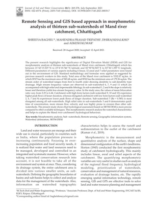
Fig. 1. Location of the study area (Mand river catchment)

RS AND GIS BASED MORPHOMETRIC ANALYSIS 271
July-September 2021]
Methodology
The topography information is required for the
delineation of the Mand river catchment and for
the preparation of drainage map.Adigital elevation
model (DEM) created from the data from the
Shuttle Radar Topography Mission (SRTM) has
been used in this analysis. The DEM was
downloaded from the website of the United States
Geological Survey (USGS), which was in the format
of Tagged Information File Format (TIFF), with
ground resolution of 30 m. Then, the developed
DEM was processed to delineate the Mand river
Catchment and to generate drainage network (Fig.
2) and thirteen sub-watersheds (Fig. 3), using the
Arc-Hydro extension tool of ArcGIS 10.5. For the
detailed and precise study, all the thirteen sub-
watersheds are studied individually. Hydrological
assessment based on SRTM DEM at catchment scale
is more applied and more accurate compared to
other available conventional techniques (Singh et
al., 2014). The designation of stream order is the
initial step in morphometric analysis based on the
hierarchical rendering of stream suggested by
Strahler (1964) which was used in the present
analysis. The fundamental parameters i.e., stream
number, stream length, area, perimeter and basin
length were derived in the platform of ArcGIS 10.5.
Morphometric analysis has been done for all the
thirteen sub-watersheds individually. The
formulaes for computation of the morphometric
parameters are shown in Table 1.
RESULTS AND DISCUSSION
Mand river catchment was divided into 13 sub-
watersheds whose statistics are tabulated in Table
2. Total area of the catchment is 5332.07 sq.km. with
perimeter of 589.73 km. It can be noticed from this
table that WS7 has the maximum area of 943.68
sq.km., whereas WS2 has the minimum area of
179.56 sq.km. The elevations of the sub-watersheds
varies from 187 m (MSL) to 1145 m (MSL). The
catchment has general slope towards north-east
direction with average elevation of 667 m above
MSL. The slope was classified in different classes.
The slope map of the Mand catchment (Fig. 5)
depicts the complex terrain with undulation and
irregular slopes. The various morphometric
parameters of the Mand river catchment area were
calculated and are tabulated in Tables 2-5.
The basic parameter of the Mand River
Catchment is shown in Table 1.
Software Used
ArcGIS 10.5 software was used for generating,
handling and creation of various layers and maps.
For mathematical calculations, the Microsoft excel
was used.
Linear Aspects
The linear aspects parameters were calculated
and results have been tabulated in Table 3.
Fig. 2. Drainage map
Fig. 3. Sub-watershed map

Table 2. Basic parameter of the Mand river catchment
Sr. Sub- Area (A) Perimeter (P) Area
no. Watershed (sq.km) (km) (%)
1 WS1 371.08 109.22 6.96
2 WS2 179.56 71.34 3.37
3 WS3 230.77 73.11 4.33
4 WS4 244.22 81.37 4.58
5 WS5 357.20 91.62 6.70
6 WS6 336.44 100.15 6.31
7 WS7 943.68 185.33 17.70
8 WS8 186.73 60.68 3.50
9 WS9 299.81 88.73 5.62
10 WS10 406.88 92.85 7.63
11 WS11 643.35 125.82 12.07
12 WS12 492.66 128.157 9.24
13 WS13 620.91 149.40 11.64
Table 1. Formulaes for computation of Morphometric parameters
Category of Name and Notation of Given equation References
parameter Morphometric Parameters
Linear parameters Stream Order Hierarchical Rank Strahler (1964)
Stream number (Nu) Nu = N1 + N2 + …+Nn Horton (1945)
Bifurcation ratio (Rb) Rb=Nu/Nu + 1 Schumm (1956)
Mean Bifurcation Ratio (Rbm) Rbm=Average of bifurcation Strahler (1964)
Basin length (Km) Obtained from Arc Map
Total stream Length (Km) Obtained from Arc Map
Areal parameters Area of the basin (A) (Km2
) Obtained from Arc Map
Basin Perimeter (P) (Km) Obtained from Arc Map
Form factor Ratio (Ff) Ff = A / Lb
2
Horton (1932)
Elongation Ratio (Re) Re= (2/ Lb )* 2"(A/ð) Schumm (1956)
Circularity Ratio (Rc) Rc = 4ð * A / P2
Miller (1953)
Drainage Density (Dd) (km/Km2
) Dd = Lu / A Horton (1932)
Texture ratio (T) T = Nu1 / P Horton (1932)
Stream Frequency (Fu) Fu = Nu / A Horton (1932)
Length of overland flow (Lo) Lo = ½ Dd Horton (1945)
Constant of channel maintenance (C) C = 1/Dd Horton (1945)
Shape index (Sw) Sw = Lb
2
/ A Horton (1932)
Compactness constant (Cc) Cc = 0.2824 * p/ “A Horton (1945)
Relief parameters Maximum Basin Height (m) GIS software analysis
Minimum Basin Height (m) GIS software analysis
Basin Relief (R) ( m) R= Max H – Min H Schumm (1956)
Relief Ratio (Rr) Rr = R / Lb Schumm (1956)
Relative Relief Ratio (Rhp) Rhp = H * 100/P Schumm (1956)
Drainage factor (Df) Df= Fu/Dd
2
Keshri and Rao (2018)
Ruggedness Number (Rn) Rn = Dd * (H / 1000) Patton and Baker (1976)
Stream Order (u)
The initial step in a drainage basin’s
geomorphological analysis is designating the
stream order; for this study, stream ordering given
by (Strahler, 1964) was used. Streams which emerge
from a source are named as streams of the first
order. When two first-order streams merge, an
order of two streams are formed, and so forth. The
order of a particular catchment is the order of the
highest stream of that catchment. Based on a
hierarchical ranking of streams, knowledge of
stream order number is beneficial in conjunction
with the size of its contributing catchment (Ansari
et al., 2012). On analysing drainage map, the Mand
River catchment was found to be of the 4th order
type, and the drainage pattern type is dendritic to
sub-dendritic. Physiography and structural state of
the research field are the significant factors
persuading the number of streams and order of
stream. The drainage map showing stream orders
of the Mand river catchment is presented in Fig. 4.
Stream Number (Nu)
It is the total number of streams of different
orders, which is inversely proportional to the order
of streams. As the order increases, the number of
stream of that order decreases, and the higher
stream order implies less permeability and
infiltration. The variation in the stream order and
size of the tributary catchments largely depends on
the catchment’s physiographical, geomorpho-
logical, and structural properties (Khanday and
Javed, 2016). The hydrological character of the basin
area is extremely important as it offers significant
information on surface runoff variables. The much

Total stream length (Lu)
The lengths of the different stream segments
are calculated using GIS tools. All thirteen sub-
watersheds shows that the total length of stream
segments is maximum in the first-order streams and
decreases as the order of stream increases. It is one
of the most important hydrological features, as it
provides information on surface runoff
characteristics. The short length of the river
indicates typical regions with steep slopes and good
texture. Rivers that have slightly longer lengths are
usually indicative of smoother slope (Radwan et al.,
2017). The length shows the temporal evolution of
a streams that deals with tectonic disorders. The
number and length of streams vary depending
directly on the size of the sub-watersheds. Total
stream length which is shown in Table 3 are the
summation of stream length of all the orders in the
respective sub-watershed (Prasad et al., 2020). Sub-
watershed WS7 has the longest stream length (Lu
= 2091.41 km), while sub-watershed WS2 has the
minimum Lu value of 350.96 km.
Basin Length (Lb
)
Schumm (1956) described the length of the
basin as the longest dimensional parallel to the main
drainage line. Gregory (1978) defined the basin
length to be the longest basin length of which the
mouth is one end. Gardiner (1978) described the
length of the basin as the length of a basin line in
any direction from the mouth of sub-watershed to
a point on the sub-watershed perimeter equidistant
from the mouth. The main stream is identified by
starting from the basin outlet and moving up the
catchment.At any branching point the largest order
branch is taken. If there is a branch of two streams
of the same order, the one with the largest
catchment area is taken as the main stream. Sub-
watershed WS7 has the longest basin length i.e.
59.29 km.
Bifurcation Ratio (Rb)
Bifurcation ratio which is a dimensional less
quantity is the ratio of number of streams of the
given order u to the total number of streams of
higher order u+1 given by Schumn (1956). Horton
(1945) considered the bifurcation ratio as relief
index and dissection index. In general, lower Rb
value is characteristics of a catchment that have
experienced fewer structural disturbances and
structural disturbances have not disrupted the
drainage pattern. Abnormally high Rb values
predict steeply dipping rock layers in region. The
Fig. 4. Stream order Map
Fig. 5. SlopeMap
smaller river is the physiognomy of regions with
steep gradients and better textures. Total number
of streams as given in Table 3 are the summation of
stream numbers of all the orders in the respective
sub-watershed. Maximum number of streams i.e.
3983 was found in WS7 whereas minimum was 467
i.e. in WS2. The maximum first order stream
numbers shows the intensity of the area’s
permeability and infiltration features.

Rb value is also representative of basin shape. The
bifurcation ratio indicates a limited variation range
for various regions or for various ecosystems except
where strong geological influence prevails (Kumar
et al., 2016). Mean Bifurcation ratio (Rbm) is the
mean of all the bifurcation ratios of the respective
watershed. The Mean Bifurcation ratio can be
observed from Table 3 that it is distinct from one
another. An elongated basin have high Rbm (SW2,
SW4, and SW7), where as a circular basin have a
low Rbm (SW8, SW9 and SW13). These
irregularities depends on the drainage basin’s
geological and lithological development (Strahler,
1964). The values of Rbm ranges from 2.25 to 6.44
(Table 3), in the study area. Normally, when the ‘Rb’
value is low, the basin produces a sharp discharge
peak while the basin produces a low but prolonged
peak flow during high Rb value.
Areal Aspects
The values of the areal parameters were
determined and results were given in Table 4 for
all thirteen sub-watersheds. A remarkable relation
between the total sub-watershed areas and the total
stream lengths supported by the contributing areas
has been recognized by Schumm (1956).
Drainage Density (Dd
)
The ratio of overall stream length of all the
orders of the basin to basin area is known as
drainage density (Horton, 1932). Dd measured in
km/km2 shows the closeness of channel spacing and
is a quantitative indicator of the average stream
channel length for the entire basin. It also provides
an understanding of the characteristics of the rocks
that underlie it. Low drainage density occurs in
areas of dense vegetation, low relief with highly
resistant and permeable sub-soil layer, while high
drainage density exists in the region of
impermeable, porous sub-soil layer with low
vegetation and high relief (Strahler, 1964). The
drainage density is managed by various variables
including relief, rainfall, terrain infiltration
capability and land erosion resistance (Horton,
1945). Drainage density varies between 1.96 to 2.43
in the study area (Table 4).
Stream frequency / Drainage frequency (Fu)
Stream frequency or drainage frequency (Fu)
is the cumulative number of stream segments of
all the orders per unit area given by Horton (1932).
The Fu is inversely related to infiltration and is
directly connected to roughness of the catchment.
This depends primarily on the geology of the
catchment and represents the texture of the
drainage network. Higher stream frequencies
demonstrate the early phases of the fluvial process
or restored erosional activities along the steep
slopes. In sub-watersheds 6, 7, 9 and 11 high Fu
values are observed which shows high relief and
impermeability in geology. The slope is
comparatively lower in sub-watersheds 1, 2 and 4
and therefore it yields lower value of Fu.
Form Factor (Ff
)
The form factor (Ff) may be specified, according
to Horton (1932), as the ratio of the basin area to
the basin length square. The form factor shows the
Table 3. Linear parameter of the Mand river catchment
Sr. no. Sub-watershed Total number Total stream Basin length Mean
of streams length (Lu) (Lb) bifurcation
(Nu) (km) (km) ratio (Rbm)
1 WS1 1169 757.65 35.84 4.25
2 WS2 467 350.96 21.05 6
3 WS3 732 490.73 21.18 3.13
4 WS4 821 480.84 26.63 6
5 WS5 1232 760.53 26.23 4.5
6 WS6 1324 696.11 30.39 3.5
7 WS7 3983 2091.41 59.29 6.44
8 WS8 574 388.15 23.60 2.25
9 WS9 1321 722.10 21.41 2.84
10 WS10 1409 874.63 26.68 4.17
11 WS11 3023 1563.83 39.49 4.42
12 WS12 1854 1014.02 29.07 4.24
13 WS13 2294 1460.20 33.89 2.98

flow intensity for a defined area of the catchment.
This is a dimensionless characteristic, which is used
as a numerical representation of the catchment
shape. Smaller the form factor, more elongated will
the catchment. Sub-watersheds with higher values
of form factors (sub-watershed 9, 10 and 12) have
higher peak flows of lesser duration, whereas
elongated catchment with low values of form
factors (sub-watershed 2,6,7 and 8) have lesser peak
flows of higher duration. Table 4 shows values of
form factor for different sub-watersheds.
Circulatory Ratio (Rc)
Reddy et al. (2004) stated the dimensionless
circularity ratio (Rc) as the ratio of the catchment
area to the area of circle having equal perimeter as
the catchment. Rc is influenced by stream length,
drainage frequency, geology, land use, land cover,
relief, basin climate and slope. Lower Rc value
shows that catchment is elongated. Rc values close
to 1 reveals that the catchment is circular, giving
rise to uniform absorption and excess water takes
longer duration to reach at the outlet of the basin
(Kumar et al., 2014). Circulatory ratio of all the sub-
watersheds are tabulated in Table 4. The sub-
watershed WS7 has lowest value (0.35) while sub-
watershed WS8 has highest value (0.64). The ‘Rc”
low, medium and high values indicate the young,
mature, and old phases of the tributary watershed’s
life cycle.
Elongation Ratio (Re)
The elongation ratio (Re) is the ratio with the
diameter of the circle of the same area as that of the
catchment to the average basin length (Schumm,
1956). Generally, Re values ranges from 0.6 to 1.0
over a wide variation in climatic and geological
conditions. Values close to 1.0 are indicative of low
relief areas, while values in the 0.6–0.8 range reveals
high relief and steep ground slope (Strahler, 1964).
It is possible to divide such values into three types:
(i) circular (Re > 0.9), (ii) oval (0.9–0.8), (c) elongated
(Re < 0.8). This index shows higher significance in
catchment shape analysis which helps to offer an
idea of a drainage basin’s hydrological character.
For runoff discharge, a circular catchment is more
productive than an elongated catchment. SW7 (Re
= 0.59) is most elongated among all sub-watersheds.
Values of Re of thirteen sub-watersheds is presented
in Table 4.
Length of Overland Flow (Lo)
Lo is stated as non-stream flow from a point on
catchment boundary to the adjacent stream. Since
at an average this length of overland flow is about
half the distance between the stream channels
(Horton, 1945), for convenience’s sake, had taken it
to be about half the reciprocal of drainage density.
It is an independent parameter which affects both
the catchment’s hydrological and physiographic
development. For steeper slopes this parameter is
lower, and for mild slopes its higher. It affects both
the process of runoff and of flooding. The overland
flow and surface runoff are slightly dissimilar, the
overland flow is that flow of precipitated water that
passes over the surface of the earth reaching the
streams, while the river flow that reaches the outlet
of the catchment is stated as surface runoff. For
Table 4. Aerial Aspect of the Mand River Catchment
S. Sub- Drainage Stream Length of Texture Circulatry Form Shape Elongation Compact- Constant
no. watershed density frequency overland ratio ratio factor factor ratio ness of channel
(Dd) (Fu) flow (Lo) (T) (Rc) (Rf) (Bs) (Re) constant mainten-
(Cc) ance (C)
1 WS1 2.04 3.15 1.02 10.70 0.39 0.29 3.46 0.61 1.60 0.49
2 WS2 1.96 2.60 0.98 6.55 0.44 0.40 2.47 0.72 1.50 0.51
3 WS3 2.13 3.17 1.06 10.01 0.54 0.52 1.94 0.81 1.36 0.47
4 WS4 1.97 3.36 0.98 10.09 0.46 0.34 2.90 0.66 1.47 0.51
5 WS5 2.13 3.45 1.07 13.45 0.53 0.52 1.93 0.81 1.37 0.47
6 WS6 2.07 3.94 1.04 13.22 0.42 0.36 2.74 0.68 1.54 0.48
7 WS7 2.22 4.22 1.11 21.49 0.35 0.27 3.73 0.59 1.70 0.45
8 WS8 2.08 3.07 1.04 9.46 0.64 0.34 2.98 0.65 1.25 0.48
9 WS9 2.41 4.41 1.20 14.89 0.48 0.65 1.53 0.91 1.45 0.42
10 WS10 2.15 3.46 1.08 15.18 0.59 0.57 1.75 0.85 1.30 0.47
11 WS11 2.43 4.70 1.22 24.03 0.51 0.41 2.42 0.73 1.40 0.41
12 WS12 2.06 3.76 1.03 14.47 0.38 0.58 1.72 0.86 1.63 0.49
13 WS13 2.35 3.70 1.18 15.36 0.35 0.54 1.85 0.83 1.69 0.43

smaller watersheds, the overland flow is dominant
than in the larger watersheds. Low values of Lo are
observed in sub-watersheds 1, 2, 4, 12 and 6, which
represents high relief and steep slope. In contrast,
sub-watersheds 9, 11 and 13 have higher Lo values
with relatively low relief and average slope. Sub-
watershed WS11 has maximum (1.21 km) and sub-
watershed WS2 has minimum (0.98 km) length of
overland flow (Lo) among 13 sub-watersheds (Table
4).
Constant of channel maintenance (C)
Constant of channel maintenance is the reverse
of Dd (Horton, 1945). It analyse square unit number
of river catchment area required to maintain a unit
of linear stream channel. Plain area requires a wide
area of catchment surface to maintain a single
channel unit than hilly region (Strahler, 1952). In
study basin, the highest C value i.e., 0.512 exist in
sub-watershed WS2 and the lowest i.e., 0.41 in sub-
watershed WS11 (Table 4). High C value shows that
the sub-watersheds area of lower order streams are
relatively larger than the sub-watersheds which
have lower C value. Lower C values minimizes Lo,
thus quickly water get discharge as channel flow
under very scant vegetative cover. This indicator
represents the flow control and infiltration at the
outlet of catchment.
Texture ratio (T)
Texture ratio is the significant parameter in the
morphometric study which depends on the terrain’s
underlying geology, soil infiltration capacity and
relief of catchment. It is defined as the ratio of total
number of 1st order streams to the perimeter of
catchment. The sub-watershed WS11 has maximum
(T=24.03), while sub-watershed WS2 has minimum
(T=6.55). The values of the all sub-watershed’s
texture ratio is shown in Table 4.
Compactness constant (Cc)
The Cc is directly related to the capacity to
infiltrate. The Cc is independent of catchment size
and reliant only on the slope. The sub-watershed
WS7 has highest value (Cc = 1.70), while sub-
watershed WS8 has lowest value (Cc =1.25) with
low permeability. The values of the Cc are shown
in Table 4.
Shape index (Sw)
The shape index of the catchment is equal to
the square of the basin length divided by the area
of the catchment (Horton, 1932). The Sw of the
drainage basin along the length and relief affects
the rate of flow of water and sediment yield. The
sub-watershed WS7 has maximum (Sw = 3.73),
while sub-watershed WS9 has minimum (Sw =
1.53). The values of the shape index of thirteen sub-
watersheds are tabulated in Table 4.
Relief Aspects
The elevations of the sub-watersheds in the
present study ranges from 187 m to 1145 m (MSL).
The Relief aspects parameters have been computed
and results were tabulated in Table 5.
Basin Relief (R)
The maximum vertical distance between the
lowest and highest point of the catchment is the
Table 5. Relief aspect of the Mand river catchment
S. no. Sub-watershed Max Basin Min Basin Basin Ruggedness Drainage Relative Relief
height height relief number factor relief ratio
1 WS1 1145 272 873.00 1.78 0.76 0.80 0.02
2 WS2 730 493 237.00 0.46 0.68 0.33 0.01
3 WS3 1027 269 758.00 1.61 0.70 1.04 0.04
4 WS4 652 256 396.00 0.78 0.87 0.49 0.01
5 WS5 1013 248 765.00 1.63 0.76 0.83 0.03
6 WS6 821 235 586.00 1.21 0.92 0.59 0.02
7 WS7 820 222 598.00 1.33 0.86 0.32 0.01
8 WS8 990 248 742.00 1.54 0.71 1.22 0.03
9 WS9 858 240 618.00 1.49 0.76 0.70 0.03
10 WS10 814 215 599.00 1.29 0.75 0.65 0.02
11 WS11 606 187 419.00 1.02 0.80 0.33 0.01
12 WS12 1105 495 610.00 1.26 0.89 0.48 0.02
13 WS13 1139 568 571.00 1.34 0.67 0.38 0.02

total relief (Patton and Baker, 1976). It is also called
Basin relief (R). It determines the stream channel
gradient, and thus affects flood patterns and the
sediment amount that gets transported. This is the
measure of a drainage system’s potential energy,
provided by the elevation. R value ranges between
237 m in SW2 and 873 m in SW1. Sub-watersheds
2, 4 and 11 have low relief (R < 500 m) (Table 5). On
increasing relief, steeper hillsides and higher stream
gradients, concentration time decreases, thus flood
peaks increase (Patton and Baker, 1976).
Relief Ratio (Rr)
The relief ratio is the ratio between a basin relief
to longest dimension of the catchment parallel to
the main drainage line (Schumn, 1956). This is a
dimensionless entity and is very beneficial when
there is a lack of knowledge of topography. In
catchment, the values of relief ratio varies from 0.01
to 0.04 (Table 5). Areas with steep slope and high
relief were associated with high Rr values. Less Rr
values were attributed primarily to the catchment’s
more impenetrable basement rocks and very low
degree of slope. Relief ratio (Rr) measures the total
steepness of the catchment and is significant
predictor of the strength of the erosion processes
that functions as a result of the slope. High Rr in
sub-watersheds 3 and 8 shows quick time of
concentration and rate of stream flow and is
vulnerable to erosion than other sub-watersheds.
Relative Relief (Rhp
)
Relative Relief is the ratio of the maximum
catchment relief to the perimeter of the catchment
(Schumn, 1956). Relative relief will effectively
present the relief characteristics without taking into
account the sea level (Miller, 1953). The value of
the Rhp for 13 sub- watersheds are shown in Table
5. Sub-watershed WS7 has lowest Rhp (0.32), while
sub-watershed WS8 had the highest value of Rhp
(1.22).
Ruggedness number (Rn)
Ruggedness number is a dimensionless
parameter that is calculated by the product of R
and Dd where both are in the same units (Kumar et
al., 2018). Rn is used to calculate the flood potential
of streams. Extremely high value of Rn exists when
both variables are more, i.e. when slope is not only
steep but long as well. In Mand catchment, Rn value
ranges between 0.46 to 1.78 (Table 5). Sub-
watersheds 2, 4 and 11 have low Rn values whereas
rest of the sub-watersheds showed high Rn value.
The high Rn values represent the complex
structures of a landscape which is highly prone to
erosion. The Rn is directly linked to erodibility,
increasing erosivity increases with Rn. The high
relief areas and low Dd are rough as low relief areas
with high Dd. Ahigh value of Rn would bring about
a sudden rise in the hydrograph.
Drainage factor (Df)
Drainage factor (Df) is defined as the ratio of
Fu to the square of Dd. In catchment, Df value varies
between 0.67 and 0.92 (Table 5).
CONCLUSIONS
The study showed that the GIS-based approach
is more appropriate than traditional methods in
assessing morphometric parameters at river
catchment level. The quantitative morphometric
analysis was carried out in thirteen sub-watersheds
of Mand river catchment. The slope map of the
Mand catchment depicts the complex terrain with
undulation and irregular slopes. The stream order
of watershed ranges from first to fourth order
showing dendritic to sub-dendritic type drainage.
In the study area, the values of mean bifurcation
ratio vary from 2.25 to 6.44. High relief ratio in sub-
watersheds 3 and 8 indicates quick time of
concentration, stream flow velocity and highly
prone to erosion than other sub-watersheds. The
value of ruggedness number (Rn) value ranges
between 0.463 and 1.782. The morphometric study
of various sub-watersheds reveals its relative
characteristics with respect to the watershed’s
hydrological response. The hydrological activity of
the Mand catchment in the downstream area of the
catchment would have a profound effect on the
vulnerability to flooding and erosion by observing
Mand catchment morphometry, the shift in
discharge variation shows that the dynamism of
river morphology is the result of natural processes
and anthropogenic interference as well.
REFERENCES
Ansari, Z.R., Rao, L.A.K. and Yusuf, S. 2012. GIS based
morphometric analysis of Yamuna drainage network
in parts of Fatehabad area of Agra district, Uttar
Pradesh. Jour. Geol. Soc. India 79(5): 505-514.
Gardiner, V. 1978. Redundancy and spatial organization of
drainage basin form indices. Transactions of the Institute
of British Geographers, New Series 3: 416-431.
Gregory, K.J. 1978. Fluvial Processes in British Basins, in:
C. Embleton, D, Brunsden and D.K.C. Jones (ed)
Geomorphology- present problems and future
prospects. OUP, NY, pp. 40-72.

Horton, R.E. 1932. Drainage basin characteristics. Trans.
Amer. Geophys. Union 13: 350-361.
Horton, R.E. 1945. Erosional development of streams and
their drainage basins: hydrophysical approach to
quantitative morphology. Bull. Geo. Soc. Am. 56: 275-
370.
Kabite, G. and Gessesse, B. 2018. Hydro-geomorphological
characterization of Dhidhessa River Basin, Ethiopia.
Int. Soil Water Conserv. Res. 6: 175-183.
Kaushik, P. and Ghosh, P. 2018. Morphometric analysis of
Shipra River sub-basin, India, remote sensing and GIS
approach. Int J. Creat Res. Thoughts 6(1): 1536-1546.
Khanday, M.Y. and Javed, A. 2016. Prioritization of sub-
watersheds for conservation measures in a Semi-arid
watershed using remote sensing and GIS. Journal of
Geological Society of India 88(2): 185-196.
Kumar, A., Samuel, S.K. and Vyas, V. 2014. Morphometric
analysis of six sub-watersheds in the central zone of
Narmada River. Arab J. Geosci. 8(8): 5685-5712.
Kumar, D., Singh, D.S., Prajapati, S.K., Khan, I., Gautam,
P.K. and Vishwkarma, B. 2018. Morphometric
parameters and neotectonics of Kalyani river basin,
Ganga plain: Aremote sensing and GIS approach. Jour.
Geol. Soc. India 91: 679-686.
Kumar, L., Khalkho, D., Pandey, V.K., Tripathi, M.P. and
Singh, P. 2019. Sub watershed characterization and
prioritization using geoinformatics for natural
resources management. Journal of Soil and Water
Conservation 18(4): 342-353.
Kumar, V.R., Venkatesh, A.S., Janapriya, S., Rajasekar, M.
and Muthuchamy, I. 2016. Morphometric analysis and
prioritization of Palathodi watershed in Parambikulam-
Aliyar basin, Tamil Nadu using RS and GIS. Asian
Journal of Environmental Science 11(1): 51-5S8.
Miller, V.C. 1953. A quantitative geomorphologic study of
drainage basin characteristics in the Clinch mountain
area, Virginia and Tennessee, Project NR 389042, Tech
Rept 3. Columbia University Department of Geology,
ONR Geography Branch, New York.
Naitam, R.K., Singh, R.S., Sharma, R.P., Verma, T.P. and
Arora, Sanjay 2016. Morphometric analysis of
Chanavada-II watershed in Aravalli hills of southern
Rajasthan using geospatial technique. Journal of Soil and
Water Conservation 15(4): 318-324.
Patton, P.C. and Baker, V.R. 1976. Morphometry and floods
in small drainage basins subject to diverse
hydrogeomorphic controls. Water Resour Res. 12: 941-952.
Prakash, K., Mohanty, T., Singh, S., Chaubey, K. and
Prakash, P. 2016. Drainage morphometry of the Dhasan
river basin, Bundelkhand craton, central India using
remote sensing and GIS techniques. J. Geomat 10: 21-132.
Prakash, K., Singh, S. and Shukla, U.K. 2016. Morphometric
changes of the Varuna river basin, Varanasi district,
Uttar Pradesh. J. Geom. 10: 48-54.
Prasad, V., Yousuf, A., and Sharma, N. 2020. GIS based
morphometric analysis of a forest watershed in lower
Shivaliks of Punjab using high resolution satellite data.
Journal of Soil and Water Conservation 19(3): 292-299.
Radwan, F., Alazba, A.A. and Mossad, A. 2017. Watershed
morphometric analysis of Wadi Baish Dam catchment
area using integrated GIS-based approach. Arabian J.
of Geosciences 10(12): 256.
Reddy, G.P.O., Maji, A.K. and Gajbhiye, K.S. 2004. Drainage
morphometry and its influence on landform
characteristics in a basaltic terrain, Central India – a
remote sensing and GIS approach. Int. J. Appl. Earth
Obs Geoinf. 6: 1-16.
Schumn, S.A. 1956. Evaluation of drainage systems and
slopes in badlands at Perth Amboy, New Jersy. Geol.
Soc. Am. Bull. 67: 597-646.
Singh, P., Gupta, A. and Singh, M. 2014. Hydrological
inferences from watershed analysis for water resource
management using remote sensing and GIS techniques.
Egypt J Remote Sens Space Sci. 17: 111-121.
Strahler, A.N. 1952. Dynamic basis of geomorphology. Bull
Geol. Soc. Am. 63: 923-938.
Strahler,A.N. 1964. Quantitave geomorphology of drainage
basins and channel networks In. Handbook of Applied
Hydrology, McGraw Hill Book Company, New York,
Section 4-II.
Strahler, A.N. 1968. Physical Geography, 3rd Edition,
Chapter 29, Quantative analysis of erosional landform.
Thakur, K.K., Pandita, S.K., Goyal, V.C., Arora, Sanjay,
Kotwal, S.S. and Singh, Y. 2012. GIS based approach
for prioritization of Balwal watershed, Jammu, Jammu
and Kashmir. Himalayan Geology 33(2): 151-161.
Verma, A.K. and Jha, M.K. 2017. Extraction of watershed
characteristics using GIS and digital elevation model.
International Journal of Engineering Science Invention 6(7):
01-06.
Zolekar, R.B. and Bhagat, V.S. 2015. Multi-criteria land
suitability analysis for agriculture in hilly zone: Remote
sensing and GIS approach. Comput Electron Agric. 118:
300-321.

04 mb.v.h

Recommended

Recommended

More Related Content

What's hot

What's hot (19)

Similar to 04 mb.v.h

Similar to 04 mb.v.h (20)

Recently uploaded

Recently uploaded (20)

04 mb.v.h