This document provides a summary report of a research study combining multivariate control charts and neural networks to estimate the starting time of process disturbances. The study was conducted by graduate students at Fu Jen Catholic University under the guidance of Dr. Shao Yuehjen. The research aims to address the limitations of traditional univariate and multivariate control charts in identifying the starting point of process faults by leveraging the computational abilities of neural networks. The study develops theoretical frameworks for combining multivariate control charts with neural networks and conducts simulation experiments to demonstrate the advantages of the proposed approach over using control charts alone. The results show the combined method can more accurately and earlier detect the starting fault point, helping reduce costs and resume normal operations.

1. I
天主教輔仁大學統計資訊學系
第五屆專題研究成果報告
指導老師：邵曰仁
應用多變量管制圖與類神經網路
以估計多變量製程出錯啟始時間之研究
Combining Multivariate Control Charts and
Neural Networks to Estimate the Starting Time
of a Process Disturbance
研究學生：鍾宇婷 陳玫君
陳玉霞 吳孟芸
劉宥听 高益信 撰
中華民國九十四年十二月

2. I
摘要
論文題目：應用多變量管制圖與類神經網路以估計多變量製程出錯啟
始時間之研究
校(院)系所組別：輔仁大學管理學院統計資訊學系
研究成員：鍾宇婷、陳玫君、陳玉霞、吳孟芸、劉宥听、高益信
指導教授：邵曰仁 博士
論文頁數：101 頁
關鍵詞：SPC 管制圖、多變量管制圖、類神經網路、出錯啟始
點
社會大眾對於品質的要求越來越高，而市面上之商品也大都具有多重品質特
性，所以不論在學術研究或實務應用上，生產線的品管技術都逐漸朝向監控多重
品質特性的方向發展。目前業界大都使用單變量管制圖監控製程，只能偵測單一
品質特性，對於具有多個品質特性的產品而言，使用單變量管制圖進行監控分析
將費時又消耗龐大成本。然而，多變量 SPC 管制圖雖可一次監測多重品質特性，
但仍無法有效找出製程之出錯啟始點。本文將探討應用類神經網路強大的運算及
分析能力，結合多變量 SPC 管制圖找出製程出錯啟始點。期望經由結合多變量 SPC
管制圖及類神經網路的優點後，相較於只使用多變量 SPC 管制圖時，能大幅提前
且正確判斷製程出錯啟始點。若幫助企業節省下找尋製程啟始出錯點時所必須耗
費的成本，將可有效降低成本以及幫助製程在發現錯誤後，以最短的時間恢復正
常運作。本文將詳細探討多變量 SPC 管制圖與類神經網路結合之理論架構，找出
在不同管制圖下，單純使用 SPC 管制圖與結合類神經網路分析數據後，可較單純
使用 SPC 管制圖提前多少時間點找出起始出錯點，並進行實驗佐以證明本文提出
方法之優勢與未來展望。

3. II
Abstract
Title of Thesis: Combining Multivariate Control Charts and Neural Network to
Estimate the Starting Time of a Process
Name of Institute: Department of Statistics and Information Science, College of
Management, Fu Jen Catholic University
Name of Student: Chung Yu Ting, Chen Mei Chun, Chan Iok Ha, Wu Meng Yun,
Lu you Ying, Kao Yi Shin
Advisor: Shao Yuehjen E.
Total Pages: 101pages
Key words: Multiple Quality Characteristics, Multivariate Control
Chart, Neural Network
Abstract:
Because of rapid advances in technology, consumers have higher concern for the
quality of products than ever before. There are many aspects of quality in each
product, so quality control techniques in production should pay attention to monitoring
multiple characteristics. Nowadays, most of the process personnel use univariate
control charts to monitor the process which can detect the single quality characteristic.
As for products which have more quality characteristics, it only wastes time and money
to use univariate control charts. Multivariate control charts can simultaneously
monitor many quality characteristics, although one cannot effectively find out the
staring fault point. In our research, we will discuss the combination of multivariate
control charts and Neural Networks (NN), which have great computing and analysis
capability, to find out the starting fault point. We expect that through combining the

4. III
multivariate control chart and NN, we can find out the starting fault point in advance by
comparing by checking it against the multivariate control chart. Provided that can
eliminate the errant production, this will decrease costs and resume the normal process
in a short time. We will discuss more deeply the construction of multivariate control
chart in combination with NN and do the experiment to prove the advantages of the
proposed method.

5. I
CONTENTS
CONTENTS ..................................................................................................................I
LIST OF TABLES.........................................................................................................IV
LIST OF FIGURES.......................................................................................................VII
Chapter 1 INTRODUCTION .....................................................................................1
1.1 Motivation .......................................................................................................1
1.2 Research Flow .................................................................................................4
Chapter 2 LITERATURE REVIEW...........................................................................8
2.1 Hotelling 2
T Control Chart...........................................................................8
2.2 MEWMA Control Chart..................................................................................9
2.3 Neural Network ...............................................................................................10
Chapter 3 RESEARCH APPROACH ........................................................................12
3.1 Description of the Problem (1) ......................................................................12
3.1.1 Univariate Control Chart ......................................................................12
3.1.2 Weaknesses of the Univariate Control Chart........................................13
3.2 Description of the Problem (2) ......................................................................16
3.2.1 Hotelling 2
T Control Chart................................................................16
3.2.2 MEWMA Control Chart.......................................................................19
3.2.3 Weaknesses of the Multivariate Control Chart.....................................21
3.3 Description of the Approach............................................................................24
3.3.1 Binomial Distribution...........................................................................24
3.3.2 Neural Networks (NN) .......................................................................27
3.4 Test Process and the Result..............................................................................29

6. II
3.4.1 Constructing NN Model .......................................................................30
Chapter 4 SIMULATION STUDIES AND ANALYSIS............................................36
4.1 Combination of Hotelling 2
T Control Chart and Neural Networks.. ..........36
4.1.1 p=3........................................................................................................37
4.1.2 p=5........................................................................................................40
4.1.3 p=8........................................................................................................43
4.1.4 p=12......................................................................................................46
4.1.5 Analysis ................................................................................................50
4.2 Combination of MEWMA Control Chart and Neural Networks...................51
4.2.1  =0.1 ..................................................................................................51
4.2.1.1 p=2...............................................................................................51
4.2.1.2 p=4...............................................................................................53
4.2.1.3 p=6...............................................................................................55
4.2.1.4 p=10.............................................................................................57
4.2.2  =0.2 ..................................................................................................60
4.2.2.1 p=2...............................................................................................60
4.2.2.2 p=4...............................................................................................62
4.2.2.3 p=6...............................................................................................64
4.2.2.4 p=10.............................................................................................66
4.2.3  =0.3 ..................................................................................................69
4.2.3.1 p=2...............................................................................................69
4.2.3.2 p=4...............................................................................................71
4.2.3.3 p=6...............................................................................................73
4.2.3.4 p=10.............................................................................................75
4.2.4  =0.4 ..................................................................................................78

7. III
4.2.4.1 p=2...............................................................................................78
4.2.4.2 p=4...............................................................................................80
4.2.4.3 p=6...............................................................................................82
4.2.4.4 p=10.............................................................................................84
4.3 Comparison of MEWMA Control Charts with Same Quality Characteristics
but Different  Values................................................................................87
4.3.1 p=2........................................................................................................88
4.3.2 p=4........................................................................................................88
4.3.3 p=6........................................................................................................89
4.3.4 p=10......................................................................................................89
4.4 Comparison and Contrast of the Result of Hotelling 2
T Control Chart and
MEWMA Control Chart................................................................................90
Chapter 5 CONCLUSIONS AND FUTURE RESEARCH........................................93
5.1 Conclusions .............................................................................................................93
5.2 Future Research.............................................................................................96
REFERENCES..............................................................................................................98

8. IV
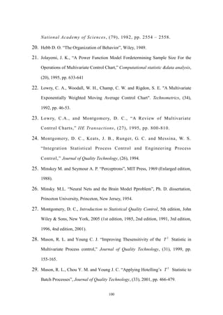
LIST OF TABLES
Table 3-1 RMSE for different numbers and learning rates..........................................32
Table 3-2 The correct determine rate in every threshold value ...................................33
Table 3-3 Example testing data ...................................................................................35
Table 4-1 The learning rate and RMSE of ]0,0,1[1  and p=3...............................39
Table 4-2 The threshold value and the correct determine rate of ]0,0,1[1  and p=3
....................................................................................................................39
Table 4-3 The models in different shifts of p=3 ..........................................................40
Table 4-4 The different starting fault points of p=3 in every Prob..............................40
Table 4-5 The models in different shifts of p=5 ..........................................................42
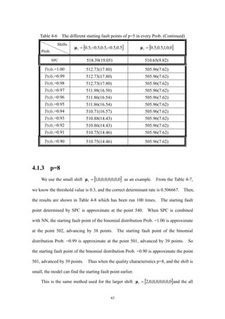
Table 4-6 The different starting fault points of p=5 in every Prob..............................42
Table 4-7 The models in different shifts of p=8 ..........................................................45
Table 4-8 The different starting fault points of p=8 in every Prob..............................45
Table 4-9 The models in different shifts of p=12 ........................................................48
Table 4-10 The different starting fault points of p=12 in every Prob..........................48
Table 4-11 The small shift outcomes in different quality characteristics
of Hotelling 2
T .......................................................................................51
Table 4-12 The models in different shifts of p=2 and  =0.1 ....................................53
Table 4-13 The different starting fault points of p=2 and  =0.1in every Prob.........54
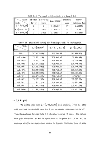
Table 4-14 The models in different shifts of p=4 and  =0.1 ....................................55
Table 4-15 The different starting fault points of p=2 and  =0.1in every Prob.........56
Table 4-16 The models in different shifts of p=6 and  =0.1 ....................................57
Table 4-17 The different starting fault points of p=6 and  =0.1in every Prob.........58

9. V
Table 4-18 The models in different shifts of p=10 and  =0.1 ..................................60
Table 4-19 The different starting fault points of p=10 and  =0.1 in every Prob......60
Table 4-20 The models in different shifts of p=2 and  =0.2 ....................................62
Table 4-21 The different starting fault points of p=2 and  =0.2 in every Prob........63
Table 4-22 The models in different shifts of p=4 and =0.2 ......................................64
Table 4-23 The different starting fault points of p=4 and  =0.2in every Prob...........65
Table 4-24 The models in different shifts of p=6 and  =0.2 ....................................66
Table 4-25 The different starting fault points of p=6 and  =0.2 in every Prob........67
Table 4-26 The models in different shifts of p=10 and  =0.2 ..................................69
Table 4-27 The different starting fault points of p=10 and  =0.2 in every Prob........69
Table 4-28 The models in different shifts of p=2 and =0.3 ......................................71
Table 4-29 The different starting fault points of p=2 and  =0.3 in every Prob..........72
Table 4-30 The models in different shifts of p=4 and  =0.3 ....................................73
Table 4-31 The different starting fault points of p=4 and  =0.3in every Prob.........74
Table 4-32 The models in different shifts of p=6 and  =0.3 ....................................75
Table 4-33 The different starting fault points of p=6 and  =0.3 in every Prob........76
Table 4-34 The models in different shifts of p=10 and  =0.3 ..................................78
Table 4-35 The different starting fault points of p=10 and  =0.3 in every Prob........78
Table 4-36 The models in different shifts of p=2 and  =0.4 ....................................80
Table 4-37 The different starting fault points of p=2 and  =0.4 in every Prob........81
Table 4-38 The models in different shifts of p=4 and  =0.4 ....................................82
Table 4-39 The different starting fault points of p=4 and  =0.4 in every Prob........83
Table 4-40 The models in different shifts of p=6 and  =0.4 ....................................84
Table 4-41 The different starting fault points of p=6 and  =0.4 in every Prob..........85
Table 4-42 The models in different shifts of p=10 and  =0.4 ..................................87

10. VI
Table 4-43 The different starting fault points of p=10 and  =0.4 in every Prob......87
Table 4-44 The different  outcomes when p=2 ......................................................89
Table 4-45 The different  outcomes when p=4 ......................................................89
Table 4-46 The different  outcomes when p=6 ......................................................90
Table 4-47 The different  outcomes when p=10 ....................................................91
Table 4-48 Comparison of Hotelling 2
T and MEWMA（Considering
p and the shift are small）........................................................................92
Table 4-49 Comparing of Hotelling 2
T and MEWMA（Considering p is larger but the
shift are small） .......................................................................................93
Table 5-1 Different shift outcomes when using Hotelling 2
T control chart in
combination with NN .................................................................................95
Table 5-2 Different shift outcomes when using MEWMA control chart
in combination with NN ( =0.2 and 0.3)..................................................96

11. VII
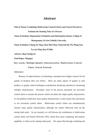
LIST OF FIGURES
Figure 1-1 Research flow .............................................................................................4
Figure 3-1 Univariate control charts---the mean-standard deviation control chart....13
Figure 3-2 Control ellipse ( 1X , 2X are independent variables)..............................14
Figure 3-3 Control ellipse ( 1X , 2X are dependent variables).................................15
Figure 3-4 The shift 0 = [1, 0, 0] of Hotelling 2
T control chart.............................22
Figure 3-5 The shift 1 =[0.5,0,0] of Hotelling 2
T control chart .............................23
Figure 3-6 The basic construction of NN...................................................................28
Figure 3-7 The process of constructing NN model ....................................................30
Figure 3-8 RMSE trend chart .....................................................................................31

12. 1
Chapter 1 INTRODUCTION
1.1 Motivation
Production quality has become very important due to competitive and global
markets. Because of increases in average national income, consumers have begun to
seek increased quality of life and consumer demand increased. The level of production
quality itself has been turning into the prime concern of the business world. As new
products emerge, the rate of product elimination increases as well. People now care less
about price than about the quality of their products. Products with better quality will
sell better as consumers are more willing to purchase high quality goods. So suppliers
should not merely satisfy consumers' preferences, they should produce high-quality
products in order to attract more customers. Suppliers and consumers pay more
attention to the actual product than its packaging and marketing. “Quality” is a more
positive goal pursued in business circles. As originally mentioned in the article, we
too will study how to find out the shortcomings of products and improve their quality.
This desire to track product quality is the primary motivation for our study.
Quality Control is the maintenance of a certain level of a product’s quality. It is
effective to manage the process of the quality, keeping checking and controlling the
product. If the process is out of control, we must note the error as soon as possible to
remove the cause of product deficiencies. In the discipline of quality control,
statistical process control (SPC) is one of the most important monitoring techniques.

13. 2
The main technique is to monitor the process to observe any errors, which in turn can
also allow the process personnel easily find the fault and solve the problem quickly.
SPC utilizes statistical concepts, sampling methods, and analytical techniques to detect
shifts or variations in the production process. If the process is out of control, workers
can be signaled to fix the problem. The process personnel can find out the disturbance
fast, in order to reduce the number of errant products created. This allows a certain
level of quality to be maintained.
SPC charts have been successfully implemented since their development 70 years
ago. Although SPC can find out whether the process is out of control, it is unable to
find out the starting time of the process error. This deficiency is important because
detecting the time at which the error started can help reduce future errors. For example,
we assume that the process has been in control initially, and it has the problem at the
55th
point. Nevertheless, SPC charts determine the starting fault point of the process
is the 101 st
point, so it unable to discern the starting fault point. In general, the process
personnel have to go forward at the st
101 point and find out where the fault is. When
we carry out the process, it is not only a waste of manpower, it is also very costly. If
we can find out the starting fault point in advance (the th
55 time point), the process
personnel can correct the problem immediately. Therefore, it is important to improve
the SPC process chart in order to instantly discover disturbances and correct them
quickly.
A Neural Network (NN) is a kind of study network. It is mainly a means of
utilizing the computer to imitate the nerve cell of the biological brain. The strong
capability of the computer is harnessed to assist mankind in judging and classifying
information, dealing with materials and simulating learning in biological systems. It
has a lot of methods to learn. Generally speaking, the learning network is most
suitable for process control and quality control. The learning network is also the most

14. 3
extensive and useful system presently available. It can solve problems that can be
classified used to effectively forecast future problems. It is constructed using a lot of
non-linear operation units without using a statistical hypothesis. The operation unit
usually does operations in a parallel and scattered way. This allows it to deal with a
large amount of materials, study fault-tolerant ability, and distinguish the figure, so it is
used extensively. We know that SPC chart cannot really detect the starting time of the
fault point, so we will combine SPC chart and NN in our study. One kind of neural
network has a high technical resolution capability. It can easily discern the fault point
start time. Therefore, we can use the combination of SPC chart and NN to strengthen
SPC chart’s quality control ability. This combination can effectively reduce losses and
waste.
Nowadays, SPC generally adopts univariate control charts monitoring the single
quality characteristic process. This process is more complex than before since the
technology has improved, and its capacity for monitoring is still increasing. So now
we need to use multivariate control chart monitoring to track the numerous quality
characteristics we are concerned with. In this study, we will deepen our inquiry into
multivariate SPC control in combination with NN.

15. 4
1.2 Research Flow
We will use the research method in Figure 1-1, which follows：
Figure 1-1 Research flow
(A) Problem Definition
(B) Literature Review
(1) Multivariate SPC Chart
Construction
(2) Combination of NN and
Multivariate Control Chart
(E) Conclusion and Future Research
(D) Simulation Studies and Analysis
Analysis
(C) Research Approach

16. 5
(A) Problem Definition:
One of the statistical process controls is the multivariate control chart; it is also a
practical tool in quality control. SPC includes univariate control chart and the
multivariate control chart. Generally speaking, a univariable control chart can only
monitor one quality characteristic. We often deal with two or more related quality
characteristics in practice because of rapidly developing technology. Therefore, we
will use a multivariate control chart instead of a univariable control chart. However,
since we use only SPC to monitor the process, it is not easy to find the starting fault
point of the process. Recently, SPC charts and Maximum Likelihood Estimation
(MLE) have developed a good track record, but their use is restricted to univariable
control charts. That method is not applicable for use in systems of greater
mathematical and logical difficulty.
(B) Literature Review
We will go to the library to look for the information, which are about SPC, NN,
and MEWMA. We can also surf the internet to seek the related thesis.
(C) Research Approach
For our initial setup, we are not only putting the numbers into an SPC chart, but
also transforming these numbers into NN. After that, we will observe the results of the
SPC chart and NN. We will compute the time of the starting fault point and the
determined rate, observing either their advantages or disadvantages, and look for the
mathematical combination rule that emerges.

17. 6
(1) Constructing Multivariate SPC chart
We will start to construct the SPC chart as the number of variables we have to
work with grows. By using an SPC chart, we can monitor the shift of the process or
any change in the variables. Moreover, the SPC chart can also find the starting fault
point. In multivariate control chart, we use the following three charts to do our study:
the Hotelling 2
T control chart, Multiplicative Cumulative Sum Control Chart
(MCUSUM), and Multiplicative Exponential Weight Movement Average (MEWMA).
In this study, we will mainly focus on Hotelling 2
T control chart and MEWMA.
(2) Combining Multivariate Control Chart and Neural Network
We use the related information from the multivariate control chart as the input data,
and the output is the target value that we want. If the process is not out of control, we
assume that the target value is”1”. When the process is in control, we assume that the
target value is”0”. In order to make NN correspond to the output and bring into play
the most efficient possibility, we have to construct the training sample, and “teach” the
NN to learn by repeatedly running the training step. We will get different kinds of
models when we import the training sample data to the NN. The Root Mean Square
Error (RMSE) of the model through continued training represents the convergence, and
the RMSE is the smallest in the model. We consider the model the appreciate one, and
the learning rate can determine the output (0 or 1) of the cut off score. Although the
trials are independent, either 0 or 1 is the only possible outcome: either success or
failure. If the possibility of every trial in the study is success, we assume that it is
“Prob.”. If the experiment fails, we assume that it is “1-Prob.”. Therefore, we use
cumulative probability binomial distribution to help us determine the first error point in
the study.

18. 7
(D) Simulation Studies and Analysis
After many trials, we found out the starting fault point of the process through
combining SPC chart and NN is more precise than the traditional SPC chart.
(E)Conclusion and Future Research
In this study, we discussed two multivariate control charts; nevertheless, their
application is not limited to these 2-variable applications. Therefore, we will discuss
more kinds of multivariate control charts in the future. Although the control charts
have been developed for decades, they are still inefficient. We hope that we can
achieve further improvements through another application of professional techniques in
the future. The NN model that we constructed in the study can cope for the
disadvantages of the multivariate control chart, but it still has room for improvement in
determining the correct rate. We look forward to increasing the correct determinant
rate of the model in the future, and coming to a more definite conclusion for the
parameters of the study.

19. 8
Chapter 2 LITERATURE REVIEW
Multivariate control charts contain Hotelling 2
T control chart, MEWMA control
chart and MCUSUM control chart etc (Fuchs and Benjamini, 1994; Sullivan and
Woodall, 1996). We will introduce the related review of Hotelling 2
T control chart
and MEWMA control chart, and in combination with NN respectively in this chapter.
2.1 Hotelling T2
Control Chart
One of the important tools for monitoring quality is the statistics process control
chart, which contains Shewhart, CUSUM and EWMA in industry circles (Shao and Hou,
2004). This system can monitor many individual quality characteristic of the process at
one time, which belongs to the univariate control chart. Product function is greater
than before and quality characteristics are often mutually dependent. If one uses a
univariate control chart to monitor these quality characteristics individually, the chart
can determine faults by correlating quality characteristics. Therefore, there has been a
trend toward discussion and development of multivariate control charts (Alt and
Smith ,2000). Recently, many scholars have extended the basic concept of univariate
control and have derived many kinds of multivariate control charts (Alloway and
Raghavachari, 1995), and have often discussed Hotelling control charts (Chuang, 1997).

20. 9
Hotelling (1947) proposed the Hotelling 2
T control chart, the concepts of which are
similar to the Shewhart x control chart. T distribution is applicable to situations
with small sample size and unknown population variance and uses the assumption test
of the population mean. When the sample number n is large, the normal distribution
will be close to distribution. Hotelling control chart utilizes the concept to set up the
construction. Lowry and Montgomary (1995) had introduced these before. There are
many discussions related to the control line of the Hotelling 2
T control chart in a
number of literature reviews: Alt (1985) proposed that the  and  of multivariate
control lines’ sample numbers are smaller than 25. Jolayemi (1995) proposed a sample
number computing formula of multivariate control line. Mason and Young (1999),
Mason, Young and Chou (2001) developed another method to increase the sensitivity of
2
T statistics and apply it to batch processes.
2.2 MEWMA Control Chart
Roberts (1959) proposed the EWMA control chart. Montgomary, Keats and
Runger (1994) considered that EWMA has a greater ability to monitor the small shift
than Shewhart control chart. The functions of EWMA control chart are similar to
those of the CUSUM control chart, but setup is easier than CUSUM (Runger and
Prabhu, 1997). Lowry, Woodall, Champ and Rigdon (1992) proposed the MEWMA
control chart as an extension of EWMA control chart. Lowry, Woodall, Champ and
Rigdon (1992) indicated that MEWMA control chart will immediately react to the fault
signal when the process is out of control at the initial production step. This means
MEWMA control has more advantages than other multivariate control charts. When

21. 10
using MEWMA control chart alone, process errors would be found later because of the
correlation factors required to determine mistakes (Chuang, 1997). Pairing the control
line to the Hotelling 2
T control chart can avoid this problem. Reynolds and
Stoumbos (1998) proposed combining the statistics of past and the present to make
control chart if one needs to monitor the small shift the process.
2.3 Neural Network
The original theory of the neural network (NN) came much earlier, but in the
beginning, it was not smoothly developed. It did not fully mature until the recent
development of computer technology. McCulloch and Pitts (1943) formally proposed
a MP model of NN computing units, and Hebb (1949) proposed the first learning rules
of NN neural units, called the Hebbian learning rule. NN theory originated in 1950’s,
and Minsky and Seymour (1954) was the first to set up and test neural computers.
Frank Rosenblatt (1958) invented percetron, which can adjust connection values.
Until 1980’s, the theory of NN was less useful. It was not nearly as advantageous until
John Hopfield proposed the Hopfield NN, otherwise known as the Crossbar Associative
Net (CAN) network (1982). The development of NN comprises five periods (Yeh,
1995): the gestation stage (BC 1956), the birth stage (1957-1968), the frustration stage
(1969-1981), the revived stage (1982-1986) and the mature stage (1986-present). The
gestational stage and birth stage were similar to Rosenblett’s proposed cognition theory,
and the frustration stage mainly began when Minsky and Papert (1969) published their
book on cognition. Neural Networks went through the revived stage once Hopfield
proposed Hopfield networks (1982), and the development of NN entered mature stage

22. 11
after held the first International Conference of Neural Networks. In the research, we
used back-propagation network (BPN), as proposed by Werbos (1974). It contains the
hidden layer learning method, and improves problems with mutual exclusion that
cannot be solved by cognition. BPN is also used to model markets for economic
predictions. Nowadays, NN, especially BPN have to be given other uses, and is widely
utilized in architecture, atmospheric science, statistical quality control and risk
management fields, among others internal. Guh (1997; 2002) has published papers
about SPC control chart which is combined with NN. Especially Yu (1994), Ou
(1994), Chen (1996), Huang (1997) and Low (1998) have published about how
mutivariate control charts combine and applied with NN.
We chose Hotelling 2
T control chart and the MEWMA control chart, used in
combination with NN. We also referenced the shift of variables chosen by Aparisi
(1996) and Montgomery (2005), and hope that it can improve the problem that occurs
when SPC control cannot monitor the starting fault point of the process in advance.

23. 12
Chapter 3 RESEARCH APPROACH
We discussed the problem in Chapter 1. This chapter will discuss it more explicitly.
At the same time, we will explore the research approach.
3.1 Description of the Problem (1)
Control charts are useful tools to supervise product quality in an industrial process.
In the chart, we let first line quality personnel observe biases or faults through the
information of the control chart. The contents of that chart are described in the
following.
3.1.1 Univariate Control Chart
A univariate control chart can monitor one quality characteristic. This quality
characteristic can include the costumer’s attitude, for example: the lengths of a table.
The control chart is constructed by three control lines, listed from the top to bottom,
they are: the upper control limit (UCL), the center line (CL), and the lower control limit
(LCL). Generally speaking, the values randomly appear in the control chart. It has
problems in the process if the plots all around the UCL and LCL are nonrandom.
Depending on the type of observations, we use differing UCL and LCL to get a suitable

24. 13
control chart as shown in Figure 3-1. We determine that the process is in control when
the observations are inside the control line.
Figure 3-1 Univariate control charts---the mean-standard deviation control chart
Depending on the data characteristics, we will choose one of the following types of
control charts: Mean-Range, Medium-Range, X -Moving Range, Mean-Standard
deviation, Maximum-Minimum, etc. The Range Control Chart is easily affected by
extreme sample values. The Standard Error Control Chart has high accuracy.
Therefore the Mean-Standard Deviation Control Chart is easily accepted and widely
used.
The Univariate Control Chart can improve production power and easily find the
starting fault point. Users can easily investigate problems and prevent the weakness in
the process, send supply related messages, allowing the process to stabilize. Drawing
univariate control charts is low in cost, so many enterprises use it to monitor processes
3.1.2 Weaknesses of the Univariate Control Chart
0
0.005
0.01
0.015
0.02
0.025
1 3 5 7 9 11 13 15 17 19 21 23 25
UCL
CL
LCL

25. 14
In practice, there is not only one quality characteristic affecting the process. As a
matter of fact, there are two or more quality characteristics which will affect each other.
If we use a univariate control chart to monitor the process, monitors each characteristic
individually, and cannot detect errors in a timely manner. Figure 3-2 represents two
kinds of quality characteristics which are mutually independent ( 12 =0, covariance is 0)
assuming that there are two random variables: 1X , 2X . When using the univariate
control chart to monitor the process, we can find all the observations inside the center
line. We then use the probability density function to compute the circle area. If there
are no points exceeding the range, then the process is in control. Figure 3-2 is called
the control ellipse.
From: Montgomery(2005)
Figure 3-2 Control ellipse ( 1X , 2X are independent variables)

26. 15
We then want to examine the case in which the random variables 1X , 2X are
dependent ( 12 ≠0, covariance is 0). We use univariate control charts to monitor that
the process is in control, but the PDF of the round control chart area is transformed into
an ellipse. In the same location of the observations, some points exceed the range.
This means the process is out of control as shown in Figure 3-3.
from: Montgomery(2005)
Figure 3-3 Control ellipse ( 1X , 2X are dependent variables)
As discussed in the above paragraph, we can know that if the quality characteristics
are independent, we can use a univariate control chart to determine whether the process
has faults or not. There are many different quality characteristics will mislead process
personnel to not know the fault in practice. Using the ellipse has two great weaknesses:
First, the observations in the picture are not in sequential order, so we cannot know the

27. 16
time of the errant point. Second, if the quality characters exceed two, it is hard to utilize
the ellipse control chart to monitor the process. The multivariate control chart can
monitor many quality characteristics and find the starting fault point of the process
easily. So it can improve the situation better in this regard.
3.2 Description of the Problem (2)
Multivariate control charts can monitor many quality characteristics at the same
time, shorten the time needed to find an error, and monitor complicated situations, so
they are very useful. We will discuss multivariate this control chart in the next
paragraph, examining such examples as the Hotelling 2
T control chart and the
MEWMA control chart.
3.2.1 Hotelling T2
Control Chart
Hotelling first proposed the 2
T control chart in 1947. The control chart is used to
consider variance in measurements and changes in their correlation. That is to say it
can simultaneously monitor many quality characteristics; Mason confirmed that
Hotelling 2
T control charts’ ability is greater when the shift in the process is large.
The use of Hotelling 2
T control charts includes two aspects:
(1) When the standard deviation of the process is known (as mean or variances
etc.), it can monitor the bias of the process.
(2) When the standard error is unknown, it uses two steps. First, it uses test

28. 17
sample data to set up the control line. Second, it uses the control line that
made by the first step to serve as the next sample control line and determine
whether the process is stable.
The Hotelling 2
T control chart is derived from the x univariate control chart. It
lets the quality characteristics of relative elements in the amount of p distribute to
normal distribution using a multivariate control chart.
2
X =n ( 0X )’


1
0 )( X
Where X = sample mean vector;
0 = process mean vector;
 = variables of the process-covariance matrix;

1
= inverse matrix of 
And the control lines are:
UCL= 2
,pX
LCL=0
The process is unstable if the sample statistics are greater than the UCL. The user
must find out the deviant factor and stabilize the process.
When the standard value is unknown, the first step is to construct the control line.
Assuming a certain quality of process, we decide the quality characteristic of relative
elements in the amount of p. Now we can use the testing samples in the amount of m,
in which every sample size is n, and construct the control line. The sample mean,

29. 18
variance and covariance are computed as follows:


n
i
ijkjk X
n
X
1
1
j=1,…,p; k=1,…,m




n
i
jkijkjk XX
n
S
1
22
)(
1
1
j=1,…,p; k=1,…,m




n
i
hkihkjkijkjhk XXXX
n
S
1
))((
1
1
k=1,…,p; j h
Xijk is the variance k in the th
i observation of the th
j sample, therefore:


m
k
jkX
m
jX
1
1
j=1,…,p


m
k
jkj S
m
S
1
22 1
j=1,…,p


m
k
jhkjh S
m
S
1
1
j h
And

















pX
X
X
.
.
.
1

















2
2
3
123
2
2
11312
2
1
p
p
p
S
S
SSS
SSSS
S




We should delete the sample which exceeds the control line and re-compute X
and S of the rest of samples. At the same time, we re-construct the new testing
control line.

30. 19
In the second step, we use the 2
T control chart to monitor the process. In this
step, we let the (p1) vector have a certain sample mean, and its corresponding sample
statistics:
2
fT )()(
1
XXSXXn jf 

And the control lines are:
UCL=T 1,,
2
1,,
1
)1)(1(



 pmmnppmmnp F
pmmn
nmp

LCL=0
M is the sample number when the process is in control in the first step.
The sample value size is a combination value that represents each observation size
and the changeable level of variances when using control chart. Besides using
multivariate control chart, we combine it with Neural Networks (NN) to find out the
fault point more precisely.
3.2.2 MEWMA Control Chart
The MEWMA control chart is augmented by the Exponential Weighted Moving
Average control chart (EWMA). If we assume the process has p quality characteristics
( 1X , 2X , 3X ,…, pX ), the relevant formula is as follows:
  ,1-iZRIRXZ ii  ,...2,1i

31. 20
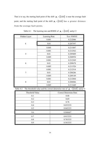
Here ,00 Z ,10  jr pj ,...,2,1 。
The MEWMA control chart will be out of control in the condition:
hZZT iZii i
 12
0h
The choice of the specific “in control” ARL (Average Run Length) is decided by
process personnel. If the parameters rrrrrr p  4321 , the statistics of
MEWMA can be written as:
  ,1-iZrIrXZ ii  ,...2,1i
 )}2/(])1(1[{ 2
rrr i
Zi
Here iZ is the covariance matrix of:
The MEWMA control chart can respond in a timely fashion when the process is out
control, especially the small shift, so producers can find the starting fault point of the
process quickly. Therefore, it would be a better choice when compared with other
multivariate control charts. The weakness of the MEWMA is restricted by the
correlation of data, and it cannot monitor biases or faults in time, so we can pair it with
the control line of the Hotelling 2
T chart and adjust the UCL and LCL. We also
combine the MEWMA with NN in hopes that it will have better differentiation ability
than combing the Hotelling 2
T control chart and NN.

32. 21
3.2.3 Weaknesses of the Multivariate Control Chart
Although multivariate control charts can track many quality characteristics, they
cannot monitor the starting fault point of the process. For instance, the Hotelling 2
T
can illustrate this weakness.
We assume the product has three quality characters and the process shift
obeys ),( 2
N . We then use SAS to simulate two times.
The first situation is that the observations do not shift; those points are inside the
control line ( 0 = (0, 0, 0),) and the process is in control. When the variable for the
quality characteristics P is 3, the sample group number m is 300, Sample size n is 5, and
the Hotelling 2
T control chart is as found in Figure 3-4. The UCL and LCL are the
control lines of the Hotelling 2
T control in the chart, and the computing method is as
follows:
UCL=T 1,,
2
1,,
1
)1)(1(



 pmmnppmmnp F
pmmn
nmp

LCL=0
Where, p=3, m=300, n=5,  =0.001,
We can compute:
UCL=T 133001500,3,001.0
2
133001500,3,001.0
133001500
)15)(1300(3



 F =16.34
LCL=0

33. 22
Figure 3-4 The shift 0 = (0, 0, 0) of Hotelling 2
T control chart
Our second situation assumes the process is in control from points 1 to 150, but
shifts after point 151. If the observations exceed the control line, the process is out of
control. That is to say 0 =0, u1 is the mean value of the shift and k is the average shift,
where k =0.5~3. The shift 1 = (0.5, 0, 0) represents the first quality characteristic
shift, where 1 = 0 +k x
 =0+0.5*1=0.5, and k=0.5, Figure 3-5 shows the case when
x
 =1. The UCL and LCL are the control lines of the Hotelling 2
T control chart
shown in that figure, and the computing methods are as follows:
UCL=T 1,,
2
1,,
1
)1)(1(



 pmmnppmmnp F
pmmn
nmp

LCL=0
We can compute:
0
2
4
6
8
10
12
14
16
18
1 21 41 61 81 101 121 141 161 181 201 221 241 261 281
UCL=16.34
T2
LCL=0

34. 23
UCL=T 133001500,3,001.0
2
133001500,3,001.0
133001500
)15)(1300(3



 F =16.34
LCL=0
Figure 3-5 The shift 1 =(0.5,0,0) of Hotelling 2
T control chart
We assume the system is out of control after the 151 st
data point. In Figure 3-4
each observation is in control because we assume 0 =(0,0,0), which is to say there is
not any point exceeding the control line. In Figure 3-5, we can see the point 195
exceeds the control line, the starting fault point of the process far from the initial point
151 that we assumed. If quality personnel desire to find the starting fault point of the
process and correct it, they must waste time and manpower. It is very costly to the
enterprise. Take 1 =(0.5,0,0) for an example. We assume every point wastes 100 U.S.
dollars and one day of work. When we inspect, the process must stop and find the point
in reverse step by step. In this example, it wastes 44 time points that is 44,000 U.S.
dollars and 44 days. It not only waste time and cost, but since it also cannot be
0
5
10
15
20
1 21 41 61 81 101 121 141 161 181 201 221 241 261 281
UCL=16.34
LCL=0
T2
Point 195

35. 24
delivered on time, it will lose many other orders. If we can monitor the 151 st
point,
the starting fault of the process, or find it earlier than with the multivariate control chart,
it will not waste as much time and cost. NN has the strengths of multivariate accuracy
and high quality data processing. If we combine a multivariate control chart and NN,
we hope to find the starting fault of the process earlier than before. Therefore, we
combine the Hotelling
2
T , the MEWMA control chart and NN to find the process’s
initial fault point.
3.3 Description of the Approach
It has been discovered that applications using multivariate control charts cannot
find out the starting fault point. Therefore we combine multivariate control charts with
NN to find the starting fault point quickly.
3.3.1 Binomial Distribution
Binomial distribution probability is application extensive and important. It can be
used to explain many results and be applied in many ways. Furthermore, during the
process of dealing with practical problems, we repeatedly use Bernoulli trials to solve
problems. We classify the outcomes as either “success” or “failure,” so binomial
distribution is also called binomial experience.
The criteria for this method are described as follows:

36. 25
(1) Must consist of n independence values and be tested using same course.
(2) Only success or failure are possible results of each test.
(3) The probability of a successful test is equal to Prob. for Prob. (0< Prob. <1 ), the
probability of succeeding each time is immobilized by the constants, and the failure
probability for each trial is all 1- Prob.=q.
(4) For specific N sized binomials the probability of complete mutual exclusion is less
than the probability of being totally independent. Thus the result of the tests will
not be affected by each other.
(5) The random parameter X is the number of times tested successfully,
X =0, 1, 2, …, n.
So we use X~b (n, Prob.) to express the incident for once in n tries, parameter Prob.
is present X times.
The random probability of X distributes the function：
nxobob
x
n
xf xnx
,...,1,0,.)Pr1(.Pr)( 





 
,
)!(!
!
xnx
n
x
n







=0 , other
Where n = Number of experimental iterations.
Prob. = Probability of Success
(1 - Prob. )= Probability of Failure
F (x) = Probability function of Binomial distribution density, where x is the
probability of success in n trials.
x= Number of times that n succeeds in time to get close to the binomial
distribution probability.

37. 26
(4) Transformations:
1. As n trends towards an almost infinitely great value and Prob. borders on 0, these
distributions of probability are similar to the Poisson distribution.
2. As n trends towards an almost infinitely great value, these distributions of probability
are similar to a Normal distribution.
In this research, we will simulate 1000 data points, and these 1000 data points will
accord with binomial distribution probability:
(1) Each observing value is a test, so 1000 points are 1000 tests, and the process of the
test each time is the same.
(2) There are only two kinds of results in the test each time (success or failure): If the
output value of NN is clicked for out of control for 1, we set up the output value of 0
mean failures, and probability is 1-Prob.; We click for in control for 0, we set up the
output value 1 mean success, and our probability is Prob..
(3) We assume that the probability of an out of control system for each observing value
is the successful probability, and the probability of succeeding in every observation
value is equal and independent.
These 1000 observations of probability function are:
nxobob
x
n
xf xnx
,...,1,0,.)Pr1(.Pr)( 





 
,
)!(!
!
xnx
n
x
n







, 0≦Prob.≦1
Where n = Number of experimental trials.
Prob. = Probability the NN model can successfully judge the system out of
control.

38. 27
(1 - Prob.) = Probability the NN model is unable to judge the system out of
control.
F (x) = Function showing that there are x out of control plots in n
observations.
3.3.2 Neural Networks (NN)
Neural networks refer to information processing systems that imitate the brain’s
neural system. It is a process-computing mode in the way of parallel distribution. The
technique of NN was developed by Rosenblatt when he proposed the perception model,
which was applied to the recognition of letters in business. NN has a great power of
classification, prediction and handling of data, so it is widely utilized. And it can learn
data that is considered the most complicated in the world.
Artificial Neural Networks (NN) are systems loosely modeled on an organism’s
brain. They consist of a computing-processing mode which is distributed in parallel.
Differing forms of neural development of network technology begin with Rosenblatt,
who applied it to aesthesia machines. It could be applied to commercial letters and
ascertain information. In recent years, science and technology have made progress, and
the applications of NN have increased. Classifications, treatment of materials and
prediction power have been extensively applied in many fields. Furthermore, it can
study repeated inputs, and it is thought these networks can handle the most complicated
information in the whole world. Because of the powerful abilities of classification,
information processing and forecasting, NN can be used extensively. They can learn

39. 28
from repeated data, and people from all over the world think of them when encountered
by complicated information.
NN have the ability of learning from input data and determining relationships
among data. During the training process, the learning rate is a very important
parameter. The learning rate will influence the rate of convergence. If a high
learning rate is chosen, the rate of convergence will be fast. The contrary is also true.
NN is a kind of computing system, and it utilizes the ability of living beings to organize,
as evidenced by its use of a large amount of artificial neurons. These are simple and
linked to each other to imitate the brain of an organism. Our studies are thus
biological simulations. After repeated practice and improvement, computer may one
day possess learning abilities similar to mankind’s own. And because NN has these
abilities, it can be used for such purposes as high-speed computation, memory, noise
filtering, and fault-tolerance etc. The basic construction is shown in Figure 3-6.
Input layer Hidden layer Output layer
Figure 3-6 The basic construction of NN
(1) Input layer
The neuron in the input layer is used as the introduction parameter in the

40. 29
behavioral neural network. It is mainly for receiving the input data and deciding
which to accept or otherwise deal with. It has no computing capability. The number of
input parameters depends on the state of the problem at hand. The data must first be
regularized, then undergo the linear transfer function.
(2) Hidden layer
The neuron in hidden layer lies between the input layer and the output layer. It is
used to deal with data sent from the input layer and transfer it to the output layer. It
uses the linear transfer function. The layer usually sees very little work because it only
increases complexity. This layer mainly displays the interaction among neural
processing units.
(3) Output layer
The output layer is used to display the output of NN. A network must first be
trained in order to maximize efficacy. One must make a NN learn repeatedly until all
inputs are entered into the NN and it can correspond to the output that we need. The
main purpose of training is to get output values near to target values, input values equal
to the output values. Before training, neural output value is in disorder. While training,
this is expressed as a training value. The errors of training values and actual values
will receive feedback and are corrected to the right value for each other (Connect
Weight), in order to reach the right value, until the network disappears. Increasing the
number training iterations will influence the goal value and the neuron outputs directly.
The errors become fewer and fewer. The number of training iterations depends on the
problem; it behaves according to a non-linear transfer function.

41. 30
3.4 Test Process and the Result
3.4.1 Constructing NN Model
We test the shift 1 = (0.5, 0, 0) from above, describe how to construct the NN
model, the process and method shown in Figure 3-7 :
700 training points RMSE restrains itself 500 points in control
300 testing points RMSE is the lowest 500 pts. out of control
Figure3-7 The process of constructing NN model
Step1: Constructing a suitable model
We simulate 1000 data points for the training sample, using the ratio 7:3 for the
training data to the testing data. If the training data is in control, the target value is 0；If
out of control, the target value is 1. In the testing data, the ratio of the data is 1:1, 500
points for each.
Step 2: Constructing a suitable model
Construct a
suitable model
Simulate the
process data to
test the model
Build
training
sample

42. 31
We combine the data exported from SAS and Q-net of NN software to construct
the model. Take 1 = (0.5,0 ,0) as an example:
（1） Layer number: 3 layers: input layer, hidden layer and output layer.
（2） Input layer: In the example there are three quality characteristics, so we use 3.
（3） Hidden layer: It is 2n±2, where n is the input variable, so we set 4, 5…8.
（4） Output layer: Conforming to uniform distribution value (0, 1). 0 is determined to
be correct, 1 is an error.
（5） Learning rate: We choose the values 0.001, 0.005 and 0.01.
The model needs to match three following criteria:
(a) The RMSE trend chart must restrain itself
The RMSE trend chart of the model must restrain itself to a constant value,
because it is training continuously as shown in Figure 3-8. If it does not hold to a
constant value, we cannot use the model.
Figure 3-8 RMSE trend chart

43. 32
(b) Finding the lowest RMSE value
After the RMSE is restrained, we want to find the lowest amount of test data for
the different hidden layers and learning rates, as shown in Table 3-1.
Table 3-1 RMSE for different numbers and learning rates
Hidden Layer
Learning
Rate
Test RMSE
0.001 0.295998
4 0.005 0.295834
0.01 0.296295
0.001 0.296108
5 0.005 0.295818
0.01 0.292627
0.001 0.296076
6 0.005 0.296042
0.01 0.296062
0.001 0.296035
7 0.005 0.296016
0.01 0.296813
0.001 0.296199
8 0.005 0.295895
0.01 0.296296
(c) The highest determined correct rate is the threshold value.
We can find the highest determined rate shown in Table 3-1. It is the p-value of the
binominal distribution, and it is also the needed threshold value. If the output is
smaller than the threshold value, we choose a value of 0. Correspondingly, if the
output is bigger than threshold value, we choose a value of 1. In this article, we set
threshold values from 0.1 to 0.9. If the output of the NN is smaller than the threshold

44. 33
value, it is under control. If the output is bigger than the threshold value, it is out of
control. We can observe that when the hidden layer is 5, the learning rate is 0.01,
RMSE is 0.292627 and the threshold value is 0.5. We have the highest correct
determined rate, at a value is 0.673333.
Table 3-2 The correct determine rate in every threshold value
Hidden Layer
Learning
Rate
Test RMSE
Threshold
Value
Correct
Determine Rate
0.1 0.533333
0.2 0.5833333
0.3 0.620000
0.4 0.6433333
5 0.01 0.292627 0.5 0.6733333
0.6 0.633333
0.7 0.596667
0.8 0.573333
0.9 0.520000
Step3：Simulate the process data to test the model
Using the model that we constructed from above, we can observe the condition
under different shifts. We use SAS to simulate another 1000 iterations, where the
points 1~500 are in control, and point 501 and up are out of control. The 501 st
point
is also the starting fault point for the process. We combine this model with NN to
determine the fault condition. In Table 3-3, the row for the 「Out of Control NN
Signal」is the condition determined by Q-net, where 1 the condition determined to be

45. 34
correct and 0 represents a determined error. The row listed as「Cumulative Number of
Out of Control NN Signals」is the cumulative number signal determined by NN, and the
「Sample Number in Reverse Order」is the fault point determined by SPC chart in
reverse. We use binomial distribution cumulative probability to assist us in
determining the starting fault of the process. In Table 3-3, the point 602 is the starting
fault point of the process as determined by SAS. When we seek a cumulative
probability as precise as 1 or 0.99, we can find the starting fault point at point 600. In
Table 3-3, we can know the NN out of control signal at point 598 and 599. We
speculate the process is disturbed by assignable reasons, or the value is found to be 0 by
NN. This would mean the cumulative probability of binomial distribution descent is
0.794448 and 0.52 at the point 599 and 598, respectively. When the cumulative
probability equals 0.98, we can find the starting fault point of the process at point 520.
When the cumulative probability equal 0.97, we can find the starting fault point of the
process at point 519. When the cumulative probability equals 0.96 and 0.95, we can
find the starting fault point of the process at point 510. In this way, we can find the
starting fault point even earlier when the cumulative probability is 0.9, speculated to be
number 506 as seen in Figure 3-3.
Keeping these results in mind, we can then observe the shift 1 =(0.5,0,0). In the
SPC chart monitor, the starting fault point is 602. If we combine the SPC chart with
NN, the starting fault point moves ahead to 506, when the cumulative binomial
distribution probability is 0.9. There is an improvement of 94 data points, which
works out to 9,400 U.S. dollars and 94 working days for the enterprise (according to the
previous calculation of US$100 waste/point and 1 day/point.). Therefore, it is an

46. 35
effective and useful tool to increase production efficiency in industrial applications.
Table 3-3 Example testing data
Sample NO.
Sample NO. in
Reverse Order
Out of Control
Signal of NN
Cumulative Number
of Out of Control
NN Signals
Cumulative
Binomial
Distribution
Probability
…
…
…
…
…
505
506
507
508
509
510
98
97
96
95
94
93
0
1
0
0
0
1
71
71
70
70
70
70
0.883666
0.911666
0.900520
0.925755
0.946084
0.961973
…
…
…
…
…517
518
519
520
86
85
84
83
1
0
0
1
65
64
64
64
0.962414
0.956410
0.970467
0.980712
…
…
…
…
…
596
597
598
599
600
601
602
7
6
5
4
3
2
1
1
1
0
0
1
1
1
5
4
3
3
3
2
1
0.724151
0.635535
0.525862
0.794448
1.000000
1.000000
1.000000

47. 36
Chapter 4 SIMULATION STUDIES AND
ANALYSIS
This chapter will discuss the simulation result of the Hotelling 2
T control chart
and MEWMA control chart in combination with a Neural Network (NN) to see whether
the system can determine the starting fault point in advance. In the NN section, we use
cumulative probability binomial distribution to determine the starting fault point of the
process.
4.1 Combination of Hotelling T2
Control Chart and
Neural Networks
In the Hotelling 2
T control chart section, the process shifts of the quality
characteristics obey the function ),( 2
N . In order to construct a NN model we
implement SAS programs to simulate 1000 data points where there are 700 points of
training data and 300 of the testing data. We can look for the smallest test RMSE in
each hidden layer and learning rate, and determine the highest correct rate in
correspondence with the threshold value. Then, we simulate another 1000 data points,
assuming numbers 1-500 are in control, and numbers 501-1000 undergo a shift. Here

48. 37
we use mean shift 1 = 0 +k x
 , where 0 is the mean when the process is in control,
that is 0 =0; 1 is the mean of the shift process; k is the shift, where k=0.5, 1, 3.
Using Hotelling 2
T control chart by itself, we record the starting fault point of
SPC, and the control lines are as follows:
UCL=T 1,,
2
1,,
1
)1)(1(



 pmmnppmmnp F
pmmn
nmp

LCL=0
After factoring in the NN, the threshold value can determine whether a point is
faulty or not, and use cumulative probability binomial distribution to reverse the starting
fault point. The probability of binomial distribution is the determining value rate.
For each different probability (Prob. =1, 0.99, 0.98, 0.90), we can compare the
corresponding starting fault point.
The experimental values use quality characteristics 3, 5, 8, 12 in the research, and
the simulation is run 100 times. The results are described in the following section.
4.1.1 p=3
We first explain the results from the small shift  0,0,11 μ . Using Table 4-1, we
can find the smallest RMSE for different hidden layers and learning rates. So the
hidden layer of  0,0,11 μ is 4, the learning rate is 0.01, and the RMSE is 0.207397.
According to this information, we find the biggest correct determinant rate of 0.846667,
and correspondingly, the threshold value is 0.6, which is shown in Table 4-2.
According to that table, we can find each of the threshold values and correctly

49. 38
determine rate in each shifts, which are shown in Table 4-3.
We use the SAS statistics program to run the simulation 100 times, and the results
are shown in Table 4-4. The starting fault point determined by SPC is 515.18,
approximate at the point 516. When SPC is combined with NN, the starting fault point
of the binomial distribution Prob. =1.00 is 503.36, approximate at point 504, advancing
by 12 points. The starting fault point of the binomial distribution Prob. =0.99 is
502.18, approximate the point 503, advanced by 13 points. So the starting fault point
of the binomial distribution Prob. =0.90 is 501.55, approximate the point 501, advanced
by 15 points. Thus when the quality characteristics p=3, and the shift is small, the
model can find the starting fault point earlier.
This is the same method used for the larger shift  0,0,21 μ and the all shift
 1,5.0,5.01 μ cases. Since we previously assumed the starting fault point is
number 501, we cannot find the starting point after combining NN. The results are all
the same from Prob.=0.99 to Prob.=0.90. As mentioned above, the determined effect
of SPC in combination with NN in the big shift and all shift cases do not appear when
the shift is small.
Therefore, when only using SPC chart in p=3, the starting fault point is far from
the assumed point 501. There is a small distance between the starting fault point found
by SPC in combination with NN and point 501, which we assumed for the study.
Different shifts will affect the time needed to determine the starting fault point. To
determine the time needed for a small shift  0,0,11 μ is more obvious than to find it
for the big shift  0,0,21 μ and the all shifts case  1,5.0,5.01 μ . In finding the
standard deviation, we determine the standard deviation in the big shift  0,0,21 μ to
be 0.66, and 17.53 for the small shift  0,0,11 μ , which are shown in Table 4-2. We
discover that the standard deviation in the small shift is greater than for the big shift.

50. 39
That is to say, the starting fault point of the shift  0,0,21 μ is near the average fault
point, and the starting fault point of the shift  0,0,11 μ has a greater distance
from the average fault points.
Table 4-1 The learning rate and RMSE of  0,0,11 μ and p=3
Hidden Layer Learning Rate Test RMSE
0.001 0.212046
4 0.01 0.207397
0.005 0.211087
5
0.001 0.212562
0.01 0.209409
0.005 0.208954
6
0.001 0.212369
0.01 0.209678
0.005 0.211526
7
0.001 0.212318
0.01 0.208286
0.005 0.209149
8
0.001 0.212884
0.01 0.208886
0.005 0.211649
Table 4-2 The threshold value and the correct determine rate of  0,0,11 μ and p=3
Threshold Value Correct Determine Rate
0.1 0.48
0.2 0.69
0.3 0.78
0.4 0.833333
0.5 0.843333
0.6 0.846667
0.7 0.813333
0.8 0.763333
0.9 0.563333

51. 40
Table 4-3 The models in different shifts of p=3
Models
Shifts
Hidden
Layer
Learning
Rate
Test RMSE
Threshold
Value
Correct
Determine Rate
 0,0,11 μ 4 0.01 0.207397 0.6 0.846667
 0,1,11 μ 6 0.01 0.128593 0.6 0.963333
 5.1,0,11 μ 5 0.01 0.103281 0.3 0.91
 1,5.0,5.01 μ 6 0.01 0.177842 0.5 0.913333
 0,0,21 μ 7 0.01 0.067276 0.5 0.99
Table 4-4 The different starting fault points of p=3 in every Prob.
Shifts
Prob.
 0,0,11 μ  0,1,11 μ  5.1,0,11 μ  1,5.0,5.01 μ  0,0,21 μ
SPC 515.58(17.53) 504.34 501.69(1.03) 507.55(6.68) 501.15(0.66)
Prob.=1.00 503.36(7.63) 501.78(3.69) 501(0) 503.20(4.92) 501.02(0.14)
Prob.=0.99 502.18(4.76) 501.78(2.14) 501(0) 503.20(4.92) 501.02(0.14)
Prob.=0.98 501.8(4.02) 501.78(2.14) 501(0) 503.20(4.92) 501.02(0.14)
Prob.=0.97 501.61(3.58) 501.78(2.14) 501(0) 503.20(4.92) 501.02(0.14)
Prob.=0.96 501.61(3.58) 501.78(2.14) 501(0) 503.20(4.92) 501.02(0.14)
Prob.=0.95 501.61(3.58) 501.78(2.14) 501(0) 503.20(4.92) 501.02(0.14)
Prob.=0.94 501.61(3.58) 501.78(2.14) 501(0) 503.20(4.92) 501.02(0.14)
Prob.=0.93 501.61(3.58) 501.78(2.14) 501(0) 503.20(4.92) 501.02(0.14)
Prob.=0.92 501.61(3.58) 501.78(2.14) 501(0) 503.20(4.92) 501.02(0.14)
Prob.=0.91 501.61(3.58) 501.78(2.14) 501(0) 503.20(4.92) 501.02(0.14)
Prob.=0.90 501.55(3.54) 501.78(2.14) 501(0) 503.20(4.92) 501.02(0.14)
4.1.2 p=5
We use the small shift  0,0,0,0,11 μ as an example. From the Table 4-5, we
know the threshold value is 0.3, and the correct determinant rate is 0.856667. Then,
the results are shown in Table 4-6 which has been run 100 times. The starting fault point
determined by SPC is approximate at the point 531. When SPC is combined with NN,

52. 41
the starting fault point of the binomial distribution Prob. =1.00 is approximate at the
point 519, advancing by 12 points. The starting fault point of the binomial distribution
Prob. =0.99 is approximate at the point 510, advanced by 21 points. So the starting
fault point of the binomial distribution Prob. =0.90 is approximate the point 504,
advanced by 17 points. Thus when the quality characteristics p=5, and the shift is
small, the model can find the starting fault point earlier.
This is the same method used for the larger shift  0,0,0,0,21 μ and the all
shift  5.0,5.0,5.0,5.0,5.01 μ cases. Since we previously assumed the starting fault
point is number 501, we cannot find the starting point after combining NN. The
results are all the same from Prob.=0.99 to Prob.=0.90. As mentioned above, the
determined effect of SPC in combination with NN in the big shift and all shift cases do
not appear when the shift is small.
Therefore, when only using SPC chart in p=5, the starting fault point is far from
the assumed point 501. There is a small distance between the starting fault point found
by SPC in combination with NN and point 501, which we assumed for the study.
Different shifts will affect the time needed to determine the starting fault point. To
determine the time needed for a small shift  0,0,0,0,11 μ is more obvious than to find
it for the big shift  0,0,0,0,21 μ and the all shifts case  5.0,5.0,5.0,5.0,5.01 μ .
In finding the standard deviation, we determine the standard deviation in the big shift
 0,0,0,0,21 μ to be 0.86, and 31.84 for the small shift  0,0,0,0,11 μ , which are
shown in Table 4-6. We discover that the standard deviation in the small shift is
greater than for the big shift. That is to say, the starting fault point of the shift
 0,0,0,0,21 μ is near the average fault point, and the starting fault point of the shift
 0,0,0,0,11 μ has a greater distance from the average fault points.

53. 42
Table 4-5 The models in different shifts of p=5
Models
Shifts
Hidden
Layer
Learning
Rate
Test RMSE
Threshold
Value
Correct
Determine
Rate
 0,0,0,0,11 μ 10 0.005 0.228178 0.3 0.856667
 0,0,0,1,11 μ 11 0.05 0.169625 0.4 0.906667
 0,0,0,0,21 μ 12 0.005 0.077257 0.5 0.986667
 5.0,5.0,5.0,5.0,5.01 μ 11 0.01 0.196828 0.4 0.906667
 0,0,1,5.0,5.01 μ 9 0.01 0.159630 0.5 0.933333
Table 4-6 The different starting fault points of p=5 in every Prob.
shifts
Prob.
 0,0,0,0,11 μ  0,0,0,1,11 μ  0,0,0,0,21 μ
SPC 530.10(31.84) 505.60(6.15) 501.52(0.86)
Prob.=1.00 518.98(25.54) 501.79(3.20) 501(0)
Prob.=0.99 509.35(14.28) 501.79(3.20) 501(0)
Prob.=0.98 507.73(13.37) 501.79(3.20) 501(0)
Prob.=0.97 506.39(11.72) 501.79(3.20) 501(0)
Prob.=0.96 506.17(11.64) 501.79(3.20) 501(0)
Prob.=0.95 505.79(11.03) 501.79(3.20) 501(0)
Prob.=0.94 504.75(9.46) 501.79(3.20) 501(0)
Prob.=0.93 504.29(8.56) 501.79(3.20) 501(0)
Prob.=0.92 504.01(8.40) 501.79(3.20) 501(0)
Prob.=0.91 503.29(6.06) 501.79(3.20) 501(0)
Prob.=0.90 503.27(6.06) 501.67(2.59) 501(0)

54. 43
Table 4-6 The different starting fault points of p=5 in every Prob. (Continued)
Shifts
Prob.
 5.0,5.0,5.0,5.0,5.01 μ  0,0,1,5.0,5.01 μ
SPC 518.39(19.05) 510.65(9.82)
Prob.=1.00 512.73(17.80) 505.96(7.62)
Prob.=0.99 512.73(17.80) 505.96(7.62)
Prob.=0.98 512.73(17.80) 505.96(7.62)
Prob.=0.97 511.98(16.50) 505.96(7.62)
Prob.=0.96 511.86(16.54) 505.96(7.62)
Prob.=0.95 511.86(16.54) 505.96(7.62)
Prob.=0.94 510.71(16.57) 505.96(7.62)
Prob.=0.93 510.88(14.43) 505.96(7.62)
Prob.=0.92 510.86(14.43) 505.96(7.62)
Prob.=0.91 510.75(14.46) 505.96(7.62)
Prob.=0.90 510.75(14.46) 505.96(7.62)
4.1.3 p=8
We use the small shift  0,0,0,0,0,0,0,11 μ as an example. From the Table 4-7,
we know the threshold value is 0.3, and the correct determinant rate is 0.506667. Then,
the results are shown in Table 4-8 which has been run 100 times. The starting fault
point determined by SPC is approximate at the point 540. When SPC is combined
with NN, the starting fault point of the binomial distribution Prob. =1.00 is approximate
at the point 502, advancing by 38 points. The starting fault point of the binomial
distribution Prob. =0.99 is approximate at the point 501, advanced by 39 points. So
the starting fault point of the binomial distribution Prob. =0.90 is approximate the point
501, advanced by 39 points. Thus when the quality characteristics p=8, and the shift is
small, the model can find the starting fault point earlier.
This is the same method used for the larger shift  0,0,0,0,0,0,0,21 μ and the all

55. 44
shift  0,0,5.0,5.0,1,1,5.1,5.11 μ cases. Since we previously assumed the starting
fault point is number 501, we cannot find the starting point after combining NN. The
results are all the same from Prob.=0.99 to Prob.=0.90. As mentioned above, the
determined effect of SPC in combination with NN in the big shift and all shift cases do
not appear when the shift is small.
Therefore, when only using SPC chart in p=8, the starting fault point is far from
the assumed point 501. There is a small distance between the starting fault point found
by SPC in combination with NN and point 501, which we assumed for the study.
Different shifts will affect the time needed to determine the starting fault point. To
determine the time needed for a small shift  0,0,0,0,0,0,0,11 μ is more obvious than
to find it for the big shift  0,0,0,0,0,0,0,21 μ and the all shifts
case  0,0,5.0,5.0,1,1,5.1,5.11 μ . In finding the standard deviation, we determine
the standard deviation in the big shift  0,0,0,0,0,0,0,21 μ to be 0.22, and 48.49 for
the small shift  0,0,0,0,0,0,0,11 μ , which are shown in Table 4-8. We discover that
the standard deviation in the small shift is greater than for the big shift. That is to say,
the starting fault point of the shift  0,0,0,0,0,0,0,21 μ is near the average fault point,
and the starting fault point of the shift  0,0,0,0,0,0,0,11 μ has a greater distance
from the average fault points.

56. 45
Table 4-7 The models in different shifts of p=8
Models
Shifts
Hidden
Layer
Learning
Rate
Test RMSE
Threshold
Value
Correct
Determine
Rate
 0,0,0,0,0,0,0,11 μ 18 0.001 0.414483 0.3 0.506667
 5.1,5.0,1,0,0,0,0,01 μ 16 0.01 0.100097 0.3 0.98
 0,5.0,0,5.0,0,1,0,11 μ 14 0.01 0.103893 0.4 0.976667
 0,0,5.0,5.0,1,1,5.1,5.11 μ 16 0.001 0.489151 0.5 0.496667
 0,0,0,0,0,0,0,21 μ 18 0.001 0.463957 0.9 0.55
Table 4-8 The different starting fault points of p=8 in every Prob.
Shifts
Prob.
 0,0,0,0,0,0,0,11 μ  5.1,5.0,1,0,0,0,0,01 μ  0,5.0,0,5.0,0,1,0,11 μ
SPC 539.97(48.49) 507.78(8.92) 505.30(5.05)
Prob.=1.00 501.2(1.04) 501.85(3.57) 501.44(1.77)
Prob.=0.99 501(0) 501.85(3.57) 501.44(1.77)
Prob.=0.98 501(0) 501.85(3.57) 501.44(1.77)
Prob.=0.97 501(0) 501.85(3.57) 501.44(1.77)
Prob.=0.96 501(0) 501.85(3.57) 501.44(1.77)
Prob.=0.95 501(0) 501.85(3.57) 501.44(1.77)
Prob.=0.94 501(0) 501.85(3.57) 501.44(1.77)
Prob.=0.93 501(0) 501.85(3.57) 501.44(1.77)
Prob.=0.92 501(0) 501.85(3.57) 501.44(1.77)
Prob.=0.91 501(0) 501.85(3.57) 501.44(1.77)
Prob.=0.90 501(0) 501.85(3.57) 501.44(1.77)
Table 4-8 The different starting fault points of p=8 in every Prob. (Continued)
Shifts
Prob.
 0,0,5.0,5.0,1,1,5.1,5.11 μ  0,0,0,0,0,0,0,21 μ
SPC 501.12(0.38) 501.05(0.22)
Prob.=1.00 501(0) 501(0)

57. 46
Prob.=0.99 501(0) 501(0)
Prob.=0.98 501(0) 501(0)
Prob.=0.97 501(0) 501(0)
Prob.=0.96 501(0) 501(0)
Prob.=0.95 501(0) 501(0)
Prob.=0.94 501(0) 501(0)
Prob.=0.93 501(0) 501(0)
Prob.=0.92 501(0) 501(0)
Prob.=0.91 501(0) 501(0)
Prob.=0.90 501(0) 501(0)
4.1.4 p=12
We use the small shift  0,0,0,0,0,0,0,0,0,0,0,11 μ as an example. From the
Table 4-9, we know the threshold value is 0.5, and the correct determinant rate is 0.87.
Then, the results are shown in Table 4-10 which has been run 100 times. The starting
fault point determined by SPC is approximate at the point 518. When SPC is
combined with NN, the starting fault point of the binomial distribution Prob. =1.00 is
approximate at the point 515, advancing by 3 points. The starting fault point of the
binomial distribution Prob. =0.99 is approximate at the point 515, advanced by 3 points.
So the starting fault point of the binomial distribution Prob. =0.90 is approximate the
point 511, advanced by 7 points. Thus when the quality characteristics p=12, and the
shift is small, the model can find the starting fault point earlier.
This is the same method used for the larger shift  0,0,0,0,0,0,0,0,0,0,0,21 μ and
the all shift  5.1,5.1,1,1,5.0,5.0,5.1,5.1,1,1,5.0,5.01 μ cases. Since we
previously assumed the starting fault point is number 501, we cannot find the starting
point after combining NN. The results are all the same from Prob.=0.99 to Prob.=0.90.
As mentioned above, the determined effect of SPC in combination with NN in the big

58. 47
shift and all shift cases do not appear when the shift is small.
Therefore, when only using SPC chart in p=12, the starting fault point is far from
the assumed point 501. There is a small distance between the starting fault point found
by SPC in combination with NN and point 501, which we assumed for the study.
Different shifts will affect the time needed to determine the starting fault point. To
determine the time needed for a small shift  0,0,0,0,0,0,0,0,0,0,0,11 μ is more
obvious than to find it for the big shift  0,0,0,0,0,0,0,0,0,0,0,21 μ and the all shifts
case  5.1,5.1,1,1,5.0,5.0,5.1,5.1,1,1,5.0,5.01 μ . In finding the standard
deviation, we determine the standard deviation in the big shift
 0,0,0,0,0,0,0,0,0,0,0,21 μ to be 0.28, and 34.65 for the small
shift  0,0,0,0,0,0,0,0,0,0,0,11 μ , which are shown in Table 4-10. We discover that the
standard deviation in the small shift is greater than for the big shift. That is to say, the
starting fault point of the shift  0,0,0,0,0,0,0,0,0,0,0,21 μ is near the average fault
point, and the starting fault point of the shift  0,0,0,0,0,0,0,0,0,0,0,11 μ has a greater
distance from the average fault points.
Table 4-9 The models in different shifts of p=12
Models
Shifts
Hidden
Layer
Learning
Rate
Test
RMSE
Threshold
Value
Correct
Determine
Rate
 0,0,0,0,0,0,0,0,0,0,0,11 μ 22 0.001 0.22038 0.5 0.87
 0,0,0,0,0,0,0,0,1,1,1,11 μ 24 0.01 0.063908 0.6 0.99
 0,0,0,0,0,0,5.1,5.1,1,1,5.0,5.01 μ 22 0.01 0.033089 0.5 0.996667
 5.1,5.1,1,1,5.0,5.0,5.1,5.1,1,1,5.0,5.01 μ 23 0.01 0.007785 0.5 1
 0,0,0,0,0,0,0,0,0,0,0,21 μ 26 0.01 0.067681 0.4 0.993333

59. 48
Table 4-10 The different starting fault points of p=12 in every Prob.
Shifts
Prob.
 0,0,0,0,0,0,0,0,0,0,0,11 μ  0,0,0,0,0,0,5.1,5.1,1,1,5.0,5.01 μ
SPC 517.40(34.65) 510.66(1.21)
Prob.=1.00 514.72(34.20) 501(0)
Prob.=0.99 514.72(34.20) 501(0)
Prob.=0.98 513.69(32.17) 501(0)
Prob.=0.97 513.69(32.17) 501(0)
Prob.=0.96 512.75(31.44) 501(0)
Prob.=0.95 511.73(31.20) 501(0)
Prob.=0.94 511.34(31.14) 501(0)
Prob.=0.93 510.68(30.28) 501(0)
Prob.=0.92 510.67(30.29) 501(0)
Prob.=0.91 510.67(30.29) 501(0)
Prob.=0.90 510.57(30.18) 501(0)
Table 4-10 The different starting fault points of p=8 in every Prob. (Continued)
Shifts
Prob.
 0,0,0,0,0,0,0,0,1,1,1,11 μ  5.1,5.1,1,1,5.0,5.0,5.1,5.1,1,1,5.0,5.01 μ
SPC 501.46(0.89) 501(0)
Prob.=1.00 501.04(0.24) 501(0)
Prob.=0.99 501.04(0.24) 501(0)
Prob.=0.98 501.04(0.24) 501(0)
Prob.=0.97 501.04(0.24) 501(0)
Prob.=0.96 501.04(0.24) 501(0)
Prob.=0.95 501.04(0.24) 501(0)
Prob.=0.94 501.04(0.24) 501(0)
Prob.=0.93 501.04(0.24) 501(0)
Prob.=0.92 501.04(0.24) 501(0)
Prob.=0.91 501.04(0.24) 501(0)
Prob.=0.90 501.04(0.24) 501(0)

60. 49
Table 4-10 The different starting fault points of p=8 in every Prob. (Continued)
Shifts
Prob.
 0,0,0,0,0,0,0,0,0,0,0,21 μ
SPC 501.06(0.28)
Prob.=1.00 501(0)
Prob.=0.99 501(0)
Prob.=0.98 501(0)
Prob.=0.97 501(0)
Prob.=0.96 501(0)
Prob.=0.95 501(0)
Prob.=0.94 501(0)
Prob.=0.93 501(0)
Prob.=0.92 501(0)
Prob.=0.91 501(0)
Prob.=0.90 501(0)
4.1.5 Analysis
At the number of quality characteristics p=3,5,8,12, we use small shift
 0,0,11 μ 、  0,0,0,0,11 μ 、  0,0,0,0,0,0,0,11 μ and  0,0,0,0,0,0,0,0,0,0,0,11 μ to
compare with one another, which are shown in Table 4-11. In the
shift  0,0,11 μ , the starting fault point determined by SPC is approximate at the point
516. When SPC is combined with NN, the starting fault point of the binomial
distribution Prob. =0.90 is approximate at the point 502, advancing by 14 points. In
the shift  0,0,0,0,11 μ , the starting fault point determined by SPC is approximate at the
point 531. When SPC is combined with NN, the starting fault point of the binomial
distribution Prob. =0.90 is approximate at the point 504, advancing by 27 points. In
the shift  0,0,0,0,0,0,0,11 μ , the starting fault point determined by SPC is approximate
at the point 540. When SPC is combined with NN, the starting fault point of the
binomial distribution Prob. =0.90 is approximate at the point 501, advancing by 39

61. 50
points. And in the shift  0,0,0,0,0,0,0,0,0,0,0,11 μ , the starting fault point determined
by SPC is approximate at the point 518. When SPC is combined with NN, the starting
fault point of the binomial distribution Prob. =0.90 is approximate at the point 511,
advancing by 7 points.
As mentioned above, we know that if we only use the SPC control chart, the
distance from the starting point to the 501st
point is very far. In the case in which
quality characteristics are different, we can find the result for all small shift cases. The
starting fault point will advance more if the number of quality characteristics is less than
the SPC control chart combined with NN, and it will fall close to the starting fault point
that we set. When we alter the quality characteristics, that no matter SPC control chart
or that combine with NN, both of the starting fault points will close on the assumed
value (point 501), only if the quality characteristics included bigger shifts or the case of
the shift in all quality characteristics. Because of this, we can find that, for situations
using big shifts and having plenty of quality characteristics, the decision of the starting
fault point in the Hotelling 2
T control chart is close to the real starting fault point.
And that means the Hotelling 2
T control chart has a greater capability regarding
situations having big shifts and plenty of quality characteristics.
Table 4-11 The small shift outcomes in different quality characteristics of Hotelling 2
T
Shifts
Prob.
 0,0,11 μ  0,0,0,0,11 μ  0,0,0,0,0,0,0,11 μ  0,0,0,0,0,0,0,0,0,0,0,11 μ
SPC 515.58 530.10 539.97 517.40
Prob.=0.90 501.55 503.27 501 510.57
Advance
Points
14 27 39 7

62. 51
4.2 Combination of MEWMA Control Chart and
Neural Networks
In MEWMA section, the steps are as same as Hotelling 2
T control chart. In
order to construct a NN model we implement SAS programs to simulate 1000 data
points where there are 700 points of training data and 300 of the testing data. In
determine the fault points section, we simulate another 1000 data points, assuming
numbers 1-500 are in control, and numbers 501-1000 undergo a shift. The control
lines referenced chosen by Montgomery(2005). We also use cumulative
probability binomial distribution to reverse the starting fault point. For each different
probability (Prob. =1, 0.99, 0.98, 0.90), we can compare the corresponding starting fault
point.
The experimental values use quality characteristics 2, 4, 6, 10 and
 =0.1,0.2,0.3,0.4 in the research, and the simulation is run 100 times. The results are
described in the following section.
4.2.1  =0.1
4.2.1.1 p=2
We use the small shift  0,11 μ as an example. From the Table 4-12, we know
the threshold value is 0.4, and the correct determinant rate is 0.65. Then, the results
are shown in Table 4-13 which has been run 100 times. The starting fault point
determined by SPC is approximate at the point 510. When SPC is combined with NN,

63. 52
the starting fault point of the binomial distribution Prob. =1.00 is approximate at the
point 506, advancing by 4 points. The starting fault point of the binomial distribution
Prob. =0.99 is approximate at the point 505, advanced by 5 points. So the starting
fault point of the binomial distribution Prob. =0.90 is approximate the point 503,
advanced by 7 points. Thus when the quality characteristics p=2, and the shift is small,
the model can find the starting fault point earlier.
This is the same method used for the larger shift  0,5.11 μ and the all shift
 5.0,5.11 μ cases. Since we previously assumed the starting fault point is
number 501, we cannot find the starting point after combining NN. The results are all
the same from Prob.=0.99 to Prob.=0.90. As mentioned above, the determined effect
of SPC in combination with NN in the big shift and all shift cases do not appear when
the shift is small.
Therefore, when only using SPC chart in p=12 and =0.1, the starting fault point is
far from the assumed point 501. There is a small distance between the starting fault
point found by SPC in combination with NN and point 501, which we assumed for the
study. Different shifts will affect the time needed to determine the starting fault point.
To determine the time needed for a small shift  0,11 μ is more obvious than to find it
for the big shift  0,5.11 μ and the all shifts case  5.0,5.11 μ . In finding the
standard deviation, we determine the standard deviation in the big shift  0,5.11 μ to
be 2.82, and 7.84 for the small shift  0,11 μ , which are shown in Table 4-10. We
discover that the standard deviation in the small shift is greater than for the big shift.
That is to say, the starting fault point of the shift  0,5.11 μ is near the average fault
point, and the starting fault point of the shift  0,11 μ has a greater distance from
the average fault points.

64. 53
Table 4-12 The models in different shifts of p=2 and =0.1
Models
Shifts
Hidden
Layer
Learning
Rate
Test
RMSE
Threshold
Value
Correct
Determine Rate
 0,11 μ 4 0.01 0.303674 0.4 0.65
 0,5.11 μ 2 0.001 0.303238 0.5 0.73
 5.0,5.11 μ 3 0.01 0.263039 0.4 0.806667
Table 4-13 The different starting fault points of p=2 and =0.1in every Prob.
Shifts
Prob.
 0,11 μ  0,5.11 μ  5.0,5.11 μ
SPC 509.75(7.84) 505.87(2.82) 505.44(2.17)
Prob.=1.00 505.55(3.08) 503.52(3.38) 502.85(2.52)
Prob.=0.99 504.92(3.10) 503.52(3.38) 502.85(2.52)
Prob.=0.98 504.61(4.92) 503.52(3.38) 502.85(2.52)
Prob.=0.97 504.16(4.53) 503.52(3.38) 502.85(2.52)
Prob.=0.96 503.82(4.53) 503.52(3.38) 502.85(2.52)
Prob.=0.95 503.57(4.44) 503.52(3.38) 502.85(2.52)
Prob.=0.94 503.36(4.36) 503.52(3.38) 502.85(2.52)
Prob.=0.93 503.2(4.33) 503.52(3.38) 502.85(2.52)
Prob.=0.92 503.06(4.25) 503.52(3.38) 502.85(2.52)
Prob.=0.91 502.96(4.19) 503.52(3.38) 502.85(2.52)
Prob.=0.90 502.96(4.19) 503.52(3.38) 502.85(2.52)
4.2.1.2 p=4
We use the small shift  0,0,0,5.01 μ as an example. From the Table 4-14, we
know the threshold value is 0.5, and the correct determinant rate is 0.633333. Then,
the results are shown in Table 4-13 which has been run 100 times. The starting fault
point determined by SPC is approximate at the point 548. When SPC is combined with
NN, the starting fault point of the binomial distribution Prob. =1.00 is approximate at
the point 539, advancing by 9 points. The starting fault point of the binomial

65. 54
distribution Prob. =0.99 is approximate at the point 539, advanced by 9 points. So the
starting fault point of the binomial distribution Prob. =0.90 is approximate the point 538,
advanced by 10 points. Thus when the quality characteristics p=4, and the shift is
small, the model can find the starting fault point earlier.
This is the same method used for the larger shift  0,0,1,5.01 μ and the all shift
 5.1,5.1,1,11 μ cases. Since we previously assumed the starting fault point is
number 501, we cannot find the starting point after combining NN. The results are all
the same from Prob.=0.99 to Prob.=0.90. As mentioned above, the determined effect
of SPC in combination with NN in the big shift and all shift cases do not appear when
the shift is small.
Therefore, when only using SPC chart in p=4 and =0.1, the starting fault point is
far from the assumed point 501. There is a small distance between the starting fault
point found by SPC in combination with NN and point 501, which we assumed for the
study. Different shifts will affect the time needed to determine the starting fault point.
To determine the time needed for a small shift  0,0,0,5.01 μ is more obvious than to
find it for the big shift  0,0,1,5.01 μ and the all shifts case  5.1,5.1,1,11 μ . In
finding the standard deviation, we determine the standard deviation in the big shift
 0,0,1,5.01 μ to be 6.82, and 24.98 for the small shift  0,0,0,5.01 μ , which are
shown in Table 4-15. We discover that the standard deviation in the small shift is
greater than for the big shift. That is to say, the starting fault point of the shift
 0,0,1,5.01 μ is near the average fault point, and the starting fault point of the shift
 0,0,0,5.01 μ has a greater distance from the average fault points.

66. 55
Table 4-14 The models in different shifts of p=4 and =0.1
Models
Shifts
Hidden
Layer
Learning
Rate
Test RMSE
Threshold
Value
Correct
Determine Rate
 0,0,0,5.01 μ 8 0.01 0.339682 0.5 0.633333
 5.1,5.1,1,11 μ 6 0.005 0.193433 0.5 0.89
 0,0,0,5.01 μ 7 0.001 0.308614 0.4 0.613333
Table 4-15 The different starting fault points of p=2 and  =0.1in every Prob.
Shifts
Prob.
 0,0,0,5.01 μ  5.1,5.1,1,11 μ  0,0,0,5.01 μ
SPC 547.17(24.98) 503.59(1.39) 510.93(6.82)
Prob.=1.00 538.37(22.54) 501.91(1.67) 509.43(6.84)
Prob.=0.99 538.37(22.56) 501.91(1.67) 509.12(6.84)
Prob.=0.98 538.37(22.52) 501.91(1.67) 508.75(6.93)
Prob.=0.97 538.32(22.66) 501.91(1.67) 508.63(6.94)
Prob.=0.96 538.32(22.67) 501.91(1.67) 508.36(7.03)
Prob.=0.95 538.32(22.85) 501.91(1.67) 508.18(7.07)
Prob.=0.94 538.17(22.85) 501.91(1.67) 507.8(7.23)
Prob.=0.93 538.07(22.85) 501.91(1.67) 507.75(7.25)
Prob.=0.92 537.91(22.96) 501.91(1.67) 507.55(7.34)
Prob.=0.91 537.87(22.96) 501.91(1.67) 506.62(7.05)
Prob.=0.90 537.83(22.96) 501.91(1.67) 506.62(7.05)
4.2.1.3 p=6
We use the small shift  0,0,0,0,5.0,11 μ as an example. From the Table
4-16, we know the threshold value is 0.5, and the correct determinant rate is 0.72.
Then, the results are shown in Table 4-17 which has been run 100 times. The starting
fault point determined by SPC is approximate at the point 510. When SPC is
combined with NN, the starting fault point of the binomial distribution Prob. =1.00 is

67. 56
approximate at the point 508, advancing by 2 points. The starting fault point of the
binomial distribution Prob. =0.99 is approximate at the point 508, advanced by 2 points.
So the starting fault point of the binomial distribution Prob. =0.90 is approximate the
point 507, advanced by 3 points. Thus when the quality characteristics p=6, and the
shift is small, the model can find the starting fault point earlier.
This is the same method used for the larger shift  5.1,5.0,0,0,5.0,5.11 μ and
the all shift  1,1,1,1,1,11 μ cases. Since we previously assumed the starting fault
point is number 501, we cannot find the starting point after combining NN. The
results are all the same from Prob.=0.99 to Prob.=0.90. As mentioned above, the
determined effect of SPC in combination with NN in the big shift and all shift cases do
not appear when the shift is small.
Therefore, when only using SPC chart in p=6 and =0.1, the starting fault point is
far from the assumed point 501. There is a small distance between the starting fault
point found by SPC in combination with NN and point 501, which we assumed for the
study. Different shifts will affect the time needed to determine the starting fault point.
To determine the time needed for a small shift  0,0,0,0,5.0,11 μ is more obvious
than to find it for the big shift  5.1,5.0,0,0,5.0,5.11 μ and the all shifts
case  1,1,1,1,1,11 μ . In finding the standard deviation, we determine the standard
deviation in the big shift  5.1,5.0,0,0,5.0,5.11 μ to be 1.79, and 5.85 for the small
shift  0,0,0,0,5.0,11 μ , which are shown in Table 4-17. We discover that the
standard deviation in the small shift is greater than for the big shift. That is to say, the
starting fault point of the shift  5.1,5.0,0,0,5.0,5.11 μ is near the average fault
point, and the starting fault point of the shift  0,0,0,0,5.0,11 μ has a greater
distance from the average fault points.

68. 57
Table 4-16 The models in different shifts of p=6 and =0.1
Models
Shifts
Hidden
Layer
Learning
Rate
Test RMSE
Threshold
Value
Correct
Determine Rate
 0,0,0,0,5.0,11 μ 12 0.001 0.308313 0.5 0.72
 5.1,5.0,0,0,5.0,5.11 μ 10 0.01 0.225269 0.5 0.863333
 1,1,1,1,1,11 μ 10 0.005 0.210540 0.5 0.86
Table 4-17 The different starting fault points of p=6 and  =0.1in every Prob.
Shifts
Prob.
 0,0,0,0,5.0,11 μ  5.1,5.0,0,0,5.0,5.11 μ  1,1,1,1,1,11 μ
SPC 509.94(5.85) 504.17(1.79) 503.97(1.43)
Prob.=1.00 507.51(6.01) 501.33(0.95) 501.67(1.32)
Prob.=0.99 507.25(5.94) 501.33(0.95) 501.67(1.32)
Prob.=0.98 507.01(5.95) 501.33(0.95) 501.67(1.32)
Prob.=0.97 506.94(5.99) 501.33(0.95) 501.67(1.32)
Prob.=0.96 506.92(5.98) 501.33(0.95) 501.67(1.32)
Prob.=0.95 506.89(5.99) 501.33(0.95) 501.63(1.28)
Prob.=0.94 506.82(5.93) 501.33(0.95) 501.63(1.28)
Prob.=0.93 506.82(5.93) 501.33(0.95) 501.63(1.28)
Prob.=0.92 506.71(5.92) 501.33(0.95) 501.63(1.28)
Prob.=0.91 506.6(5.90) 501.33(0.95) 501.63(1.28)
Prob.=0.90 506.6(5.90) 501.33(0.95) 501.63(1.28)
4.2.1.4 p=10
We use the small shift  0,0,0,0,0,0,0,0,0,11 μ as an example. From the Table
4-18, we know the threshold value is 0.5, and the correct determinant rate is 0.643333.
Then, the results are shown in Table 4-19 which has been run 100 times. The starting
fault point determined by SPC is approximate at the point 514. When SPC is combined
with NN, the starting fault point of the binomial distribution Prob. =1.00 is approximate

69. 58
at the point 512, advancing by 2 points. The starting fault point of the binomial
distribution Prob. =0.99 is approximate at the point 512, advance by 2 points. So the
starting fault point of the binomial distribution Prob. =0.90 is approximate the point 508,
advanced by 6 points. Thus when the quality characteristics p=10, and the shift is
small, the model can find the starting fault point earlier.
This is the same method used for the larger shift
 0,5.1,0,1,0,5.0,0,1,0,5.01 μ and the all shifts
 5.1,5.0,1,1,5.1,5.1,5.0,5.0,1,11 μ cases. Since we previously assumed the
starting fault point is number 501, we cannot find the starting point after combining NN.
The results are all the same from Prob.=0.99 to Prob.=0.90. As mentioned above, the
determined effect of SPC in combination with NN in the big shift and all shift cases do
not appear when the shift is small.
Therefore, when only using SPC chart in p=10 and =0.1, the starting fault point is
far from the assumed point 501. There is a small distance between the starting fault
point found by SPC in combination with NN and point 501, which we assumed for the
study. Different shifts will affect the time needed to determine the starting fault point.
To determine the time needed for a small shift  0,0,0,0,0,0,0,0,0,11 μ is more
obvious than to find it for the big shift  0,5.1,0,1,0,5.0,0,1,0,5.01 μ and the all shifts
case  5.1,5.0,1,1,5.1,5.1,5.0,5.0,1,11 μ . In finding the standard deviation, we
determine the standard deviation in the big shift  0,5.1,0,1,0,5.0,0,1,0,5.01 μ to be
1.94, and 7.95 for the small shift  0,0,0,0,0,0,0,0,0,11 μ , which are shown in Table
4-19. We discover that the standard deviation in the small shift is greater than for the
big shift. That is to say, the starting fault point of the shift
 0,5.1,0,1,0,5.0,0,1,0,5.01 μ is near the average fault point, and the starting fault
point of the shift  0,0,0,0,0,0,0,0,0,11 μ has a greater distance from the

70. 59
average fault points.
Table 4-18 The models in different shifts of p=10 and =0.1
Models
Shifts
Hidden
Layer
Learning
Rate
Test
RMSE
Threshold
Value
Correct
Determine
Rate
 0,0,0,0,0,0,0,0,0,11 μ 20 0.001 0.300874 0.5 0.643333
 0,5.1,0,1,0,5.0,0,1,0,5.01 μ 21 0.01 0.203594 0.5 0.883333
 5.1,5.0,1,1,5.1,5.1,5.0,5.0,1,11 μ 18 0.005 0.119306 0.7 0.973333
Table 4-19 The different starting fault points of p=10 and  =0.1 in every Prob.
Shifts
Prob.
 0,0,0,0,0,0,0,0,0,11 μ  0,5.1,0,1,0,5.0,0,1,0,5.01 μ
SPC 513.59(7.95) 504.86(1.94)
Prob.=1.00 511.36(8.52) 502.85(2.20)
Prob.=0.99 511.21(8.62) 502.85(2.20)
Prob.=0.98 510.53(8.63) 502.85(2.20)
Prob.=0.97 509.83(8.47) 502.85(2.20)
Prob.=0.96 509.71(8.53) 502.85(2.20)
Prob.=0.95 509.29(8.32) 502.85(2.20)
Prob.=0.94 508.74(8.31) 502.85(2.20)
Prob.=0.93 508.73(8.32) 502.85(2.20)
Prob.=0.92 507.83(8.03) 502.85(2.20)
Prob.=0.91 507.79(8.02) 502.85(2.20)
Prob.=0.90 507.79(8.02) 502.85(2.20)

71. 60
Table 4-19 The different starting fault points of p=10 and  =0.1 in every Prob.
(Continued)
Shifts
Prob.
 5.1,5.0,1,1,5.1,5.1,5.0,5.0,1,11 μ
SPC 502.7(0.82)
Prob.=1.00 501.02(0.14)
Prob.=0.99 501.02(0.14)
Prob.=0.98 501.02(0.14)
Prob.=0.97 501.02(0.14)
Prob.=0.96 501.02(0.14)
Prob.=0.95 501.02(0.14)
Prob.=0.94 501.02(0.14)
Prob.=0.93 501.02(0.14)
Prob.=0.92 501.02(0.14)
Prob.=0.91 501.02(0.14)
Prob.=0.90 501.02(0.14)
4.2.2  =0.2
4.2.2.1 p=2
We use the small shift  0,11 μ as an example. From the Table 4-20, we know
the threshold value is 0.5, and the correct determinant rate is 0.72. Then, the results
are shown in Table 4-21 which has been run 100 times. The starting fault point
determined by SPC is approximate at the point 510. When SPC is combined with NN,
the starting fault point of the binomial distribution Prob. =1.00 is approximate at the
point 507, advancing by 3 points. The starting fault point of the binomial distribution
Prob. =0.99 is approximate at the point 507, advance by 3 points. So the starting fault
point of the binomial distribution Prob. =0.90 is approximate the point 506, advanced

72. 61
by 4 points. Thus when the quality characteristics p=2, and the shift is small, the
model can find the starting fault point earlier.
This is the same method used for the larger shift  0,5.11 μ and the all
shifts  5.0,5.11 μ cases. Since we previously assumed the starting fault point is
number 501, we cannot find the starting point after combining NN. The results are all
the same from Prob.=0.99 to Prob.=0.90. As mentioned above, the determined effect
of SPC in combination with NN in the big shift and all shift cases do not appear when
the shift is small.
Therefore, when only using SPC chart in p=2 and  =0.2, the starting fault point is
far from the assumed point 501. There is a small distance between the starting fault
point found by SPC in combination with NN and point 501, which we assumed for the
study. Different shifts will affect the time needed to determine the starting fault point.
To determine the time needed for a small shift  0,11 μ is more obvious than to find it
for the big shift  0,5.11 μ and the all shifts case  5.0,5.11 μ . In finding the
standard deviation, we determine the standard deviation in the big shift  0,5.11 μ to
be 2.52, and 5.51 for the small shift  0,11 μ , which are shown in Table 4-21. We
discover that the standard deviation in the small shift is greater than for the big shift.
That is to say, the starting fault point of the shift  0,5.11 μ is near the average fault
point, and the starting fault point of the shift  0,11 μ has a greater distance from
the average fault points.

73. 62
Table 4-20 The models in different shifts of p=2 and =0.2
Models
Shifts
Hidden
Layer
Learning
Rate
Test RMSE
Threshold
Value
Correct Determine
Rate
 0,11 μ 5 0.001 0.301791 0.5 0.72
 0,5.11 μ 6 0.01 0.259719 0.5 0.82
 5.0,5.11 μ 4 0.01 0.247213 0.5 0.766667
Table 4-21 The different starting fault points of p=2 and  =0.2 in every Prob.
4.2.2.2 p=4
We use the small shift  0,0,0,5.01 μ as an example. From the Table 4-22, we
know the threshold value is 0.3, and the correct determinant rate is 0.556667. Then,
the results are shown in Table 4-23 which has been run 100 times. The starting fault
point determined by SPC is approximate at the point 541. When SPC is combined with
NN, the starting fault point of the binomial distribution Prob. =1.00 is approximate at
the point 503, advancing by 38 points. The starting fault point of the binomial
Shifts
Prob.
 0,11 μ  0,5.11 μ  5.0,5.11 μ
SPC 509.44(5.51) 505.11(2.52) 503.16(2.16)
Prob.=1.00 506.78(5.07) 503.38(2.58) 501.14(0.58)
Prob.=0.99 506.78(5.07) 503.38(2.58) 501.14(0.58)
Prob.=0.98 506.64(4.94) 503.38(2.58) 501.14(0.58)
Prob.=0.97 506.53(4.93) 503.38(2.58) 501.14(0.58)
Prob.=0.96 506.53(4.93) 503.38(2.58) 501.14(0.58)
Prob.=0.95 506.43(4.73) 503.38(2.58) 501.14(0.58)
Prob.=0.94 506.07(4.47) 503.38(2.58) 501.14(0.58)
Prob.=0.93 505.91(4.41) 503.38(2.58) 501.14(0.58)
Prob.=0.92 505.58(3.90) 503.38(2.58) 501.14(0.58)
Prob.=0.91 505.15(3.43) 503.38(2.58) 501.14(0.58)
Prob.=0.90 505.07(3.42) 503.38(2.58) 501.14(0.58)

74. 63
distribution Prob. =0.99 is approximate at the point 503, advance by 38 points. So the
starting fault point of the binomial distribution Prob. =0.90 is approximate the point 501,
advanced by 40 points. Thus when the quality characteristics p=4, and the shift is
small, the model can find the starting fault point earlier.
This is the same method used for the larger shift  0,0,1,5.01 μ and the all
shift  5.1,5.1,1,11 μ cases. Since we previously assumed the starting fault point is
number 501, we cannot find the starting point after combining NN. The results are all
the same from P=0.99 to P=0.90. As mentioned above, the determined effect of SPC
in combination with NN in the big shift and all shift cases do not appear when the shift
is small.
Therefore, when only using SPC chart in p=4 and =0.2, the starting fault point is
far from the assumed point 501. There is a small distance between the starting fault
point found by SPC in combination with NN and point 501, which we assumed for the
study. Different shifts will affect the time needed to determine the starting fault point.
To determine the time needed for a small shift  0,0,0,5.01 μ is more obvious than to
find it for the big shift  0,0,1,5.01 μ and the all shifts case  5.1,5.1,1,11 μ . In
finding the standard deviation, we determine the standard deviation in the big shift
 0,0,1,5.01 μ to be 7.44, and 29.86 for the small shift  0,0,0,5.01 μ , which are
shown in Table 4-23. We discover that the standard deviation in the small shift is
greater than for the big shift. That is to say, the starting fault point of the shift
 0,0,1,5.01 μ is near the average fault point, and the starting fault point of the shift
 0,0,0,5.01 μ has a greater distance from the average fault points.

75. 64
Table 4-22 The models in different shifts of p=4 and =0.2
Models
Shifts
Hidden
Layer
Learning
Rate
Test RMSE
Threshold
Value
Correct Determine
Rate
 0,0,0,5.01 μ 6 0.005 0.349801 0.3 0.556667
 5.1,5.1,1,11 μ 6 0.01 0.188463 0.3 0.893333
 0,0,1,5.01 μ 7 0.001 0.27983 0.4 0.793333
Table 4-23 The different starting fault points of p=4 and  =0.2in every Prob.
Shifts
Prob.
 0,0,0,5.01 μ  5.1,5.1,1,11 μ  0,0,1,5.01 μ
SPC 540.46(29.86) 503.04(1.07) 510.88(7.44)
Prob.=1.00 502.48(4.70) 501.29(0.88) 509.52(7.63)
Prob.=0.99 501(0) 501.29(0.88) 509.52(7.63)
Prob.=0.98 501(0) 501.29(0.88) 509.52(7.63)
Prob.=0.97 501(0) 501.29(0.88) 509.52(7.63)
Prob.=0.96 501(0) 501.29(0.88) 509.52(7.63)
Prob.=0.95 501(0) 501.29(0.88) 509.52(7.63)
Prob.=0.94 501(0) 501.29(0.88) 509.52(7.63)
Prob.=0.93 501(0) 501.29(0.88) 509.52(7.63)
Prob.=0.92 501(0) 501.29(0.88) 509.52(7.63)
Prob.=0.91 501(0) 501.29(0.88) 509.52(7.63)
Prob.=0.90 501(0) 501.29(0.88) 509.52(7.63)
4.2.2.3 p=6
We use the small shift  0,0,0,0,5.0,11 μ as an example. From the Table
4-24, we know the threshold value is 0.5, and the correct determinant rate is 0.72.
Then, the results are shown in Table 4-25 which has been run 100 times. The starting
fault point determined by SPC is approximate at the point 512. When SPC is combined
with NN, the starting fault point of the binomial distribution Prob. =1.00 is approximate
at the point 509, advancing by 3 points. The starting fault point of the binomial

76. 65
distribution Prob. =0.99 is approximate at the point 509, advanced by 3 points. So the
starting fault point of the binomial distribution Prob. =0.90 is approximate the point 506,
advanced by 6 points. Thus when the quality characteristics p=6, and the shift is small,
the model can find the starting fault point earlier.
This is the same method used for the larger shift  5.1,5.0,0,0,5.0,5.11 μ and
the all shift  1,1,1,1,1,11 μ cases. Since we previously assumed the starting fault
point is number 501, we cannot find the starting point after combining NN. The
results are all the same from P=0.99 to P=0.90. As mentioned above, the determined
effect of SPC in combination with NN in the big shift and all shift cases do not appear
when the shift is small.
Therefore, when only using SPC chart in p=6 and =0.2, the starting fault point is
far from the assumed point 501. There is a small distance between the starting fault
point found by SPC in combination with NN and point 501, which we assumed for the
study. Different shifts will affect the time needed to determine the starting fault point.
To determine the time needed for a small shift  0,0,0,0,5.0,11 μ is more obvious
than to find it for the big shift  5.1,5.0,0,0,5.0,5.11 μ and the all shifts
case  1,1,1,1,1,11 μ . In finding the standard deviation, we determine the standard
deviation in the big shift  5.1,5.0,0,0,5.0,5.11 μ to be 1.53, and 7.23 for the small
shift  0,0,0,0,5.0,11 μ , which are shown in Table 4-25. We discover that the
standard deviation in the small shift is greater than for the big shift. That is to say, the
starting fault point of the shift  5.1,5.0,0,0,5.0,5.11 μ is near the average fault
point, and the starting fault point of the shift  0,0,0,0,5.0,11 μ has a greater
distance from the average fault points.

77. 66
Table 4-24 The models in different shifts of p=6 and =0.2.
Models
Shifts
Hidden
Layer
Learning
Rate
Test RMSE
Threshold
Value
Correct
Determine Rate
 0,0,0,0,5.0,11 μ 14 0.001 0.301731 0.5 0.64
 5.1,5.0,0,0,5.0,5.11 μ 13 0.01 0.223579 0.4 0.836667
 1,1,1,1,1,11 μ 13 0.005 0.206174 0.5 0.86
Table 4-25 The different starting fault points of p=6 and  =0.2 in every Prob.
Shifts
Prob.
 0,0,0,0,5.0,11 μ  5.1,5.0,0,0,5.0,5.11 μ  1,1,1,1,1,11 μ
SPC 511.38(7.23) 503.75(1.53) 503.41(1.16)
Prob.=1.00 508.64(7.34) 501.32(1.08) 501.88(1.36)
Prob.=0.99 508.09(6.98) 501.32(1.08) 501.88(1.36)
Prob.=0.98 507.77(7.12) 501.32(1.08) 501.88(1.36)
Prob.=0.97 507.53(7.08) 501.32(1.08) 501.88(1.36)
Prob.=0.96 507.24(7.09) 501.32(1.08) 501.88(1.36)
Prob.=0.95 507(6.95) 501.32(1.08) 501.88(1.36)
Prob.=0.94 506.65(6.70) 501.32(1.08) 501.88(1.36)
Prob.=0.93 506.34(6.61) 501.32(1.08) 501.88(1.36)
Prob.=0.92 506.03(6.57) 501.32(1.08) 501.88(1.36)
Prob.=0.91 505.99(6.59) 501.32(1.08) 501.88(1.36)
Prob.=0.90 505.97(6.57) 501.32(1.08) 501.88(1.36)
4.2.2.4 p=10
We use the small shift  0,0,0,0,0,0,0,0,0,11 μ as an example. We use the small
shift  0,0,0,0,0,0,0,0,0,11 μ as an example. From the Table 4-26, we know the
threshold value is 0.5, and the correct determinant rate is 0.643333. Then, the results
are shown in Table 4-27 which has been run 100 times. The starting fault point
determined by SPC is approximate at the point 514. When SPC is combined with NN,
the starting fault point of the binomial distribution Prob. =1.00 is approximate at the
point 512, advancing by 2 points. The starting fault point of the binomial distribution

78. 67
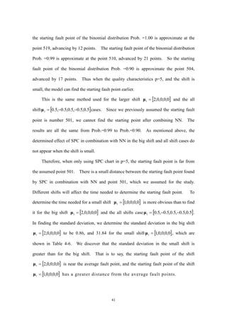
Prob. =0.99 is approximate at the point 511, advanced by 3 points. So the starting fault
point of the binomial distribution Prob. =0.90 is approximate the point 507, advanced
by 7 points. Thus when the quality characteristics p=10, and the shift is small, the
model can find the starting fault point earlier.
This is the same method used for the larger shift ]0,5.1,0,1,0,5.0,0,1,0,5.0[1 μ and the
all shifts  5.1,5.0,1,1,5.1,5.1,5.0,5.0,1,11 μ cases. Since we previously assumed the
starting fault point is number 501, we cannot find the starting point after combining NN.
The results are all the same from Prob.=0.99 to Prob.=0.90. As mentioned above, the
determined effect of SPC in combination with NN in the big shift and all shift cases do
not appear when the shift is small.
Therefore, when only using SPC chart in p=10 and =0.2, the starting fault point is
far from the assumed point 501. There is a small distance between the starting fault
point found by SPC in combination with NN and point 501, which we assumed for the
study. Different shifts will affect the time needed to determine the starting fault point.
To determine the time needed for a small shift  0,0,0,0,0,0,0,0,0,11 μ is more obvious
than to find it for the big shift ]0,5.1,0,1,0,5.0,0,1,0,5.0[1 μ and the all shifts
case  5.1,5.0,1,1,5.1,5.1,5.0,5.0,1,11 μ . In finding the standard deviation, we determine the
standard deviation in the big shift ]0,5.1,0,1,0,5.0,0,1,0,5.0[1 μ to be 2.06, and 9.23 for
the small shift  0,0,0,0,0,0,0,0,0,11 μ , which are shown in Table 4-27. We discover
that the standard deviation in the small shift is greater than for the big shift. That is to
say, the starting fault point of the shift ]0,5.1,0,1,0,5.0,0,1,0,5.0[1 μ is near the average
fault point, and the starting fault point of the shift  0,0,0,0,0,0,0,0,0,11 μ has a
greater distance from the average fault points.

79. 68
Table 4-26 The models in different shifts of p=10 and =0.2.
Models
Shifts
Hidden
Layer
Learning
Rate
Test RMSE
Threshold
Value
Correct
Determine
Rate
 0,0,0,0,0,0,0,0,0,11 μ 21 0.005 0.318932 0.5 0.61
]0,5.1,0,1,0,5.0,0,1,0,5.0[1 μ 21 0.005 0.216299 0.4 0.86
 5.1,5.0,1,1,5.1,5.1,5.0,5.0,1,11 μ 20 0.005 0.140889 0.3 0.953333
Table 4-27 The different starting fault points of p=10 and  =0.2in every Prob.
Shifts
Prob.
 0,0,0,0,0,0,0,0,0,11 μ ]0,5.1,0,1,0,5.0,0,1,0,5.0[1 μ
SPC 513.33(9.23) 504.54(2.06)
Prob.=1.00 511.09(9.25) 502.04(2.23)
Prob.=0.99 510.41(8.94) 502.04(2.23)
Prob.=0.98 509.94(9.21) 502.04(2.23)
Prob.=0.97 509.44(8.77) 502.04(2.23)
Prob.=0.96 508.59(8.69) 502.04(2.23)
Prob.=0.95 508.27(8.59) 502.04(2.23)
Prob.=0.94 507.69(8.36) 502.04(2.23)
Prob.=0.93 507.45(8.24) 502.04(2.23)
Prob.=0.92 506.88(7.90) 502.04(2.23)
Prob.=0.91 506.43(7.65) 502.04(2.23)
Prob.=0.90 506.31(7.67) 502.04(2.23)

80. 69
Table 4-27 The different starting fault points of p=10 and  =0.2 in every Prob.
(Continued)
Shifts
Prob.
 5.1,5.0,1,1,5.1,5.1,5.0,5.0,1,11 μ
SPC 502.47(0.86)
Prob.=1.00 501.06(0.34)
Prob.=0.99 501.06(0.34)
Prob.=0.98 501.06(0.34)
Prob.=0.97 501.06(0.34)
Prob.=0.96 501.06(0.34)
Prob.=0.95 501.06(0.34)
Prob.=0.94 501.06(0.34)
Prob.=0.93 501.06(0.34)
Prob.=0.92 501.06(0.34)
Prob.=0.91 501.06(0.34)
Prob.=0.90 501.06(0.34)
4.2.3  =0.3
4.2.3.1 p=2
We use the small shift  0,11 μ as an example. From the Table 4-28, we know
the threshold value is 0.4, and the correct determinant rate is 0.643333. Then, the
results are shown in Table 4-29 which has been run 100 times. The starting fault point
determined by SPC is approximate at the point 511. When SPC is combined with NN,
the starting fault point of the binomial distribution Prob. =1.00 is approximate at the
point 507, advancing by 4 points. The starting fault point of the binomial distribution
Prob. =0.99 is approximate at the point 505, advance by 6 points. So the starting fault
point of the binomial distribution Prob. =0.90 is approximate the point 502, advanced
by 9 points. Thus when the quality characteristics p=2, and the shift is small, the

81. 70
model can find the starting fault point earlier.
This is the same method used for the larger shift  0,5.11 μ and the all
shift  5.0,5.11 μ cases. Since we previously assumed the starting fault point is
number 501, we cannot find the starting point after combining NN. The results are all
the same from Prob.=0.99 to Prob.=0.90. As mentioned above, the determined effect
of SPC in combination with NN in the big shift and all shift cases do not appear when
the shift is small.
Therefore, when only using SPC chart in p=2 and  =0.3, the starting fault point is
far from the assumed point 501. There is a small distance between the starting fault
point found by SPC in combination with NN and point 501, which we assumed for the
study. Different shifts will affect the time needed to determine the starting fault point.
To determine the time needed for a small shift  0,11 μ is more obvious than to find it
for the big shift  0,5.11 μ and the all shifts case  5.0,5.11 μ . In finding the
standard deviation, we determine the standard deviation in the big shift  0,5.11 μ to
be 3.02, and 9.32 for the small shift  0,11 μ , which are shown in Table 4-29. We
discover that the standard deviation in the small shift is greater than for the big shift.
That is to say, the starting fault point of the shift  0,5.11 μ is near the average fault
point, and the starting fault point of the shift  0,11 μ has a greater distance from
the average fault points.

82. 71
Table 4-28 The models in different shifts of p=2 and =0.3.
Models
Shifts
Hidden
Layer
Learning
Rate
Test RMSE Threshold Value
Correct
Determine Rate
 0,11 μ 3 0.005 0.307951 0.4 0.643333
 0,5.11 μ 2 0.005 0.264613 0.5 0.793333
 5.0,5.11 μ 4 0.01 0.247213 0.5 0.82
Table 4-29 The different starting fault points of p=2 and  =0.3 in every Prob.
4.2.3.2 p=4
We use the small shift  0,0,0,5.01 μ as an example. From the Table 4-30, we
know the threshold value is 0.7, and the correct determinant rate is 0.506667. Then,
the results are shown in Table 4-31 which has been run 100 times. The starting fault
point determined by SPC is approximate at the point 561. When SPC is combined with
NN, the starting fault point of the binomial distribution Prob. =1.00 is approximate at
the point 555, advancing by 6 points. The starting fault point of the binomial
distribution Prob. =0.99 is approximate at the point 555, advanced by 6 points. So the
Shifts
Prob.
 0,11 μ  0,5.11 μ  5.0,5.11 μ
SPC 510.71(9.32) 504.95(3.02) 504.44(1.13)
Prob.=1.00 506.54(9.07) 503.1(3.00) 501.23(0.43)
Prob.=0.99 504.77(5.60) 503.1(3.00) 501.23(0.43)
Prob.=0.98 503.32(3.71) 503.1(3.00) 501.23(0.43)
Prob.=0.97 502.63(2.93) 503.1(3.00) 501.23(0.43)
Prob.=0.96 502.53(2.87) 503.1(3.00) 501.23(0.43)
Prob.=0.95 502.25(2.65) 503.1(3.00) 501.23(0.43)
Prob.=0.94 502.19(2.65) 503.1(3.00) 501.23(0.43)
Prob.=0.93 502.11(2.44) 503.1(3.00) 501.23(0.43)
Prob.=0.92 501.91(2.28) 503.1(3.00) 501.23(0.43)
Prob.=0.91 501.84(2.22) 503.1(3.00) 501.23(0.43)
Prob.=0.90 501.83(2.21) 503.1(3.00) 501.23(0.43)

83. 72
starting fault point of the binomial distribution Prob. =0.90 is approximate the point 554,
advanced by 7 points. Thus when the quality characteristics p=4, and the shift is small,
the model can find the starting fault point earlier.
This is the same method used for the larger shift  0,0,1,5.01 μ and the all
shift  5.1,5.1,1,11 μ cases. Since we previously assumed the starting fault point is
number 501, we cannot find the starting point after combining NN. The results are all
the same from Prob.=0.99 to Prob.=0.90. As mentioned above, the determined effect
of SPC in combination with NN in the big shift and all shift cases do not appear when
the shift is small.
Therefore, when only using SPC chart in p=4 and =0.3, the starting fault point is
far from the assumed point 501. There is a small distance between the starting fault
point found by SPC in combination with NN and the point 501, which we assumed for
the study. Different shifts will affect the time needed to determine the starting fault
point. To determine the time needed for a small shift  0,0,0,5.01 μ is more
obvious than to find it for the big shift  0,0,1,5.01 μ and the all shifts
case  5.1,5.1,1,11 μ . In finding the standard deviation, we determine the standard
deviation in the big shift  0,0,1,5.01 μ to be 7.86, and 30.53 for the small
shift  0,0,0,5.01 μ , which are shown in Table 4-31. We discover that the standard
deviation in the small shift is greater than for the big shift. That is to say, the starting
fault point of the shift  0,0,1,5.01 μ is near the average fault point, and the starting
fault point of the shift  0,0,0,5.01 μ has a greater distance from the average
fault points.

84. 73
Table 4-30 The models in different shifts of p=4 and =0.3
Models
Shifts
Hidden
Layer
Learning
Rate
Test RMSE
Threshold
Value
Correct
Determine Rate
 0,0,0,5.01 μ 10 0.001 0.337133 0.7 0.506667
 5.1,5.1,1,11 μ 6 0.005 0.201342 0.6 0.906667
 0,0,1,5.01 μ 9 0.001 0.305485 0.3 0.63
Table 4-31 The different starting fault points of p=4 and  =0.3in every Prob.
Shifts
Prob.
 0,0,0,5.01 μ  0,0,1,5.01 μ  5.1,5.1,1,11 μ
SPC 560.58(30.53) 510.83(7.86) 503(1.17)
Prob.=1.00 554.66(29.67) 505.58(6.95) 501.64(1.21)
Prob.=0.99 554.58(29.67) 502.17(2.64) 501.64(1.21)
Prob.=0.98 554.51(29.73) 502.04(2.50) 501.64(1.21)
Prob.=0.97 554.33(29.75) 501.67(2.11) 501.64(1.21)
Prob.=0.96 554.27(29.90) 501.55(1.72) 501.64(1.21)
Prob.=0.95 554.22(29.79) 501.38(1.27) 501.64(1.21)
Prob.=0.94 553.97(29.86) 501.38(1.27) 501.64(1.21)
Prob.=0.93 553.71(29.81) 501.22(0.97) 501.64(1.21)
Prob.=0.92 553.45(29.93) 501.22(0.97) 501.64(1.21)
Prob.=0.91 553.34(29.88) 501.21(0.96) 501.64(1.21)
Prob.=0.90 553.34(29.97) 501.16(0.83) 501.64(1.21)
4.2.3.3 p=6
We use the small shift  0,0,0,0,5.0,11 μ as an example. From the Table
4-32, we know the threshold value is 0.6, and the correct determinant rate is 0.73.
Then, the results are shown in Table 4-33 which has been run 100 times. The starting
fault point determined by SPC is approximate at the point 512. When SPC is
combined with NN, the starting fault point of the binomial distribution Prob. =1.00 is
approximate at the point 510, advancing by 2 points. The starting fault point of the

85. 74
binomial distribution Prob. =0.99 is approximate at the point 510, advanced by 2 points.
So the starting fault point of the binomial distribution Prob. =0.90 is approximate the
point 510, advanced by 2 points. Thus when the quality characteristics p=6, and the
shift is small, the model can find the starting fault point earlier.
This is the same method used for the larger shift  5.1,5.0,0,0,5.0,5.11 μ and the all
shift  1,1,1,1,1,11 μ cases. Since we previously assumed the starting fault point is
number 501, we cannot find the starting point after combining NN. The results are all
the same from Prob.=0.99 to Prob.=0.90. As mentioned above, the determined effect
of SPC in combination with NN in the big shift and all shift cases do not appear when
the shift is small.
Therefore, when only using SPC chart in p=6 and =0.3, the starting fault point is
far from the assumed point 501. There is a small distance between the starting fault
point found by SPC in combination with NN and point 501, which we assumed for the
study. Different shifts will affect the time needed to determine the starting fault point.
To determine the time needed for a small shift  0,0,0,0,5.0,11 μ is more obvious
than to find it for the big shift  5.1,5.0,0,0,5.0,5.11 μ and the all shifts
case  1,1,1,1,1,11 μ . In finding the standard deviation, we determine the standard
deviation in the big shift  5.1,5.0,0,0,5.0,5.11 μ to be 1.67, and 5.80 for the small shift
 0,0,0,0,5.0,11 μ , which are shown in Table 4-33. We discover that the standard
deviation in the small shift is greater than for the big shift. That is to say, the starting
fault point of the shift  5.1,5.0,0,0,5.0,5.11 μ is near the average fault point, and the
starting fault point of the shift  0,0,0,0,5.0,11 μ has a greater distance from
the average fault points.

86. 75
Table 4-32 The models in different shifts of p=6 and =0.3.
Models
Shifts
Hidden
Layer
Learning
Rate
Test RMSE
Threshold
Value
Correct
Determine Rate
 0,0,0,0,5.0,11 μ 10 0.01 0.29997 0.6 0.73
 5.1,5.0,0,0,5.0,5.11 μ 13 0.01 0.223579 0.6 0.853333
 1,1,1,1,1,11 μ 10 0.005 0.196498 0.4 0.88
Table 4-33 The different starting fault points of p=6 and  =0.3 in every Prob.
Shifts
Prob.
 0,0,0,0,5.0,11 μ  5.1,5.0,0,0,5.0,5.11 μ  1,1,1,1,1,11 μ
SPC 511.46(5.80) 503.74(1.67) 503.23(1.54)
Prob.=1.00 509.94(6.00) 501.26(0.76) 501.53(1.49)
Prob.=0.99 509.94(6.00) 501.26(0.76) 501.53(1.49)
Prob.=0.98 509.94(6.00) 501.26(0.76) 501.53(1.49)
Prob.=0.97 509.94(6.00) 501.26(0.76) 501.53(1.49)
Prob.=0.96 509.94(6.00) 501.26(0.76) 501.53(1.49)
Prob.=0.95 509.94(6.00) 501.22(0.69) 501.53(1.49)
Prob.=0.94 509.8(5.99) 501.2(0.57) 501.53(1.49)
Prob.=0.93 509.8(5.99) 501.2(0.57) 501.53(1.49)
Prob.=0.92 509.8(5.99) 501.18(0.50) 501.53(1.49)
Prob.=0.91 509.8(5.99) 501.18(0.50) 501.53(1.49)
Prob.=0.90 509.8(5.99) 501.18(0.50) 501.53(1.49)
4.2.3.4 p=10
We use the small shift  0,0,0,0,0,0,0,0,0,11 μ as an example. From the Table
4-34, we know the threshold value is 0.4, and the correct determinant rate is 0.603333.
Then, the results are shown in Table 4-35 which has been run 100 times. The starting
fault point determined by SPC is approximate at the point 517. When SPC is
combined with NN, the starting fault point of the binomial distribution Prob. =1.00 is

87. 76
approximate at the point 514, advancing by 3 points. The starting fault point of the
binomial distribution Prob. =0.99 is approximate at the point 508, advance by 9 points.
So the starting fault point of the binomial distribution Prob. =0.90 is approximate the
point 504, advanced by 13 points. Thus when the quality characteristics p=10, and the
shift is small, the model can find the starting fault point earlier.
This is the same method used for the larger shift ]0,5.1,0,1,0,5.0,0,1,0,5.0[1 μ and the
all shifts  5.1,5.0,1,1,5.1,5.1,5.0,5.0,1,11 μ cases. Since we previously assumed the
starting fault point is number 501, we cannot find the starting point after combining NN.
The results are all the same from Prob.=0.99 to Prob.=0.90. As mentioned above, the
determined effect of SPC in combination with NN in the big shift and all shift cases do
not appear when the shift is small.
Therefore, when only using SPC chart in p=10 and =0.2, the starting fault point is
far from the assumed point 501. There is a small distance between the starting fault
point found by SPC in combination with NN and point 501, which we assumed for the
study. Different shifts will affect the time needed to determine the starting fault point.
To determine the time needed for a small shift  0,0,0,0,0,0,0,0,0,11 μ is more obvious
than to find it for the big shift ]0,5.1,0,1,0,5.0,0,1,0,5.0[1 μ and the all shifts
case  5.1,5.0,1,1,5.1,5.1,5.0,5.0,1,11 μ . In finding the standard deviation, we determine the
standard deviation in the big shift ]0,5.1,0,1,0,5.0,0,1,0,5.0[1 μ to be 1.71, and 13.16 for
the small shift  0,0,0,0,0,0,0,0,0,11 μ , which are shown in Table 4-35. We discover
that the standard deviation in the small shift is greater than for the big shift. That is to
say, the starting fault point of the shift ]0,5.1,0,1,0,5.0,0,1,0,5.0[1 μ is near the average
fault point, and the starting fault point of the shift  0,0,0,0,0,0,0,0,0,11 μ has a

88. 77
greater distance from the average fault points.
Table 4-34 The models in different shifts of p=10 and =0.3
Models
Shifts
Hidden
Layer
Learning
Rate
Test RMSE
Threshold
Value
Correct
Determine
Rate
 0,0,0,0,0,0,0,0,0,11 μ 22 0.001 0.311815 0.4 0.603333
]0,5.1,0,1,0,5.0,0,1,0,5.0[1 μ 18 0.005 0.227182 0.7 0.853333
 5.1,5.0,1,1,5.1,5.1,5.0,5.0,1,11 μ 18 0.05 0.140133 0.7 0.946667
Table 4-35 The different starting fault points of p=10 and  =0.3 in every Prob.
Shifts
Prob.
 0,0,0,0,0,0,0,0,0,11 μ ]0,5.1,0,1,0,5.0,0,1,0,5.0[1 μ
SPC 516.73(13.16) 503.97(1.71)
Prob.=1.00 513.05(13.18) 502.46(2.00)
Prob.=0.99 507.06(10.68) 502.46(2.00)
Prob.=0.98 504.92(8.17) 502.46(2.00)
Prob.=0.97 504.65(8.18 502.46(2.00)
Prob.=0.96 504.45(8.20) 502.46(2.00)
Prob.=0.95 504.21(8.08) 502.46(2.00)
Prob.=0.94 504.21(8.08) 502.46(2.00)
Prob.=0.93 503.87(7.90) 502.46(2.00)
Prob.=0.92 503.47(7.67) 502.46(2.00)
Prob.=0.91 503.47(7.67) 502.46(2.00)
Prob.=0.90 503.29(7.62) 502.46(2.00)

89. 78
Table 4-35 The different starting fault points of p=10 and  =0.3 in every Prob.
（Continued）
Shifts
Prob.
 5.1,5.0,1,1,5.1,5.1,5.0,5.0,1,11 μ
SPC 502.55(0.82)
Prob.=1.00 501.01(0.1)
Prob.=0.99 501.01(0.1)
Prob.=0.98 501.01(0.1)
Prob.=0.97 501.01(0.1)
Prob.=0.96 501.01(0.1)
Prob.=0.95 501.01(0.1)
Prob.=0.94 501.01(0.1)
Prob.=0.93 501.01(0.1)
Prob.=0.92 501.01(0.1)
Prob.=0.91 501.01(0.1)
Prob.=0.90 501.01(0.1)
4.2.4  =0.4
4.2.4.1 p=2
We use the small shift  0,11 μ as an example. From the Table 4-36, we know
the threshold value is 0.4, and the correct determinant rate is 0.643333. Then, the
results are shown in Table 4-37 which has been run 100 times. The starting fault point
determined by SPC is approximate at the point 511. When SPC is combined with NN,
the starting fault point of the binomial distribution Prob. =1.00 is approximate at the
point 507, advancing by 4 points. The starting fault point of the binomial distribution
Prob. =0.99 is approximate at the point 505, advance by 6 points. So the starting fault
point of the binomial distribution Prob. =0.90 is approximate the point 502, advanced

90. 79
by 9 points. Thus when the quality characteristics p=2, and the shift is small, the
model can find the starting fault point earlier.
This is the same method used for the larger shift  0,5.11 μ and the all
shift  5.0,5.11 μ cases. Since we previously assumed the starting fault point is
number 501, we cannot find the starting point after combining NN. The results are all
the same from Prob.=0.99 to Prob.=0.90. As mentioned above, the determined effect
of SPC in combination with NN in the big shift and all shift cases do not appear when
the shift is small.
Therefore, when only using SPC chart in p=2 and =0.4, the starting fault point is
far from the assumed point 501. There is a small distance between the starting fault
point found by SPC in combination with NN and point 501, which we assumed for the
study. Different shifts will affect the time needed to determine the starting fault point.
To determine the time needed for a small shift  0,11 μ is more obvious than to find it
for the big shift  0,5.11 μ and the all shifts case  5.0,5.11 μ . In finding the
standard deviation, we determine the standard deviation in the big shift  0,5.11 μ to
be 3.02, and 9.32 for the small shift  0,11 μ , which are shown in Table 4-37. We
discover that the standard deviation in the small shift is greater than for the big shift.
That is to say, the starting fault point of the shift  0,5.11 μ is near the average fault
point, and the starting fault point of the shift  0,11 μ has a greater distance from
the average fault points.
Table 4-36 The models in different shifts of p=2 and =0.4.
Models
Shifts
Hidden
Layer
Learning
Rate
Test RMSE
Threshold
Value
Correct
Determine Rate
 0,11 μ 4 0.005 0.309048 0.5 0.613333
 0,5.11 μ 2 0.01 0.277826 0.5 0.786667
 5.0,5.11 μ 4 0.01 0.27888 0.6 0.776667

91. 80
Table 4-37 The different starting fault points of p=2 and  =0.4 in every Prob.
4.2.4.2 p=4
We use the small shift  0,0,0,5.01 μ as an example. From the Table 4-38, we
know the threshold value is 0.5, and the correct determinant rate is 0.586667. Then,
the results are shown in Table 4-39 which has been run 100 times. The starting fault
point determined by SPC is approximate at the point 572. When SPC is combined with
NN, the starting fault point of the binomial distribution Prob. =1.00 is approximate at
the point 570, advancing by 2 points. The starting fault point of the binomial
distribution Prob. =0.99 is approximate at the point 565, advanced by 7 points. So the
starting fault point of the binomial distribution Prob. =0.90 is approximate the point 550,
advanced by 22 points. Thus when the quality characteristics p=4, and the shift is
small, the model can find the starting fault point earlier.
This is the same method used for the larger shift  0,0,1,5.01 μ and the all
Shifts
Prob.
 0,11 μ  0,5.11 μ  5.0,5.11 μ
SPC 513.67(11.38) 505.49(3.75) 505.09(3.54)
Prob.=1.00 511.41(11.21) 503.62(3.82) 503.31(3.75)
Prob.=0.99 509.72(10.02) 503.62(3.82) 503.31(3.75)
Prob.=0.98 509.23(9.95) 503.62(3.82) 503.31(3.75)
Prob.=0.97 508.89(9.69) 503.62(3.82) 503.31(3.75)
Prob.=0.96 508.57(9.56) 503.62(3.82) 503.31(3.75)
Prob.=0.95 508.54(9.49) 503.62(3.82) 503.31(3.75)
Prob.=0.94 508.03(9.51) 503.62(3.82) 503.31(3.75)
Prob.=0.93 507.7(9.45) 503.62(3.82) 503.31(3.75)
Prob.=0.92 507.69(9.45) 503.62(3.82) 503.31(3.75)
Prob.=0.91 507.29(9.31) 503.62(3.82) 503.31(3.75)
Prob.=0.90 506.26(8.23) 503.62(3.82) 503.31(3.75)

92. 81
shift  5.1,5.1,1,11 μ cases. Since we previously assumed the starting fault point is
number 501, we cannot find the starting point after combining NN. The results are all
the same from Prob.=0.99 to Prob.=0.90. As mentioned above, the determined effect
of SPC in combination with NN in the big shift and all shift cases do not appear when
the shift is small.
Therefore, when only using SPC chart in p=4 and =0.3, the starting fault point is
far from the assumed point 501. There is a small distance between the starting fault
point found by SPC in combination with NN and point 501, which we assumed for the
study. Different shifts will affect the time needed to determine the starting fault point.
To determine the time needed for a small shift  0,0,0,5.01 μ is more obvious than to
find it for the big shift  0,0,1,5.01 μ and the all shifts case  5.1,5.1,1,11 μ . In
finding the standard deviation, we determine the standard deviation in the big shift
 0,0,1,5.01 μ to be 13.03, and 69.15 for the small shift  0,0,0,5.01 μ , which are
shown in Table 4-39. We discover that the standard deviation in the small shift is
greater than for the big shift. That is to say, the starting fault point of the shift
 0,0,1,5.01 μ is near the average fault point, and the starting fault point of the shift
 0,0,0,5.01 μ has a greater distance from the average fault points.
Table 4-38 The models in different shifts of p=4 and =0.4
Models
Shifts
Hidden
Layer
Learning
Rate
Test RMSE
Threshold
Value
Correct
Determine
Rate
 0,0,0,5.01 μ 9 0.001 0.344054 0.5 0.586667
 5.1,5.1,1,11 μ 7 0.005 0.172772 0.4 0.926667
 0,0,1,5.01 μ 10 0.001 0.272766 0.5 0.766667

93. 82
Table 4-39 The different starting fault points of p=4 and  =0.4 in every Prob.
Shifts
Prob.
 0,0,0,5.01 μ  0,0,1,5.01 μ  5.1,5.1,1,11 μ
SPC 571.8(69.15) 514(13.03) 502.49(1.07)
Prob.=1.00 569.44(69.36) 511.85(12.83) 501.24(0.67)
Prob.=0.99 564.77(70.34) 511.85(12.83) 501.24(0.67)
Prob.=0.98 562.29(70.13) 511.85(12.83) 501.24(0.67)
Prob.=0.97 560.34(70.11) 511.85(12.83) 501.24(0.67)
Prob.=0.96 557.68(68.75) 511.75(12.85) 501.24(0.67)
Prob.=0.95 556.33(68.99) 511.75(12.85) 501.24(0.67)
Prob.=0.94 553.82(67.51) 511.75(12.85) 501.24(0.67)
Prob.=0.93 553.44(67.54) 511.75(12.85) 501.24(0.67)
Prob.=0.92 550.48(65.60) 511.57(12.73) 501.24(0.67)
Prob.=0.91 550.42(65.59) 511.57(12.73) 501.24(0.67)
Prob.=0.90 549.16(65.38) 511.21(12.61) 501.24(0.67)
4.2.4.3 p=6
We use the small shift  0,0,0,0,5.0,11 μ as an example. From the Table
4-40, we know the threshold value is 0.5, and the correct determinant rate is 0.696667.
Then, the results are shown in Table 4-41 which has been run 100 times. The starting
fault point determined by SPC is approximate at the point 516. When SPC is combined
with NN, the starting fault point of the binomial distribution Prob. =1.00 is approximate
at the point 513, advancing by 3 points. The starting fault point of the binomial
distribution Prob. =0.99 is approximate at the point 513, advanced by 3 points. So the
starting fault point of the binomial distribution Prob. =0.90 is approximate the point 511,
advanced by 5 points. Thus when the quality characteristics p=6, and the shift is small,
the model can find the starting fault point earlier.
This is the same method used for the larger shift  5.1,5.0,0,0,5.0,5.11 μ and
the all shift  1,1,1,1,1,11 μ cases. Since we previously assumed the starting fault

94. 83
point is number 501, we cannot find the starting point after combining NN. The
results are all the same from Prob.=0.99 to Prob.=0.90. As mentioned above, the
determined effect of SPC in combination with NN in the big shift and all shift cases do
not appear when the shift is small.
Therefore, when only using SPC chart in p=6 and =0.4, the starting fault point is
far from the assumed point 501. There is a small distance between the starting fault
point found by SPC in combination with NN and point 501, which we assumed for the
study. Different shifts will affect the time needed to determine the starting fault point.
To determine the time needed for a small shift  0,0,0,0,5.0,11 μ is more obvious
than to find it for the big shift  5.1,5.0,0,0,5.0,5.11 μ and the all shifts
case  1,1,1,1,1,11 μ . In finding the standard deviation, we determine the standard
deviation in the big shift  5.1,5.0,0,0,5.0,5.11 μ to be 2.07, and 14.10 for the small
shift  0,0,0,0,5.0,11 μ , which are shown in Table 4-41. We discover that the
standard deviation in the small shift is greater than for the big shift. That is to say, the
starting fault point of the shift  5.1,5.0,0,0,5.0,5.11 μ is near the average fault
point, and the starting fault point of the shift  0,0,0,0,5.0,11 μ has a greater
distance from the average fault points.
Table 4-40 The models in different shifts of p=6 and =0.4.
Models
Shifts
Hidden
Layer
Learning
Rate
Test RMSE
Threshold
Value
Correct
Determine Rate
 0,0,0,0,5.0,11 μ 12 0.005 0. 306693 0.5 0.696667
 5.1,5.0,0,0,5.0,5.11 μ 12 0.005 0.203166 0.4 0.896667
 1,1,1,1,1,11 μ 11 0.005 0.210102 0.4 0.876667

95. 84
Table 4-41 The different starting fault points of p=6 and  =0.4 in every Prob.
Shifts
Prob.
 0,0,0,0,5.0,11 μ  5.1,5.0,0,0,5.0,5.11 μ  1,1,1,1,1,11 μ
SPC 515.2(14.10) 503.8(2.07) 503.06(1.40)
Prob.=1.00 512.91(13.85) 501.72(1.61) 501.45(1.23)
Prob.=0.99 512.26(11.91) 501.72(1.61) 501.45(1.23)
Prob.=0.98 511.79(11.81) 501.72(1.61) 501.45(1.23)
Prob.=0.97 511.44(11.68) 501.72(1.61) 501.45(1.23)
Prob.=0.96 510.89(11.65) 501.72(1.61) 501.45(1.23)
Prob.=0.95 510.84(11.55) 501.72(1.61) 501.45(1.23)
Prob.=0.94 510.66(11.57) 501.72(1.61) 501.45(1.23)
Prob.=0.93 510.6(11.59) 501.72(1.61) 501.45(1.23)
Prob.=0.92 510.55(11.60) 501.72(1.61) 501.45(1.23)
Prob.=0.91 510.5(11.62) 501.72(1.61) 501.45(1.23)
Prob.=0.90 510.47(11.62) 501.72(1.61) 501.45(1.23)
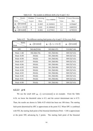
4.2.4.4 p=10
We use the small shift  0,0,0,0,0,0,0,0,0,11 μ as an example. From the Table
4-42, we know the threshold value is 0.5, and the correct determinant rate is 0.646667.
Then, the results are shown in Table 4-43 which has been run 100 times. The starting
fault point determined by SPC is approximate at the point 518. When SPC is combined
with NN, the starting fault point of the binomial distribution Prob. =1.00 is approximate
at the point 513, advancing by 5 points. The starting fault point of the binomial
distribution Prob. =0.99 is approximate at the point 507, advanced by 11 points. So
the starting fault point of the binomial distribution Prob. =0.90 is approximate the point
502, advanced by 16 points. Thus when the quality characteristics p=10, and the shift
is small, the model can find the starting fault point earlier.
This is the same method used for the larger shift ]0,5.1,0,1,0,5.0,0,1,0,5.0[1 μ and the

96. 85
all shifts  5.1,5.0,1,1,5.1,5.1,5.0,5.0,1,11 μ cases. Since we previously assumed the
starting fault point is number 501, we cannot find the starting point after combining NN.
The results are all the same from Prob.=0.99 to Prob.=0.90. As mentioned above, the
determined effect of SPC in combination with NN in the big shift and all shift cases do
not appear when the shift is small.
Therefore, when only using SPC chart in p=10 and =0.4, the starting fault point is
far from the assumed point 501. There is a small distance between the starting fault
point found by SPC in combination with NN and point 501, which we assumed for the
study. Different shifts will affect the time needed to determine the starting fault point.
To determine the time needed for a small shift  0,0,0,0,0,0,0,0,0,11 μ is more obvious
than to find it for the big shift ]0,5.1,0,1,0,5.0,0,1,0,5.0[1 μ and the all shifts
case  5.1,5.0,1,1,5.1,5.1,5.0,5.0,1,11 μ . In finding the standard deviation, we determine the
standard deviation in the big shift ]0,5.1,0,1,0,5.0,0,1,0,5.0[1 μ to be 1.81, and 15.89 for
the small shift  0,0,0,0,0,0,0,0,0,11 μ , which are shown in Table 4-43. We discover
that the standard deviation in the small shift is greater than for the big shift. That is to
say, the starting fault point of the shift ]0,5.1,0,1,0,5.0,0,1,0,5.0[1 μ is near the average
fault point, and the starting fault point of the shift  0,0,0,0,0,0,0,0,0,11 μ has a
greater distance from the average fault points.

97. 86
Table 4-42 The models in different shifts of p=10 and =0.4.
Models
Shifts
Hidden
Layer
Learning
Rate
Test RMSE
Threshold
Value
Correct
Determine
Rate
 0,0,0,0,0,0,0,0,0,11 μ 22 0.001 0.308062 0.4 0.646667
]0,5.1,0,1,0,5.0,0,1,0,5.0[1 μ 18 0.005 0.225005 0.5 0.866667
 5.1,5.0,1,1,5.1,5.1,5.0,5.0,1,11 μ 18 0.01 0.120946 0.5 0.966667
Table 4-43 The different starting fault points of p=10 and  =0.4 in every Prob.
Shifts
Prob.
 0,0,0,0,0,0,0,0,0,11 μ ]0,5.1,0,1,0,5.0,0,1,0,5.0[1 μ
SPC 517.88(15.89) 503.9(1.81)
Prob.=1.00 512.39(14.51) 502.18(1.79)
Prob.=0.99 506.41(10.05) 502.18(1.79)
Prob.=0.98 504.89(8.16) 502.18(1.79)
Prob.=0.97 503.49(5.57) 502.18(1.79)
Prob.=0.96 503.15(5.35) 502.18(1.79)
Prob.=0.95 502.26(2.86) 502.18(1.79)
Prob.=0.94 502.09(2.67) 502.18(1.79)
Prob.=0.93 502.05(2.68) 502.18(1.79)
Prob.=0.92 501.80(2.37) 502.18(1.79)
Prob.=0.91 501.70(2.25) 502.18(1.79)
Prob.=0.90 501.70(2.25) 502.18(1.79)

98. 87
Table 4-43 The different starting fault points of p=10 and  =0.4 in every
Prob.(Continued)
Shifts
Prob.
 5.1,5.0,1,1,5.1,5.1,5.0,5.0,1,11 μ
SPC 502.21(0.94)
Prob.=1.00 501.06(0.34)
Prob.=0.99 501.06(0.34)
Prob.=0.98 501.06(0.34)
Prob.=0.97 501.06(0.34)
Prob.=0.96 501.06(0.34)
Prob.=0.95 501.06(0.34)
Prob.=0.94 501.06(0.34)
Prob.=0.93 501.06(0.34)
Prob.=0.92 501.06(0.34)
Prob.=0.91 501.06(0.34)
Prob.=0.90 501.06(0.34)
4.3 Comparison of MEWMA Control Charts with Same
Quality Characteristics but Different  Values
As mentioned above, the result of advanced points in the middle shifts and big
shifts is not obvious. Therefore, we determine to compare with the small shifts that
have different quality characteristics to. We use the advanced value of SPC control
chart and Prob.=0.90 to make up the fields, because the points advanced most in the
accumulate probability of Binomial Distribution Prob.=0.90.

99. 88
4.3.1 p=2
Thus, we use  0,11 μ to explain. From Table 4-44, it can be observed that in
the different  value of small shift, they advanced 7, 4, 9 and 13 points individually.
And the discrepancy between the points determined by SPC that combine with NN is
imperceptible.
Table 4-44 The different  outcomes when p=2

Shifts
Prob.
 =0.1  =0.2  =0.3  =0.4
 0,11 μ  0,11 μ  0,11 μ  0,11 μ
SPC 509.75(7.84) 509.44(5.51) 510.71(9.32) 513.67(11.38)
Prob.=0.90 502.96(4.19) 505.07(3.42) 501.83(2.21) 506.26(8.23)
Advance Points 7 4 9 13
4.3.2 p=4
Accordingly, we use  0,0,0,5.01 μ to explain. We can see that in the different
 value of small shift, they advanced 10, 40, 7 and 22 points individually from Table
4-45. And the discrepancy between the points determined by SPC which combine
with NN is apparent.
Table 4-45 The different  outcomes when p=4

Shifts
Prob.
 =0.1  =0.2  =0.3  =0.4
 0,0,0,5.01 μ  0,0,0,5.01 μ  0,0,0,5.01 μ  0,0,0,5.01 μ
SPC 547.17(24.98) 540.46(29.86) 560.58(30.53) 571.8(69.15)
Prob.=0.90 537.83(22.96) 501(0) 553.34(29.97) 549.16(65.38)
Advance
Points
10 40 7 22

100. 89
4.3.3 p=6
Using  0,0,0,0,5.0,11 μ to explain, we can find out that in the different 
value of small shift, they advanced 3, 6, 2 and 5 points individually from Table 4-46.
And the discrepancy between the points determined by SPC which combine with NN is
not obvious.
Table 4-46 The different  outcomes when p=6

Shifts
Prob.
 =0.1  =0.2
 0,0,0,0,5.0,11 μ  0,0,0,0,5.0,11 μ
SPC 509.94(5.85) 511.38(7.23)
Prob.=0.90 506.6(5.90) 505.97(6.57)
Advance
Points
3 6
Table 4-46 The different  outcomes when p=6 (Continued)

Shifts
Prob.
 =0.3  =0.4
 0,0,0,0,5.0,11 μ  0,0,0,0,5.0,11 μ
SPC 511.46(5.80) 515.2(14.10)
Prob.=0.90 509.8(5.99) 510.47(11.63)
Advance
Points
2 5
4.3.4 p=10
We use  0,0,0,0,0,0,0,0,0,11 μ as an example. We can see Table 4-47 to
observe, that  = 0.1, 0.2, 0.3, and 0.4 of the small shifts they advanced 6, 7, 13 and 16
points individually. Because of it, we inference the bigger value is, the more evident
starting fault point determined by SPC which combine with NN is.

101. 90
Table 4-47 The different  outcomes when p=10

Shifts
Prob.
 =0.1  =0.2
 0,0,0,0,0,0,0,0,0,11 μ  0,0,0,0,0,0,0,0,0,11 μ
SPC 513.59(7.95) 513.33(9.23)
Prob.=0.90 507.79(8.02) 506.31(7.67)
Advance
Points
6 7
Table 4-47 The different  outcomes when p=10 (Continued)

Shifts
Prob.
 =0.3  =0.4
 0,0,0,0,0,0,0,0,0,11 μ  0,0,0,0,0,0,0,0,0,11 μ
SPC 516.73(13.16) 517.88(15.89)
Prob.=0.90 503.29(7.62) 501.70(2.25)
Advance
Points
13 16
4.4 Comparison and Contrast of the Result of Hotelling
T2
Control Chart and MEWMA Control Chart
According to the research above, we can find the starting fault point earlier and
more evident after combine the Hotelling
2
T control chart and MEWMA control chart
with NN. Nevertheless, it did not advanced obviously in the big shift. Therefore, we
will compare and contrast the results of the Hotelling
2
T control chart with MEWMA
control chart in different quality characteristics and small shift.
Situation 1: smaller p and small shift

102. 91
We use Hotelling
2
T control chart that p=3, and MEWMA control chart that p=2
and small shift to compare with each other while the shifts are  0,0,11 μ and
 0,11 μ . We can see Table 4-48; it advanced 13 and 16 points
individually when the  value in MEWMA control chart is 0.3 and 0.4. There is
no discrepancy with the Hotelling 2
T control chart. Nonetheless, when the  value in
MEWMA control chart is 0.1 and 0.2, it advanced 7 and 6 points. Although it has
some difference from the advanced points in Hotelling 2
T control chart, we understand
that Hotelling 2
T control chart would find the starting fault point earlier than the
MEWMA control chart.
As a result, we drew an inference that when the p gets bigger, MEWMA control
chart will find starting fault point earlier then Hotelling 2
T control chart. On the
contrary, when p numerary get smaller, Hotelling 2
T control chart will find the starting
fault points earlier than the MEWMA control chart.
Table 4-48 Comparison of Hotelling 2
T and MEWMA（Considering p and the shift
are small）
Control
Charts
Prob.
Hotelling 2
T
MEWMA（Different  ）
 =0.1  =0.2  =0.3  =0.4
SPC 515.58(17.53) 509.75(7.84) 509.44(5.51) 510.71(9.32) 513.67(11.38)
Prob.=0.90 501.55(3.54) 502.96(4.19) 505.07(3.42) 501.83(2.21) 506.26(8.23)
Advance
Points
14 6 7 13 16
Situation 2: larger p and small shift
We compare the larger quality characteristics in Hotelling
2
T control chart that
p=12 with MEWMA control chart that p=10 when the shifts are
 0,0,0,0,0,0,0,0,0,0,0,11 μ and  0,0,0,0,0,0,0,0,0,11 μ . In Table 4-49, due to the

103. 92
difference in SPC and the binomial distribution accumulate probability that Prob.=0.90
is the biggest, the starting fault points was found earlier obviously. Therefore, we
would use SPC and Prob.=0.90 to make the field. In the table, it’s clearly showed that
the starting fault point which advanced 13 and 16 points individually when the 
value in MEWMA control chart is 0.3 and 0.4 appeared earlier than the Hotelling
2
T control chart. However, when the  value in MEWMA control chart is 0.1 and
0.2, it advanced 7 and 6 points. It did not differ from the advanced points in Hotelling
2
T control chart greatly.
Table 4-49 Comparing of Hotelling 2
T and MEWMA（Considering p is larger
but the shift are small）
Control
Charts
Prob.
Hotelling 2
T
MEWMA（different  ）
 =0.1  =0.2  =0.3  =0.4
SPC 517.40(34.65) 513.59(7.95) 513.33(9.23) 516.73(13.16) 517.88(15.89)
Prob.=0.90 510.57(30.19) 507.79(8.02) 506.31(7.67) 503.29(7.62) 501.07(2.25)
Advance
Points
7 6 7 13 16

104. 93
Chapter 5 CONCLUSIONS AND FUTURE
RESEARCH
5.1 Conclusions
With the rise of living standards and progress in production techniques, people
have high expectations for product quality. In our research, we advocate using
multivariate control charts in combination with NN to monitor processes, and hope to
find the starting fault point in advance to use resources more efficiently. We used the
Hotelling 2
T and MWEMA control charts as examples, and took from them many
relevant assumptions. We have the continuity results: SPC in combination with NN
finds the starting fault points earlier than using the SPC chart alone for the different
shifts.
We use Hotelling 2
T control chart for an example. Table 5-1 shows that SPC in
combination with NN will better detect the starting fault point in the small shift case.
The Hotelling 2
T control chart cannot monitor the small shift well, so we use NN to
help us determine the starting fault point.

105. 94
Table 5-1 Different shift outcomes when using Hotelling 2
T control chart in
combination with NN
. Prob.
Shifts
SPC Prob.=1.0 Prob.=0.90
P=3
 0,0,11 μ 515.58(17.53) 503.36(7.63) 501.55(3.54)
 0,1,11 μ 504.34 501.78(3.69) 501.78(2.14)
 5.1,0,11 μ 501.69(1.03) 501(0) 501(0)
 1,5.0,5.01 μ 507.55(6.68) 503.20(4.92) 503.20(4.92)
 0,0,21 μ 501.15(0.66) 501.02(0.14) 501.02(0.14)
P=5
 5.0,5.0,5.0,5.0,5.01 μ 518.39(19.05) 512.73(17.8) 510.75(14.46)
 0,0,1,5.0,5.01 μ 510.65(9.82) 505.96(7.62) 505.96(7.62)
 0,0,0,0,11 μ 530.10(31.84) 518.98(25.54) 503.27(6.06)
 0,0,0,1,11 μ 505.60(6.15) 501.79(3.20) 501.79(3.20)
 0,0,0,0,21 μ 501.52(0.86) 501(0) 501(0)
P=8
 0,0,0,0,0,0,0,11 μ 539.97(48.49) 501.2(1.04) 501(0)
 5.1,5.0,1,0,0,0,0,01 μ 507.78(8.92) 501.85(3.57) 501.85(3.57)
 0,5.0,0,5.0,0,1,0,11 μ 505.30(5.05) 501.44(1.77) 501.44(1.77)
 0,0,5.0,5.0,1,1,5.1,5.11 μ 501.12(0.38) 501(0) 501(0)
 0,0,0,0,0,0,0,21 μ 501.05(0.22) 501(0) 501(0)
P=12
 0,0,0,0,0,0,0,0,0,0,0,11 μ 517.40(34.65) 514.72(34.20) 510.57(30.18)
 0,0,0,0,0,0,0,0,1,1,1,11 μ 501.46(0.89) 501.04(0.24) 501.04(0.24)
 0,0,0,0,0,0,5.1,5.1,1,1,5.0,5.01 μ 510.66(1.21) 501(0) 501(0)
 5.1,5.1,1,1,5.0,5.0,5.1,5.1,1,1,5.0,5.01 μ 501(0) 501(0) 501(0)
 0,0,0,0,0,0,0,0,0,0,0,21 μ 501.06(0.28) 501(0) 501(0)

106. 95
In MEWMA section, the starting fault point of  =0.1, 0.2 and 0.4 are
close, but  =0.3 is different, so we use  =0.2 and 0.3 to account for the
conclusion.
Because the MEWMA control chart is designed to monitor the smallest shifts of
the process, it can find the starting fault points effectively after combining with NN.
Especially in the shift  0,0,0,5.01 μ , there are a lot of advance points, which
are shown in Table 5-2. When =0.2 and p=4, the starting fault points of the small
shift  0,0,0,5.01 μ has great advanced by 40 points. Only when  =0.3, the
starting fault points has advanced by 10 points. However, the starting fault points
didn’t advance too much, it can precisely find out the starting fault points.
Table 5-2 Different shift outcomes when using MEWMA control chart in combination
with NN ( =0.2 and 0.3)
Advance Points
Shifts
MEWMA ( )
 =0.2  =0.3
P=2
 0,11 μ 4 9
 0,5.11 μ 2 1
 5.0,5.11 μ 2 3
P=4
 0,0,0,5.01 μ 40 7
 0,0,1,5.01 μ 2 9
 5.1,5.1,1,11 μ 1 2
P=6
 0,0,0,0,5.0,11 μ 6 2
 5.1,5.0,0,0,5.0,5.11 μ 2 2
 1,1,1,1,1,11 μ 2 2
P=10
 0,0,0,0,0,0,0,0,0,11 μ 7 13
]0,5.1,0,1,0,5.0,0,1,0,5.0[1 μ 2 1
 5.1,5.0,1,1,5.1,5.1,5.0,5.0,1,11 μ 1 1

107. 96
5.2 Future Research
(1) Utilizing the combination mechanism in practice.
We discussed how utilizing multivariate control charts in combination with NN can
detect the starting fault point earlier than only using SPC chart in the research.
Provided that one can suitably apply this in enterprise, it will meet their demands.
There are still a lot of development spaces for multivariate control charts that we can
explore in the future.
(2) Developing the information system
In the research, we used two types of software, including SAS and Q-net. Since
use of the software takes a lot of time and manpower, and since the manipulations are
inconvenient, we hope that we can develop a new program which is fast and efficient to
assist us doing the research. It not only saves time and costs, will also be useful for
future developments.
(3) Enhancing the identification rate of the neural networks
In this research, we observe methods of predicting starting error points in advance.
Nevertheless, the NN models still have room for improvement. If we can increase the
rate of correct error point determination, and decrease number of faults, we can vastly
improve quality and efficiency. This is not only good for business; it also provides an
opportunity for us to improve our research methods and monitoring techniques.

108. 97
(4) Constructing a general NN model
The NN models in our research are assumed to be the shifts of a known process.
However, in practice, there are fewer situations for which the shifts of the process are
known. In a real situation, we may not know which model to use. Therefore, we need
to develop NN models which can be used in every kind of process.

109. 98
REFERENCES
1. 尤志峰，「多變量管制圖非隨機性模型之辨識：應用類神經網路」，
東海大學工業工程研究所，1994 年。
2. 尤志峰，「類神經網路應用於多變量品質管制非機遇性模型之研
判」，東海大學工業工程研究所，1994 年。
3. 邵曰仁，侯家鼎，「使用 S 管制圖及 MLE 法以分辨階梯式改變干
擾產生啟始點之研究」，工業工程學刊 21:4，2004 年 7 月，頁
349-357。
4. 莊寶鵰，「MEWMA 管制圖的製程分析及診斷」，國立屏東技術學
院學報 6:2，1997 年 6 月，頁 147-151。
5. 莊寶鵰，「多變量 T2
管制圖的應用」，品質管制月刊 32:6，1997 年
6 月，頁 63-66。
6. 陳俊錫，「應用類神經網路偵測多變量製程變異性變化之研究」，元
智大學工業工程研究所，1996 年。
7. 黃聖蕙，「模糊理論與類神經網路應用於管制圖之研究」，元智大學
工業工程研究所，1997 年。
8. 葉怡成，「應用類神經網路」，台北；儒林圖書有限公司，1995。

110. 99
9. 歐筱華，「類神經網路應用於多變量統計製程管制之研究」，1994
年。
10. 駱景堯，池文海和唐文彥，「類神經網路在多變量品質管制
之研究」，品質學報，第 5 卷 第 1 期，1998 年，頁 1 – 25。
11. 顧瑞祥，「製程數據的非常態性對以類神經網路辨識管制圖異常之
影響」，工業工程學刊 19:6，2002 年 11 月，頁 13-22。
12. 顧瑞祥 謝益智，「類神經網路在管制圖異當的辨識與分析上的應
用」，技術學刊 12:3，1997 年 9 月，頁 523-529。
13. Alloway, J. A. Jr. and Raghavachari, M.” An Introduction to Multivariate Control
Charts”. Annual Quality Congress, Milwaukee WI, (45), 1991 , pp. 773-783.
14. ALT, F. B. “Multivariate Control Charts” in Encyclopedia of Statistical Sciences,
(6), 1985 (S. Kotz y N.L. Johson, Eds. Wiley, New York).
15. APARISI, F. “Hotelling 2
T control chart with adaptive sample sizes”,
International Journal of Production Research, (34), 1996, pp.2853-2862.
16. Alt, F. B. and Smith N. D. "Multivariate Process Control" in Handbook of Statistics
edited by P. R. Kirishnaiah and C.R. North-Holaand, Amsterdam, (7), 2000, pp.
333-351.
17. Fuchs, C. and Benjamini. Y. "Multivariate Profile Charts for Statistical Process
Control". Technometrics, (3), 1994, pp. 182--195
18. Hotelling, H, “Multivariate Quality Control” in Techniques of Statistical Analysis,
(Eds. C. Erisenhart, M. Hastay yW. A. wallis, McGraw-Hill), 1947, pp.111-184.
19. Hopfidld, J. J., “Neural Networks and Physical Systems with
Emergent Collective Computational Abilities,” Processings of the

111. 100
National Academy of Sciences, (79), 1982, pp. 2554 – 2558.
20. Hebb D. O. “The Organization of Behavior”, Wiley, 1949.
21. Jolayemi, J. K., “A Power Function Model Fordetermining Sample Size For the
Operations of Multivariate Control Chart,” Computational statistic &data analysis,
(20), 1995, pp. 633-641
22. Lowry, C. A., Woodall, W. H., Champ, C. W. and Rigdon, S. E. "A Multivariate
Exponentially Weighted Moving Average Control Chart". Technometrics, (34),
1992, pp. 46-53.
23. Lowry, C.A., and Montgomery, D. C., “A Review of Multivariate
Control Charts,” IIE Transactions, (27), 1995, pp. 800-810.
24. Montgomery, D. C., Keats, J. B., Runger, G. C. and Messina, W. S.
“Integration Statistical Process Control and Engineering Process
Control,” Journal of Quality Technology, (26), 1994.
25. Minskey M. and Seymour A. P. “Perceptrons”, MIT Press, 1969 (Enlarged edition,
1988).
26. Minsky. M.L. “Neural Nets and the Brain Model Pproblem”, Ph. D. dissertation,
Princeton University, Princeton, New Jersey, 1954.
27. Montgomery, D. C., Introduction to Statistical Quality Control, 5th edition, John
Wiley & Sons, New York, 2005 (1st edition, 1985, 2nd edition, 1991, 3rd edition,
1996, 4nd edition, 2001).
28. Mason, R. L. and Young C. J. “Improving Thesensitivity of the 2
T Statistic in
Multivariate Process control,” Journal of Quality Technology, (31), 1999, pp.
155-165.
29. Mason, R. L., Chou Y. M. and Young J. C. “Applying Hotelling’s 2
T Statistic to
Batch Processes”, Journal of Quality Technology, (33), 2001, pp. 466-479.

112. 101
30. Roberts, S.W. “Control Chart Tests Based on Geometric Moving Averages,”
Technometrics, (1), 1959, pp. 239-250.
31. Reynolds, M. R. Jr. and Stoumbos Z. G. “The SPRT Chart for Monitoring a
Proportion,” IIE Transactions, (30), 1998, pp.545-561.
32. Rosenblatt, F., “The Perceptron: A Probabilistic Model for Information Storage and
Organization in the Brain, Cornell Aeronautical Laboratory”, Psychological
Review, (65), 1958, pp. 386-408.
33. Runger. G. C. and Prabhu, S.S."Designing a Multivariate EWMA Control Chart".
Journal of Quality Technology, (29), 1997, pp. 8-15.
34. Sullivan, J. H. and Woodall, W. H. "A Comparison of Multivariate Control
Charts for Individual Observations". Journal of Quality Technology, (28), 1996, pp.
398-408.
35. Werbos, P. J. “Beyond Regression: New Tools for Prediction and Analysis in the
Behavioral Sciences”, Ph.D. Dissertation, Committee on Applied Mathematics,
Harvard University, Cambridge, MA, 1974.