2. R.Y. Chenavaz, G. Feichtinger and R.F. Hartl et al. / European Journal of Operational Research 284 (2020) 990–1001 991
general demand formulation, which accounts for nonlinearities and
dynamics in response to quality changes.
Our main results are as follows. First, we generalize the condi-
tion of Dorfman and Steiner (1954) in a dynamic context, stress-
ing the profit-maximizing conditions for the price–advertising,
price–quality, and advertising–quality relationships. Second, we de-
velop the pricing–advertising–quality relationship, examining the
conditions under which better quality triggers higher or lower
price and advertisement. Third, a phase diagram analysis learns
that quality develops monotonically in time and converges to a
unique steady state. We also show that quality investment could
either decrease or increase over time but this depends on its ef-
fectiveness. Such results foster the understanding of more com-
plex marketing-mix opportunities, enhancing the profitability of
the firm.
The paper is organized as follows. Section 2 presents the
related contributions. Section 3 develops the model, whereas
Section 4 generalized the rules of Dorfman–Steiner to a dynamic
context. Section 5 studies the impact of quality on dynamic pricing
and advertising. Section 6 computes the optimal trajectories using
a phase plane analysis, and Section 7 concludes.
2. Related contributions
Dynamic marketing-mix research provide numerous related
contributions. Such contributions focusing on dynamic pricing, ad-
vertising, and product quality, are regularly surveyed. Some of
these surveys focus on pricing (Dockner et al., 2000; Jørgensen
& Zaccour, 2012; Den Boer, 2015) and others on advertising
(Feichtinger et al., 1994; Bagwell, 2007; Huang et al., 2012;
Jørgensen & Zaccour, 2014). More specific literature pointers have
been provided recently for the price–quality relationship (Chenavaz
2017a; Vörös, 2019; Ni & Li, 2019) and for the advertising–quality
relationship (Chenavaz & Jasimuddin, 2017).
We now briefly review research using optimal control, which
provide elements about the relationships between price, quality,
and advertising. Table 1 presents in chronological order some of
the main optimal control models discussed below. The table helps
to understand the distinguishing mathematical formulation and
managerial interests in the literature, and thus the positioning of
our research.
Price and advertising are examined together by Piga
(2000) with a model of sticky prices with advertising, Helmes,
Schlosser, and Weber (2013) with oligopolistic strategies, and
Schlosser (2017) the stochastic element at the demand side. An
entertainment event is investigated by Jørgensen, Kort, and Zaccour
(2009), a marketing channel by Amrouche, Martín-Herrán, and
Zaccour (2008), and product diffusion by Helmes and Schlosser
(2015).
Price and quality are jointly studied as follows: Vörös (2006),
Chenavaz (2011, 2012), and Vörös (2013) consider improvement in
productivity. Teng and Thompson (1996) and Mukhopadhyay and
Kouvelis (1997) look at the joint dynamic pricing and quality poli-
cies, where quality is chosen by the firm. Reference effects are
considered by Gavious and Lowengart (2012), Xue, Zhang, Tang,
and Dai (2017), Chenavaz and Paraschiv (2018), and product re-
turns by De Giovanni and Zaccour (2020). The conditions deter-
mining when a product better quality is more or less expensive
are studied in Chenavaz (2017a), and generalized through the in-
troduction of goodwill by Ni and Li (2019) and through the salvage
value by Vörös (2019). The joint effects of price and quality invest-
ment are also considered when there is a potential competitor (Ha,
Long, & Nasiry, 2015), when there exists risk-averse attitude (Xie,
Yue, Wang, & Lai, 2011), and with the addition of a new channel in
a supply chain (Chen, Liang, Yao, & Sun, 2017). Eventually, Karaer
and Erhun (2015) and Cui (2019) analyze the role of product qual-
ity and pricing in preventing market entrant.
Advertising and quality are jointly analyzed in the following
contributions. Colombo and Lambertini (2003) look at product
differentiation. El Ouardighi, Feichtinger, Grass, Hartl, and Kort
(2016a,b) focus the role of word of mouth. More recently, Chenavaz
and Jasimuddin (2017) investigate when a product of better quality
increases or decreases advertising. In this last research, and close
to our contribution, price is assumed to be given by an inverse
demand function (see Table 1), that is price is not directly con-
trolled by the firm. In practice though, the firm, which differen-
tiates its product by leveraging the quality and advertising levels,
has also some freedom in price setting. There it has to take into ac-
count that setting the price in turn affects the advertising–quality
relationship (Chenavaz & Jasimuddin, 2017), which generalize to
a price–advertising–quality relationship (this article). Also, from a
conceptual point of view, Chenavaz and Jasimuddin (2017) proves
Tellis and Fornell’s (1988) conjecture about the advertising–quality
relationship, whereas this article generalizes Dorfman and Steiner’s
(1954) condition to a dynamic situation.
Only few contributions combine pricing, advertising, and qual-
ity, opposing tow by two. In this respect Fruchter (2009) looks
at decisions of price and advertising with perceived quality, in-
troducing a psychological element. Caulkins et al. (2015) analyze
history dependence with experience quality. Recently, Ni and Li
(2019) consider the carry-over effect role of goodwill in the price–
quality relationship, without investigating the price–advertising–
quality relationship. Also, as it appears in Table 1, most approaches
remain parametric, offering stronger, but less general results.
To the best of our knowledge, no research examine both the
price–advertising–quality relationship explicitly, that is with price,
advertising, and quality being all control or state variables and
with general (structural) formulations for both the demand func-
tion and state dynamics, imposing only little restriction on the re-
lationships among the variables. In this article, we bridge the gap
providing an optimal control model, which simultaneously address
these two points. Our results offer a deeper understanding of the
price–advertising–quality relationship in a general framework.
3. Model formulation
3.1. Model development
The intertemporal behavior of a monopolist is modeled in an
optimal control setting. The planning horizon is infinite and the
time t ∈ [0, ∞) is continuous.
3.1.1. Quality
At each time t, the firm chooses the level of quality investment
u(t) ∈ R+ that improves product quality q(t) ∈ R+. Thus, invest-
ment in quality u(t) is a decision (or control) variable and qual-
ity q(t) is a state variable. In other words, quality is modeled as a
system state.
The quality dynamics evolve according to
˙
q(t) = K(u(t), q(t)) with q(0) = q0, (1)
where K : R2
+ → R+ is twice continuously differentiable.1 The in-
tegration of (1) yields the cumulative level of quality q(t) = q0 +
t
0 K(u(s), q(s))ds. To simplify presentation, we shall omit the ar-
guments from the functions whenever there is no confusion, espe-
cially the temporal argument t.
1
The notations ˙
z and zx state for the time derivative of z and the first order
derivative of z with respect to x; the notations zxx and zxy denote the second order
derivative of z with respect to x and the cross derivative of z with respect to x
and y.
3. 992 R.Y. Chenavaz, G. Feichtinger and R.F. Hartl et al. / European Journal of Operational Research 284 (2020) 990–1001
Table 1
Selected optimal control models of price, advertising, and quality.
References System dynamics Main contributions
Teng and Thompson (1996) ˙
s = S(p, q, s) Show the different possible relationships between price p
and quality q
Piga (2000) ˙
p = s[α + β
aj −
Qj − p] Integration of advertising in a sticky price duopoly
Fruchter (2009) ˙
q = αp + βa − δq Focus on the impact of perceived quality and the pricing
and advertising policies
Caulkins et al. (2011) ˙
G = α(βp − G) Investigate the pricing policy for conspicuous goods when
goodwill exerts influence
Gavious and Lowengart (2012) ˙
rq = β(q − rq ) Role of reference quality in the pricing and quality policies
Chenavaz (2012) ˙
q = Q(uq, q) Show the impact of production cost and product quality on
˙
c = C(uc, c) the pricing policy
Caulkins et al. (2015) ˙
M = a/Mθ Role of market potential in the marketing-mix policy of
−δ(M − αp)(qmax − q) − βM price, advertising, and quality
Feng, Zhang, and Tang (2015) ˙
g = a − δg Role of goodwill and inventory dynamics in the
˙
i = −(α − βp + γ g) − δi marketing-mix policy of price and advertising
El Ouardighi et al. (2016a) ˙
p = c Role of costly price adjustment on sales and advertising
˙
s = α[β + a]s[(γ − θs) − p] − δs policies
El Ouardighi, Feichtinger, Grass, Hartl, and Kort (2016b) ˙
q = u(1 − q) Role of quality improvement and advertising policies
˙
s = {[(α + βa)q − β(1 − q)](1 − s/M) investment on product diffusion
−[1 − (1 − δq)]}s
Pan and Li (2016) ˙
q = uq − δqq Role of process-product innovation on the pricing policy
˙
c = uc − δcc
Chenavaz (2017a) ˙
q = Q(u, q) Show why a product of better quality may be less expensive
Chenavaz and Jasimuddin (2017) ˙
q = Q(u, q) Show when advertising increases or decreases with better
product quality
Chenavaz and Paraschiv (2018) ˙
r = β(p − r) Show when the selling price increases or decreases with the
˙
i = −D(p, r) reference price for a general demand function
Vörös (2019) ˙
q = αu Differentiate between strategic and non-strategic quality in
the price–quality relationship
Ni and Li (2019) ˙
q = Q(u, q) Role of advertising policy and goodwill in the price–quality
˙
g = G(a, q, g) relationship
Notes. We use the following unified notations for the variables: a, advertising; c, production cost; D, demand; g, goodwill; i, inventory; M, market potential; q, product
quality; Q, output; r, reference price; s, sales; u, investment. Also, j is a firm index and α, β, γ , δ are positive parameters.
Investment in quality u increases quality q with diminishing re-
turns and quality decreases autonomously, capturing the aging of
technology.
Ku 0, Kuu 0, Kq 0. (2)
These assumptions encompass the parametric instances ˙
q = u −
δq and ˙
q =
√
u − δq, with the constant rate of decay δ 0, as in
Jørgensen and Zaccour (2012) and Xue et al. (2017).
3.1.2. Cost
The unitary production cost function C : R+ → R+ is twice con-
tinuously differentiable and increases with quality q. Therefore the
cost is C = C(q) with
Cq 0. (3)
A similar cost formulation is used in Xue et al. (2017) and
De Giovanni and Zaccour (2020). The independence of cost to qual-
ity Cq = 0 and the increase of cost with quality Cq 0 describe, for
example, the software and hardware industries (Chenavaz, 2017a).
3.1.3. Demand
The firm decides at each time t the price level p(t) ∈ R+ and
the advertising expense a(t) ∈ R+. Quality is defined here as a
search (or design) attribute, which is easily knowable by search and
for which consumers prefer more than less. The demand function
D : R3
+ → R+ is twice continuously differentiable. The demand D
depends jointly on price p, advertising a, and quality q, that is
D = D(p, a, q).
Demand reduces with price. Demand rises with advertising
with diminishing returns. Demand increases with product quality.
It is more difficult to increase demand with more advertising and
better quality when price is high. There is a synergy phenomenon
between advertising and quality, that is, the impact of advertising
Table 2
Notations.
t = time,
r = interest rate,
p(t) = unit price at time t (control variable),
a(t) = advertising expense at time t (control variable),
u(t) = quality investment at time t (control variable),
q(t) = product quality at time t (state variable),
˙
q(t) = dq(t)/dt = K(u, q) = quality dynamics at time t,
λ(t) = current-value adjoint variable at time t,
C(q) = unit production cost,
D(p, a, q) = demand,
π(p, a, u, q) = [p − C(q)]D(p, a, q) − a − u = current profit,
H(p, a, u, q, λ) = current-value Hamiltonian
(quality) on demand is greater with greater quality (advertising).
Dp 0, Da 0, Daa 0, Dq 0, Dpa 0, Dpq 0, Daq 0. (4)
This general demand function places little restriction on the
way price, advertising, and quality affects demand. Indeed, this de-
mand function is compatible with the persuasive and informative
views (Bagwell, 2007; Chenavaz Jasimuddin, 2017). The persua-
sive view posits that advertising changes consumer preferences;
the informative view supposes that advertising provides product
information. In each case, greater advertising boosts demand.
3.2. Model analysis
Table 2 defines the notations used in the model analysis.
The current profit π with values in R writes
π(p, a, u, q) = [p − C(q)]D(p, a, q) − a − u. (5)
It appears now clearly that quality and advertising share similar
features, both stimulating demand and implying a cost. The essen-
tial differences are that (1) advertising directly implies a fixed cost
4. R.Y. Chenavaz, G. Feichtinger and R.F. Hartl et al. / European Journal of Operational Research 284 (2020) 990–1001 993
a whereas quality indirectly creates a fixed cost via quality invest-
ment u and (2) quality also generates a variable cost C(q).
The firm maximizes the intertemporal profit (or total present
value of profit) by simultaneously finding the optimal trajecto-
ries of pricing, advertising, and quality investment over the plan-
ning horizon. The firm accounts for the quality dynamics and the
discount rate r ∈ R+. Formally, the objective function of the firm
reads
max
p,a,u
∞
0
e−rt
π(p, a, u, q)dt, (6)
subject to ˙
q = K(u, q), with q(0) = q0. (7)
The intertemporal profit maximization problem is solved with
the necessary and sufficient optimality conditions of Pontryagin’s
maximum principle. On this basis, the shadow price (or current-
value adjoint variable) λ(t) represents the marginal value of quality
on the intertemporal profit at t, and the current-value Hamiltonian
H writes
H(p, a, u, q, λ) = [p − C(q)]D(p, a, q) − a − u + λK(u, q).
The current-value Hamiltonian H sums the current profit (p −
C)D − a − u and the future profit λK. As such, H measures the in-
tertemporal profit.
The maximum principle implies the dynamic of the shadow
price λ:
˙
λ = rλ − Hq = rλ − [−CqD + (p − C)Dq + λKq], (8)
with the transversality condition for a free terminal state and infi-
nite terminal time lim
t→∞
e−rt λ(t) = 0.
The intertemporal value at time t of a marginal increase in
quality q is given by the integration of (8) with the transversality
condition, computing
λ(t) =
∞
t
e−(r−
Kqdμ)(τ−t)
[(p − C)Dq − CqD]dτ, (9)
where we abuse the notation by denoting ∫Kqdμ for
∞
τ−t Kq(u(μ), q(μ))dμ.
Assuming the existence of an interior solution for advertising
and investment in quality, the monopolist maximizes the intertem-
poral profit H if and only if p, a, and u satisfy the necessary first-
order conditions:
Hp = 0 ⇒ D + (p − C)Dp = 0, (10a)
Ha = 0 ⇒ (p − C)Da − 1 = 0, (10b)
Hu = 0 ⇒ Ku −
1
λ
= 0. (10c)
Asterisk denoting optimality, let p∗(a, u) be the price that ver-
ifies (10a). This price maximizes the intertemporal profit of any
levels of advertising and quality investment. Similarly, a∗(p, u) and
u∗(p, a) denote the advertising rate satisfying (10b) and (10c); they
maximize the intertemporal profit for any level of price and qual-
ity investment and for any level of price and advertising. The maxi-
mum of the intertemporal profit is achieved when the firm chooses
together a price, advertising, and quality investment triple such
that (p∗, a∗, u∗) = (p∗(a∗, u∗), a∗(p∗, u∗), u∗(p∗, a∗)). We omit now
the asterisk notation, all equations referring to the optimal solu-
tion if not otherwise stated.
For the necessary first order conditions on H (10a)–(10c) to
yield a maximizing solution, assuming its existence, a sufficient
second order condition is the concavity of H. H is concave if and
only if the Hessian matrix is semi-negative definite, that is2
Hpp 0, (11a)
Hpp Hpa
Hap Haa
0, (11b)
Hpp Hpa Hpu
Hap Haa Hau
Hup Hua Huu
0, (11c)
with
Hpp = 2Dp − (p − C)Dpp, (12a)
Haa = (p − C)Daa, (12b)
Huu = λKuu, (12c)
Hpa = Hap = Da + (p − C)Dpa, (12d)
Hpu = Hup = 0, (12e)
Hau = Hua = 0. (12f)
Recall that H builds on functions all assumed to be twice con-
tinuously differentiable. Therefore, all partial derivatives of H are
themselves differentiable, and Schwarz’s theorem applies (Hij = Hji
for all i, j = p, a, u, q).
Eq. (12e) states that in the intertemporal profit H there are no
interaction effects between price and investment in quality. Sim-
ilarly, Eq. (12f) implies that with respect to H there are also no
interaction effects between advertising and quality investment.
Substituting (10a) into (12a) and recalling (11a) implies
2 − D
Dpp
D2
p
0, (13)
which dictates that D cannot be too convex in p in the sense that
the second order derivative of D with respect to p cannot be too
large. Such an assumption has been widely used in the literature
(see for example Kalish, 1983; Dockner et al., 2000; Vörös, 2006;
2019;Chenavaz, 2012; 2017b; Jørgensen and Zaccour, 2012; and Ni
Li, 2019).
Substituting (10b) into (12b) and recalling (11a) and (11b)
implies
−
Daa
D2
a
0, (14)
which is verified because of (4).
Conditions (11a)–(11c) together imply that λKuu ≤ 0, which, to-
gether with (2), leads to
λ(t) 0, ∀t ∈ [0, ∞), (15)
meaning that greater quality always increases the intertemporal
profit.
4. Generalizing the rules of Dorfman–Steiner
In this section, we generalize the static rules of Dorfman and
Steiner (1954) in a dynamic context, looking at the dynamic price–
advertising–quality relationship. The rules of Dorfman and Steiner
(1954) have to be verified for levels of price and advertising to be
candidate as optimal values. As such, these rules provide a useful
benchmark against which potential price and advertising levels can
be evaluated.
2
If all inequalities hold strictly, the Hessian matrix is strictly negative definite, H
is strictly concave, and the solution is unique.
5. 994 R.Y. Chenavaz, G. Feichtinger and R.F. Hartl et al. / European Journal of Operational Research 284 (2020) 990–1001
We first posit elasticity notations. Let ηp ≡ −Dp
p
D be the price
elasticity of demand, ηa ≡ Da
a
D the advertising elasticity of de-
mand, and ηq ≡ Dq
q
D the quality elasticity of demand.
Conditions (10a) and (10b) imply p − C = − D
Dp
and p − C = 1
Da
.
From these equalities and (9), we obtain that
DDa + Dp = 0, (16a)
λ(t) =
∞
t
e−(r−Kq )(τ−t)
D
ηq
ηp
p
q
−
dC
dq
dτ, (16b)
λ(t) =
∞
t
e−(r−Kq )(τ−t)
ηq
ηa
a
q
−
dC
dq
D
dτ. (16c)
Eq. (16a) assembles the first-order conditions on price and ad-
vertising. Eqs. (16b) and (16c) measure the future profit at t of an
additional unit of quality in terms of (1) price and quality effects
and (2) advertising and quality effects.
4.1. Dorfman–Steiner’s rules if future quality matters
Proposition 1. For a general demand function D = D(p, a, q), the
price–advertising, price–quality, and advertising–quality relationships
are characterized by
a
pD
=
ηa
ηp
, (17a)
ηq
ηp
p
q
dC
dq
, (17b)
ηq
ηa
a
q
dC
dq
D, (17c)
in which (17a) is a necessary and sufficient condition and (17b)–(17c)
are not necessary but sufficient conditions.
Proof. See Appendix B.1.
Equality (17a) represents what is well-known as the condition
of Dorfman and Steiner (1954). This condition stipulates that price
and advertising are such that the ratio of advertising to revenue
equals the ratio of elasticities of demand with respect to advertis-
ing and price. Inequalities (17b) and (17c) represent sufficient con-
ditions. Inequality (17b) states that price and quality are such that
the increase in the price that consumers are willing to pay after
a quality increase exceeds the unit increase in the cost of qual-
ity. Inequality (17c) exposes that advertising and quality are such
that the adjustment in advertising following a quality increase out-
weighs the total increase in the cost of quality. For exhaustiveness,
we derive the three conditions of Dorfman and Steiner (1954) and
compare them with our results in Appendix A.
The classical condition of Dorfman–Steiner (17a) is robust in our
dynamic setting where the firm considers future quality. We revisit
now this condition by explicitly showing the dependence of the
dynamics of price, quality, and advertising.
4.2. Dorfman–Steiner’s condition in dynamics
The condition of Dorfman–Steiner in (17a) provides the static
pricing–advertising condition. Proposition 1 shows that this con-
dition holds in a dynamic setting in which the future impact of
quality is considered by the firm. Note that this static condition
does not directly accounts for product quality. Though this condi-
tion must hold during the whole planning period, on which the
firm has an optimal behavior. At the optimum, if quality changes,
then marginal revenue variations balance marginal cost variations.
Such variations in quality also generate variations in pricing and
advertising. The link between the dynamics of pricing and adver-
tising on the one side and quality on the other side becomes ex-
plicit with the following proposition:
Proposition 2. For a general demand function D = D(p, a, q), the dy-
namics of the condition of Dorfman–Steiner (17a) is characterized by
˙
p
⎛
⎝−DpDa
14. −
⎞
⎠. (18)
Proof. See Appendix B.2.
Proposition 2 quantifies the link between the dynamics of
price and advertising and the dynamics of quality when the
condition of Dorfman–Steiner (17a) is verified. In other words,
Proposition 2 stresses the role of quality within the condition
of Dorfman–Steiner, which focuses on the pricing–advertising
relationship.
Eq. (18) is undetermined as the system state, quality, is known,
and the controls, price and advertising, are unknown. Still, this
proposition provides some insights on the consequences of qual-
ity variation on the level of price and advertisement. It shows that
quality impacts both pricing and advertising in an additive separa-
ble manner and it measures the linkage between the impacts on
price and advertising.
The signs of the three parentheses in Proposition 2 are un-
known. Therefore, when quality increases, price and advertising
may both increase or decrease together, or the one may increase
while the other decreases. If advertising is constant, price may in-
crease or decrease after a quality increase. Similarly, if price is con-
stant, advertising may raise or fall following better quality.
5. Quality impact on dynamic pricing and advertising
In this section we examine the impact of better quality on price
and advertising policies, when the rules of Dorfman and Steiner
(1954) studied in the previous section apply. The optimal pricing
and advertising policies have to hold at any time of the planning
period. Thus, we consider the time derivative of (10a) and (10b).
Rearranging terms offers
˙
p[2Dp + (p − C)Dpp] + ˙
a[Da + (p − C)Dpa]
= ˙
q[−Dq − (p − C)Dpq + CqDp], (19a)
˙
p[Da + (p − C)Dap] + ˙
a[(p − C)Daa]
= ˙
q[−(p − C)Daq + CqDa]. (19b)
Recall Hpp, Haa, and Hpa from (12a), (12b), and (12d) and
observe Hpq = −CqDp + (p − C)Dpq + Dq and Haq = −CqDa + (p −
C)Daq. By identification, the precedent equations synthesize to
˙
pHpp + ˙
aHpa = − ˙
qHpq, (20a)
˙
pHap + ˙
aHaa = − ˙
qHaq. (20b)
Eqs. (19a) and (19b) express the impact of quality on price and
advertising at the highest structural level. The dynamics of the
control variables p and a appear on the left hand-side and the dy-
namics of the state variable q show on the right hand-side. Fur-
ther, investment in quality u plays no direct role in the dynamics
15. R.Y. Chenavaz, G. Feichtinger and R.F. Hartl et al. / European Journal of Operational Research 284 (2020) 990–1001 995
Table 3
Synthesized marketing-mix implications of Proposition 3.
Case Condition Implication
1 −HkqHll + HlqHkl 0 sign ˙
k = sign ˙
q
2 −HkqHll + HlqHkl 0 sign ˙
k = − sign ˙
q
3 −HkqHll + HlqHkl = 0 sign ˙
k = unknown
Notes. Indexes k, l = p, a and k
16. = l.
of price and advertising; investment plays only an indirect role via
quality determination, as imposed by (10c).
Recall Hap = Hpa and define H2 = HppHaa − (Hpa)2. Note H2 ≥ 0
because of (11b). If H2 = 0, then the dynamics of p and a are un-
known. If H2 0, then the dynamics of p and a are characterized
as follows.
Proposition 3. For a general demand function D = D(p, a, q), the
impact of increased quality on the dynamics of price and advertising
is given by
˙
p =
−HpqHaa + HaqHpa
H2
˙
q, ˙
a =
−HaqHpp + HpqHap
H2
˙
q,
where H2 0.
Proof. See Appendix B.3.
The dynamic pricing and advertising policies given by
Proposition 3 are symmetrical since Hap = Hpa. Therefore, a syn-
thetic rule writes
˙
k =
−HkqHll + HlqHkl
H2
˙
q with k, l = p, a and k
17. = l,
for which the marketing-mix implications are synthesized in
Table 3.
Results in Proposition 3 synthesized in Table 3 have the fol-
lowing interpretations. On the one hand, the firm is better off
when price and advertising expense increase with quality, provided
−HkqHll + HlqHkl 0 with k, l = p, a and k
18. = l (Case 1). In Case 1,
price and advertising are complementary to quality. On the other
hand, if −HkqHll + HlqHkl 0 (Case 2), then the firm makes higher
profit by decreasing price and advertising effort after a quality in-
crease. In Case 2, price and advertising are substitute to quality. Fi-
nally, if −HkqHll + HlqHkl = 0 (Case 3), the firm adopts pricing and
advertising schemes for which the evolution is not tied to quality
dynamics. In Case 3, price and advertising are independent from
quality.
Further, Proposition 3 implicitly posits that the dynamics of
price and the dynamics of advertising may not be inferred from
each other. In other words, knowledge of price or advertising dy-
namics constitutes no signal for advertising or price dynamics
respectively.
6. Computation of the optimal trajectories
We start out with analyzing our deterministic model. After-
wards, we provide an extension where the horizon date, T, is finite
and stochastic.
6.1. Analysis of the deterministic model
We analyze the model (6) and (7) presented in Section 2 with
profit function (5), namely
max
p,a,u
∞
0
e−rt
[(p − C(q))D(p, a, q) − a − u]dt, (21)
subject to ˙
q = K(u, q), with q(0) = q0, (22)
employing a two-step approach since the “static” controls a and p,
do not enter the state dynamics.
In Step 1 we maximize the integrand
π(p, a, u, q) = (p − C(q))D(p, a, q) − a − u
with respect to the “static” controls a and p, yielding an optimal
profit function
π∗
(u, q) = max
a,p
π(p, a, u, q),
and optimal control functions p(q) and a(q). Then, in Step 2, we
solve an optimal control problem with state variable q and one
control variable u. This optimal control problem can be expressed
as
max
u
∞
0
e−rt
[(p(q) − C(q))D(p(q), a(q), q) − a(q) − u]dt,
subject to ˙
q = K(u, q), with q(0) = q0,
In order to solve this problem, we use the following specifica-
tions. First, we employ the linear demand function
D(p, a, q) = γ q + θ
√
a − βp. (23)
We also assume that C(q) is linear, i.e.,
C(q) = cq. (24)
Furthermore, we impose that
K(u, q) = q−α√
u − δq, α 0. (25)
The motivation for expression (25) is as follows: first, note that
α 0 reflects the fact that it is more difficult to increase quality
if quality is already high. Second, we introduce the term
√
u, be-
cause now the control variable u enters the problem in a nonlinear
and concave way.
The next proposition summarizes the results of Step 1.
Proposition 4. Under the condition
β ≥
θ2
4
, (26)
price and advertising depend on quality in the following way:
p(q) =
2β − θ2
c + 2γ
4β − θ2
q, (27)
a(q) =
θ(γ − βc)
4β − θ2
2
q2
. (28)
Price increases in quality, if
β
θ2
2
−
γ
c
, (29)
whereas advertising always increases with quality.
Demand is proportional to quality:
D =
2β
4β − θ2
(γ − βc)q,
which is positive, if
γ − βc 0. (30)
Proof. See Appendix C.1.
Having determined the functions forms of p(q) and a(q), we are
ready to analyze the optimal control problem of Step 2. After some
straightforward calculations, the Step 2 problem becomes
max
u
∞
0
e−rt
[(q) − u]dt, (31)
subject to ˙
q = q−α√
u − δq, (32)
19. 996 R.Y. Chenavaz, G. Feichtinger and R.F. Hartl et al. / European Journal of Operational Research 284 (2020) 990–1001
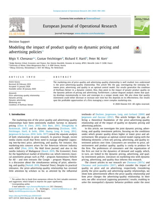
Fig. 1. Downward sloping saddle point path for α 1.
with
(q) =
(γ − βc)2
4β − θ2
q2
.
In Appendix C.2, we use the necessary optimality conditions for
this optimal control problem to obtain the canonical system in the
state-control plane:
˙
q = q−α√
u − δq,
˙
u = 2u(r + δ + αδ) − q1−α 2(γ − βc)2
4β − θ2
√
u.
It follows that there are two steady states, namely q = u = 0,
and a unique positive one:
ˆ
q =
(γ − βc)2
δ(r + δ + αδ)
4β − θ2
1
2α
, (33)
ˆ
u = δ2
(γ − βc)2
δ(r + δ + αδ)
4β − θ2
1+α
α
. (34)
In Appendix C.3, we investigate the stability properties of the
interior steady state (33) and (34), where we conclude that it is a
saddle point.
The two isoclines (relevant for the interior equilibrium) are
˙
q = 0 : u = (δq)2
, (35)
˙
u = 0 : u =
(γ − βc)2
(r + δ + αδ)
4β − θ2
2
q2(1−α). (36)
For 0 α 1 the ˙
u = 0 isocline is upward sloping in the (q, u)
plane, while it is downward sloping for α 1. In the hairline case
α = 1 it is horizontal.
In Fig. 1 we depict the case of a large α 1, where the sad-
dle point path is downward sloping just as the ˙
u = 0 isocline. For
low quality, high quality investments are undertaken in order to
improve it quickly.
In Fig. 2 we show the case of a small α 1, where the saddle
point path is upward sloping and so is the ˙
u = 0 isocline. For low
quality, also low quality investments are undertaken and quality
increases anyway.
Fig. 3 represents the hairline case of α = 1, where the saddle
point path is horizontal just like the ˙
u = 0 isocline. Quality in-
vestments are constant and do not depend on the current level of
quality.
To explain the qualitative differences between the three solu-
tions, consider Fig. 4. From this figure we conclude that for α 1,
Fig. 2. Upward sloping saddle point path for α 1.
Fig. 3. Horizontal for α = 1.
Fig. 4. The effectiveness of quality investment q−α, for α 1 (dashed), α = 1 (solid),
and α 1 (dotted).
quality investment is most effective when quality is small. This ex-
plains that quality investments decrease when quality goes up in
Fig. 1. For α 1, however, quality investment is relatively more ef-
fective when quality is large. This explains that quality investments
increase when quality goes up in Fig. 2.
6.2. Stochastic extension
Up to now, we had an infinite horizon. However, we are well
aware of the fact that the life cycle of a product is usually finite.
20. R.Y. Chenavaz, G. Feichtinger and R.F. Hartl et al. / European Journal of Operational Research 284 (2020) 990–1001 997
Moreover, it is hard to say beforehand when the economic life of a
product stops. For instance, it could be that there is some drastic
product innovation by some competitor making the current prod-
uct obsolete. To model this we impose that the life time of the
product, which we denote by T, is stochastic. Taking this into ac-
count, we reformulate the objective of the problem as follows:
max
p,a,u
ET
T
0
e−rt
[(p − C(q))D(p, a, q) − a − u]dt,
with ET denoting the expectation operator with respect to T. As-
suming an exponential distribution with parameter ρ 0 for T,
like in, e.g., Caulkins et al. (2011), the objective can ultimately be
rewritten into
max
p,a,u
∞
0
e−(r+ρ)t
[(p − C(q))D(p, a, q) − a − u]dt.
We conclude that now the complete problem looks as follows:
max
p,a,u
∞
0
e−(r+ρ)t
[(p − C(q))D(p, a, q) − a − u]dt. (37)
subject to ˙
q = K(u, q), with q(0) = q0. (38)
Comparing the problem (37) and (38) with the problem
(21) and (22) shows that they are equivalent except that in the
problem (37) and (38) the discount rate has increased by the rate
ρ, which makes the firm more myopic. From (35) and (36) we see
that the ˙
q = 0 isocline is not affected by a change in the discount
rate, while the ˙
u = 0 isocline moves downward if the discount rate
becomes larger. This results in less quality investments and a lower
long run quality level. We summarize these results as follows:
Proposition 5. (a) If the end of the life cycle of a product is finite and
exponentially distributed with parameter ρ, the problem is equivalent
to the original infinite horizon problem with the discount rate, r, being
increased by ρ.
(b) A larger value of r and/or ρ results in less quality investments
and a lower long run quality level.
6.3. Comparative statics
After having established how the long run equilibrium is af-
fected by the discount rate r, namely
∂ ˆ
q
∂r
0,
∂ ˆ
u
∂r
0,
we now investigate the effect of some other parameters. The re-
sults are summarized in the following proposition.
Proposition 6. (a) First we investigate the effect of γ , which mea-
sures the effect of quality on the market potential:
∂ ˆ
q
∂γ
0,
∂ ˆ
u
∂γ
0.
(b) Next we consider the effect of θ, which measures the effect of
advertising on the market potential:
∂ ˆ
q
∂θ
0,
∂ ˆ
u
∂θ
0.
(c) The next parameter we analyze is β, which is the slope of the
demand function:
sgn
∂ ˆ
q
∂β
= sgn
∂ ˆ
u
∂β
= sgn
θ2
2
−
γ
c
− β
.
(d) The next parameter to be investigated is c, being the unit cost
that positively depends on quality:
∂ ˆ
q
∂c
0,
∂ ˆ
u
∂c
0.
(e) If the depreciation rate of quality, δ, increases, the long run
optimal level of quality and quality investment react as follows:
∂ ˆ
q
∂δ
0,
∂ ˆ
u
∂δ
= −
(γ − βc)2
δ(r + δ + αδ)
4β − θ2
1
α
(γ − βc)2
×
r + 2δ + (2δ − r)α
α(r + δ + αδ)2
4β − θ2
.
Proof. See Appendix C.4.
The first result (a) is that the firm invests more in quality, if the
effect of quality on the market potential is bigger. Concerning re-
sult (b), the intuition is that advertising becomes more effective, so
that the firm advertises more when θ is larger. From our analysis
of Step 1, see (46), we have obtained that advertising and qual-
ity are complements. Hence the firm also invests more in quality.
According to result (c), the effect of the slope of the demand func-
tion, β, depends on the sign of θ2
2 −
γ
c − β. This is understand-
able, since from (29) we get that the same expression determines
whether price is increasing with quality or not. In particular we
obtain that if
θ2
2
−
γ
c
− β 0,
price is decreasing in quality. So, under this relationship we have
that an increase in β logically implies that the price is lower and
that the firm increases quality, which explains why an increase
in β results in a higher long run quality level and investment in
quality.
If c increases, according to result (d) the unit cost increases
more with quality and therefore the firm is reluctant to invest in
quality too much. According to result (e), we first see that if the
depreciation rate is bigger, the long run optimal quality level will
be lower. It is less clear what happens with the investment level.
Two effects can be distinguished. First, if quality depreciated more,
quality investments are less profitable, and therefore the firm in-
vests less. Second, if quality depreciates more, the firm has to carry
out more replacement investment to keep quality at a reasonable
level. Hence, ∂ ˆ
u
∂δ can have either sign. If α 1, or 2δ r, then the
first effect dominates, i.e., ∂ ˆ
u
∂δ 0.
7. Conclusion
In this research, we proposed a comprehensive, dynamic mod-
eling of price, advertising, and quality. The model is comprehen-
sive, yet with no sacrifice of generality, as it permits general (struc-
tural) functional forms for the cost and the relationships between
the marketing-mix variables at the demand level. On the basis of
an optimal control model, we offer analytic results. First, we gen-
eralize the classical condition of Dorfman and Steiner (1954) to a
dynamic context. Second, we provide the conditions along which
pricing and advertising strategies are aligned with or opposed
to quality improvement. These results help better understand the
profitable opportunities of the firm. Third, we obtain that quality
monotonically converges to a unique and positive steady state. On
this time path quality investment can either be increasing or de-
creasing, depending on how its effectiveness depends on the qual-
ity level itself.
Our research on the price–advertising–quality relationship may
be expanded into several ways. We could investigate a carry-over
role for advertising, which may have a lasting effect through good-
will formation. Further, to better characterize the dynamic behav-
ior of quality cost, quality could be modeled as a control variable,
and quality cost as a state variable. This modeling strategy would
deepen our understanding of cost dynamics, and its link to pric-
ing and advertising. Also, we may integrate temporal effects, such
21. 998 R.Y. Chenavaz, G. Feichtinger and R.F. Hartl et al. / European Journal of Operational Research 284 (2020) 990–1001
as fashion effects, in the demand function, which would also de-
pend directly on time. Eventually, profitable markets attract new
entrants, raising strategic issues. Consequently, it would be inter-
esting to model competition in our model. Such extensions will
allow to discuss the relationship between price, advertising, and
quality in a more complete way; they are left for future research.
This article provides significant insights into the choice of
the managerial variables over time. The general rule of pricing–
advertising–quality relationship, which we present, expands prior
results and formulates in a novel way the demand- and supply-
sides of the marketing-mix. Such a formulation, in turn, yields a
more comprehensive understanding of interplay between price, ad-
vertising, and quality. Our theoretical foundation calls for further
research to obtain empirical validation.
Appendix A. The rules of Dorfman and Steiner (1954)
We present here the rules of Dorfman and Steiner (1954) as
derived from profit maximization. For brevity, second-order con-
ditions are supposed to hold. Recall ηp the (absolute) price elastic-
ity of demand, ηa the advertising elasticity of demand, and ηq the
quality elasticity of demand.
A.1. The price–advertising relationship
The demand writes D = D(p, a) and the profit π = [p −
C(q)]D(p, a) − a. The first-order conditions πp = πa = 0 jointly im-
pose the rule of price–advertising
a
pD
=
ηa
ηp
. (39)
The price–advertising rule is the most well-known rule in
Dorfman and Steiner (1954, Section 1). For instance, this rule is
recalled in the survey of Bagwell (2007, Section 4.1.1).
A.2. The price–quality relationship
The demand is D = D(p, q) and the profit π = [p − C(q)]D(p, q).
The first-order conditions πp = πq = 0 in conjunction implicate the
rule of advertising–quality
dC
dq
=
ηq
ηp
p
q
. (40)
The price–quality rule originates in Dorfman and Steiner (1954,
Section 2). It appears later in Teng and Thompson (1996) and Lin
(2008).
A.3. The advertising–quality relationship
The demand is D = D(a, q) and the profit π = [p −
C(q)]D(a, q) − a, with p C a constant. The first-order condi-
tions πa = πq = 0 together dictate the rule of advertising–quality
dC
dq
D =
ηq
ηa
a
q
. (41)
The advertising–quality rule is not explicitly written in Dorfman
and Steiner (1954, Section 3). Also and to the best of our knowl-
edge, this rule has not been explicitly proposed in the litera-
ture. But the rule can be directly derived from the framework of
Dorfman and Steiner (1954) as above.
A.4. Comparison between Proposition 1 and the rules in Dorfman
and Steiner (1954)
For the sake of completeness, we compare Proposition 1 against
Dorfman and Steiner (1954). The famous condition of Dorfman and
Steiner (1954) in (39) characterizes the optimal policies of price
and advertising. More precisely, this condition describes the struc-
tural properties of these policies, linking the relative advertising
spending to the price and advertising elasticities of demand. This
condition has to hold for any couple of optimal price and adver-
tising policies, constituting a simple benchmark if the elasticities
hold constant. Also, numerous empirical studies have confirmed
the condition Dorfman and Steiner (1954) in different contexts.
Bagwell (2007) notes that this condition, though constraining, still
allows for freedom in the casual relationships between price and
advertising.
Dorfman and Steiner’s (1954)) rules (39)–(41) originate from
a static setting, whereas our rules (17a)–(17c) come from a dy-
namic setting. Simple comparison shows that their rules (with
strict equalities for any t over [0, ∞)) are a special case of our rules
(with weak inequalities over [t, ∞)). More precisely, the equality
of the price–advertising rule (39) is robust in our dynamic setting,
but the equalities of the price–quality and advertising–quality rules
(40) and (41) do not hold strictly in our setting.
Two reasons explain the difference between the two sets of
rules. First, in our setting, quality is a result of quality investment
and there is no restrictive optimality condition with respect to
quality. In contrast, in Dorfman and Steiner (1954), quality is di-
rectly chosen by the firm and there is an optimality condition with
respect to quality. Our modeling thus benefits from more freedom.
Second, our modeling refers to a dynamic framework where the
firm invests to increase future quality that will drive future profit;
quality has a future value for the firm. In contrast, their modeling
is static and the firm has only interest in current profit; quality
has no future value for the firm. Though, our modeling still en-
ables the equalities (40) and (41) to apply. In fact, these inequali-
ties hold (together) according to (16b) and (16c) if λ = 0, that is if
the future level of quality is of no interest for the firm maximiz-
ing the current intertemporal profit. In other words, if the firm be-
haves in a static way in the sense of considering only current profit
and disregarding future profit tied to future quality, then (17b) and
(17c) reduce to (40) and (41). In a nutshell, rules (17a)–(17c) differ
from (39) to (41) because (1) quality results from investment and
(2) future quality matters.
Appendix B. Mathematical details of Sections 4 and 5
B1. Proof of Proposition 1
Substituting the elasticity notation in (16a) and rearranging
yields the necessary and sufficient condition (17a). Recalling from
(15) that future quality increases future profit, that is λ(t) ≥ 0, to-
gether with the value of λ(t) measured in (16b) and (16c) impli-
cates the sufficient conditions (17b) and (17c).
B2. Proof of Proposition 2
Differentiate with respect to time the condition of Dorfman–
Steiner as expressed in (16a).
B3. Proof of Proposition 3
Solve Eqs. (20a) and (20b) with Cramer’s rule.
Appendix C. Mathematical details of Section 6
C.1. Proof of Proposition 4
Solving the Step 1 problem gives the first order conditions
πp = γ q + θ
√
a − 2βp + βcq = 0, (42)
22. R.Y. Chenavaz, G. Feichtinger and R.F. Hartl et al. / European Journal of Operational Research 284 (2020) 990–1001 999
πa = θ
p − cq
2
√
a
− 1 = 0. (43)
It is straightforward to check that the second order conditions
are satisfied (so that we indeed have developed conditions for a
maximum) if
πppπaa − π2
ap ≥ 0,
which holds if and only if (26) holds. Otherwise, concavity is vio-
lated and unbounded solutions might emerge.
We can solve (43) and (42) to obtain
p(q) =
2β − θ2
c + 2γ
4β − θ2
q, (44)
a(q) =
θ(γ − βc)
4β − θ2
2
q2
. (45)
From these expressions we get the dependence of price and ad-
vertising on quality,
p(q) =
2β − θ2
c + 2γ
4β − θ2
,
a(q) =
2θ2
4β − θ2
2
(γ − βc)2
q 0. (46)
We conclude that price increases in quality, if (29) holds,
whereas it always holds that the firm advertises more if the prod-
uct quality is higher.
Substitution of (44) and (45) into (23) learns that demand is
proportional to quality, i.e.
D =
2β
4β − θ2
(γ − βc)q,
and we conclude that positive demand only arises if
γ − βc 0, (47)
which completes the proof.
C.2. Derivation of the canonical system of the Step 2 problem
To solve the Step 2 optimal control problem (31) and (32), we
set up the Hamiltonian
H =
(γ − βc)2
4β − θ2
q2
− u + λ
q−α√
u − δq
.
Maximizing H with respect to u gives
λ = 2qα√
u, (48)
whereas the co-state equation satisfies
˙
λ = rλ − 2
(γ − βc)2
4β − θ2
q − λKq. (49)
We now establish the optimal trajectories in a state-control
phase diagram (q, u). To do so, we first differentiate (48) with re-
spect to time, which leads to
˙
λ = 2αq−1
u − 2δαqα√
u + qα 1
√
u
˙
u.
This can be combined with (49) and (48) to obtain the ˙
u equa-
tion:
˙
u = 2u(r + δ + αδ) − 2
(γ − βc)2
4β − θ2
q1−α√
u. (50)
C.3. Stability analysis of the interior steady state
We investigate the stability properties of the interior steady
state. The Jacobian of the canonical system
˙
q = q−α√
u − δq,
˙
u = 2u(r + δ + αδ) − q1−α 2(γ − βc)2
4β − θ2
√
u,
is
J =
⎡
⎢
⎢
⎣
−αq−1−α√
u − δ
1
2
√
u
q−α
−(1−α)q−α 2(γ −βc)2
4β−θ2
√
u 2(r + δ + αδ) − q1−α (γ − βc)2
4β − θ2
√
u
⎤
⎥
⎥
⎦,
(51)
with the determinant
det J = − 2α(r + δ + αδ)q−1−α√
u − 2δ(r + δ + αδ)
+ q1−α δ(γ − βc)2
4β − θ2
√
u
+
(γ − βc)2
4β − θ2
q−2α.
For the positive steady state (33) and (34), we have
det J = −2δα(r + δ + αδ) 0.
Hence, the interior steady state is a saddle point.
C.4. Proof of Proposition 6
(a) First we investigate the effect of γ :
∂ ˆ
q
∂γ
=
γ − βc
α
δ(r + δ + αδ)
4β − θ2
×
(γ − βc)2
δ(r + δ + αδ)
4β − θ2
1
2α −1
0,
∂ ˆ
u
∂γ
=
2(1 + α)(γ − βc)δ2
α
δ(r + δ + αδ)
4β − θ2
×
(γ − βc)2
δ(r + δ + αδ)
4β − θ2
1
α
0,
where the sign follows from (47).
(b) Next we consider the effect of θ:
∂ ˆ
q
∂θ
=
(γ − βc)2
θ
αδ(r + δ + αδ)
4β − θ2
2
×
(γ − βc)2
δ(r + δ + αδ)
4β − θ2
1
2α −1
0,
∂ ˆ
u
∂θ
=
2(1 + α)δ2
(γ − βc)2
θ
αδ(r + δ + αδ)
4β − θ2
2
×
(γ − βc)2
δ(r + δ + αδ)
4β − θ2
1
α
0.
(c) The next parameter we analyze is β:
∂ ˆ
q
∂β
=
2c
α
(γ − βc)
δ(r + δ + αδ)
θ2
2
− γ
c
− β
4β − θ2
2
×
(γ − βc)2
δ(r + δ + αδ)
4β − θ2
1
2α −1
,
23. 1000 R.Y. Chenavaz, G. Feichtinger and R.F. Hartl et al. / European Journal of Operational Research 284 (2020) 990–1001
∂ ˆ
u
∂β
= 4cδ2 1 + α
α
(γ − βc)
δ(r + δ + αδ)
θ2
2
− γ
c
− β
4β − θ2
2
×
(γ − βc)2
δ(r + δ + αδ)
4β − θ2
1
α
,
from which we obtain that it depends on the sign of θ2
2 −
γ
c − β
whether an increase of β will lead to higher quality investments
or not.
(d) The next parameter to be investigated is c:
∂ ˆ
q
∂c
= −
β(γ − βc)
αδ(r + δ + αδ)
4β − θ2
×
(γ − βc)2
δ(r + δ + αδ)
4β − θ2
1
2α −1
0,
∂ ˆ
u
∂c
= −
2(1 + α)β(γ − βc)δ
α(r + δ + αδ)
4β − θ2
×
(γ − βc)2
δ(r + δ + αδ)
4β − θ2
1
α
0.
(e) Finally, we consider δ:
∂ ˆ
q
∂δ
= −
(γ − βc)2
(r + 2δ + 2αδ)
2α(δ(r + δ + αδ))2
4β − θ2
×
(γ − βc)2
δ(r + δ + αδ)
4β − θ2
1
2α −1
0,
∂ ˆ
u
∂δ
= −
(γ − βc)2
δ(r + δ + αδ)
4β − θ2
1
α
(γ − βc)2
×
r + 2δ + (2δ − r)α
α(r + δ + αδ)2
4β − θ2
.
This completes the proof.
References
Amrouche, N., Martín-Herrán, G., Zaccour, G. (2008). Pricing and advertising of
private and national brands in a dynamic marketing channel. Journal of Opti-
mization Theory and Applications, 137(3), 465–483.
Bagwell, K. (2007). The economic analysis of advertising. Handbook of Industrial Or-
ganization, 3, 1701–1844.
Board, E. (2019). The murky world of Madagascar’s roaring vanilla trade. The
Economist. Retried on September 26, 2019, https://www.economist.com/news/
2019/07/05/the-murky-world-of-madagascars-roaring-vanilla-trade.
Caulkins, J., Feichtinger, G., Grass, D., Hartl, R., Kort, P., Seidl, A. (2011). Optimal
pricing of a conspicuous product during a recession that freezes capital markets.
Journal of Economic Dynamics and Control, 35(1), 163–174.
Caulkins, J. P., Feichtinger, G., Grass, D., Hartl, R. F., Kort, P., Seidl, A. (2015). His-
tory-dependence generated by the interaction of pricing, advertising and experi-
ence quality. Vienna University of Technology. Technical report research report
2015-05.
Chen, J., Liang, L., Yao, D.-Q., Sun, S. (2017). Price and quality decisions in
dual-channel supply chains. European Journal of Operational Research, 259(3),
935–948.
Chen, M., Chen, Z.-L. (2015). Recent developments in dynamic pricing research:
Multiple products, competition, and limited demand information. Production
and Operations Management, 24(5), 704–731.
Chenavaz, R. (2011). Dynamic pricing rule and RD. Economics Bulletin, 31(3),
2229–2236.
Chenavaz, R. (2012). Dynamic pricing, product and process innovation. European
Journal of Operational Research, 222(3), 553–557.
Chenavaz, R. (2017a). Better product quality may lead to lower product price. The
BE Journal of Theoretical Economics, 17(1), 1–22.
Chenavaz, R. (2017b). Dynamic quality policies with reference quality effects. Applied
Economics, 49(32), 3156–3162.
Chenavaz, R., Jasimuddin, S. (2017). An analytical model of the relationship be-
tween product quality and advertising. European Journal of Operational Research,
263, 295–307.
Chenavaz, R., Paraschiv, C. (2018). Dynamic pricing for inventories with ref-
erence price effects. Economics: The Open-Access, Open-Assessment E-Journal,
12(2018-64), 1–16.
Colombo, L., Lambertini, L. (2003). Dynamic advertising under vertical product
differentiation. Journal of Optimization Theory and Applications, 119(2), 261–280.
Cui, Q. (2019). Quality investment, and the contract manufacturerâs encroachment.
European Journal of Operational Research, 279(2), 407–418.
De Giovanni, P., Zaccour, G. (2020). Optimal quality improvements and pricing
strategies with active and passive product returns. Omega. forthcoming
Den Boer, A. V. (2015). Dynamic pricing and learning: Historical origins, current re-
search, and new directions. Surveys in Operations Research and Management Sci-
ence, 20(1), 1–18.
Dockner, E., Jorgenssen, S., Long, V. N., Gerhard, S. (2000). Differential games in
economics and management science. Cambridge University Press.
Dorfman, R., Steiner, P. O. (1954). Optimal advertising and optimal quality. The
American Economic Review, 44(5), 826–836.
El Ouardighi, F., Feichtinger, G., Grass, D., Hartl, R., Kort, P. M. (2016a). Au-
tonomous and advertising-dependent ‘word of mouth’ under costly dynamic
pricing. European Journal of Operational Research, 251(3), 860–872.
El Ouardighi, F., Feichtinger, G., Grass, D., Hartl, R. F., Kort, P. M. (2016b). Advertis-
ing and quality-dependent word-of-mouth in a contagion sales model. Journal
of Optimization Theory and Applications, 170(1), 323–342.
Elmaghraby, W., Keskinocak, P. (2003). Dynamic pricing in the presence of inven-
tory considerations: Research overview, current practices, and future directions.
Management Science, 49(10), 1287–1309.
Erickson, G. M. (1995). Differential game models of advertising competition. Euro-
pean Journal of Operational Research, 83(3), 431–438.
Feichtinger, G., Hartl, R. F., Sethi, S. P. (1994). Dynamic optimal control models in
advertising: Recent developments. Management Science, 40(2), 195–226.
Feng, L., Zhang, J., Tang, W. (2015). A joint dynamic pricing and advertising
model of perishable products. Journal of the Operational Research Society, 66(8),
1341–1351.
Flint, J. (2019). ATT operating chief defends media strategy build around stream-
ing, DirectTV. The Wall Street Journal. Retried on September 26, 2019,
https://www.wsj.com/articles/at-t-operating-chief-defends-media-strategy-
built-around-streaming-directv-11569355738
Fruchter, G. (2009). Signaling quality: Dynamic price-advertising model. Journal of
Optimization Theory and Applications, 143(3), 479–496.
Gavious, A., Lowengart, O. (2012). Price–quality relationship in the presence of
asymmetric dynamic reference quality effects. Marketing Letters, 23(1), 137–161.
Ha, A., Long, X., Nasiry, J. (2015). Quality in supply chain en-
croachment. Manufacturing Service Operations Management, 18(2),
280–298.
Helmes, K., Schlosser, R. (2015). Oligopoly pricing and advertising in isoelastic
adoption models. Dynamic Games and Applications, 5(3), 334–360.
Helmes, K., Schlosser, R., Weber, M. (2013). Optimal advertising and pricing in a
class of general new-product adoption models. European Journal of Operational
Research, 229(2), 433–443.
Huang, J., Leng, M., Liang, L. (2012). Recent developments in dynamic advertising
research. European Journal of Operational Research, 220(3), 591–609.
Jørgensen, S., Kort, P. M., Zaccour, G. (2009). Optimal pricing and advertising poli-
cies for an entertainment event. Journal of Economic Dynamics and Control, 33(3),
583–596.
Jørgensen, S., Zaccour, G. (2012). Differential games in marketing: 15. Springer Sci-
ence Business Media.
Jørgensen, S., Zaccour, G. (2014). A survey of game-theoretic models of coopera-
tive advertising. European Journal of Operational Research, 237(1), 1–14.
Kalish, S. (1983). Monopolist pricing with dynamic demand and production cost.
Marketing Science, 2(2), 135–159.
Karaer, Ö., Erhun, F. (2015). Quality and entry deterrence. European Journal of Op-
erational Research, 240(1), 292–303.
Lin, P.-C. (2008). Optimal pricing, production rate, and quality under learning ef-
fects. Journal of Business Research, 61(11), 1152–1159.
Mukhopadhyay, S. K., Kouvelis, P. (1997). A differential game theoretic model for
duopolistic competition on design quality. Operations Research, 45(6), 886–893.
Ni, J., Li, S. (2019). When better quality or higher goodwill can result in lower
product price: A dynamic analysis. Journal of the Operational Research Society,
70(5), 726–736.
Nuttall, C. (2019). The UK milestones for a driverless future. Financial
Times. Retried on September 26, 2019, https://www.ft.com/content/
9883e3fa-ce69-11e9-99a4-b5ded7a7fe3f.
Pan, X., Li, S. (2016). Dynamic optimal control of process–product innovation with
learning by doing. European Journal of Operational Research, 248(1), 136–145.
Piga, C. A. (2000). Competition in a duopoly with sticky price and advertising. In-
ternational Journal of Industrial Organization, 18(4), 595–614.
Schlosser, R. (2017). Stochastic dynamic pricing and advertising in isoelastic
oligopoly models. European Journal of Operational Research, 259(3), 1144–
1155.
Sethi, S. P. (1977). Dynamic optimal control models in advertising: A survey. SIAM
Review, 19(4), 685–725.
Tellis, G. J., Fornell, C. (1988). The relationship between advertising and product
quality over the product life cycle: A contingency theory. Journal of Marketing
Research, 25(1), 64–71.
Teng, J.-T., Thompson, G. L. (1996). Optimal strategies for general price-quality de-
cision models of new products with learning production costs. European Journal
of Operational Research, 93(3), 476–489.
24. R.Y. Chenavaz, G. Feichtinger and R.F. Hartl et al. / European Journal of Operational Research 284 (2020) 990–1001 1001
Vörös, J. (2006). The dynamics of price, quality and productivity improvement deci-
sions. European Journal of Operational Research, 170(3), 809–823.
Vörös, J. (2013). Multi-period models for analyzing the dynamics of process im-
provement activities. European Journal of Operational Research, 230(3), 615–623.
Vörös, J. (2019). An analysis of the dynamic price-quality relationship. European
Journal of Operational Research, 277(3), 1037–1045.
Xie, G., Yue, W., Wang, S., Lai, K. K. (2011). Quality investment and price decision
in a risk-averse supply chain. European Journal of Operational Research, 214(2),
403–410.
Xue, M., Zhang, J., Tang, W., Dai, R. (2017). Quality improvement and pricing
with reference quality effect. Journal of Systems Science and Systems Engineering,
26(5), 665–682.