Analysis Of Poverty In Indonesia With Small Area Estimation : Case In Demak District

1. Proceeding - Kuala Lumpur International Business, Economics and Law Conference Vol. 3.
November 29 - 30, 2014. Hotel Putra, Kuala Lumpur, Malaysia. ISBN 978-967-11350-4-4
52
ANALYSIS OF POVERTY IN INDONESIA WITH SMALL AREA ESTIMATION : CASE IN DEMAK DISTRICT
Setia Iriyanto
Faculty of Economics, University of Muhammadiyah Semarang Indonesia
E-mail : setiairiyanto_se@yahoo.com
Moh. Yamin Darsyah
Faculty of Mathematics and Sciences, University of Muhammadiyah Semarang Indonesia
E-mail : mydarsyah@yahoo.com
ABSTRACT
This study is aimed to analyze poverty with method “Small Area Estimation” in Demak district. This study also used the method of linear regression analysis with the dependent variable number of poor families and the independent variable percentage of the number of farm households (X1), the percentage of household water taps users (X2) and population density (X3). Data were collected from the Central Bureau of Statistics in 2013. “Small Area Estimation” Method is applied to estimate the poverty mapping to the district level in Demak. The results of poverty mapping in Demak shows that the population density becomes the dominant factor of poverty in some areas of Demak.
Keywords : small area estimation, poverty mapping, population density
I. Introduction
Poverty is the characteristic of regional variations. Factors such as natural disaster trends, distribution and quality of land, access to education and health facilities, level of infrastructure development, employment opportunities, and so forth are some causes of poverty.Measurement of poverty through sample surveys can not directly produce the aggregation size at a low level (eg. district/sub-district, village) due to the limitations of the data so then as one of the solution is to use small area estimation.Small area estimation is a statistical technique to estimate the parameters sub-population of small sample size.The estimation techniques use the data from a large domain such as census data and susenas data to estimate the variables of concern to the smaller domain.Simple estimation on a small area that is based on the application of the sampling design model (design-based) referred to as the direct estimation where the direct estimation is not able to provide sufficient accuracy when the sample size in the area was small so that the resulting statistics will have a large variant or even the estimation can not be done because the resulting estimates are biased (Rao, 2003).
As an alternative estimation techniques to increase the effectiveness of the sample size and decrease the error then developed the indirect estimation techniques to perform estimation on a small area with adequate precision. This estimation technique is performed through a model that connects related areas through the use of additional information or concomitant variables. Statistically, the method by utilizing the additional information would have the nature of "borrowing the strength" from the relationship between the average small area and the additional information.All indirect estimation techniques have assumed a linear relationship between the average small area with concomitant variables that are used as additional information in the estimation.Various small area estimation techniques that are often used such as Empirical Bayes, Hirarical Bayes, EBLUP, synthetic, and composite approach which all using parametric procedures.If there is no linear relationship between the average small area and the concomitant variables then it is not right to "borrow the strength" from other areas by using a linear model in the indirect estimation.To overcome this problem, then developed a non-parametric approach.One of the non-parametric approach that is used is Kernel Approach.
Various studies relating to Small Area Estimation with a non-parametric approach such as Darsyah and Wasono (2013a) The Estimation of IPM On A Small Area In The City Of Semarang With A Non-parametric Approach, Darsyah and Wasono (2013b) The Estimation Of The Level Of Poverty In Sumenep District With SAE Approach,Darsyah (2013) Small Area Estimation Of The Per-capita Expenditure In Sumenep District With Kernel- Bootstrap Approach, Opsmer (2005) Small Area Estimation Using Penalized Spline, Mukhopadhay and Maiti (2004) Small Area Estimation With A Non-parametric Approach.

2. Proceeding - Kuala Lumpur International Business, Economics and Law Conference Vol. 3.
November 29 - 30, 2014. Hotel Putra, Kuala Lumpur, Malaysia. ISBN 978-967-11350-4-4
53
II. Theory
To be able to measure poverty, BPS uses the concept of the ability to meet basic needs (basic needs approach).Through this concept of poverty is seen as an economic inability to meet the basic needs of both food and non-food which measured in terms of per-capita expenditure,with this approach, it can be calculated by the percentage of the poor population towards the total of population. Distinguishing between the poor and non-poor is the poverty line.
There are two main problems in small area estimation.The first problem is how to generate an accurate estimation with a small sample size in a domain or a small area.The second problem is how to estimate the Mean Square Error (MSE). The solution of the problem is to "borrow the information" from both inside the area, outside the area, and outside the survey.In most applications of small area estimation, it used the assumptions of linear mixed models and the estimation was sensitive to this assumption.If the assumption of linearity between the average small area and concomitant variables are not met, then "borrow the strength" from other areas by using the linear model is not appropriate.Mukhopadhyay and Maiti (2004) using a model as follow:
(1)
(2)
m(xi) is smoothing function that defines the relation between x and y.θi is the average of unobservable small area, yi is the direct estimation of the average small area sampled,yi is the direct estimation of the average small area sampled,ui is error random variables which independent and identically distributed with E(ui) = 0 and var(ui) = ,and εi independent and identically distributed with E(εi) = 0 and var(εi) = Di,In assuming Di is known. The substitution of equation (1) and (2) will result in the following equation:
(3)
To estimate m(xi), Mukhopadhyay and Maiti (2004) using Kernel Nadaraya-Watson Estimation
(4)
Where is a kernel function with bandwidth h and .
Kernel function that is often used is the normal function (Hardle, 1994). Estimators over the linear towards yi, can be written as:
(5)
Where
Based on the above definition, the best estimate of the average small area θi is
(6)
Where and
an estimator of .
(7)
MSE estimation for small area:
(8)
However, the above estimation MSE has a weakness because the information is lost and there is no fixed formula, then to estimate the MSE can be done with the following equation of bootstrap approach:
(9)
where J is the number of bootstrap population, is mean estimators of small area to- i from bootstrap population to- j and is the true value of the average small area to- ifrom bootstrap population to- j.

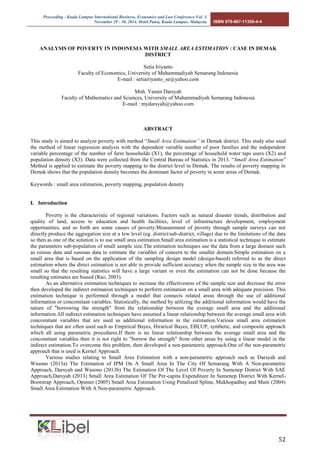
3. Proceeding - Kuala Lumpur International Business, Economics and Law Conference Vol. 3.
November 29 - 30, 2014. Hotel Putra, Kuala Lumpur, Malaysia. ISBN 978-967-11350-4-4
54
III. Research Methods
1. The Source of Data
The Source of main data thatused in the study is secondary data drawn from the data of the National Socio-
Economic Survey (SUSENAS) BPS in 2013 and Demak District in Figures in 2013.The response variables in this
study is concern in poverty level which measured from per-capita expenditure at the level of sub-districts in Demak
District. Concomitant variables that thought to affect and describe poverty rate is the percentage of farm families
because most of the poor population (60 percent in 2013) was working in the agricultural sector (X1), the percentage
of water tap (PDAM) users (X2), and population density (X3).
2. Method Analysis
The stages in this study are:
1. Selecting concomitant X variables that affect/describing poverty level
2. Examination of normality assumption
3. Diversity test
4. Descriptive analysis
5. Testing the model
6. Mapping the poverty region
7. Analysis of povertymappingbased small area
IV. Results
The analysis that is used in this study is the Small Area Estimation (SAE) which will be processed using the
software R &Minitab.Response variables that used in this study is the percentage number of poor families in each sub-districts
in Demak District, while the predictor variables that used in this study is the percentage number of RTP (X1),
the percentage number of water taps users (X2), and population density (X3) in each sub-districts in Demak District.
a. The Examination of normality assumption
Examination of residual normality assumption using the Kolmogorov-Smirnov (KS) which produces KS value
of 0,113 with the p-values (>0,15) is greater than significant level 5%, so that obtained the decision of accept H0which
means that the.residualspread normally.
RESI1
Percent
-2 -1 0 1 2
99
95
90
80
70
60
50
40
30
20
10
5
1
Mean
>0,150
-3,86992E-15
StDev 0,7167
N 14
KS 0,113
P-Value
Probability Plot of RESI1
Normal
Figure 5.1
In Figure 5.1, it can be seen that the regression residual plots spread following a straight line which shows a residual
that spreads normally.
b. Spatial Diversity Test (Heteroskidastity)
Testing spatial diversity using Breusch-Pagan test (BP) produces a BP value of 6,76 with p-value (0,079) is
less than significant level 10%, so that obtained the decision of reject H0 which means that there are spatial variations
in the poverty data in every sub-district in Demak District 2012.The existence of spatial diversity on poverty shows
that every sub-district in Demak District has its own characteristics, so it takes a local approach to model and to
address the diversity that occurs on poverty.

4. Proceeding - Kuala Lumpur International Business, Economics and Law Conference Vol. 3.
November 29 - 30, 2014. Hotel Putra, Kuala Lumpur, Malaysia. ISBN 978-967-11350-4-4
55
c. Descriptive Analysis of Poverty Rate in Demak District and Factors Affecting
This descriptive analysis aims to provide an overview description of the average, variance, minimum, and maximum values on the response and predictor variables.
Table 5.2 below shows that the percentage number of poor families in Demak District has an average of 7,143 with a variance of 5,685, the minimum value of 3,287 and a maximum value of 11,026.As for the percentage number of RTP in Demak District has an average of 7,141 with a variance of 2,678, the minimum value of 5,03 and a maximum value of 9,872. For the percentage number of households that use water taps in Demak District has an average of 7,142 with a variance of 199,998, the minimum value of 0 and a maximum value of 2239. The population density in Demak District has an average of 1200,71 with a variance of 14105, the minimum value of 720 and a maximum value of 2239.
Table 5.2 Descriptive Statistics Poverty Rates and Factors Affecting
Variabel
Mean
Vari
ans
Minimum
Maximum
The Percentage Number of Poor Families (Y)
7,143
5,685
3,287
11,026
The Percentage Number of RTP (X1)
7,141
2,678
5,033
9,872
The Percentage Number of Households water taps user (X2)
7,142
199,998
0
51,531
Population density (X3)
1200,71
1410E5
720
2239
Table 5.3 shows that the estimated parameters of each X1 variable has a negative parameter coefficient of - 0,894 to 0,993 between the percentage of farm household variables (X1) with the percentage number of poor families (Y) that occurs in Bonang, Karanganyar, Mijen, and Wedung Sub-District.Negative values in the X1 variable indicate that there is a negative relationship between the variable of number percentage of RTP with the number percentage of poor families, which means that a reduced number of RTP in a region will reduce the number of poor families in the region. This occurs presumably because the number of RTP in the four sub-districts are fewer than the other sub- districts.
In Table 5.3, also noted that the value of the X2 variable has a negative parameter coefficient from -0,033 to 0,409 between the percentage number of household water taps users (X2) with the percentage number of poor families (Y) that occurs in all sub-districts in Demak District.Negative values of X2 variable indicate that there is a negative relationship between the variables percentage number of household water taps user with the percentage number of poor families, which means that the reduced number of household that use water taps in a region will reduce the number of poor families in the region.Supposedly, the number of household that use water taps have a inversely proportional relationship towards the number of poor families, which means that an increase in the number of water taps user will reduce the number of poor families, because the quality of water consumed will greatly affect to the life quality of the family.
R2 values that obtained from the model was 60,79%. This means that the diversity of the percentage number of poor families due to the percentage of poor households, the percentage number of household that use water taps, and a population density of 60,79%, while 30,21% were caused by other factors that influence poverty.

5. Proceeding - Kuala Lumpur International Business, Economics and Law Conference Vol. 3.
November 29 - 30, 2014. Hotel Putra, Kuala Lumpur, Malaysia. ISBN 978-967-11350-4-4
56
Table 5.3 Minimum and Maximum Value Parameter Estimation Model
Variable
Parameter Coefficient
Minimum
Median
Maximum
Intercept
1,727
2,468
11,240
X1
-0,894
0,021
0,993
X2
-0,033
-0,027
0,409
X3
0,0006
0,003
0,004
SSE
43,976
R2
60,79%
d. Testing Model
Goodness of fit or suitability testing for the model was conducted to determine the location of the factors that affect the level of poverty in Demak District.
Based on table 5.4, obtained the p value (0,042) which means that the p value is less than 5% of significant level (0,042 <0,05). This means reject H0 because the p value is less than 5% of significant level, which means that there is an influence of geographical factors in the model.
Table 5.4 Compliance Test Model
SSE
Df
Fcount
Pvalue
Model
43,977
9,023
2,775
0,042
Based on table 5.5, the results showed that there are 10 sub-districts were affected by population density variable (X3), and there are 4 districts which do not affect the three variables that used in this study. This is presumably because there are other variables that more significant besides the variable of percentage number of RTP, the percentage number of household that use water taps, and the population density towards the poverty level in 4 sub- districts in Demak District.
Table 5.5 Parameters Significant At The Model per Sub-District in Demak District
No
Sub-District
Variable
1
Mranggen
X1,2,3
2
Karangawen
X1,3
3
Guntur
X1,3
4
Sayung
X1,2,3
5
Karangtengah
X1,3
6
Demak
X1,2,3
7
Bonang
X1,3
8
Wonosalam
X1,3
9
Dempet
X3
10
Gajah
-
11
Karanganyar
-
12
Mijen
-
13
Wedung
-
14
Kebonagung
X1,3

6. Proceeding - Kuala Lumpur International Business, Economics and Law Conference Vol. 3.
November 29 - 30, 2014. Hotel Putra, Kuala Lumpur, Malaysia. ISBN 978-967-11350-4-4
57
V. Conclusion
The following conclusions were derived from the results of studies that have been done include:
a) Application of Small Area Estimation can be combine with Spatial Regression.
b) The variables that most affect towards the level of poverty in Demak District overall is population density although the percentage of the farm family was large enough
c) The location factor/inter-subdistrict area affect the rate of poverty in Demak District
d) R2 value obtained from the model of 60,79%. This means that the diversity of the percentage number of poor families due to the percentage of poor households, the percentage number of household users of water taps and a population density of 60,79%, while 30,21% were caused by other factors that influence poverty.
Suggestions for this research requires a lot of aspects of the approach to statistical methods in order to get more comprehensive results, namely:
a). The research that has been done can be developed by SAE Parametric Approach, GWR, Time Series Analysis, etc..
b) Instruments/research variables to be explored again in order to describe a more aggregate conditions
c) The results of this study are expected to be input to the Demak District Government (Bappeda) in making planning and regional development policies.
VI. Acknowledgements
We would like to thank to DIKTI. This research was funded by grants PDP DIKTI.
VII. Bibliography
[BPS]. Central Bureau of Statistics. 2013. http://www.bps.go.id/glossary/2013.
Darsyah, M.Y. (2013). Small Area Estimation terhadap Pengeluaran Per Kapita di Kabupaten Sumenep dengan pendekatan Kernel-Bootstrap. Statistict Journal UNIMUS. Vol.1 No.2 . Statistict Journal UNIMUS. Vol.1 No.2
Darsyah, M.Y dan Wasono, R (2013). Pendugaan Tingkat Kemiskinan di Kabupaten Sumenep dengan pendekatan SAE. Proceedings of the National Seminar on Statistics UII, Yogyakarta.
Darsyah, M.Y and Wasono, R (2013). Pendugaan IPM pada Area Kecil di Kota Semarang dengan Pendekatan Nonparametrik. Proceedings of the National Seminar on Statistics Diponegoro University, Semarang.
Hardle, W. (1994). Applied Non parametric Regression. New York: Cambrige University Press.
Mukhopadhyay P, Maiti T. 2004. Two Stage Non-Parametric Approach for Small Area Estimation. Proceedings of ASA Section on Survey Research Methods: 4058-4065.
Opsomer et al. 2004. Nonparametric Small Area Estimation Using Penalized Spline Regression. Proceedings of ASA Section on Survey Research Methods:1-8.
Rao JNK. 2003. Small Area Estimation. New Jersey : John Wiley &Sons, Inc.