ChinnIrwin International Economics, Chapter 13 (draft 76201.docx

Chinn/Irwin International Economics, Chapter 13 (draft
7/6/2017) © Menzie Chinn
1
13
Income and Interest Rates under Floating Exchange Rates, and
the International
Trilemma
Overview
In this chapter, we learn:
●●● How exchange rates adjust under floating exchange rates to
restore external equilibrium
●●● How fiscal and monetary policy affect output, exchange
and interest rates under floating
rates.
●●● How fiscal and monetary policy effectiveness differ under
floating and fixed rates.
●●● How a liquidity trap will prevent expansionary monetary
policy from increasing output.

●●● How effective fiscal and monetary policies are when
capital mobility is perfect under
different exchange rate regimes
●●● The International Trilemma means that an economy can
only simultaneously achieve two of
three goals of exchange rate stability, monetary independence
and financial integration
2
''It's a bleak picture,'' said Charles W. Bartsch, a policy analyst
with the
Northeast-Midwest Institute, a Washington-based center for
economic and
environmental research. ''Many of these towns aren't going to
make it. They're
going to have to go through bankruptcy and let the chips fall
where they
may.''
The municipalities' financial problems grow out of the severe
depression that
in recent years has savaged the country's steel industry, idling
more than
700,000 workers in this once prosperous region.

…
Hammered by the strength of the dollar, which made imported
steel less
expensive, and bypassed by the economic recovery, steel
companies have
closed one mill after another. Once the backbone of the region's
economy, the
mills are now silent, soot-stained monuments to another era.
From, Lindsay Gruson, New York Times, October 6, 1985.
This news article from the 1980’s is perplexing. The economic
recovery was well underway by
1985, and yet the industrial heartland was suffering with high
unemployment and shuttered
factories. How can a strong dollar be blamed for this outcome?
In fact, the dollar was a key reason for the rapid decline in the
industrial Midwest, and surging
imports was part of the story. How and why motivates the
development of this model with a
freely floating exchange rate.
In contrast to the model presented in Chapter 12, the central
bank in this model is no longer
committed to exchanging home currency for foreign currency at
a designated exchange rate.
Rather, the central bank eschews foreign exchange intervention,
and thus gains monetary policy
autonomy.
In terms of the model, foreign exchange reserves no longer

change in response to changes in
interest rates and trade flows. Instead, the exchange rate freely
adjusts in response to market
forces so as to keep foreign exchange reserves constant.
Because of this switch in what variable
is free to move and what is not, the model’s predictions differ
substantially from those obtained
in Chapter 12.
13.1 The Model
We retain the IS, LM and BP=0 schedules as described in the
previous chapter. One seemingly
minor -- but critical – distinction is that the q variable no
longer has a bar over it, indicating it is
no longer a fixed constant.
3
(13.2) <LM curve>
(13.3) ∗ <BP=0 curve>

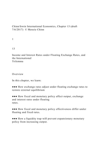
In the fixed exchange rate case, q is treated as a constant,
changed only when the central bank
decides to devalue or revalue the currency. In a floating
exchange rate case, q is an endogenous
variable, free to move in response to other forces. When the
equilibrium interest rate is above
(below) that consistent with external equilibrium, the currency
appreciates (depreciates) so as to
maintain the BP=0 condition. When the economy is at external
equilibrium (as below in Figure
13.1), then there is no tendency for q to change.
Figure 13.1: IS-LM-BP=0 in equilibrium
This graph is indistinguishable from Figure 12.1. The
differences from the fixed exchange rate
situation become apparent when one examines the implications
of fiscal and monetary policy.
13.2 Fiscal Policy under Floating Exchange Rates
We’ll examine fiscal and monetary policies in turn. First,
consider what happens if one increases
government spending.
LM
IS

i0
i
Y0 Y
4
Figure 13.2: Expansionary fiscal policy under floating exchange
rates, high capital mobility
The IS curve shifts out (dark gray arrow). Output initially rises
to Y1 and interest rates to i1.
However, now the equilibrium interest rate is greater than that
consistent with external
equilibrium; this means financial inflows exceed that necessary
to offset the trade balance. In the
fixed exchange rate system, this would mean increases in
official reserves. However, under the
floating exchange rate system, the home currency appreciates,
i.e., q falls.
As q falls, this affects two curves: the IS and the BP=0
schedules. Inspecting equation (13.1), one
sees that a fall in q shifts in the IS curve. Now examine
equation (13.3); a fall in q shifts up the
BP=0 curve. These two shifts are depicted in Figure 13.2 (light
gray arrows). Notice then that

equilibrium income falls to Y2 and interest rates to i2 (although
both of these are higher relative to
the initial starting values of Y0 and i0).
Why do these shifts occur? As q falls (appreciates), exports fall
and imports increase and hence
aggregate demand declines and the IS shifts in. As exports
decrease and imports increase for any
given income level with an appreciated currency, financial
inflows must be higher for any given
income level in order for external balance to hold. This can only
be accomplished by a higher
interest rate. This is the same as saying the BP=0 curve is
shifted higher.
In the end, in an open economy, some of the fiscal expansion is
offset by reduced “net exports”
(exports minus imports). Another way of thinking about this
phenomenon is that there is now an
additional channel for crowding out. There are now two interest
rate sensitive components of
aggregate demand: investment spending and net exports. Net
exports are not literally interest
sensitive, but to the extent that they depend upon the exchange
rate and the exchange rate is in
turn dependent upon interest rates, they are in effect interest
sensitive.
13.3 Monetary Policy under Floating Exchange Rates
Now we consider what happens if a monetary expansion is
undertaken. In this case, we examine
LM
'IS (increased gov’t spending)

i0
i
Y0 Y Y1
i1
"IS (increased gov’t
spending, appreciated
currency
Y2
i2
IS
5
only the high capital mobility case, as the qualitative results do
not depend on the degree of
financial openness.
In Figure 13.3 below, the monetary expansion shifts out the LM

curve (dark gray arrow). The
resulting equilibrium interest rate ii is less than required for
external equilibrium. As a
consequence, there is an incipient balance of payments deficit
and the exchange rate depreciates.
The depreciated exchange rate results in increased net exports,
so the required interest rate for
external equilibrium falls (the BP=0 curve shifts downward).
The increase in net exports also
means that domestic aggregate demand rises, and the IS curve
shifts out. The equilibrium settles
at income level Y2 and interest rate i2.
Figure 13.3: Expansionary monetary policy under floating
exchange rates, high capital mobility
Notice that monetary policy is relatively powerful. The increase
in the money supply decreases
the interest rate and hence spurs investment, thereby increasing
output. The lower interest rates
also puts negative pressure on the balance of payments, and
under a free float, this manifests
itself in a depreciation of the home currency. This shifts out the
BP=0 curve (light gray arrow)
This depreciation spurs exports and discourages imports, so the
expansionary monetary policy
“crowds in” net exports, as well as investment.
This result highlights the fact that in an open economy under a
floating exchange rate regime,
monetary policy is generally more powerful than in the case of a
closed economy. That is
because monetary policy can now exert its influence through
two channels – the investment

channel and the net exports channel. That is even more true the
greater the degree of financial
capital mobility.
The impact of monetary policy in this example highlights the
following fact that: although in a
fully floating exchange rate regime, market conditions
determine the currency’s value, that does
not mean the central bank (and the government) cannot
influence that value. In particular, the
'LM (monetary expansion)
IS
i0
i
Y0 Y Y2
i1
'IS (depreciated currency)
Y1
i2
LM

6
central bank can, by affecting the interest rate, affect the market
conditions that underlie the
exchange rate’s level.
13.4 Application: The Dollar and Deficits during the 1980’s
At the beginning of the Chapter, the problems of the industrial
heartland of America during the
mid-1980’s were recounted – declining manufacturing and high
unemployment. This experience
can be readily explained using the model we’ve just described.
When President Reagan came to office in January 1981, he
proposed increases in defense
spending and tax cuts which, along with the recession, caused a
large budget deficit. The budget
balance, when there is an income tax, is given by equation
(13.4):
(13.4)
≡ ̅
The official measure of the budget balance is a not a “pure”
measure of the stance of fiscal

policy, since tax receipts fall and spending on transfers such as
unemployment insurance rise
during recessions. A more exogenous measure of fiscal policy is
provided by the budget balance
evaluated at full employment, sometimes called the cyclically
adjusted budget balance. This
measure, along with the cyclically adjusted, normalized by GDP
and full employment GDP
(YFE), is shown in Chart 13.1.
Chart 13.1: Actual budget balance to GDP ratio (blue),
cyclically adjusted budget balance ratio (red) and
cyclically adjusted budget balance to potential GDP (green).
Source: Congressional Budget Office,
Budget and Economic Outlook, August 2011.
-.10
-.08
-.06
-.04
-.02
.00
.02
.04
70 75 80 85 90 95 00 05 10

Actual
Cyclically adjusted
Cyclically adjusted to
Potential GDP
Federal budget
balance to GDP
7
The increase in the cyclically adjusted budget deficit –
increased spending and decreased taxes –
by about 3 percentage points of GDP stimulated the economy.
In Figure 13.4, this effect is
represented by an outward shift in the IS curve (dark gray
arrow). At the same time, the Federal
Reserve under the leadership of Chairman Paul Volcker,
embarked upon a policy of squeezing
inflation out of the economy through contractionary monetary
policy. In terms of our model, this
results in the LM curve shifting inward (black arrow), so that
the interest rate rises to i1.
Assuming high capital mobility this leads to an appreciation of
the currency, which, as shown in
Figure 13.4 leads to shifts of the BP=0 and IS curves (light gray
arrows).

Figure 13.4: Expansionary fiscal policy and contractionary
monetary policy under flexible exchange rates,
high capital mobility
The economy settles at income level Y2, interest rate i2. The
income level exceeds the starting
level at Y0, but not by as much as would have been the case if
monetary policy had been less
contractionary. In this sense, the collision of expansionary
fiscal policy and contractionary
monetary policy is like stepping on the gas and brake pedals at
the same time.
The model also implies the resulting interest rate increase
should appreciate dollar. And that is
exactly what happened.
LM
'IS (increased gov’t spending)
i0
i
Y0 Y
i2

"IS (increased gov’t spending,
appreciated currency)
Y2
'LM (contractionary monetary policy)
IS
Y1
i1
8
Chart 13.2: Real interest rate (left scale) and log real value of
US dollar (1973M01=0). Real interest rate
calculated as difference between one year Treasury yield and
one year ex post inflation. Source: Federal
Reserve Board, and BLS.
From President Reagan’s inauguration to the dollar’s peak in
March 1985, the real value of the
currency rose by 35%. Then, as shown in Chart 13.3, starting in
1982, the US began running a
massive trade deficit, unprecedented in the post-War era,
largely because of the appreciated
dollar. Instead of fiscal policy crowding out investment, as

would have occurred in the closed
economy model, net exports were crowded out.
-8
-4
0
4
8
12
16
-.3
-.2
-.1
.0
.1
.2
.3
1975 1980 1985 1990 1995 2000 2005 2010
Real interest rate
[left scale]

Log real value
of US dollar
[right scale]
Reagan
9
-.4
-.3
-.2
-.1
.0
.1
.2
.3
.4
-.06

-.05
-.04
-.03
-.02
-.01
.00
.01
.02
1975 1980 1985 1990 1995 2000 2005 2010
Net exports
to GDP ratio
[right scale]
Log real value
of US dollar
[left scale]
Chart 13.3: Log real value of US dollar (1973M1=0), and net
exports as a share of GDP. Source: Federal
Reserve Board, and BEA.

The closely timed onset of deterioration in the budget and trade
balances led to the term “Twin
Deficits”, discussed in Chapter 9. In words, the appreciation of
the dollar made US exports
relatively uncompetitive in markets overseas, while it made
foreign made goods relative cheap to
American consumers and firms. As a consequence,
manufacturers were hit hard by the
combination of recession and then increased import
competition. The industrial cities of the
Midwest suffered so strongly that this experience led to the
coining of yet another term: “the
Rustbelt”.
Starting toward the end of 1984, Fed policy loosened
considerably. Combined with tax increases,
the US interest differential relative to other countries declined,
and so too did the dollar. With a
lag of a couple years (as shown in Chart 13.3), US net exports
responded to the dollar decline, so
that by 1986, the trade deficit shrank as a share of GDP.
13.5 Interest Rate Shocks
So far we have examined the effects of domestic policies.
However, the model is also quite
useful for examining how events in the rest of the world can
affect exchange rates and income at
home. For instance, mid-2014, expectations of a US interest rate
relative to that in the euro area
led to a depreciation of the euro against the US dollar.
We can analyze this event in the model from the perspective of
the euro area. Consider the

increase in the US interest rate as a rise in *i . Notice that in
Equation 13.3, *i enters in one-
10
for-one in the determination of the interest rate that equilibrates
the balance of payments.
If the foreign (US) interest rate rises (exogenously) by one
percentage point, then the BP=0 curve
will shift up one percentage point. The outcome in the high
capital mobility case is depicted
below in Figure 13.5.
Figure 13.5: RoW interest rate rises under floating exchange
rates
As the foreign interest rate rises (dark arrow), the euro area
interest rate rises above what is
consistent with external balance. The euro thus depreciates to q’
shifting down the BP=0 curve,
and shifting out the IS curve (light arrows). In the end, the euro
area interest rate rises in
response to the foreign interest rate increase, although not one-
for-one.
To stabilize the exchange rate, the monetary authority (in this
case the European Central Bank)

could raise euro area interest rates. In Figure 13.5, this would
entail a shift backwards of the LM
curve. In other words, the country could maintain the exchange
rate at a given level, at the cost
of losing control over output. In this case, the country would
undergo a recession. Since the euro
area was experiencing slow growth, the ECB did not tighten
monetary policy.
This episode illustrates the trade-offs that policymakers make.
While it might be provi desirable
stabilize the currency’s value, that has to be weighed against the
benefits of maintaining the level
of output.
13.6 Summarizing Effects under Fixed and Floating Exchange
Rates
Our examination of the effects of different policies, as well as
developments abroad, has yielded
a large number of outcomes, depending on exchange rate
regime, degree of capital mobility, and
whether the central bank sterilizes financial capital flows. The
following table summarizes these
many results, assuming relatively high capital mobility.
LM
IS
i0
i

Y0 Y
'IS (depreciated currency)
Y1
i1
igher foreign
interest rate)
depreciated currency)
11
Exchange rate
regime Income
Interest
rate
Real
exchange
rate

Trade
balance
Foreign
Exchange
Reserves
Government
spending
Fixed
(w/sterilization) Increase Increase No change Decrease
Increase
Fixed Increase Increase No change Decrease Increase
Floating Increase Increase Appreciation Decrease No change
Real money
supply
Fixed
(w/sterilization) Increase Decrease No change Decrease
Decrease
Fixed No change No change No change No change Decrease
Floating Increase Decrease Depreciation Increase No change
Real
exchange
rate
Fixed
(w/sterilization) Increase Increase Devaluation Increase
Increase

Fixed Increase Increase Devaluation Increase Increase
Floating nr nr nr nr nr
Foreign
interest rate
Fixed
(w/sterilization) No change No change No change No change
Decrease
Fixed Decrease Increase No change Increase Decrease
Floating Increase Increase Depreciation Depreciation
No change
Table 13.1: The Impact of Policies and Foreign Developments.
Notes: Responses of each variable in the
column to a change in the indicated variable in left column,
under fixed exchange rate regime with
sterilization, without sterilization, and free floating. Entries in
bold face italics indicate relatively large
changes. “nr” denotes “not relevant”.

12
Box 13.1: Empirical Estimates of Policy Effects
Theory provides insights into the effectiveness of fiscal,
monetary and
exchange rate policies in open economies. Under fixed
exchange rates,
fiscal policy should be relatively effective, monetary policy
relatively
ineffective (particularly in the longer term). The reverse is true
under
floating exchange rates: fiscal policy should be less effective,
and
monetary policy more effective, holding all else constant.
How well do these predictions hold in real world data? One way
to answer
this question is to compile data on a number of economies, and
examine
how changes in government spending affect output, the real
exchange
rate, and the current account.
Ethan Ilzetzki, Enrique Mendoza and Carlos Vegh estimated the
response
of these variables to an unexpected amount of government
spending

equal to one percent of GDP. In contrast to the Mundell-
Fleming model
we’ve examined, these estimates allow the central bank to react
to the
fiscal policy. Hence, the responses estimated do not exactly
correspond to
the examples examined in the text, where monetary policy is
held fixed
(either by sterilization in fixed rates, or under floating).
In the Chart below, the response of each variable over 20
quarters is
shown. The left side presents the impact for economies
operating under
fixed exchange rate regimes, while the right side presents for
those
operating under floating exchange rate regimes. The blue lines
indicate
the estimated effect, while the red lines show the 90%
confidence intervals
for these estimates. What to look for is the red lines differing
from the zero
line; that indicates that the effect is statistically significant.
(Note that the
real effective exchange rate (reer) is defined opposite of how it
is in the
model; a rise is an appreciation of the currency.)
Under fixed exchange rates, GDP increases, with peak effect
about a year
after the government spending shock. Over time, the impact
tails off
toward zero (which matches up with theory outlined in Chapter
14). Within
three years of the government spending increase, the impact on
GDP is

not statistically significant.
The current account and the real exchange rate deviate from
zero by a
statistically insignificant amount. The policy rate is the rate set
by the
central bank, rather than the market rate discussed in the model.
In the
estimates, the policy rate deviates by an economically and
statistically
insignificant amount. To the extent it moves, it falls (i.e.,
monetary policy is
accommodative).
13
Notes: Impulse responses to a 1% shock to government
consumption in episodes of
fixed exchange rates (left panels) and flexible exchange rates
(right panels). Impulses
from top to bottom: government consumption; gross domestic
product; current account as
a percentage of GDP; the real effective exchange rate; policy
interest rate of the central
bank. Dotted lines represent 90% confidence intervals based on
Monte Carlo simulations.

14
Under floating exchange rate regimes, GDP does not respond in
a
statistically significant manner. The fact that the response under
floating is
less than under fixed is consistent with the Mundell-Fleming
model. The
real exchange rate appreciates upon impact, and then reverts
back to zero
within year. The policy rate rises slightly in response to the
fiscal policy.
The current account, which approximately equals the trade
balance,
responds somewhat counter-intuitively. Instead of declining as
it should
under flexible rates, it rises (erratically) in the 0th and 2nd
quarter after the
government spending occurs. Why this result is obtained is a
hard
question to answer, partly because the predictions are clear if
everything
else is held constant. In reality, the degree of openness to
international
trade, the degree of capital mobility, and the degree of capital

openness
all vary.1
The data from the real-world confirms the key conclusion that
fiscal policy
is less effective under flexible rates than fixed.
13.7 Another Limit to Monetary Policy Effectiveness
In the cases we’ve examined thus far, monetary policy has been
able to spur output by dropping
the interest rate, and hence affect investment and net exports.
For most of the post-War era, this
was the case. However as shown in Chart 13.4, beginning in
2008, as central banks sought to
stimulate economic growth, they encountered a constraint:
namely the zero lower bound. This
phenomenon is shown in Chart 13.4.
1 This anomalous result might arise because developing
countries, which account for a large number of floating
exchange rate regimes, exhibit this behavior. For those
countries, a government spending increase results in an
increase in the current account, something that is not predicted
by any particular theory.
15

-4
0
4
8
12
16
20
1975 1980 1985 1990 1995 2000 2005 2010
CAD
EUR
JPY
USD
CHF
GBP
Policy
rates, %
Chart 13.4: Monetary policy interest rates in US (black),
Canada (blue), euro area (red), Japan (green),

Britain (purple) and Switzerland (teal). Source: IMF,
International Monetary Fund.
The zero lower bound arises because it is very difficult to
charge interest rates below 0%.
Because at zero interest rates, money and bonds become perfect
substitutes, the LM curve is flat
for a certain portion. A flat LM is termed a liquidity trap,
because in such cases, monetary
policy might be ineffective even under floating exchange rates.
This situation is shown in Figure 13.6. For the sake of
illustration, we ignore the BP=0 schedule
to begin with. The money supply is sufficiently large so that the
IS curve intersects the LM on
the flat portion. An increase in the money supply (gray arrow)
only drives down interest rates in
the portion of the LM curve that is above zero interest rates.
16
Figure 13.6: Monetary policy in the liquidity trap
Since the equilibrium interest rate cannot be driven down, then
investment cannot be spurred,
and so the link between monetary policy and economic activity
is severed.

In order to examine how the presence of a liquidity trap affects
the effectiveness of monetary
policy in the open economy, we re-introduce the BP=0 schedule,
as shown in Figure 13.7.
LM
IS
i
Y0 Y
i0=0
LM’
17
Figure 13.7: Non-adjustment in a liquidity trap
Notice that the equilibrium interest rate is above the rate that
equilibrates the balance of
payments. As a consequence, the currency appreciates, shifting

up the BP=0 schedule, and
shifting in the IS curve. Output falls to Y1.
Interestingly, not only is monetary policy ineffective in
boosting output. Over time, the
adjustment process leads to a reduction of output. For this
reason, the presence of a liquidity trap
poses an especially difficult challenge to stimulating the
economy in the face of an economic
contraction.
This challenge arises because of the placement of the BP=0
schedule. The BP=0 schedule could
be placed higher; in that case, the equilibrium interest rate
would be below that necessary for
external balance. The currency would depreciate, shifting out
the IS curve, and down the BP=0
curve. Then equilibrium would be re-established by the
adjustment process.
Which situation is more likely to prevail? As shown in Chart
13.3, advanced country interest
rates were fairly low, if not effectively zero, from 2008 onward.
During this period, monetary
policy working through the short term interest rate was
ineffective, exactly because the situation
illustrated in Figure 13.7 prevailed.
Notice that expansionary fiscal policy could be effective in
raising output. Appreciation of the
currency, arising from the higher interest rate, would tend to
offset some of the expansion, but
overall, output would increase.

LM
IS
i
Y0
Y
i0=0
LM’(increased money
supply)
BP=0
iBP=0|Y0
IS (appreciated
currency) BP=0 (appreciated
currency)
iBP=0|Y1
18

13.8 The Implications of Perfect Capital Mobility
The examples we have examined have typically presumed that
financial flows are highly
sensitive to differentials in returns -- in the context of the
model, m/κ < k/h. This assumption
makes sense particularly when analyzing the advanced
economies, such as the euro area, or
Japan, which have largely removed legal and regulatory barriers
to the cross-border movement of
funds.
Under specific conditions, where perfect capital mobility holds,
extreme results occur when
either monetary or fiscal policies are implemented. In the
context of the model, perfect capital
mobility is defined as the situation where capital is infinitely
sensitive to interest differentials.
Since the slope of the BP=0 schedule is m/κ, then the slope is as
shown in Figure 13.8.
Figure 13.8: Perfect capital mobility, with expansionary fiscal
policy under floating rates
If expansionary fiscal policy is implemented, then the IS curve
would shift out, as shown in
Figure 13.8. The interest rate would rise above the foreign
interest rate, inducing an infinitely
large financial inflow that would appreciate the home currency,
pulling back in the IS curve. As
long as the interest rate is above the foreign, infinite amounts of
capital would continue to flow
in, appreciating the currency. Hence, the only possibility is that
the currency is appreciated

sufficiently to pull the IS back to its original starting point.
Fiscal policy is completely
ineffective in affecting output because of complete crowding
out of net exports.
A completely opposite result is obtained for monetary policy, as
shown in Figure 13.9.
Expansionary monetary policy shifts out the LM curve (dark
gray arrow), resulting in an interest
rate below the foreign interest rate. This would cause an infinite
financial outflow, which in turn
depreciates the home currency, spurring net exports. As a
consequence, the IS curve shifts out
(light gray arrow). However, as long as the IS curve shifts out
less than the amount necessary to
bring the interest rate up to the foreign interest rate, then
financial outflows continue, weakening
the currency. Only when the IS curve has shifted out
sufficiently to set the home interest rate
LM
IS
0
i
Y0 Y
'IS (higher gov’t spending)

19
equal to the foreign does the process end. Then output will have
increased substantially, from Y0
to Y1; in this case monetary policy is perfectly effective.
Figure 13.9: Perfect capital mobility, with expansionary
monetary policy under floating rates
Interestingly, these results are in turn exactly reversed if the
economy is under a fixed exchange
rate regime. Then fiscal policy is completely effective (because
interest changes would induce
infinite financial inflows or outflows that cannot be sterilized,
and hence change the money base
until the original interest rate is restored). Monetary policy is
completely ineffective because any
move shift the LM curve induces an interest rate change and
either infinite financial inflows or
outflows, that undo the original money base change.
Is there an example of a completely fixed exchange rate regime,
combined with completely open
financial accounts, by which to assess whether an independent
monetary policy is possible in
such circumstances? The euro area countries, which gave up
their own currencies, constitute an
extreme example. A less extreme case, where the country
retains its own currency, is Denmark,
which from approximately 1988 onward had no cross-border
capital controls. As shown in Chart

13.5, when the exchange rate is not pegged, the Danish interest
rate can deviate from the
German. When Denmark pegs to first the Deutsche mark and
then euro, the interest differential
becomes essentially a constant at zero.
LM
IS
i
Y0 Y
'LM (expansionary monetary policy)
Y1
'IS (depreciated
currency)
20

-4
-2
0
2
4
6
8
10
12
14
0.76
0.80
0.84
0.88
0.92
0.96
1.00
1.04

1.08
1.12
80 82 84 86 88 90 92 94 96 98 00 02 04 06
Danish-German
interest rate, %
[left scale]
DKR/DEM
1999M01=1
[right scale]
DKR/EUR,
1999M01=1
[right scale]
Chart 13.5: Danish money market interest rate minus German
money market interest rate, in percent
(blue, left scale), and Danish Krone per Deutsche Mark (red)
and Danish Krone per euro (green), both
1999M01=1 (right scale). Vertical dashed line at 1999M01,
inception of the euro. Source: IMF,
International Financial Statistics, and Federal Reserve System.
Notice the interest differential is not exactly zero to begin with;
that’s because at the beginning,
there is some expected probability of devaluation of the krone.
Remember the expected
depreciation is what the interest differential should equal under
uncovered interest parity (when
financial capital is perfectly mobile).

This pattern of results can be summarized in the following
table:
Regime
Policy Floating Fixed
Fiscal
Perfectly
ineffective
Perfectly
effective
Monetary
Perfectly
effective
Perfectly
ineffective
Table 13.2: Policy effectiveness matrix
21

13.9 The International Trilemma
The “International Trilemma” is a hypothesis that states that a
country simultaneously may
choose any two, but not all, of the three goals of monetary
independence, exchange rate stability,
and financial integration.2 This conclusion leaps out from our
discussion of perfect capital
mobility in the previous section. Because a country cannot
simultaneously attain all three goals,
this is also sometimes called “the Impossible Trinity”. The
trilemma is illustrated in Figure
13.10.
Monetary
Independence
Exchange Rate
Stability
Financial Integration
Floating
Exchange Rate Monetary Union or
Currency Board
e.g. Euro system
Closed Financial Markets
and Pegged Exchange Rate
e.g. Bretton Woods system
Figure 13.10: The International Trilemma

Each of the three sides – representing monetary independence,
exchange rate stability, and
financial integration – depicts a potentially desirable goal, yet it
is not possible to be
simultaneously on all three sides of the triangle. The top vertex,
labeled “closed capital markets”,
is, for example, associated with monetary policy autonomy and
a fixed exchange rate regime, but
not financial integration.
Throughout history, different international financial
arrangements have attempted to achieve
combinations of two out of the three policy goals. The Bretton
Woods system, which prevailed
in the post-War period, sacrificed capital mobility for monetary
autonomy and exchange rate
stability, and is shown at the top vertex. Until a couple of
decades ago, developing countries
pursued monetary independence and exchange rate stability, but
largely kept their financial
markets closed to foreign investors, as in the case of China
recounted in Chapter 12. The Euro
system is built upon the fixed exchange rate arrangement and
free capital mobility, but
abandoned monetary autonomy of the member countries, and
hence is shown at the lower right
vertex. The freely floating exchange rate regime most closely
conforms to the United States, the
euro area, to the extent that policymakers in these economies do
not systematically intervene in
foreign exchange markets to manage their currencies.
2 The term “international trilemma” was first coined by
Obstfeld and Taylor (1997).

22
Monetary independence means the monetary authorities of an
economy to have some autonomy
over its macroeconomic management. An economy with a high
degree of monetary
independence can stabilize the economy through monetary
policy without being subject to other
economies’ macroeconomic management. Hence, monetary
independence can in principle allow
countries to stabilize output in the face of developments in the
rest of the world economy.
Exchange rate stability – at the extreme, keeping the nominal
value of a currency fixed against a
specific foreign currency -- is a means of providing a nominal
anchor. One of the potential
benefits of such an anchor is that enhanced price stability. In
addition, during times of an
economic stress, a pegged exchange rate could enhance the
credibility of policy makers and
thereby minimize the effects of investor anxieties. However,
greater levels of exchange rate
fixity deprives the economy of the use of the exchange rate as a
shock absorber.

Financial liberalization allows more efficient resource
allocation, mitigating information
asymmetry, enhancing and/or supplementing domestic savings,
but subjects the economy to the
whims of volatile cross-border financial flows. “Sudden stops”
– dramatic reversals of financial
flows -- have led to boom-bust cycles in numerous, smaller,
economies, particularly in the past
three decades. This point is discussed at further length in
Chapter 16.
Does the concept of the Trilemma hold up in the real world? In
order to answer this question,
each of the three concepts has to be measured. Joshua
Aizenman, Menzie Chinn and Hiro Ito
have constructed measures of each of these variables for a large
set of countries, over the 1970-
2014 period.
The monetary independence variable is measured as the
correlation of interest rates with that in a
major country. For example, if a country’s interest rate moves
percentage point for percentage
point with that in a reference country, say the United States,
then the degree of monetary
independence is zero. If on the other hand, there is zero
correlation, then there is full monetary
independence.
The exchange rate stability indicator is measured as the
volatility of the exchange rate. Suppose
the standard deviation of month to month changes in the
exchange rate against a reference
currency – for instance the US dollar – is zero; then exchange

rate stability is full.
Finally, the capital mobility measure is represented by an index
based on the legal restrictions on
cross-border transactions, as reported by each country to the
International Monetary Fund. Chinn
and Ito calculate an index of financial openness which takes on
a value of one if there are no
restrictions, and a value of zero if there are very tight
restrictions.
The Aizenman, Chinn and Ito find that countries do face a
trade-off between these indices. As
one of the goals is favored, one or the other or both other goals
have to be sacrificed.3
3 Michael Klein and Jay Shambaugh (2013) have documented
that central banks are freer to set their interest rates
the more flexible the exchange rate regime or more stringent
restrictions on financial capital flows (using a slightly
different measure of control).
23
Chart 13.6: Monetary independence (mi), exchange rate stability

(ers), and capital mobility (kaopen)
indices, averages for all industrial countries.
The evolution of the three indices, averaged over the industrial
countries, is shown in Chart 13.6.
The patterns in the chart demonstrate that since the breakdown
of the Bretton Woods system in
1971, the industrial countries have loosened the constraints on
the free flow of financial capital,
while stabilizing exchange rates, and abdicating monetary
autonomy. Some of the movement that
occurs in 2000 is due to the advent of Economic and Monetary
Union (EMU), popularly
known as the creation of the euro. EMU entailed the surrender
of independent currencies, and
hence the abandonment of independent monetary policies.
In sum, the theoretical framework laid out in Chapter 12 and
this chapter are verified in the real
world. When exchange rates are fixed, monetary autonomy is
limited for countries with high
capital mobility (as in the Denmark example). As in the case of
China discussed in Chapter 12,
when impediments to financial flows are high, it’s possible for
countries to retain both rigid
exchange rates and an independent monetary policy.
13.10 Conclusion
When an economy operates under a floating exchange rate
regime, the central bank commits to
allowing market conditions fully determine the value of the
currency. An implication of this is
that the central bank’s stock of foreign exchange reserves
should be constant, while the exchange

rate adjusts in response to changes in exogenous variables, like
government spending, the money
supply, and foreign income and interest rates.
.2
.4
.6
.8
1970 1980 1990 2000 2010
year
mi_idc ers_idc
ka_open_idc
24
Under flexible exchange rates, fiscal policy loses effectiveness
in terms of affecting output,
while monetary policy increases effectiveness. In the case of
fiscal policy, there are now two
channels of crowding out: higher interest rates reduce
investment, and – by increasing interest
rates and appreciating the currency – net exports.
Conversely, monetary policy has enhanced effectiveness. That
occurs because expansionary

monetary policy, by changing the interest rate, now affect two
components of aggregate demand:
investment and net exports.
As the degree of capital mobility increases, each of these
characterizations become more and
more pronounced. At the limit, when capital mobility is perfect,
so that infinite financial capital
flows respond to the smallest of interest differentials, then
fiscal policy becomes completely
ineffective and monetary policy perfectly effective.
The International Trilemma is an implication of the Mundell-
Fleming model. If financial
integration is complete, then a country can pursue monetary
autonomy with floating rates, or it
can pursue fixed rates while giving up monetary independence.
On the other hand, by giving up
financial integration, a country could pursue fixed exchange
rates and monetary independence.
What is not possible is achieving simultaneously all three goals
of exchange rate stability,
monetary autonomy and financial integration.
Summary Points
1. In a flexible exchange rate regime, the exchange rate adjusts
so changes in foreign
exchange reserves are zero.
2. Under a flexible exchange rate regime, when financial capital
mobility is relatively high,

fiscal policy is relatively less effective and monetary policy
more effective, as compared
to a fixed rate regime.
3. When a country faces higher foreign interest rate, a higher
rate of expected currency
depreciation, or an exogenously lower amount of financial
inflows, the exchange rate will
tend to depreciate, in the absence of a tightening monetary
policy.
4. If monetary policy is tightened in response to a balance of
payments deficit, the economy
will tend to contract.
5. When the economy is in a liquidity trap, monetary policy will
be completely ineffective
in increasing output.
6. Under full capital mobility, and with a fixed (flexible)
exchange rate regime, monetary
policy is completely ineffective (effective), and fiscal policy
completely effective
(ineffective).

25
7. The international trilemma, also known as the impossible
trinity, states that an economy
can only fully achieve two out of the three goals of financial
openness, exchange rate
stability and monetary policy autonomy.
Key Concepts
Budget balance
Cyclically adjusted budget balance
Economic and Monetary Union
Exchange rate stability
Financial integration
Monetary independence
Perfect capital mobility
Impossible Trinity
International Trilemma
Liquidity trap

Zero lower bound
Exercises
1. Under a pure floating exchange rate regime, official reserves
transactions are always zero, so
that the economy is always on the BP=0 schedule. What
variable or variables adjust(s) in order
to insure this condition holds?
2. Suppose the economy is described by the following set of
equations, as in the Mundell-
Fleming model.
(1) ̅ <IS curve>
(1’)
̅
<IS curve>
(2) <LM curve>
(3) ∗ <BP=0 curve>
2.1 Draw a graph of initial equilibrium, where the goods and
money markets are in
equilibrium, as is the balance of payments. Assume that m/κ <
k/h.
2.2 Show what happens if government spending is decreased,

both immediately, and over
time. You might wish to break up the answer into two steps.
2.3 At the new equilibrium, what is true about (i) the level of
output; (ii) the level of
investment; (iii) the real exchange rate; and (iv) the trade
balance?
3. Consider the economy discussed in Exercise 2.
26
equilibrium, as is the balance of payments. Show the impact of
a monetary contraction,
both immediately and over time.
3.2 Explain why the process you lay out in 3.1 occurs.
3.3 Does your answer to 3.2 change if m/κ > k/h?
4. Consider the same economy described in Exercise 2.
3.1 Assume the economy begins in equilibrium. Show what
happens in the short term if the
foreign interest rate falls exogenously. What happens to output,

the interest rate and the
exchange rate?
3.2 Suppose the central bank wishes to maintain output at pre-
shock levels. What policies can
it implement to achieve that goal?
5. Consider the same economy described in Exercise 2.
5.1 Assume the government wishes to reduce the trade deficit
by imposing tariffs to decrease
the amount of autonomous imports, . Graphically show the
impact on output and
interest rates.
5.2 Does the trade balance improve by the amount that
autonomous imports decrease?
6. Consider a closed version of the economy in Exercise 2.
Exports and imports are both zero,
and no financial capital flows cross the border.
6.1 Suppose the economy is in a liquidity trap. Show the impact
of a decrease in government
spending. Is fiscal policy effective in changing output?
6.2 Suppose the economy is in a liquidity trap. Show the impact
of a decrease in the money
supply, if the resulting interest rate is positive. Is monetary
policy effective in changing
output?
7. Consider the economy described in Section 3.7, with the
equilibrium interest rate below the

interest rate consistent with balance of payments equilibrium.
7.1 Illustrate the initial equilibrium.
7.2 Show how the economy adjusts over time.
8. Consider the Mundell-Fleming model where capital mobility
is infinite. Show, using a
diagram:
8.1 The impact of contractionary fiscal policy under fixed
exchange rates.
8.2 The impact of contractionary monetary policy under floating
exchange rates.
8.3 The impact of contractionary fiscal policy under floating
exchange rates.
8.4 The impact of contractionary monetary policy under fixed
exchange rates.
9. Is it possible to conduct an independent monetary policy if
the exchange rate is fixed, but the
degree of capital mobility is zero?
10. Suppose capital mobility is infinite. Can a country
simultaneously pursue a fixed exchange
rate regime and an independent monetary policy?

27
References
Aizenman, Joshua, Menzie Chinn and Hiro Ito, 2010, “The
Emerging Global Financial Architecture:
Tracing and Evaluating the New Patterns of the Trilemma's
Configurations,” Journal of International
Money and Finance 29: 615-641.
Chinn, Menzie and Hiro Ito, 2006, “What Matters for Financial
Development? Capital Controls,
Institutions and Interactions,” Journal of Development
Economics 61(1): 163-192.
Ilzetzki, Ethan, Enrique G. Mendoza, and Carlos A. Végh, 2013,
"How big (small?) are fiscal
multipliers?." Journal of monetary economics 60(2): 239-254.
Klein, Michael W., and Jay C. Shambaugh, 2013, “Rounding the
Corners of the Policy Trilemma:
Sources of Monetary Policy Autonomy,” NBER Working Papers
No. 19461.
Obstfeld, Maurice and Alan M. Taylor, 1997, “The Great
Depression as a Watershed: International
Capital Mobility in the Long Run,” NBER Working Papers No.
5960 (March).

1
12
Income, Money and Interest Rates under Fixed and Partially
Fixed Exchange Rates
Overview
●●● How interest rates determine investment spending
●●● What money is, and how the supply and demand for money
is determined
●●● How equilibria in the real and financial sides of the
economy are determined
●●● How fiscal and monetary policies affect output and interest
rates
●●● How external equilibrium is defined, and what determines
it
●●● What fixed exchange rates imply for monetary policy
●●● How fiscal, monetary and exchange rate policy affect

output, exchange and interest rates.
2
12.1 Introduction
In November 2013, in the face of capital outflows and a
weakening currency, the Russian central
bank raised interest rates, and intervened in the foreign
exchange market, buying up rubles with
their holdings of US dollars.
.022
.024
.026
.028
.030
.032
.034

6
7
8
9
10
11
12
M
1
M
2
M
3
M
4
M
5
M
6
M
7

M
8
M
9
M
1
0
M
1
1
M
1
2
M
1
M
2
M
3
M
4
M
5

M
6
M
7
M
8
M
9
M
1
0
2013 2014
USD/RUB
[left scale]
7-day
repo (%)
[right scale]
Chart 12.1: The US dollar/Russian ruble exchange rate (1/S)
(blue, down is a depreciation), and the
Russian overnight interest rate (red).
Why did policymakers think these actions would work to stem
the flow of capital out of the
country? What were the consequences of these measures? We
can’t answer that question without
a model of why and how interest rates are determined, and how

higher interest rates affect capital
flows.
In this chapter and the next, we develop an integrated model of
how the economy interacts with
the rest of the world, where savings can move across borders,
and the value of the currency can
change. To begin with, we examine how the economy behaves
when the central bank commits to
keeping the exchange rate pegged at a certain value (or close to
a certain value).
12.2 Describing an Economy with Money and Interest Rates: IS-
LM
In order to analyze the role of the financial sector, we modify
the model discussed in Chapter 11.
That requires that at least one component of aggregate demand
depends on a financial sector
variable. What we’ll do is to let investment in physical capital
(factories and equipment) depend
3
on the interest rate. Hence, on the real side of the economy,
everything remains the same as in
Chapter 11, except for the investment function.

(12.1) ̅
The parameter -b is the interest sensitivity of investment, and
indicates the change in investment
spending for a one percentage point change in the interest rate.
This equation indicates that firms
always undertake a certain amount of investment ( I ) which
changes in ways that are determined
by factors outside of the model. For instance, a sudden increase
in optimism regarding future
sales by firm owners might spur greater purchases of plant and
equipment in anticipation of these
greater sales. The other part of the equation indicates that the
higher the interest rate on paper
assets, the lower the rate of investment.
Why does investment spending have this relationship with the
interest rate? One can think of the
choices facing the owner of a firm. She has two options: either
put the firm’s savings in a bank,
or spend on new factories or machinery. Each investment option
yields a rate of return – one is
the interest rate received from the bank and the other the rate of
return on the new piece of
machinery or new factory. The higher the interest rate, the
higher the opportunity cost of
investment spending, and hence the less investment spending
undertaken.
This might be easier to see if one considered all the projects a
firm k faces. Let’s rank the
projects from the highest rate of return (RoR) to lowest rate of
return.

Figure 12.1: Investment projects and rates of return facing firm
k, and interest rates
To understand the motivation for equation 12.1, consider the
choices facing firm k. It has to
determine the amount of investment to undertake. When the
interest rate it faces is i0, then the
projects from 0 to the eight, totaling an amount of Ik0 , provide
a rate of return in excess of the
interest rate -- the return the firm would gain from putting the
funds in the bank. The firm will
therefore find it to its advantage to invest in all the projects up
to Ik0.
i, RoR
Ik
i0
i1
Ik0 Ik1
4
When the interest rate facing the firm rises to i1 (the white

arrow) but the firm faces the same set
of investment projects to decide amongst, then only the top
three projects exceed the interest
rate. The firm will now only proceed on these projects totaling
Ik1, which is less than the original
amount of Ik0. Investment spending by the firm declines (the
thin arrow).
To summarize, there is a negative relationship between interest
rates and investment spending in
plant and equipment at the firm level. The same holds true when
one aggregates up to the
economy level, since all the firms face a similar decision.
Now we turn to incorporating this negative relationship into the
solution for equilibrium income
in Chapter 11. But because investment depends on the interest
rate, rather than taking a single
value, the resulting expression will be a combination of points.
Solving out for income leads to the following expression,
relating the income to the interest rate.
(12.2) ̅ <IS curve>
Notice that this looks very similar to equation (11.12), except
that now there is a “-bi” term. This
seems like a small difference, but conceptually, it’s very
important. This expression, called the
IS curve, means that for lower levels of interest rates,
investment, a component of aggregate
demand, is higher, and thus income is also higher. The IS curve
is also drawn for a given level of
autonomous spending and a given level of the exchange rate
(which is why there is a bar over the
real exchange rate). Since the interest rate is free to move, there

is a different equilibrium income
for each given interest rate. Thus (12.2) is an expression for a
line, rather than a specific value
(that’s why there is no “0” subscript on Y).
Now to introducing money. It’s useful to spend a moment
discussing how money differs from
income, even though in everyday discussion we use the terms
interchangeably. Essentially, what
we are doing is to decompose the economy into a real sector
(what we spent Chapter 11 and the
preceding part of this chapter discussing) and a financial sector.
To model the financial sector, we make a big simplification by
assuming there are only two
assets: money and bonds.1 Then, under the proper assumptions,
the financial sector equilibrium
can be characterized by the money market, so that we don’t
need to separately keep track of the
bond market as well.2
The two assets are distinguished in the following way. Money is
an asset that is useful for
transactions, but yields no returns. Bonds, in contrast, are not
useful for transactions, but provide
a return, in this case the interest rate i. In reality, there is no
sharp dividing line between money
and bonds – savings accounts pay interest, but are pretty easy to
convert to cash that can be used
to make purchases.
1 We also make the assumption that all the private sector
liabilities net out with the private sector assets. For
instance, the corporate bond (liability) issued by General
Motors and held by Citibank (an asset) wash out, so we

don’t need to keep track of them.
2 If the price elasticity of bonds is infinite, so that all
government bonds issued are demanded at a given price, then
the only market that has to be tracked in order to know if the
financial sector is in equilibrium is the money market.
5
Equilibrium in the money market is described by the standard
quantity demanded equals quantity
supplied condition:
(12.3)
Money supply is assumed to be given exogenously, set by the
central bank. That means that the
number of pieces of paper called money is a fixed number
(which changes when the central bank
decides to increase or decrease the number of pieces of paper).
That’s why we put an overbar
over the M.3
(12.4)

Money demand is a positive function of income and a negative
function of the interest rate.
(12.5)
Money demand rises with income because it is assumed that the
number of transactions rises
with income. Recall, the only way one can make transactions is
using money, hence the positive
relationship. The parameter k is the income sensitivity of money
demand, the change in dollars
of money demanded for a one unit change in real income.
The parameter -h is the interest sensitivity of money demand,
the change in dollars demanded
when the interest rate rises by one percentage point. Why does
money demand depend negatively
on the interest rate? It’s because the interest rate is the return
on the alternative asset (bonds), and
so it serves as the opportunity cost of holding money. As the
return on bonds goes up, one holds
less money.
Substitute (12.4) and (12.5) into (12.3) and solve for the
interest rate to yield:
(12.6) <LM curve>
The LM curve represents the combinations of income levels and
interest rates such that the
money market (and hence the bond market) is in equilibrium.

It’s a positive relationship because
higher income levels are associated with higher money demand
levels which, with a given
money supply, implies a higher interest rate to equilibrate the
market.
There are two unknowns, and two equations. To determine
equilibrium income and interest rates,
we can solve the system by substituting one equation into the
other. The answer is given in
equation (12.7):
3 Since we are holding the price level constant, an overbar is
also placed over the variable P as well.
6
(12.7) ̅ where ≡
Notice that equilibrium income now depends on the level of
autonomous spending, the real
exchange rate, and the money stock (in real terms). The
equilibrium interest rate is a complicated
function of autonomous spending, real exchange rate and the
money stock.

The equilibrium income level and interest rate is depicted in
Figure 12.1:
Figure 12.1: IS-LM equilibrium
Equilibrium income and interest rates are determined by the
intersection of the two curves. Note
the following aspects of these curves:
e position of the IS curve depends upon , , , . Increases in
, , shift out the
IS curve, while an increase in shifts in the curve.
stock, ( / ). An increase in
shifts down (or out) the LM curve.
Only at the combination of i0 and Y0 is it true that both the
goods market and the money market
are in equilibrium.
It’s easiest to explain the intuition for the IS-LM model by
showing how policy works in model.
First we’ll consider fiscal policy (as discussed in Chapter 11),
second, monetary policy and
finally, exchange rate policy.
i0
Y0 Y

i
7
The increase in government spending increases autonomous
spending (remember ̅ is part of ̅);
initially GDP rises by ΔG = ΔA. But the increase in GDP means
that more goods have to be
produced, and production requires that the factors of production
have to be paid. With the
resulting income, households have higher disposable income, a
portion of which they consume.
In the absence of any other effects, the multiplier chain
described in Chapter 11 would occur –
each real dollar increase in government spending, yields a
stream of increases in spending of
1+c+c2+c3+c4+… > 1 (ignoring imports and investment). In
Figure 12.2, the government
spending increase shows up as the outward shift of the IS curve
(gray arrow); if interest rates
were to stay constant, income would rise to Y’0.
However, we can’t just ignore what happens to investment
spending. In particular, we know that
investment depends on the interest rate, and it’s possible that
the interest rate could change in
response to the increase in government spending. In fact, it’s

very likely that interest rates will
change.
Recall that money demand depends on income. As GDP and
income rises (due to the above
mechanism), the quantity of money demanded rises. However,
the central bank is assumed to
hold the money supply constant. If at the beginning, the
quantity of money demanded equaled
the quantity of money supplied (i.e., the economy was on the
LM curve), then under new
conditions and the old interest rate, the quantity of money
demanded would have to exceed the
quantity of money supplied. Hence, the interest rate would have
to be higher in order to re-
equilibrate the quantity of money demanded to the (fixed)
quantity of money supplied.
Figure 12.2: Expansionary fiscal policy in IS-LM
i0
Y0 Y
i
(higher gov’t spending)
Y’0Y1
i1

8
Due to the higher interest rate, income does not rise to Y’0
(which would have been the case
using the model in Chapter 11) but only to Y1. Equivalently, the
increase in output G ̂ is
smaller than that which would have been implied by the simple
The reason the increase in output is less in this model is
because of “crowding out” due to the
heightened transactions demand for money. Let’s trace out the
chain of events: Higher output
(due to higher government spending) leads to higher money
demand which, given a constant
money supply, results in a higher interest rate. The higher
interest rate depresses investment
spending, thereby offsetting in part the increase in output.
Notice that, unless the LM curve is
vertical, or the IS curve is perfectly flat, output increases.
Now we turn to monetary policy. In this model, monetary policy
involves changes in money
supply.4 If M increased when P is constant, then M/P rises, and
the LM shifts out rightward
(shown by the gray arrow in Figure 12.3).

Figure 12.3: Expansionary monetary policy in IS-LM
When the quantity of money supplied increases, at the original
income levels and interest rates,
an excess quantity of money supplied occurs (remember, before
the change in monetary policy,
the quantity of money demanded equals quantity of money
supplied, since the economy was on
the LM curve). That means that interest rate has to change in
order to induce households and
firms to hold the additional dollars that are now circulating.
Since the interest rate is the
4 In the real world, monetary policy is often described as a
change in the interest rate that the central bank controls.
An increase in the money supply, holding everything else
constant, is the same as a decrease in that interest rate.
i0
Y0 Y
i
Y1
i1
(higher money supply)
i’0

9
opportunity cost of holding money, the interest rate must
decline to re-equilibrate the money
market. Holding income constant, the interest rate would have
to fall to i’0. That however, is not
the end of the story. The lower interest rate results in a higher
level of investment spending, thus
a higher level of aggregate demand and hence output (which in
turn induces some additional
money demand). Interest rates end up at i2, and income at Y1.
To sum up, expansionary monetary policy works by driving
down interest rates and hence
spurring investment which, by the multiplier process, increases
income.
Finally, we examine the impact of exchange rate policy.
Consider a devaluation of the exchange
rate. This spurs net exports (an increase in exports and a
decrease in imports), which results in an
increase in aggregate demand. This shifts out the IS curve in
Figure 12.4 (gray arrow), resulting
in an increase in output.
Figure 12.4: Exchange rate devaluation in IS-LM

A way to determine the magnitude of output changes is to relate
the change to changes in the
policy variables. Take equation (12.7), and break it up into the
constituent changes (i.e., take a
total differential):
(12.8) ∆ ∆ ∆ ∆ ∆ ∆
i0
Y0 Y
i
(weaker currency)
Y1
I1
10

The change in income or GDP can be attributed to changes in
the amount of autonomous
spending (like the part of investment that doesn’t depend on
interest rates, or government
spending on goods and services), changes in the amount of
money supply, or changes in the real
exchange rate.
To determine the impact of changes in government spending
only, one sets all the other changes
to zero, so that after re-arranging, one obtains the following
expression for a change in
government spending:
∆
∆
0
For a change in the real money supply only, the impact on
income is:
∆
∆ /
/ 0
The final policy tool in this economy is exchange rate
devaluation/revaluation. For a change in
exchange rates only, the impact on income is:

∆
∆
0
This indicates that if the exchange rate rises (devalues or
depreciates), then exports increase and
imports decrease, leading to a boost in income by way of the
usual multiplier process.
Thus far, we haven’t incorporated any restrictions on how
exchange rates or financial flows
might be affected by the country’s interaction with the rest of
the world. In order to account for
this dimension, we need to include some sort of equilibrium
condition related to the external
balance.
12.3 Introducing an External Balance Condition
The external balance condition is built upon the Balance of
Payments identity, outlined in
Chapter 9. Recall the identity states that the current account and
the financial account and
official reserves transactions (ORT) has to sum to zero:
(12.9) ≡ 0
In words, this means that if there is a deficit on the current
account, either the financial account
must be in surplus, FA>0 (foreigners are lending enough to
finance the deficit), or foreign

exchange reserves are declining (ORT > 0).
The equilibrium concept of the balance of payments is one
where official reserves transactions
are zero. This can be written as:
(12.10) 0
11
where we have assumed the current account can be
approximated by the trade balance.
In words, our definition of external equilibrium is one where
foreign exchange reserves are
unchanged, neither increasing nor decreasing. This is a
reasonable condition, since it’s
sustainable.
.
We have already described how the trade balance behaves in
Chapter 11. However, we have yet
to describe what the financial account depends upon.
(12.11) ∗̅
Where κ is the sensitivity of financial flows to interest
differential, or the change in dollars of

inflow for a one percentage change in the interest rate (relative
to the foreign country’s interest
rate).
The higher the home interest rate, the more financial capital
flows to the home country, holding
all else constant. The intuition is that the higher the return on
home assets, the more attractive
those assets are, and the more likely they are to be purchased.
(For instance, a foreign purchase
of a US government bond is the same as lending to the United
States.)
Substituting in the expressions for the trade balance (exports
minus imports) and the financial
account into (12.10), and re-arranging to solve for the interest
rate yields BP=0 curve:
(12.12) ∗̅ <BP=0 curve>
The overbar over i* indicates that the foreign interest rate is
taken as given (or exogenous).
Notice that the slope of this curve is positive (m/κ), and that
anything that changes the
autonomous components of exports, imports and financial flows
( , , ) will shift the
position of the schedule. So too will changes in q.
The BP=0 schedule is the combination of all points for which
the trade balance and financial
flows are such that the overall balance of payments (in an
economic sense) equals zero, so that
official foreign exchange reserves do not change. The slope of
the BP=0 schedule is positive

because higher income is associated with higher imports and a
lower trade balance; hence
financial inflows must be higher, and this occurs when the
interest rate is higher, holding foreign
interest rates constant.
The IS and LM and BP=0 schedules are all shown in Figure
12.5. The figure is drawn assuming
equilibrium internally and externally, with equilibrium at i0
interest rate and Y0 income level.
This model combining the IS-LM model and an external balance
condition is also called the
Mundell-Fleming model.5
5 The original references are Mundell (1961) and Fleming
(1962).
12
Figure 12.5: IS-LM-BP=0 in equilibrium
12.4 Fiscal Policy under Fixed Exchange Rates
We now examine the implications of the model when
policymakers fix the exchange rate. In the
fixed exchange rate situation, q does not change unless the

government devalues or revalues the
currency.6 To denote the fact that the real exchange rate is
controlled by the central bank, and is
changed exogenously, we will put a bar over q, hence .
Shifts in the IS and LM curves occur for the same reasons as
before. Consider what happens if
one increases government spending, as shown in Figure 12.6.
The IS curve shifts out (denoted by
the gray arrow).
6 In reality the central bank sets the nominal exchange rate, S.
If the price level is fixed at home and abroad, then the
real exchange rate is fixed.
i0
i
Y0 Y
13
Figure 12.6: Expansionary fiscal policy under fixed exchange
rates, high capital mobility

In this case, the equilibrium income and interest rate rises.
Notice that the equilibrium interest
rate i1 is higher than that consistent with external equilibrium
(i.e., BP=0). As a consequence, the
balance of payments is in surplus, so ORT < 0, and foreign
exchange reserves are increasing.
What happens next depends critically on the actions of the
central bank. The increase in foreign
exchange reserves implies an increase in currency or bank
reserves (i.e., money), unless some
offsetting action is undertaken. That offsetting action is termed
sterilization.
In the absence of sterilized intervention, the LM curve will shift
out to the new LM (white
arrows), setting income at level Y’1). However, if the central
bank sterilizes the inflow, then the
LM curve remains at Y1. To show why a net financial inflow
causes an LM shift in the absence
of sterilization, we have to digress in order to examine the
workings of the central bank. A
central bank purchases domestic assets (such as government
bonds) and foreign exchange, and
pays by issuing currency and crediting private banks with bank
reserves. The central bank
balance sheet, in Table 12.1, reflects the cumulative effect of
these operations:
Central Bank
Balance Sheet
Assets Liabilities

Domestic
Assets
(DA)
Currency
(CU)
Foreign
exchange
reserves
(FXRes)
Bank
reserves
(Res)
i0
i
Y0 YY1
i1
iBP=0|Y
(money supply due to foreign
exchange reserve accumulation)
Y’1

14
Table 12.1: Central Bank Balance Sheet
The sum of central bank liabilities (currency and bank reserves)
is termed the money base.
This is different from the money supply, which determines the
position of the LM curve. For our
purposes, we will just assume that when the money base
increases, the money supply increases.7
The central bank increases or decreases the money supply
typically by conducting “open
market operations”. For instance, in Section 12.1, the central
bank would increase the money
supply by buying domestic assets (DA, e.g. government bonds)
from the private banks, and
paying with currency.
Suppose that there is a financial inflow that more than offsets a
trade deficit; then foreign
exchange reserves (FXRes) would rise. Notice that when FXRes
rises on asset side of the balance
sheet, then the money base also rises. Suppose the FXRes rises
by the equivalent of 1 billion
Chinese yuan.
Central Bank

Balance Sheet
Assets Liabilities
+1 CNY
(CU)
+1 CNY
(FXRes)
Table 12.2: Change in Balance Sheet due to Unsterilized
Balance of Payments Surplus
The resulting increase in the money supply leads to the outward
shift in the LM shown in Figure
12.6.
In the sterilization case, the central bank keeps the money
supply constant by selling DA in
exchange for currency. The process of exactly offsetting the
increase in FXRes with a decrease in
DA is termed a “sterilization of reserve accumulation”. This is
shown in Table 12.3
Central Bank
Balance Sheet
7 The money supply is composed of currency and checking
deposits; the former is a liability of the central bank,
while the latter is a liability of the private banking system. If

banks are forced to hold a minimum amount of bank
reserves as a share of total checking deposits (say 10%, so $100
deposits requires $10 bank reserves), then there will
be a fixed relationship between money supply and money base.
(This assumes the private banks do not hold any
reserves above the required minimum.)
15
Assets Liabilities
‐1 CNY
(DA)
+1 CNY
‐1 CNY
(CU)
+1 CNY
(FXRes)
Table 12.3: Change in Balance Sheet due to Sterilized Balance
of Payments Surplus
If the inflow is sterilized, then the LM curve does not shift out
in Figure 12.6.

In Figure 12.6, the BP=0 curve is drawn flatter than the LM
curve; this flat BP=0 curve arises
because κ is large relative to m. This situation is often
characterized as a case of high capital
mobility: financial flows respond strongly to small changes in
the domestic interest rates (or, to
interest differentials, since the foreign interest rate is assumed
fixed).
There is nothing that guarantees that the BP=0 line is flatter
than the LM curve. Recall the slope
of the LM curve is (k/h), while that of the BP=0 curve is (m/κ),
and one can imagine that for a
small, developing country, international investors might not
wish to place their financial capital
in the country without a very high rate of return; in other words
financial flows might not be very
sensitive to interest differentials, so that κ is small. Then the
slope of the BP=0 curve will be
steep, perhaps steeper than the LM curve.
As depicted below in Figure 12.7, the fiscal expansion shifts out
the IS curve (gray arrow),
output and interest rates rise as before. Now, however, the
equilibrium interest rate is not as high
as that required for external equilibrium. Hence, BP < 0, ORT >
0, and foreign exchange
reserves decline. If the central bank does not sterilize the
foreign reserves decline, then the LM
curve will shift in, until external equilibrium is restored. If the
central bank does sterilize, then
the LM remains where it was. Of course, this must come to an
end when foreign exchange
reserves are depleted.

16
Figure 12.7: Expansionary fiscal policy under fixed exchange
rates, low capital mobility
Since the expansionary fiscal policy induces a trade deficit,
then FXRes will decline over time. In
the absence of offsetting increases in DA (sterilization), then
the money base will decline,
reducing the money supply (ΔM < 0), and shifting the LM curve
in, until the original level of
income is restored. However, if the central bank does sterilize
the inflow, then the LM remains
shifted out, and income at Y1 – at least until foreign exchange
reserves are exhausted.
12.5 Monetary Policy under Fixed Exchange Rates
Now we consider monetary policy. We examine the case of high
capital mobility in Figure 12.8
(the low capital mobility case yields the same result). The LM
curve shifts out, driving the
interest rate down to i1.

Figure 12.8: Expansionary monetary policy under fixed
exchange rates, high capital mobility
i0
i
Y0 YY1
i1
iBP|Y1
i1
i
Y0 YY1
i6
(increased money supply)
17

In this case, the resulting equilibrium interest rate i1 is less
than required for external equilibrium.
As a consequence, there is a balance of payments deficit, ORT >
0, and foreign exchange
reserves are run down. In the absence of offsetting sterilization
by the central bank, the money
supply shrinks, and the LM curve shifts back (white arrows).
This process stops only when the
interest rate is back at i0. In other words, the monetary policy is
undone. This happens because
monetary policy is subordinated to the pegging of the exchange
rate.
Notice that if the central bank were to reduce the money supply,
shifting back the LM curve,
then the reverse process would occur. The resulting higher
interest rate would draw in financial
flows in amounts exceeding what is needed to maintain foreign
exchange reserve levels. The
increase in foreign exchange reserves would result in a
corresponding increase in the amount of
domestic currency circulating, thereby increasing the money
supply. That process undoes the
initial monetary policy.
The fact that monetary policy is undone by the response of
capital flows is a demonstration of
the loss of a country’s monetary autonomy when it enters into a
fixed exchange rate system.
Since the loss of foreign exchange reserves is faster when
capital mobility is high, then the
higher the degree of capital mobility, the greater the loss in
monetary. (This applies when
countries use market forces to set the equilibrium exchange rate
at the official pegged rate;
sometimes countries also use capital controls and other

exchange restrictions to set the rate at
the official rate, as in the case of China).
As noted above, this process can be delayed by sterilization.
However, sterilization of capital
outflows can continue only as long as the central bank possesses
foreign exchange reserves.
Once reserves are exhausted, sterilization is no longer feasible,
and the money supply will once
again be out of the central bank’s control. Sterilization of
capital inflows does not face the
constraint of foreign exchange reserves; in principle reserves
could increase without bounds.
However, the stock of domestic assets the central bank holds is
not infinite. Recall, in order to
maintain the money base so as to keep the money supply
constant, the central bank has to sell
domestic assets as the stock of foreign exchange increases.
Once the stock of domestic assets is
exhausted sterilization is no longer feasible, and the money
supply increases.
The greater the degree of capital mobility, the less the scope for
monetary autonomy. At the
limit, when capital mobility is infinite ( ∞), there is no
monetary autonomy under fixed
exchange rates. Under this condition, policymakers have to
choose between a fixed exchange
rate with no monetary autonomy versus monetary autonomy and
a freely floating exchange rate.
This choice is part of the International Trilemma discussed at
further length in Section 13.7.
12.6 Exchange Rate Policy under Fixed Rates: Devaluation and
the Interest Rate Defense

In this model, the government exerts control over the economy
through three levers: fiscal
policy, monetary policy, and the value of the currency. By
changing the value of the currency
(by altering the value of the currency the central bank commits
to exchanging home currency for
foreign), the government can affect the level of economic
activity, primarily by changing the
relative price of home and foreign goods.
18
Suppose a country faces a balance of payments deficit, as shown
in Figure 12.9. Notice that
initially, the equilibrium interest rate is below that consistent
with equilibrium. Under these
conditions, a devaluation could be a particularly useful policy.
Notice that q enters into the BP=0
equation and in the IS equation; hence a devaluation would shift
both curves (gray arrows).
Figure 12.9: Devaluation from an initial balance of payments
deficit
At the new equilibrium, the balance of payments is now in
surplus, since the interest rate i1 is

greater than iBP|Y1. The balance of payments problem has been
remedied, and in fact foreign
exchange reserves will now accumulate.
The balance of payments surplus will be undone over time if the
central bank does not sterilize
the reserve accumulation. As foreign exchange reserves rise, the
money base increases, shifting
out the LM curve. Eventually, the interest rate will fall to the
level consistent with external
balance, and reserve accumulation ceases.
Now, let’s return to the question raised at the beginning of the
chapter. Why would raising the
interest rate – what is called an interest rate defense -- remedy a
balance of payments deficit?
We start with the same conditions as in Figure 12.9, but now the
central bank raises the interest
rate by tightening monetary policy so the LM curve shifts
inward (gray arrow).
i0
i
Y0 Y
ii
Yi
iBP|Yi
(devalued exchange rate)

(devalued exchange rate)
19
Figure 12.10: Interest rate defense in a balance of payments
deficit
The resulting equilibrium is sustainable in terms of the balance
of payments, but, as depicted in
Figure 12.9, would result in a lower level of income. Hence, the
interest rate defense brings with
it serious costs.
Rarely do countries pursue solely one policy or another. In
2014, Russia implemented a
combination of both policies – raising interest rates and
allowing the currency to weaken.
12.7 Application: China’s Surpluses and Reserve Accumulation
One of the best illustrations of the impact of the fixed exchange
rate is China. Beginning in 2004,
China began running significant current account surpluses.
These surpluses arose from a variety
of factors, including the accession of China to the World Trade
Organization that could be

interpreted as an exogenous increase in net exports.
i0
i
Y0 Y
ii
Yi
(contractionary monetary policy)
20
Chart 12.1: Log trade weighted value of the Chinese yuan (blue,
left scale), and 12 month moving
average of Chinese trade balance, in billions of USD.
In addition, rapid productivity growth can be interpreted as a
depreciation in the real exchange
rate. Both of these effects result in an outward shift in the IS
curve and a downward shift in the

BP=0 curve. The resulting equilibrium is illustrated in Figure
12.11. Notice that the equilibrium
interest rate i0 exceeded that necessary for external equilibrium,
iBP|Y0.
-.5
-.4
-.3
-.2
-.1
.0
.1
.2
-5
0
5
10
15
20
25

30
1994 1996 1998 2000 2002 2004 2006 2008 2010
Log trade weighted
real CNY [left axis]
trade balance (bn USD,
12 mo mov. avg.)
[right axis]
21
Figure 12.11: China 2004-05.
In the next two years, the current account surplus increased,
resulting in accelerating reserve
accumulation. Notice that in order to prevent the LM shifting
out (which would have increased
GDP and reduced the current account), the central bank had to
sterilize the reserve accumulation.
Instead of selling Chinese government bonds (reducing DA on
the central bank balance sheet),
the People’s Bank of China (PBoC) relied mostly upon forcing
the banking sector to hold more
bank reserves. This served to reduce the money supply relative
to what it otherwise would have

been.
In the years leading up to 2005, the PBoC tried to offset the
expansionary effect of a weak
currency by tightening money policy (gray arrow). This shifted
the LM curve upward, raising the
interest rate, and widening the gap between the equilibrium
interest rate i1 and the interest rate
consistent with external balance, iBP|Y1. In other words,
government policy exacerbated reserve
accumulation. Chinese foreign exchange reserves surge starting
in 2004, as shown in Chart 12.2.
i0
i
Y0 Y
iBP=0|Y0
(monetary tightening)
i1
iBP=0|Y1
Y1

22
Chart 12.2: International reserves, in millions of USD. Source:
IMF, International Financial Statistics.
A much more reasonable approach would have been to revalue
the Chinese currency, the yuan.
This would have shifted the IS curve inward (achieving the goal
of reducing GDP) and shifted up
the BP=0 curve (shown as gray arrows). This policy is shown in
Figure 12.12.
Figure 12.12: China, 2005-2008.
i0
i
Y0 Y
iBP=0|Y0
(revaluation)
(revaluation)
Y1

I1
0
1,000,000
2,000,000
3,000,000
4,000,000
5,000,000
96 98 00 02 04 06 08 10 12 14 16
Chinese international
reserves, mn USD
23
A currency revaluation could have accomplished the dual aims
of cooling off the economy, and
reducing the current account surplus and pace of reserve
accumulation. This is essentially the
policy China finally undertook, under pressure from the
international community, since China
went off its de facto peg against the US dollar in July 2005. By

June 2015, after years of yuan
appreciation, Chinese foreign exchange reserves peaked, at over
$4 trillion.
Since then, financial outflows have increased so that, when
combined with foreign exchange
intervention, China’s reserves have declined by nearly a trillion
dollars by early 2017.
12.8 Conclusion
This chapter develops a model of the economy that incorporates
a role for money and interest
rates. Monetary policy affects output by changing interest rates,
thereby affecting the interest
sensitive components of aggregate demand – investment in this
model. Fiscal policy retains
influence, albeit diminished, by virtue of the crowding out
effect: when output rises with an
increase in government spending, the rising demand for money
induces an elevated interest rate
that reduces investment and output somewhat. This framework
is termed the IS-LM model.
External equilibrium is defined as the case where foreign
exchange reserves are stable; this
occurs when a trade deficit is financed by financial capital
inflows, or a trade surplus finances
financial capital outflows. Combining this external balance
condition with the IS-LM model
results in the Mundell-Fleming model.
When the exchange rate is fixed by the central bank, then
monetary policy is not autonomous in
the long term. Monetary policy has to accommodate fiscal
policy, and is unable to undertake

independent measures. Over the short term, if changes in
foreign exchange reserves are offset, or
“sterilized”, monetary policy can independently affect output
over some time frame.
In the next chapter, we examine the opposite case, where the
exchange rate is allowed to move
freely so that the balance of payments is always in equilibrium,
so that official reserves
transactions are essentially fixed at zero. In that case, monetary
policy will have greater scope for
independent action, and fiscal policy correspondingly less.
Summary Points
1. A model that dichotomizes the economy into real and
financial sides is developed. The
real side is linked to the financial side by way of investment
sensitivity to interest rates.
2. Fiscal policy is less powerful than in the simple Keynesian
model, because higher income
induces higher interest rates that depress investment.
3. Monetary policy works by changing interest rates, thereby
affecting investment and total
aggregate demand.
4. In an economy on a fixed exchange rate, the central bank is
committed to buying and

24
selling foreign exchange to peg the currency at a certain value.
5. Both monetary and fiscal policy are effective in affecting
output, but they are only
effective over time if foreign exchange changes are sterilized.
6. The degree of capital mobility is important to determining the
effectiveness of either
fiscal or monetary policy, when foreign exchange changes are
sterilized.
Key Concepts
Bank reserves
Bonds
BP=0 curve
Capital controls
Capital mobility

Currency
Current account
Crowding out
Devaluation
Domestic assets
Financial account
Foreign exchange reserves
Interest rate defense
IS curve
LM curve
Monetary autonomy
Money
Money base
Money demand
Money supply
Mundell-Fleming model
Official reserves transactions
Open market operations

Revaluation
Sterilization
Exercises
1. In the IS-LM model, is it true that the interest rate is
determined solely in the financial
sector.
2. Assume one doesn’t have to consider the external balance
condition. What is the size of
the government spending multiplier, compared to that in
Chapter 11, if investment
spending does not depend on the interest rate?
25
3. Monetary policy works by changing the money supply so as
to affect the interest rate. How
can the central bank can change the money supply?

4. Consider fiscal policy in an economy described by the
following equations:
(1)
(2)
(3) ̅
(4)
(5) ̅
(6) ̅
(7)
(8)
(9)
M
P
M
P
d s
(10)
(11)
M
P
kY hi
d

For now, ignore the external balance condition.
4.1 Solve for the IS curve, with Y on the left hand side.
4.2 Solve for the LM curve, with i on the left hand side.
4.3 Graph the IS and LM curves on a single graph. Show the
vertical intercepts, the slopes,
and the intersection.
4.4 Solve for equilibrium income. Show your work.
4.5 Calculate the change in income resulting from a given
increase in government spending,
ΔG.
4.6 Show graphically what happens when government spending
is increased. Clearly indicate
the distance of the curve shifts, and the amount of the income
change.
4.7 Is the effect of government spending on income greater or
less in this model, as compared
to the simple Keynesian model? Explain why the difference
occurs, in words.
4.8 Answer 4.7 again, if the interest sensitivity of money
demand were infinite. Explain why
this is true.
4.9 Answer 4.7 again, if the interest sensitivity of investment
were infinite. Explain why this
is true.
5. Consider the same economy described in Problem 4.
5.1 Calculate the change in income for a given change in money

the price level P is fixed at 1.
5.2 Show graphically what happens when the real money stock
the distance of the curve shifts and the amount of the income
change.
5.3 Suppose the interest sensitivity of investment is extremely
high. Show graphically the
effect upon output and interest rates that result from an increase
of the real money stock.
Clearly indicate the size of the change in income.
5.4 Suppose the interest sensitivity of money demand was
infinite. Show graphically the
26
effect upon output and interest rates that result from an increase
of the real money stock.
Clearly indicate the size of the change in income.
6. Suppose the economy is described by the following set of
equations, as in the Mundell-
Fleming model.

(1) ̅ <IS curve>
(1’)
̅
<IS curve>
(2) <LM curve>
(3) ∗ <BP=0 curve>
equilibrium, as is the balance of payments. Assume that m/κ <
k/h.
6.2 Show what happens if government spending is increased,
both immediately, and over
time, assuming no sterilization.
6.3 At the new equilibrium, what is true about (i) the level of
output; (ii) the level of
investment; (iii) the real exchange rate; and (iv) the trade
balance?
6.4 Redraw 6.1, and show the impact of a monetary contraction,
both immediately and over
time. Assume over time, financial flows are sterilized.
6.5.Explain why the process you lay out in 6.4 occurs.
6.6 Answer 6.4 if financial flows are not sterilized.

6.7 Does your answer to 6.5 change if m/κ > k/h?
7. Consider the same economy described in Problem 6, with m/κ
< k/h.
7.1 Assume the economy begins in equilibrium. Show what
happens in the short term if the
foreign interest rate rises exogenously.
7.2 Assume the central bank sterilizes inflows/outflows. Is the
balance of payments in
surplus, deficit or equal to zero?
7.3 Suppose the central bank wishes to re-establish balance of
payments equilibrium. What
policies can it implement in order to achieve that goal?
8. In the same economy examined in Problem 7, show the
impact in the short term of a
revaluation of the currency. What happens to output, the interest
rate and the balance of
payments?
9. Suppose a country is running a balance of payments deficit.
What are the policy options for
remedying the deficit?
Worked Exercise

27
4.1 Solve for the IS curve, with Y on the left hand side.
Substitute equations (2) through (8) into equation (1):
̅ ̅ ̅
Collecting terms:
̅ ̅ ̅
̅
Rearranging:
1 ̅
1
1
̅
4.2 Solve for the LM curve, with i on the left hand side.
Substitute equations (10) and (11) into equation (9):

Rearrange:
Divide both sides by –h:
4.3 Graph the IS and LM curves on a single graph. Show the
vertical intercepts, the slopes,
and the intersection.
28
4.4 Solve for equilibrium income. Show your work.
Substitute the LM curve into the IS curve:
1

1
̅ ⟨
1
⟩
Rearrange:
1 ̅
1 / ̅
1
1
̅
4.5 Calculate the change in income resulting from a given
increase in government spending,
ΔG.
Take the total differential of the answer to 4.4:
i0
Y0 Y

Slope = k/h
i
29
Δ Δ Δ Δ Δ Δ
Since
̅ ≡ ̅ ̅ ̅
∆ ∆ ∆ ∆ ∆
Assuming only government spending changes, then:
Δ Δ Δ
Or:
Δ
Δ

4.6 Show graphically what happens when government spending
the distance of the curve shifts, and the amount of the income
change.
4.7 Is the effect of government spending on income greater or
less in this model, as compared
to the simple Keynesian model? Explain why the difference
occurs, in words.
The effect is less in absolute value, because of crowding out of
investment. As income
i0
Y1 Y
i
Y’0

i1
Y0
30
rises, demand for money rises. Since the money supply is fixed,
the equilibrating interest
rate in the money market must rise. As a consequence,
investment falls, and this
decreases aggregate demand and output relative to what it
would have been if interest
rates remain unchanged. As a consequence, output rises by only,
GY ̂ rather than
4.8 Answer 4.7 again, if the interest sensitivity of money
demand were infinite. Explain why
this is true.
If the interest sensitivity of money demand were infinite, then
the LM curve would be
perfectly flat. Then the shift inward is the same as the reduction
in income. Notice that

4.9 Answer 4.7 again, if the interest sensitivity of investment
were infinite. Explain why this
is true.
If the interest sensitivity of investment were infinite, then the
IS curve is horizontal, and
does not shift down as lump sum taxes are reduced.
i0
Y0 Y
i
31

References
Fleming, J. Marcus, 1962, "Domestic Financial Policies under
Fixed and under Floating
Exchange Rates," Staff Papers-International Monetary Fund
9(3): 369-380.
Mundell, Robert A., 1963, “Capital mobility and stabilization
policy under fixed and flexible
exchange rates,” Canadian Journal of Economic and Political
Science 29(4): 475–485.
i0
Y0 Y
i
1
11

Spending and Income Determination in the Short Run
Overview
●●● How desired spending is determined
●●● What equilibrium looks like in the short run
●●● How changes in government spending and taxes affect
income
●●● How the trade deficit responds to changes in desired
spending
●●● How a change in output in one country spills over onto
foreign countries, and vice versa
2
11.1 Introduction
[T]his recession has only now entered its fiercest phase, and

economists say the
pain will not end soon.
“For the average American it’s going to be devastating for the
next 6 to 12
months,” said Bernard Baumohl, chief global economist at the
Economic Outlook
Group, a research and forecasting firm.
…
Many economists pointed to government stimulus as the way
out of the economic
mess, … A major stimulus package is also expected to be
announced in January
or February, soon after Mr. Obama takes office. Economists
hope the package
will create jobs and stimulate spending, and many predict that
economic growth
will improve slightly after this quarter with the federal help.
In an address … Mr. Obama committed to the largest public
works program since
the creation of the interstate highway system a half century ago.
“We need action
— and action now,” he said.
– Michael Grynbaum, New York Times, December 8, 2008.
In the end, fears of a deep recession were realized. By the last
quarter of 2008, the US economy
was shrinking at an annual rate of 8%, as the American
economy began its entry into the deepest
and longest recession since the Great Depression. The drastic
decline in the growth rate is shown
in Chart 11.1 by the path of the blue line.

-.10
-.08
-.06
-.04
-.02
.00
.02
.04
.06
.000
.005
.010
.015
.020
.025
.030
.035

.040
2009 2010 2011
GDP growth
rate, annualized
[left scale]
ARRA measures
as share of GDP
[right scale]
Chart 11.1: Real GDP annualized growth rate (blue), and
American Recovery and Reinvestment Act
(ARRA) measures expressed as a share of GDP (red). Recession
dates shaded gray. Source: Bureau of
Economic Analysis.
3
Household consumption was also falling by nearly 5%. More
alarmingly, business investment in
factories and equipment by 21% and the construction of new
houses by 33%! Even before the
new administration took power in January 2009, it was apparent
that action was imperative. In
response to the deteriorating economic situation, President elect

ChinnIrwin International Economics, Chapter 13 (draft 76201.docx

ChinnIrwin International Economics, Chapter 13 (draft 76201.docx

Recommended

Recommended

More Related Content

Similar to ChinnIrwin International Economics, Chapter 13 (draft 76201.docx

Similar to ChinnIrwin International Economics, Chapter 13 (draft 76201.docx (20)

More from christinemaritza

More from christinemaritza (20)

Recently uploaded

Recently uploaded (20)

ChinnIrwin International Economics, Chapter 13 (draft 76201.docx