economic chapter

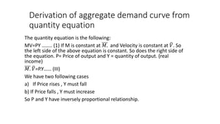
1. Derivation of aggregate demand curve from
quantity equation
The quantity equation is the following:
MV=PY …….. (1) If M is constant at 𝑀. and Velocity is constant at 𝑉. So
the left side of the above equation is constant. So does the right side of
the equation. P= Price of output and Y = quantity of output. (real
income)
𝑀. 𝑉=P.Y…… (III)
We have two following cases
a) If Price rises , Y must fall
b) If Price falls , Y must increase
So P and Y have inversely proportional relationship.

2. Q1: Derive the downward sloping AD curve
from quantity equation
• P P= Aggregate Price level.
• p1 A These two rectangles have same areas
• P2 B
• AD Curve is downward sloping
• 0 Y1 Y2 Y (Quantity of output demanded)

3. Q2. Why the AD curve is downward sloping?
• Economic interpretation:
• Logic-1: If Y Rises, demand for real money balance rises
𝑀
𝑃
𝑑
so the
supply of real money balance
𝑀
𝑃
rises. Since the M is constant at 𝑀.
Price level must fall. So we see as Y rises, Price level falls.
• Logic:2 If Y falls, demand for real money balance falls
𝑀
𝑃
𝑑
so the
supply of real money balance
𝑀
𝑃
falls. Since the M is constant at 𝑀.
Price level must rise. So we see as Y falls, Price level rises.

4. Q3.Under what circumstances downward sloping
AD curve shifts rightward and leftward?
• Rightward Shift: If Central Bank increases the money supply from 𝑀
to 𝑀1, such that 𝑀1> 𝑀.
• So 𝑀1. 𝑉 > 𝑀. 𝑉 …….(II) , 𝑀. 𝑉=P.Y…… (III)
• In equation (III) we have 𝑀1. 𝑉 = P.Y……. (IIIa) The right side of
equation (IIIa) is > right side of (III).
• For equation (IIIa), if P = fixed, Y rises
• if Y= Fixed , P rises
This is captured by rightward shift of the AD curve.

5. Graph of rightward shift of AD.
• P
• P// A B
• AD2
• AD1
• 0 Y1 Y2 Y (Quantity of output demanded)

6. Rightward shift of AD
• P
• Expansionary monetary policy leads to
• P2 B rightward shift of the AD curve.
• P1 A
• AD2
• AD1
• 0 Y// Y (Quantity of output demanded)

7. • leftward Shift: If Central Bank decreases the money supply from 𝑀 to
𝑀2, such that 𝑀2 < 𝑀.
• So 𝑀2. 𝑉 < 𝑀. 𝑉
• In equation (III) we have replaced and got the following:
• 𝑀2. 𝑉 = P.Y……. (IIIb) The right side of equation (IIIb) is < right side of
(III).
• For equation (IIIb), if P = fixed, Y Falls
• if Y= Fixed , P falls
This is captured by leftward shift of the AD curve.

8. Graph of leftward shift of AD
P
P// B A
AD1
AD2
0 Y2 Y1 Y

9. • P
• Contractionary monetary policy leads to leftward
• shift of AD.
• AD1
• AD2
• 0 Y// Y(Quantity of output demanded)

10. Time horizon in macroeconomics
• Long run and Short run:
• Price is rigid in short run . Movement of price is sluggish. There are
two reasons behind this a) labour supply is perfectly elastic b) the
menu cost faced by firm. (Prices are sticky)
• In the long-run the price is flexible . The movement of price is rapid.
• Short-run aggregate supply curve is horizontal and long run aggregate
supply curve is vertical.
• Behaviour of price is different across different time periods. Same
macroeconomic policy has differential impacts on output and price
in long run and short run.

11. Graphs of short run and long run aggregate
supply curve
Q4. What is the difference between SRAS
curve and LRAS curve?
SRAS: P P LRAS
P2
P// E
1
E
2 SRAS
P1
0 Y1 Y2 Y 0 𝑌 Y
0𝑌= Natural level of output. This is amount of output economy can produce
if it utilizes all its existing resources.( Land , skilled labour and capital: physical
and human)

12. Q5.Examine the effectiveness of monetary
policy in the short run and in the long run.
• Short run: If Central Bank increases the money supply the downward
sloping AD curve shifts towards the right. Equilibrium output rises but
the price level is unchanged. Expansionary monetary policy
• P is effective in SR to raise output.
• P// E
1
E
2
SRAS
• AD2
• AD1
• 0 Y1 Y2 Y(Quantity of output supplied and demanded)

13. • Short run: If Central Bank decreases the money supply the downward
sloping AD curve shifts towards the left. Equilibrium output falls but the
price level is unchanged. Contractionary monetary policy leads to
• P decrease in output level without having no
• P// E2 E1 SRAS change in price.
• AD1
• AD2
• 0 Y2 Y1 Y (Quantity of output demanded and supplied)

14. Effect of expansionary monetary policy in AD-
AS model.
• Long run: If Central Bank increases the money supply the downward
sloping AD curve shifts towards the right. Equilibrium output is constant at
natural level but the price level is increased.
• Draw the graph: P LRAS [ Monetary policy is not
• effective in raising output)
• P2 E2
• P1 E 1 AD2
• AD1
• 0 𝑌 Y

15. • Long run: If Central Bank decreases the money supply the downward
sloping AD curve shifts towards the left. Equilibrium output is
constant at natural level but the price level is declined.
• Draw the graph: P LRAS
• P1
• AD1
• P2 AD2
• 0 𝑌 Y

16. Q6. Verify the results in above question using
the quantity equation.
• M.V = P.Y ……….(I)
• Short run: We consider P to be constant at 𝑃. We also consider
Velocity to be constant at 𝑉. We substitute these in equation (1).
• M. 𝑉 =𝑃.Y …….. (Ia)
• We observe directly proportional relationship between M and Y. This
means if M rises by 2% , Y also rises by 2%.
• Graph also confirms the same result. In short run Money supply is
effective in raising output.

17. Result in the long run:
• M.V = P.Y ……….(I)
• Long run: We consider Y to be constant at 𝑌. We also consider
Velocity to be constant at 𝑉. We substitute these in equation (1).
• M. 𝑉 = P. 𝑌 …….. (Ib)
• We get directly proportional relationship between M and P.
• If M rises by 3% , Price level also rises by 3%, without having NO
impact on output. Output remains constant at natural level.