1. 1 2
3
4
5 6
16 dynamic 20
7 froot/leaf root depth
carbon increment
23 stress
8 relative 12 DBH bin 17 available based
height increment N 21 available mortality
18 water
9 dynamic Leaf C
leaf on/off
19 RUBP
10 13 22
dynamic
SLA
14
11 dynamic:
maint R
maint Q10
15 Stratum
QMD
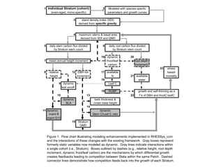
Figure 1. Flow chart illustrating modeling enhancements implemented in RHESSys_ccm
and the interactions of these changes with the existing framework. Gray boxes represent
formerly static variables now modeled as dynamic. Gray lines indicate interactions within
a single cohort (i.e., Stratum). Boxes outlined by dashes (e.g., relative height, root depth
increment, dynamic froot/leaf carbon) are the mechanisms by which differential growth
creates feedbacks leading to competition between Stata within the same Patch. Dashed
connector lines demonstrate how competition feeds back into the growth of each Stratum.
bark thickness &
crown base height
daily stem carbon flux divided daily root carbon flux divided
Stem C/Leaf C ratio
dynamic
F x of DBH and frootC:leafC
mean annual height increment
growth and self-thinning as a
by Stratum stem countby Stratum stem count
Individual Stratum (cohort)
(even-aged, mono-specific)
Modeled with species-specfic
parameters and growth curves
stand density index (SDI)
derived from specific gravity
maximum stems & basal area
derived from SDI and QMD

2. Preliminary results of RHESSys with an
embedded mechanistic fire model
Antoine Randolph
July 2012

3. Figure 2. physiographic regions. The initial letter is position (f-flatslope, l-lower slope, m-
midslope, r-ridge, u-upslope, v-valley), followed by aspect (N, NE, E, SE, S, SW, W, NW)

4. 0
0.05
0.1
0.15
0.2
0.25
0.3
3/15
3/17
3/19
3/21
3/23
3/25
3/27
3/29
3/31
date
equilibriummoisture
FWI-Ew FWI-Ed NFDRS - EMC
Figure 3. Comparison of equilibrium moisture content models: FFWI EMC and NFDRS
EMC for early March. Greatest differences occur from late fall through early Spring. The
least difference occurs at mid-summer (apprx. 5-8%)

5. coefficient exponent
code species name a b
acru Acer rubrum 0.83179 0.67012
acsa Acer saccharum 1.25681 0.55374
casp Carya spp. 3.61952 0.42127
cofl Cornus florida 1.84425 0.43455
fagr Fagus grandifolia 0.44877 0.68571
frsp Fraxinus 1.84999 0.66704
litu Liriodendron tulipifera 1.98836 0.63186
nysy Nyssa sylvatica 1.65387 0.6422
oxar Oxydendron arboreum 1.76025 0.66938
qual Quercus alba 1.60462 0.61482
quco Quercus coccinea 3.40407 0.42076
qupr Quercus prinus 3.66804 0.50767
quru Quercus rubra 2.62739 0.52988
quve Quercus velutina 2.95919 0.4809
saas Sassafras albidum 1.83967 0.67045
Table 1. Parameter values for fire stem necrosis allometic model

6. Coefficients Standard Error t Stat P-value
Intercept 2.7478 0.2442 11.2527 5.692E-21
FI 0.0094 0.0002 56.2425 1.31702E-93
ROS -54.5714 4.6559 -11.7210 3.82547E-22
twig diam -0.8876 0.0675 -13.1483 1.06438E-25
Species Mean Twig Diam (mm)
Acer rubrum 2.74
Acer saccharum 2.24
Carya spp. 4.74
Cornus florida 2.18
Fagus grandifolia 2.28
Fraxinus 4.45
Liriodendron tulipifera 4.44
Nyssa sylvatica 2.84
Oxydendron arboreum 2.26
Quercus alba 2.51
Quercus coccinea 3.45
Quercus prinus 2.82
Quercus rubra 3.2
Quercus velutina 3.58
Sassafras albidum 3.71
Table 2. Mean twig diameters and regression coefficients for calculation
of twig necrosis as a function of plume height of the flaming front, where
FI is fire line intensity in kW/m and ROS is rate of spread in meters/sec.

7. Table 3. Litter characteristics at simulation year 1965: L and F1 Layer biomass.
ACRU:no fire QUAL:no fire ACRU:10Yyr fire QUAL:10yr fire
Physiographic
Region
region area
(Ha)
LF1 biom.
(MT/Ha)
LF1 biom.
(MT/Ha)
LF1 biom.
(MT/Ha)
LF1 biom.
(MT/Ha)
Lowerslope-N 0.20 1.58 (0.58) 1.61 (0.06) 1.89 (0.99) 1.61 (0.07)
Lowerslope-SE 0.27 2.44 (0.38) 1.32 (0.06) 2.46 (0.51) 1.33 (0.05)
Midslope-E 0.46 1.98 (0.74) 1.23 (0.13) 1.98 (0.81) 1.23 (0.13)
Midslope-N 0.76 1.55 (0.58) 1.61 (0.09) 1.89 (1.02) 1.61 (0.11)
Midslope-S 0.34 1.74 (0.70) 1.19 (0.03) 1.85 (0.82) 1.20 (0.04)
Midslope-SE 1.79 1.92 (0.67) 0.89 (0.07) 2.00 (0.71) 0.89 (0.07)
Ridge-N 0.77 1.73 (0.16) 1.30 (0.27) 1.81 (0.32) 1.41 (0.26)
Ridge-S 0.57 1.24 (0.42) 1.15 (0.36) 1.34 (0.59) 1.13 (0.37)
Ridge-SE 0.84 1.41 (0.60) 0.98 (0.13) 1.43 (0.62) 0.97 (0.11)
Upslope-N 0.53 1.39 (0.36) 1.49 (0.17) 1.60 (0.68) 1.53 (0.08)
Upslope-S 0.69 1.50 (0.53) 1.03 (0.33) 1.56 (0.58) 1.00 (0.35)
Upslope-SE 2.07 1.76 (0.53) 0.97 (0.14) 1.88 (0.65) 0.96 (0.14)
Valley-N 0.36 1.55 (0.44) 1.59 (0.07) 1.83 (0.81) 1.59 (0.06)
Valley-SE 0.39 2.64 (0.36) 1.40 (0.07) 2.69 (0.54) 1.41 (0.06)

8. Table 4. Litter characteristics at simulation year 1965: L and F1 Layer depth.
ACRU:no fire QUAL:no fire ACRU:10Yyr fire QUAL:10yr fire
Physiographic
Region
region area
(Ha)
LF1_depth
(cm)
LF1_depth
(cm)
LF1_depth
(cm)
LF1_depth
(cm)
Lowerslope-N 0.20 2.98 (0.59) 2.99 (0.05) 3.24 (0.93) 2.98 (0.06)
Lowerslope-SE 0.27 3.75 (0.23) 2.70 (0.06) 3.77 (0.31) 2.70 (0.06)
Midslope-E 0.46 3.51 (0.43) 2.65 (0.10) 3.53 (0.44) 2.64 (0.10)
Midslope-N 0.76 2.95 (0.59) 2.99 (0.08) 3.23 (0.95) 2.99 (0.10)
Midslope-S 0.34 3.11 (0.71) 2.58 (0.02) 3.19 (0.79) 2.59 (0.02)
Midslope-SE 1.79 3.34 (0.56) 2.41 (0.11) 3.42 (0.57) 2.41 (0.11)
Ridge-N 0.77 3.38 (0.19) 2.70 (0.19) 3.36 (0.23) 2.78 (0.21)
Ridge-S 0.57 2.80 (0.58) 2.50 (0.36) 2.90 (0.68) 2.47 (0.39)
Ridge-SE 0.84 2.88 (0.65) 2.36 (0.09) 2.91 (0.67) 2.34 (0.07)
Upslope-N 0.53 2.94 (0.35) 2.84 (0.12) 3.14 (0.59) 2.86 (0.07)
Upslope-S 0.69 3.02 (0.53) 2.50 (0.27) 3.07 (0.56) 2.45 (0.30)
Upslope-SE 2.07 3.22 (0.45) 2.40 (0.12) 3.34 (0.51) 2.39 (0.12)
Valley-N 0.36 2.98 (0.48) 2.97 (0.07) 3.22 (0.80) 2.97 (0.05)
Valley-SE 0.39 3.88 (0.22) 2.78 (0.06) 3.92 (0.32) 2.79 (0.06)

9. Table 5. Litter characteristics at simulation year 1965: H Layer biomass and depth.
ACRU:no fire QUAL:no fire ACRU:no fire QUAL:no fire
Physiographic
Region
region area
(Ha)
H biom.
(MT/Ha)
H biom.
(MT/Ha)
H_depth
(cm)
H_depth
(cm)
Lowerslope-N 0.20 65.61 (2.97) 86.83 (1.78) 8.05 (0.36) 10.65 (0.22)
Lowerslope-SE 0.27 53.74 (2.35) 76.90 (2.37) 6.59 (0.29) 9.43 (0.29)
Midslope-E 0.46 54.67 (1.45) 63.77 (5.36) 6.70 (0.18) 7.82 (0.66)
Midslope-N 0.76 64.22 (2.92) 86.13 (2.31) 7.88 (0.36) 10.56 (0.28)
Midslope-S 0.34 49.63 (1.23) 68.97 (5.24) 6.09 (0.15) 8.46 (0.64)
Midslope-SE 1.79 49.10 (3.33) 55.49 (3.85) 6.02 (0.41) 6.80 (0.47)
Ridge-N 0.77 45.21 (7.91) 57.22 (6.31) 5.54 (0.97) 7.02 (0.77)
Ridge-S 0.57 48.10 (5.31) 53.94 (7.80) 5.90 (0.65) 6.62 (0.96)
Ridge-SE 0.84 46.60 (1.70) 53.94 (4.40) 5.72 (0.21) 6.61 (0.54)
Upslope-N 0.53 59.09 (4.26) 69.24 (13.73) 7.25 (0.52) 8.49 (1.68)
Upslope-S 0.69 49.32 (3.25) 54.45 (6.08) 6.05 (0.40) 6.68 (0.75)
Upslope-SE 2.07 47.63 (2.29) 57.24 (5.48) 5.84 (0.28) 7.02 (0.67)
Valley-N 0.36 64.32 (3.18) 85.94 (2.58) 7.89 (0.39) 10.54 (0.32)
Valley-SE 0.39 57.21 (1.51) 79.99 (2.30) 7.02 (0.19) 9.81 (0.28)

10. Spring Hillslope mean-daily litter moisture: qual
0
0.2
0.4
0.6
0.8
1
1.2 1
2
3
4
5
6
7
8
9
10
11
12
13
14
15
16
17
18
19
20
21
22
23
24
25
26
27
28
29
30
31
1
2
3
4
5
6
7
8
9
10
11
12
13
14
15
16
17
18
19
20
21
22
23
24
25
26
27
28
29
30
1
2
3
4
5
6
7
8
9
10
11
12
13
14
15
16
17
18
19
20
21
22
23
24
25
26
27
28
29
30
31
3 4 5
month/day
percentsaturation
L_sat% F1_sat% F2_sat% H_sat%
Figure 4. Mean daily litter moisture at the hillslope scale for spring of simulation year 1930

11. Fall Hillslope mean-daily litter moisture: qual
0
0.2
0.4
0.6
0.8
1
1.2 1
2
3
4
5
6
7
8
9
10
11
12
13
14
15
16
17
18
19
20
21
22
23
24
25
26
27
28
29
30
1
2
3
4
5
6
7
8
9
10
11
12
13
14
15
16
17
18
19
20
21
22
23
24
25
26
27
28
29
30
31
1
2
3
4
5
6
7
8
9
10
11
12
13
14
15
16
17
18
19
20
21
22
23
24
25
26
27
28
29
30
9 10 11
month/day
percentsaturation
L_sat% F1_sat% F2_sat% H_sat%
Figure 5. Mean daily litter moisture at the hillslope scale for fall of simulation year 1930.

12. Fall Patch mean-daily F2 litter moisture (Hillslope 1): qual
0
0.2
0.4
0.6
0.8
1
1.2
1
2
3
4
5
6
7
8
9
10
11
12
13
14
15
16
17
18
19
20
21
22
23
24
25
26
27
28
29
30
1
2
3
4
5
6
7
8
9
10
11
12
13
14
15
16
17
18
19
20
21
22
23
24
25
26
27
28
29
30
31
1
2
3
4
5
6
7
8
9
10
11
12
13
14
15
16
17
18
19
20
21
22
23
24
25
26
27
28
29
30
9 10 11
month/day
percentsaturation
Figure 6. A time series of F2 litter moisture for individual Patches in the same hillslope.

13. Fall Patch mean-daily H litter moisture (Hillslope 1): qual
0
0.2
0.4
0.6
0.8
1
1.2
1
2
3
4
5
6
7
8
9
10
11
12
13
14
15
16
17
18
19
20
21
22
23
24
25
26
27
28
29
30
1
2
3
4
5
6
7
8
9
10
11
12
13
14
15
16
17
18
19
20
21
22
23
24
25
26
27
28
29
30
31
1
2
3
4
5
6
7
8
9
10
11
12
13
14
15
16
17
18
19
20
21
22
23
24
25
26
27
28
29
30
9 10 11
month/day
percentsaturation
Figure 7. A time series of H litter moisture for individual Patches in the same hillslope.

14. October Patch mean-daily H litter moisture (Hillslope 1): qual
0.45
0.55
0.65
0.75
0.85
0.95
1 2 3 4 5 6 7 8 9 10 11 12 13 14 15 16 17 18 19 20 21 22 23 24 25 26 27 28 29 30 31
10
month/day
percentsaturation
Figure 8. Detail of H layer litter moisture for individual Patches in the same hillslope.

15. Table 6. Soil profile characteristics: mean mineralized N, rooting zone moisture and lower
soil profile moisture (simulation years 1930 to 1965). red maple (acru) and white oak (qual)
ACRU ACRU ACRU QUAL QUAL QUAL
Physiographic
Region
mineralized N
(kgN/m2)
rootzone
(sat. frac.)
lower profile
(sat. frac.)
mineralized N
(kgN/m2)
rootzone
(sat. frac.)
lower profile
(sat. frac.)
Lowerslope-N 0.059 (0.035) 0.173 (0.009) 0.345 (0.036) 0.084 (0.040) 0.168 (0.011) 0.331 (0.036)
Lowerslope-SE 0.068 (0.030) 0.174 (0.011) 0.340 (0.038) 0.088 (0.031) 0.166 (0.012) 0.339 (0.036)
Midslope-E 0.072 (0.030) 0.178 (0.007) 0.356 (0.043) 0.088 (0.027) 0.180 (0.011) 0.355 (0.044)
Midslope-N 0.060 (0.035) 0.170 (0.011) 0.341 (0.037) 0.085 (0.039) 0.165 (0.013) 0.328 (0.037)
Midslope-S 0.073 (0.023) 0.181 (0.007) 0.347 (0.047) 0.083 (0.030) 0.174 (0.010) 0.358 (0.041)
Midslope-SE 0.067 (0.025) 0.197 (0.029) 0.374 (0.042) 0.083 (0.025) 0.199 (0.029) 0.379 (0.039)
Ridge-N 0.074 (0.021) 0.214 (0.043) 0.372 (0.031) 0.078 (0.025) 0.208 (0.043) 0.365 (0.037)
Ridge-S 0.067 (0.021) 0.224 (0.034) 0.384 (0.038) 0.076 (0.023) 0.223 (0.033) 0.396 (0.039)
Ridge-SE 0.065 (0.017) 0.245 (0.009) 0.372 (0.034) 0.074 (0.020) 0.245 (0.011) 0.378 (0.037)
Upslope-N 0.061 (0.033) 0.179 (0.007) 0.355 (0.030) 0.087 (0.030) 0.178 (0.011) 0.358 (0.041)
Upslope-S 0.068 (0.024) 0.197 (0.029) 0.357 (0.041) 0.081 (0.025) 0.198 (0.029) 0.376 (0.043)
Upslope-SE 0.062 (0.022) 0.229 (0.029) 0.386 (0.044) 0.078 (0.023) 0.229 (0.031) 0.370 (0.038)
Valley-N 0.059 (0.035) 0.173 (0.009) 0.344 (0.032) 0.084 (0.039) 0.168 (0.011) 0.333 (0.038)
Valley-SE 0.068 (0.031) 0.163 (0.007) 0.322 (0.035) 0.087 (0.031) 0.156 (0.010) 0.322 (0.030)

16. Figure 9. Non-oak/hickory (noh) index for red maple without fire scenario. Increasingly negative values
indicate understory dominance by noh species. In this image, oak-hickory viability in the understory is limited
to red regions: ridge-N, lowerslope and midslope SE, and steep portions of lowerslope-N. Yellow equals areas
of moderate oak-hickory understory viability.

17. Figure 10. Non-oak/hickory index for an acru overstory with a 10yr fire return interval. Oak-hickory
understory viability expands in midsope SE, ridge S and SE and portions of ridge N. Success elsewhere on the
landscape is mixed. For example oak-hickory appears to lose ground in parts of lowerslope and midslope S.

18. Figure 11. Non-oak/hickory index for white oak without fire active. The area of understory viability
for oak-hickory species (red regions) is larger than the red maple overstory scenario, encompassing
much of upslope E, SE and S, midslope S and portions of upslope N and ridge N. Yellow areas reflect
regions where oak-hickory species are moderately competitive in the understory.

19. Figure 12. Non-oak/hickory index for qual with a 10yr fire return interval. The number of fires that
occurred in the qual simulation were limited. Therefore a relatively small portion of the landscape was
affected. The most significant change was an increase in oak-hickory understory success in midslope SE,
and an increase in areas of moderate understory success (yellow regions). Oak-hickory lost ground however
at ridge N and upslope N positions.

20. Table 7. Fire statistics: 10yr fire return interval beginning at year 1940. Burn frac is the percentage
of the region burned, ROS is rate of spread, FI is fire line intensity and girdle is the predicted depth to
which tissue necrosis would occur based on FI, ROS and residence time of the flaming front.
fire regime fire year Location
burn
frac.
ROS
(ft/min)
FI
(BTU/ft-sec)
flame ht.
(feet)
girdle depth
(mm)
post-grow 1941 Lowerslope-N 100% 9.3 (1.2) 200 (3.8) 4.5 (0.0) 2.89 (0.01)
post-grow 1941 Lowerslope-SE 100% 8.3 (0.7) 126 (16.4) 3.6 (0.2) 2.71 (0.07)
post-grow 1941 Midslope-E 100% 7.3 (0.7) 123 (12.2) 3.6 (0.2) 2.61 (0.04)
post-grow 1941 Midslope-N 100% 7.6 (0.5) 160 (10.9) 4.0 (0.1) 2.76 (0.03)
post-grow 1941 Midslope-S 98% 7.5 (0.7) 103 (7.1) 3.3 (0.1) 2.55 (0.04)
post-grow 1941 Midslope-SE 89% 7.3 (0.4) 101 (3.8) 3.3 (0.1) 2.56 (0.05)
post-grow 1941 Ridge-S 99% 7.2 (0.8) 99 (24.9) 3.2 (0.4) 2.40 (0.11)
post-grow 1941 Ridge-SE 73% 7.8 (0.2) 94 (4.9) 3.2 (0.1) 2.39 (0.05)
post-grow 1941 Upslope-N 99% 7.4 (0.6) 148 (17.7) 3.9 (0.2) 2.60 (0.15)
post-grow 1941 Upslope-S 97% 7.5 (0.9) 105 (16.0) 3.3 (0.2) 2.44 (0.06)
post-grow 1941 Upslope-SE 86% 8.0 (0.3) 101 (3.6) 3.3 (0.1) 2.45 (0.04)
post-grow 1941 Valley-N 100% 7.7 (1.0) 156 (1.0) 4.0 (0.0) 2.81 (0.13)
post-grow 1941 Valley-SE 98% 9.3 (0.5) 147 (8.0) 3.9 (0.1) 2.78 (0.03)
post-grow 1951 Lowerslope-N 100% 6.7 (0.9) 86 (19.3) 3.0 (0.3) 2.59 (0.13)
post-grow 1951 Valley-N 31% 6.6 (0.0) 81 (0.0) 3.0 (0.0) 2.56 (0.00)
post-grow 1954 Midslope-N 100% 10.6 (0.1) 146 (8.7) 3.9 (0.1) 2.64 (0.13)
post-grow 1954 Upslope-N 7% 9.3 (1.7) 123 (20.2) 3.6 (0.3) 2.57 (0.02)
post-grow 1954 Valley-N 69% 10.8 (0.0) 147 (0.0) 3.9 (0.0) 2.68 (0.00)
post-grow 1941 Lowerslope-N 100% 7.5 (1.2) 185 (56.6) 4.3 (0.6) 3.53 (0.11)
post-grow 1941 Midslope-N 59% 7.0 (0.0) 191 (0.0) 4.4 (0.0) 3.43 (0.00)
post-grow 1941 Valley-N 100% 6.6 (0.4) 157 (24.9) 4.0 (0.3) 3.51 (0.19)
post-grow 1946 Lowerslope-SE 100% 8.7 (0.7) 209 (24.2) 4.6 (0.2) 3.35 (0.10)
post-grow 1946 Midslope-S 56% 7.4 (0.1) 171 (1.1) 4.2 (0.0) 3.18 (0.02)
post-grow 1946 Valley-SE 98% 9.3 (0.7) 233 (12.5) 4.8 (0.1) 3.48 (0.03)
ACRU fire summary stats
QUAL fire summary stats

21. qual understory fire mortality
region acru acsa fagr litu nysy oxar casp qual quco qupr quru quve
Lowerslope-N 18.6 14.3 20.4 37.5 20.6 18.8 4.2 12.0 12.3 12.8 14.3 15.1
Lowerslope-SE 28.0 21.3 20.6 43.3 31.0 28.5 7.2 18.1 18.7 19.8 21.6 22.9
Midslope-E 0.0 0.0 0.0 0.0 0.0 0.0 0.0 0.0 0.0 0.0 0.0 0.0
Midslope-N 9.3 7.2 6.9 19.0 10.3 9.4 2.2 6.0 6.2 6.4 7.2 7.6
Midslope-S 18.7 14.3 13.7 23.1 20.8 19.0 5.0 12.2 12.6 13.1 14.4 15.3
Midslope-SE 0.0 0.0 0.0 0.0 0.0 0.0 0.0 0.0 0.0 0.0 0.0 0.0
Ridge-N 0.0 0.0 0.0 0.0 0.0 0.0 0.0 0.0 0.0 0.0 0.0 0.0
Ridge-S 0.0 0.0 0.0 0.0 0.0 0.0 0.0 0.0 0.0 0.0 0.0 0.0
Ridge-SE 0.0 0.0 0.0 0.0 0.0 0.0 0.0 0.0 0.0 0.0 0.0 0.0
Upslope-N 0.0 0.0 0.0 0.0 0.0 0.0 0.0 0.0 0.0 0.0 0.0 0.0
Upslope-S 0.0 0.0 0.0 0.0 0.0 0.0 0.0 0.0 0.0 0.0 0.0 0.0
Upslope-SE 0.0 0.0 0.0 0.0 0.0 0.0 0.0 0.0 0.0 0.0 0.0 0.0
Valley-N 18.6 14.3 27.1 37.5 20.6 18.8 4.2 11.9 12.4 21.0 14.3 15.1
Valley-SE 28.0 21.4 20.6 43.3 31.0 28.4 7.0 18.1 18.7 19.7 21.6 22.9
Table 8. Understory fire mortality for QUAL canopy scenario: values represent total stems girdled,
scaled to units of m2
of basal area lost per hectare. Zero indicates either that no fire occurred or that it
was not of sufficient intensity to girdle the species in the given physiographic region.

22. acru understory fire mortality
region acru acsa fagr litu nysy oxar casp qual quco qupr quru quve
Lowerslope-N 37.4 28.8 27.5 52.6 42.2 37.8 8.2 29.6 24.6 42.4 28.6 30.6
Lowerslope-SE 28.4 41.5 20.7 35.0 31.6 30.8 13.4 17.7 18.4 19.2 21.6 22.7
Midslope-E 28.4 41.7 20.7 34.7 31.6 30.3 11.8 18.0 28.4 19.2 21.6 32.8
Midslope-N 37.5 28.9 27.6 56.5 45.6 38.1 8.9 36.7 24.8 39.4 28.7 30.5
Midslope-S 28.6 31.7 20.8 35.3 31.8 31.8 14.4 17.7 18.5 20.0 22.1 22.8
Midslope-SE 28.7 41.7 20.7 35.3 32.2 31.7 14.2 17.8 18.7 20.0 22.1 22.7
Ridge-N 0.0 0.0 0.0 0.0 0.0 0.0 0.0 0.0 0.0 0.0 0.0 0.0
Ridge-S 28.9 22.4 39.5 35.3 32.3 31.4 13.0 18.1 18.7 20.5 22.4 22.9
Ridge-SE 29.0 22.5 39.2 35.4 32.5 32.2 14.7 17.7 18.8 20.8 22.6 22.7
Upslope-N 47.1 36.5 34.6 68.5 57.2 52.8 12.3 43.6 40.5 39.2 36.1 38.4
Upslope-S 38.3 29.1 27.6 47.0 52.8 41.8 17.5 23.9 24.9 27.3 29.7 30.4
Upslope-SE 28.9 22.5 20.8 35.4 32.5 32.2 14.4 17.8 19.1 20.6 22.6 22.8
Valley-N 37.4 28.8 34.8 54.7 43.8 37.9 8.5 30.3 24.7 26.0 28.6 30.6
Valley-SE 35.8 21.5 20.7 34.6 30.9 29.8 11.8 17.8 18.4 19.1 21.3 22.7
Table 9. Understory fire mortality for ACRU canopy scenario : values represent total stems girdled,
scaled to units of m2
of basal area lost per hectare. Zero indicates either that no fire occurred or that it
was not of sufficient intensity to girdle the species in the given physiographic region.

23. Figure 13. Basal area culled during the acru overstory scenario due to stem girdling
Basal areal loss: acru overstory scenario
0
100
200
300
400
500
600
acru acsa fagr litu nysy oxar casp qual quco qupr quru quve
species
m2
BA/Haculledbyfire
Valley-SE
Valley-N
Upslope-SE
Upslope-S
Upslope-N
Ridge-SE
Ridge-S
Ridge-N
Midslope-SE
Midslope-S
Midslope-N
Midslope-E
Lowerslope-SE
Lowerslope-N

24. Basal area loss: qual overstory scenario
0
50
100
150
200
250
acru acsa fagr litu nysy oxar casp qual quco qupr quru quve
species
m
2
BA/Haculledbyfire
Valley-SE
Valley-N
Upslope-SE
Upslope-S
Upslope-N
Ridge-SE
Ridge-S
Ridge-N
Midslope-SE
Midslope-S
Midslope-N
Midslope-E
Lowerslope-SE
Lowerslope-N
Figure 14. Basal area culled during the qual overstory scenario due to stem girdling

25. ACRU scenario understory species stem biomass change due to fire
region acru acsa fagr litu nysy oxar casp qual quco qupr quru quve
Lowerslope-N -609% -121% -158% 17% 64% 16% -13% -3% -39% 1% -229% -627%
Lowerslope-SE -92% -127% -74% -229% 28% -79% -10% 13% -12% 37% -46% 3%
Midslope-E -23% -16% -21% 34% 15% -48% -7% 7% 5% -221% -38% 39%
Midslope-N -157% -162% -720% -60% 46% 44% -13% 2% -197% 74% -318% -69%
Midslope-S -105% -62% -81% -2225% -528% -553% -33% -257% -162% 7% -105% -463%
Midslope-SE -802% -1013% -63% -187% 7% -955% -496% -11% -130% -11% -99% -934%
Ridge-S -345% -410% -48% -2198% -218% -376% -308% -411% -221% -1988% -160% -324%
Ridge-SE -1253% -194% -92% -157% 0% -608% -141% -12% -432% -253% -286% -201%
Upslope-N -128% -371% -664% -367% 31% 28% -12% -4% -166% 54% -259% -137%
Upslope-S -170% -183% -53% -221% -17% -318% -474% -26% -181% -1173% -83% -75%
Upslope-SE -390% -176% -85% -110% -122% -229% -220% -17% -353% -240% -226% -50%
Valley-N -271% -163% -278% -2118% 72% 50% -11% 5% -58% 43% -201% -153%
Valley-SE -11% -91% -23% -22% 76% -62% -13% -3571% 37% -229% -412% 11%
QUAL scenario understory species stem biomass change due to fire
region acru acsa fagr litu nysy oxar casp qual quco qupr quru quve
Lowerslope-N 17% -360% 37% 1% 52% 19% 0% 15% -94% 17% -131% 14%
Lowerslope-SE -12% -3% -1343% 8% -94% 16% -3% 32% -83% 18% -212% -327%
Midslope-N 14% 20% -38% 2% 27% 20% -1% 17% -299% 19% -122% 25%
Midslope-S -154% -160% -204% 13% -487% -479% -3% 12% -233% 11% -215% -537%
Valley-N 16% 6% 51% 1% 22% 19% 0% 19% 4% 18% -132% 22%
Valley-SE -115% -1284% -713% 6% 49% 14% -3% 20% -173% -564% -150% -358%
Table 10. Change in understory stem biomass at year 1965 between simulations without fire active and
simulations with a 10yr fire return interval. Differences between qual and acru canopy series reflect
interactions between topographic position, fuel loading, fuel moisture, fire frequency and species
tolerances to fire.

26. Change in stem biomass between fire and non-fire
simulations (acru overstory): Midslope N
-800%
-700%
-600%
-500%
-400%
-300%
-200%
-100%
0%
100%
200%
acru acsa fagr litu nysy oxar casp qual quco qupr quru quve
percentchange
Total
Figure 15. Qupr, nysy, oxar and qual gain stem biomass at the Midslope N position when a 10yr fire
return interval is implemented.

27. Change in stem biomass between fire and non-fire
simulations (acru overstory): Midslope S
-2500%
-2000%
-1500%
-1000%
-500%
0%
500%
acru acsa fagr litu nysy oxar casp qual quco qupr quru quve
percentchange
Total
Figure 16. At the Midslope S position, all species lose stem biomass relative to the non-fire scenario
when a 10yr fire return interval is implemented. But the degree of loss varies by orders of magnitude.