1. Addressing the Affordability of Housing in
England Using a Residual Income Approach
Thomas Markovitch
Student ID: 1204381
RAE Tutor: Dr. Dean Garratt
Word Count: 4978 words
ABSTRACT
The UK is in a housing crisis, with both declining homeownership and
housing affordability since 2002. The conventional measure of housing
affordability is an earnings to house price ratio, measured at the lower quartile or
median. This study builds upon previous research by developing a new measure;
Real Residual Income (RRI), and estimates the causes of declining housing
affordability in England, from 1996 to 2012. The primary finding is that a
commitment to substantial year on year housing construction is necessary to
mitigate housing affordability decline. The paper also encourages future use of RRI
measurement and an exploration into the effects of tenure type.
I take this opportunity to thank Dr. Dean Garratt for his guidance during the academic year,
insight into the topic, and invaluable reassurance throughout the challenges of the project.

2. Contents
1 Introduction………………………………………………………………………………… 1
2 Literature Review………………………………………………………………………… 1
3 Data
3.1 Defining Entities……………………………………………………………………………… 3
3.2 Real Residual Income………………………………………………………………………… 4
3.3 Supply-Side Variables…………………………………………………………………………6
3.4 Demand-Side Variables……………………………………………………………………… 7
4 Methodology
4.1 Deriving Real Residual Income……………………………………………………………….9
4.2 Hypotheses…………………………………………………………………………………… 10
4.3 Model………………………………………………………………………………………… 10
5 Results………………………………………………………………………………………….11
6 Discussion
6.1 Limitations and Extensions……………………………………………………………………14
6.2 Conclusion……………………………………………………………………………………. 14
7 References……………………………………………………………………………………. 15
8 Appendix
8.1 Appendix A: Help to Buy …………………………………………………………………… 19
8.2 Appendix B: NUTS 1 Regional Grouping ……………………………………………………19
8.3 Appendix C: FRS Group Sizes……………………………………………………………… 20
8.4 Appendix D: Shelter Poverty Affordability Scale…………………………………………… 20
8.5 Appendix E: Additional RRI Findings……………………………………………………… 22
8.6 Appendix F: Variation of Mean Adults per Household ……………………………………… 22
8.7 Appendix G: Additional Population Variables……………………………………………… 23
8.8 Appendix H: Additional Variables…………………………………………………………… 24
8.9 Appendix I: RRI Composition……………………………………………………………….. 27
8.10 Appendix J: Data Mining Process……………………………………………………………28

3. 1 Introduction
In 1914, 10% of Britons were homeowners with 89% privately renting and less than 1%1
publicly renting (Mullins and Murie, 2006). Increasing homeownership spanned nine decades ,2
peaking at 69.52% in 2002, before falling to 63.85% by 2012, (DCLG, 2014). However, housing3
affordability was in decline for some time prior to 2002. Barker (2004, p. 123) discovered that “In
2002, only 37 per cent of new households could afford to buy a property, compared to 46 per cent in
the late 1980s”. Poon and Garratt (2012) illustrate this decline with house price, earnings and inflation
data from 1969-2012; while real household income increased by a factor of 2.75, real house prices
increased by a factor of 3.92. From a European prospective, this was due to soaring house prices,
rather than slow earnings growth. During 1971-2001, the UK’s real average house price increased at
2.4% per annum (pa.); 1.3 percentage points (pp.) higher than the European average (Mean, 2011).
It is clear that potential first time buyers, or ‘outsiders’ (Meen, 2013), are losing access to the
housing market. However, the fall in affordability, rather than plateau, shows that existing owners, or
‘insiders’, are also exiting . Thus, housing affordability is the dual problem of tougher attainability,4
and tougher sustainability. This is of particular concern in England, where half of owner occupiers are
mortgage holders (ONS, 2013c). In 2013-14, the balance tipped, with outright owners exceeding the
number of mortgage holders for the first time in three decades (DCLG, 2015). To investigate the
causes behind the decline in housing affordability in England, this paper proposes and develops an
alternative measure; Real Residual Income (RRI), and estimates the model over 1996-2012.
2 Literature Review
Declining affordability has widened the economic gap between insiders, (especially those
with outright ownership), and outsiders, with a bias in favour of older generations. In 2012, only 17%
of 18-24 year olds were homeowners (Pannell, 2012). In 2013, George Osborne, Chancellor of the
Exchequer, proposed the ‘Help to Buy’ scheme, (Appendix A), to counteract this issue (BBC, 2013).
However, it was a housing demand solution to an inherently housing supply problem.
In 2003, the British Government commissioned the ‘Review of Housing Supply’, to analyse
the “issues underlying the lack of supply and responsiveness of housing in the UK” (Barker, 2004, p.
3). In 2004, Economist Kate Barker, member of the Monetary Policy Committee, outlined the
following motivations for leading the review: (1) weak housing supply hinders economic growth,
causes macroeconomic instability, and reduces flexibility within the labour market; (2) housing
security is necessary for households to financially plan for their futures, and access key services
nationally, and within their local communities; (3) lastly, and most poignantly, Barker explains:
Includes housing associations.1
Brief exception to the trend during and caused by the Second World War.2
Calculated by owner occupied dwelling stock over total dwelling stock.3
Even if population growth contributed only to a non-ownership group, it still wouldn’t account for the 5.67pp.4
decline.
! /!1 28

4. Barker’s final report recommended the Government establish a “market affordability goal”,
and that each region “set its own target to improve market affordability”, to be “consistent with the
Government target” (Barker, 2004, p. 131). This made the discussion of housing affordability
particularly prominent throughout the late 2000s. In response to Barker’s recommendations, the
Department of Communities and Local Government (DCLG) commissioned the construction of the
‘Affordability Model’, developed between 2005 and 2010 (Mean, 2011). The model has since been
used as a basis for English housing affordability research and policy analysis. Like most previous
affordability research, it adopts a house price to earnings ratio as its measure of housing affordability.
Sophisticated measures of housing affordability began to emerge in the UK during the early
1990s (Stone, 2006). However, in the US, “poverty and urban problems” initiated the discussion of
appropriate housing affordability measurement from the late 1960s (Stone, 2006, p. 457). One of the
earliest measures was the ratio of median house prices to median earnings. This method was soon
identified as flawed by inadequately representing lower income households, and disregarding the
effects of interest rates and mortgage repayments (Jones et al., 2010). The ratio fails for lower income
households because an ‘acceptable’ ratio results in a level of non-housing income that is significantly
less than required to sustain an acceptable standard of living (Grigsby and Rosenberg, 1975).
The ratio’s usefulness also diminishes the more heterogeneous the income of the population.
Studies of the 2000s refine the approach, addressing such problems, for example, constructing the
ratio at 25% quartiles. Wilcox and Bramley (2010) criticise this solution, affirming that 25% quartiles
are arbitrary and familiarised among literature with little justification . Dolbeare (1966) offered one of5
the first compelling arguments against the ratio approach by proposing the use of residual income.
Residual income is defined: “the amount of money left after housing costs have been met that is
crucial in determining whether the costs of housing are really affordable” (Brownill et. al, 1990, p.49).
Residual income is more logical in construction, but is nonetheless faced with significant
resistance in adoption. Firstly, the ratio approach is widely recycled in housing affordability research
and considered the conventional method. Secondly, residual income is difficult to operationalise; its
generation requires comprehensive household surveys with individual specific information, rather
than macroeconomic time series. Furthermore, survey based methods face the criticism that a result
“is not universal; it is socially grounded in space and time” (Stone, 2006, p.459).
However, cross-sectional housing affordability research is not uncommon. For example,
Bourassa (1996) explores the household specific factors effecting affordability in Australian cities.
Stone (2006), an advocate for residual income, derives the variable by creating a ‘market basket’ of all
non-housing necessities, to determine the amount a household can spend on housing, once the
necessity market basket is paid for. To benefit from both the residual income approach, and time series
variables, this paper aggregates multiple household surveys, to form real residual income over time.
Wilcox and Bramley prefer the midpoint between the 10% decile and 25% quartile.5
! /!2 28
For many people, housing has become increasingly unaffordable
over time. The aspiration for homeownership is as strong as ever, yet the
reality is that for many this aspiration will remain unfulfilled unless the
trend in real house prices is reduced. This brings potential for an ever
widening social and economic divide between those able to access market
housing and those kept out. (Barker, 2004, p. 1)

5. 3 Data
3.1 Defining Entities
A prerequisite in forming the residual income model is to define entities, such as region and
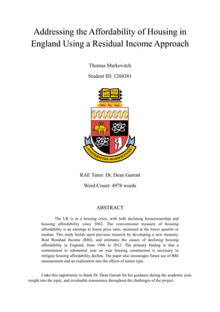
tenure, and to determine the time period over which the model can be estimated. Regional effects of
housing affordability follow a similar pattern through time, but with different magnitudes and
volatilities, as shown by Figure 1 (Nationwide, 2014). By the fourth quarter of 2014, London’s ratio
exceeded all other regions by a factor of 1.46 to 2.65, with additional volatility of 9.94% to 36.80%6
over the period. Further support of specifying regional effects is the heterogeneous housing policy
between regions, and historical factors influencing regional differences, such as economic sector
proportions, wealth distribution and demography.
Previous affordability models, including the Affordability Model and Long-run Model of
Housing Affordability (Meen, 2011), divide England into nine regions. This study uses the same
approach. Appendix B contains a thorough justification, methodology and map outlining the regional
boundaries. Figure 2 plots the housing affordability ratio, measured at lower quartiles, by these nine
regions, during 1997-2011, which draw much the same conclusions as Figure 1 (Parliament, 2012).
Dividing by region determines the time horizon of the model, due to annual regional data available
from 1996-2012. To reduce repetition, this paper adopts abbreviations for regions by the bracketed
letters in Figure 2. Furthermore, all variables and diagrams after Figure 2 are measured annually, from
1996-2012.
Only two data services measure variables by region and tenure; the Family Resources Survey
(FRS) and English Housing Survey (EHS). The FRS was selected due to its age, containing seventeen
years of data, rather than six. The FRS is an annual UK-wide cross-sectional survey, containing 25
Volatility is measured by the coefficient of variation (throughout this study) to account for magnitude effects.6
! /!3 28
1
2
3
4
5
6
7
8
9
10
83 85 87 89 91 93 95 97 99 01 03 05 07 09 11 13
Ratio(mean)
Year
Figure 1: Quarterly Regional Housing Affordability Ratios, 1983 - 2014
Northern
Yorkshire and the Humber
North West
East Midlands
West Midlands
East Anglia
Outer South East
Outer Met
London
South West

6. datasets with more than 2,000 variables. During 1996-2012, the FRS’s distinguish between six types
of tenure ; rent from the council, housing association or privately (furnished and unfurnished) and7
owner occupied, with or without a mortgage.
A potential problem of grouping by region and tenure is generating a small sample size per
group. However, during 1996-2012, the smallest annual survey contained 20,196 UK households ,8
consisting of 11,213 children and 35,207 adults. Once privately furnished and unfurnished renters
were grouped together , the median group size contained 316 households. This is assumed sufficiently9
large to be representative of the population, with the tolerance of error discussed in Section 3.2.
Appendix C contains further group size statistics. Henceforth, renter tenure types are abbreviated to
‘Council’, ‘HA’ and ‘Private’, and homeowners to ‘Outright’ and ‘Mortgage’.
3.2 Real Residual Income (RRI)
RRI is derived in Section 4.1. Once computed by region and tenure, median (with a 2.5%
upper confidence interval ) and mean household nominal residual income (NRI) are compared in10
Figure 3 . The mean values often exceed the upper confidence interval of the median calculations.11
Thus, similarly to the ratio approach, percentiles are preferred in the calculation of residual income
because of the upward skewness caused by outliers (very high income households). To illustrate the
two-way tolerance of error, and real transformation in comparison to Figure 3, Figure 4 plots median
household RRI with a 5% confidence interval.
‘Part own, part rent’ was an additional category in 1996, containing 64 observations (0.291% of the 19967
sample). By including 1996 data, the overall dataset increased by 6.25%. It is assumed that removing the 64
observations was an insignificant random loss, not systematically related to any regressors.
Consisting of 14,365 English households, once removing Wales, Scotland and Northern Ireland.8
As the furnished category alone had a small sample size. In the 2012/13 survey, it only contained 11 - 409
observations per region, except for London with 75 observations.
Using a conservative binomial exact confidence interval (used throughout the paper) which makes no10
assumptions about the underlying distribution of household residual income.
North East was chosen as it was coded region ‘1’ in dataset, but all regions show similar results.11
! /!4 28
2
3
4
5
6
7
8
9
10
97 98 99 00 01 02 03 04 05 06 07 08 09 10 11
Ratio(lowerquartile)
Year
Figure 2: Regional Housing Affordability Ratios, 1997 - 2011
North East (NE)
North West (NW)
Yorkshire and the Humber (YH)
East Midlands (EM)
West Midlands (WM)
East of England (EE)
London (LO)
South East (SE)
South West (SW)
England

7. Unexpectedly, Figure 4 shows that measuring housing affordability by RRI, doesn’t produce a
declining trend. However, lower quartile RRI results expose that a substantial proportion of renters,
across all regions, have a standard of living below an ‘acceptable level’. This discrepancy is
calculated by applying Stone’s (2006) ‘Shelter Poverty Affordability Scale’, discussed in detail in
Appendix D. This finding supports that increasing RRI should remain a priority to policy makers.
A second unanticipated result is that mortgage holders have significantly higher RRI than
outright owners. This is likely explained by the higher proportion of retirement aged people owning
their homes outright, relative to younger people. For example, in the 2012 FRS, 66.95% of outright
owner households contained at least one person of retirement age, compared to just 7.31% of
mortgage holder households. As people of retirement age tend to work less, outright owners’ weekly
median net income is lower, (£240.72 less in the North East, during 1996-2012), which doesn’t fully
compensate for their housing cost savings (£49.85).
Further RRI findings are discussed in Appendix E.
! /!5 28
100
200
300
400
500
600
700
96 97 98 99 00 01 02 03 04 05 06 07 08 09 10 11 12
NRI(£/week)
Year
Figure 3: NE NRI by Tenure
Council, mean
Council, median
Council, upper CI
HA, mean
HA, median
HA, upper CI
Private, mean
Private, median
Private, upper CI
Outright, mean
Outright, median
Outright, upper CI
Mortgage, mean
Mortgage, median
Mortgage, upper CI
100
200
300
400
500
600
700
96 97 98 99 00 01 02 03 04 05 06 07 08 09 10 11 12
RRI(£/week)
Year
Figure 4: NE RRI by Tenure, (2012 Prices)
Council, lower CI
Council, median
Council, upper CI
HA, lower CI
HA, median
HA, upper CI
Private, lower CI
Private, median
Private, upper CI
Outright, lower CI
Outright, median
Outright, upper CI
Mortgage, lower CI
Mortgage, median
Mortgage, upper CI

8. 3.3 Supply-Side Variables
Two supply-side variables are included in the final model; homeownership rate and housing
stock, and both are unavailable by tenure (DCLG, 2012 and 2014). Since 2012, homeownership and
housing stock were no longer collected at the regional level, so the 2012 observations are estimated
from the change in the English rate . This approximation seems appropriate as all regions follow a12
similar trend (and thereby to England), as shown in Figures 5 and 6. Aggregately, the estimation is
correct because the combined weighted changes equal the English change.
Figure 5 shows that London’s homeownership is significantly lower than in other regions.
This is mostly explained by its constantly higher house price increases and population growth (by
both natural increase and net migration). The housing stock trends of Figure 6 appear linear, but are
more revealing when scaled by their annual regional populations, as presented in Figure 7. Except for
London, the housing stock per 1,000 residents, increased up to and past the 2002 homeownership
percentage peak. The trend has only recently appeared to revert into decline, importantly exposing
For example, as English housing stock increased by 0.588%, regions were assigned a 0.588% increase.12
! /!6 28
48
52
56
60
64
68
72
76
80
96 97 98 99 00 01 02 03 04 05 06 07 08 09 10 11 12
HomeowenrshipRate(%)
Year
Figure 5: Regional and National Homeownership Rate
NE
NW
YH
EM
WM
EE
LO
SE
SW
England
1,000
1,500
2,000
2,500
3,000
3,500
4,000
96 97 98 99 00 01 02 03 04 05 06 07 08 09 10 11 12
Stock(000s)
Year
Figure 6: Regional Housing Stock
NE
NW
YH
EM
WM
EE
LO
SE
SW

9. that housing stock is not only determinant driving homeownership decline. London’s housing stock is
a completely separate case; during 1996-2012, homes became increasingly competitive at the mean
rate of 1.86 fewer stock per 1,000 residents pa..
3.4 Demand-Side Variables
The demand-side variables of the model include the mean number of adults per household
(FRS, 1995-2012); the unemployment rate (ONS, 2015); and a variety of population statistics (ONS,
1998a/b-2014a/b and 2014c). The mean number of adults is measured by region and tenure. The
unemployment rate and population variables are only measured by region. Variation within the mean
number of adults is primarily due to regional differences (59.5%) which are explored in Appendix F.13
Figure 8 plots the unemployment rate which varies in magnitude from region to region, but has
changed much the same in all regions, (a positive parabola between the early 1990s recession and the
2007-08 financial crisis).
Time and tenure account for 25.6% and 14.9% respectively.13
! /!7 28
400
405
410
415
420
425
430
435
440
445
450
455
96 97 98 99 00 01 02 03 04 05 06 07 08 09 10 11 12
Stockper1,000Residents
Year
Figure 7: Regional Housing Stock per 1,000 Residents
NE
NW
YH
EM
WM
EE
LO
SE
SW
3
4
5
6
7
8
9
10
11
12
96 97 98 99 00 01 02 03 04 05 06 07 08 09 10 11 12
UnemploymentRate(%)
Year
Figure 8: Regional Unemployment Rate
NE
NW
YH
EM
WM
EE
LO
SE
SW

10. The model includes three population statistics; births, deaths and net migration, with subsets
and supersets discussed in Appendix G. Emigration and immigration aren’t included separately
because of their high correlation (0.9527), which would induce multicollinearity in estimation.
Regional patterns are easily identified after scaling by annual population. Figure 9 shows that
natural increase (births minus deaths) ranges between ≈-1 to ≈4 people per 1,000 residents, per region,
except for London. The capital’s differences relate to its age profile. In 2012, it proportionately had
36% less retirement age inhabitants, and a median age (34) six years younger than the UK average
(ONS, 2013d). Young migrants play a significant contributing factor with Figure 10 displaying
regional migration per 1,000 residents pa.. London’s immigration was so high during 1996-2005, that
its net migration rate exceeded the average immigration rate of the other regions.
Appendix H discusses some additional variables commonly used in housing affordability
research and the reasons for their exclusion in this study’s model.
! /!8 28
-2
0
2
4
6
8
10
12
96 97 98 99 00 01 02 03 04 05 06 07 08 09 10 11 12
NaturalIncreaseper1,000Residents
Year
Figure 9: Regional Natural Increase per 1,000 Residents
NE
NW
YH
EM
WM
EE
LO
SE
SW
-2
0
2
4
6
8
10
12
14
16
96 97 98 99 00 01 02 03 04 05 06 07 08 09 10 11 12
Migrantsper1000Resdients
Year
Figure 10: Regional Migration per 1,000 Residents
NE Net
NW Net
YH Net
EM Net
WM Net
EE Net
SE Net
SW Net
Regions exc. London Mean Immigration
Regions exc. London Mean Emigration
LO Net

11. 4 Methodology
4.1 Deriving Real Residual Income (RRI)
There is no widely accepted mathematical derivation of residual income. Stone (2006) uses
weekly disposable household income minus weekly shelter cost . Disposable income is used to best14
represent the amount of money households have to spend on goods and services, outside of housing.
This paper uses the same approach, but different terminology (net income and housing cost), to be
consistent with the FRS. Appendix I contains a comprehensive FRS definition of these variables.
The desired unit of measurement was at the household level, as this reduces irrelevant net
income fluctuation from households containing working and non-working adults. It also prevents
otherwise necessary systematic division of housing costs amongst household members. The FRS15
does not measure net income at the household level, but provides identification numbers (IDs) to all
children, adults and households in three datasets. Thus, it was possible to construct residual income
per household, by region and tenure for each survey year, by Equation 1.
(1)
The equation aggregates children and adult net income into their respective households and
subtracts the housing cost of each household. The household index was then removed by finding the
mean (Equation 2) or median (Equation 3). Finally, substantial data mining was conducted to obtain16
real data from Equations 2 & 3, as outlined in Appendix J.
(2)
(3)
Housing benefit and council tax are only included in shelter cost (to not be counted twice).14
The process would need to take into account several factors such as relative net income in the household and15
likelihood of being the payer of the housing cost.
Lower quartiles were also found by adjusting the median equation’s ‘(n+1)/2’ to ‘(n+1)/4’.16
! /!9 28
RRIhirt ≡ NIahirt
a=1
p
∑ + NIchirt
c=1
q
∑ − HChirt , h = 1,...,n, a = 1,..., p & c = 1,...,q
where: RRI = real residual income NI = net income HC = housing cost
i = tenure r = region t = year
a = adult c = child h = household
p = total adults q = total children n = total households
RRIirt
mean
=
1
n
NIahirt + HIchirt
c=1
q
∑
a=1
p
∑
⎛
⎝⎜
⎞
⎠⎟ − HChirt
⎡
⎣
⎢
⎤
⎦
⎥
h=1
n
∑
RRIirt
median
=
n +1
2
term from: NIahirt + HIchirt
c=1
q
∑
a=1
p
∑ − HChirt

12. 4.2 Hypotheses
Regional effects and housing supply are widely confirmed determinants of housing
affordability. Thus, hypothesis 1 & 2 are partial validity tests of RRI measurement. Hypothesis 3 tests
the less discussed demand-side impacts, and hypothesis 4 assesses London effects. Finally, hypothesis
5 tests the strength of the commonly reported primary determinant of housing affordability.
Hypothesis 1: H0: Regional effects have no effect on RRI.
Hypothesis 2: H0: Supply-side variables have no effect on RRI.
Hypothesis 3: H0: Demand-side variables have no effect on RRI.
Hypothesis 4: H0: No supply-side or demand-side variables have an additional effect for
London on RRI, relative to other regions.
Hypothesis 5: H0: RRI is inelastic with respect to a change in the housing stock.
4.3 Model
Although Section 3 provides evidence of tenure differentiation, too few variables are
available by tenure to include tenure effects, as the coefficients on the tenure dummy variables would
be highly biased. The bias is caused by the omission of tenure effects from the variables not measured
by tenure, but which do vary by tenure, and effect RRI, such as housing stock, unemployment and
demography. Thus, all FRS series were re-calculated without tenure. The implications are discussed in
Section 6.1. Equations (1) - (3) remain the same, except for the omission of the tenure (i) index.
If time invariant regional effects (unobserved heterogeneity) impact independent variables,
they must be removed to prevent biased estimates. There are several examples of this problem, such
as London's status as a global financial services centre, influencing employment and population
variables, or the South East’s better weather, attracting a disproportionate number of retirement aged
people, impacting the birth and death rate. Pooled OLS estimation contains heterogeneity bias by
failing to remove the unobserved heterogeneity, ar. Random Effects is invalid by construction
(requiring zero correlation between ar and RRI regressors, x1rt,…, xkrt).
Both fixed effects (FE) and first differencing (FD) remove unobserved heterogeneity.
However, a problem with both methods that they cannot include time invariant variables, or variables
which do not vary by entity. While the coefficient estimates remain unbiased, the impact of such
variables (such as credit restrictions) cannot be estimated. Wooldridge (2013) states that under usual
panel data assumptions, the decision between FE and FD, ultimately depends on the relative
efficiencies of the estimators. FD is preferred when the observed factors which change over time are
serially correlated. As serial correlation is detected in the FD idiosyncratic errors, Δεrt (p = 0.0004),
the FD model is not appropriate. Wooldridge (2013) explains it is difficult to test for serial correlation
for FE, so insignificant serial correlation in the time demeaned idiosyncratic errors is assumed. After
including London interaction terms for variables which are noticeably different in London to other
regions, the FE model is derived from pooled OLS (Regression 4), giving Regression 7.17
Technically, the unobserved heterogeneity includes an intercept and Stata estimates FE by assuming: 17
but the outcome is the same. For interpretation purposes, net migration is measured in 000s and the
homeownership and unemployment rate level variables are measured from 0 to 100 (e.g. 65 refers to 65%).
! /!10 28
ar
r=1
9
∑ = 0

13. (4)
(5)
(6)
(7)
5 Results
Hypothesis 1 is test by the dummy regression model given by Regression 8:18
(8)
Hypothesis 1:
Result: Reject H0 at the 1% significance level , thus rejecting that regional effects have no effect on19
RRI. All other hypotheses are test by Regression 7 with estimation results given in Table 1.
Produces identical coefficients to usual FE, but includes regional dummy variables for testing.18
Independent of the robustness decision of the standard errors.19
! /!11 28
ln RRIrt( )= β1x1rt +...+ β7x7rt + δtdt
t=2
17
∑ + Lr bj xjrt
j=1
5
∑ + ar + εrt
ln RRIr( )= β1 x1r +...+ β7 x7r +
1
17
δt
t=2
17
∑ + Lr bj xjr
j=1
5
∑ + ar + εr
⇒ ln RRIrt( )− ln RRIr( )= β1 x1rt − x1r( )+...+ β7 x7rt − x7r( )+ δt dt −
1
17
⎛
⎝⎜
⎞
⎠⎟
t=2
17
∑
+ Lr bj xjrt − xjr( )j=1
5
∑ + ar − ar
removal of the
unobserved
heterogeneity
!"#
+ εrt − εr
= ln R!!RIrt( )= β1!!x1rt +...+ β7!!x7rt + δt
!!dt
t=2
17
∑ + Lr bj !!xjrt
j=1
5
∑ + !!εrt
where : r = region t = year
x1 = ln housing stock( ) x2 = net migration
x3 = ln births( ) x4 = ln deaths( )
x5 = homeownership rate x6 = ln adults per household( )
x7 = unemployment rate L = London dummy variable
dt
t=2
17
∑ = set of time annual dummy variables ar = unobserved heterogeneity,
Lt xjrt
j=1
6
∑ = set of London interaction variables εrt = idiosyncratic error
− = meaned variables ..= demeaned variables
ln RRIrt( )= β1x1rt +...+ β7x7rt + δtdt
t=2
17
∑ + Lr bj xjrt
j=1
5
∑ + γ rλr
r=2
9
∑ + εrt
H0 :γ 2 = ...= γ 9 = 0
H1 :γ 2 = ...= γ 9 ≠ 0

14. Table 1: Fixed Effects Output
* significant at p < 0.01; ** at p < 0.05; and *** at p < 0.01
Hypothesis 2 and 3 can be written as follows:
Hypothesis 2:
Hypothesis 3:
Result: Reject H0 from hypothesis 2 (3) at the 1% (5%) significance level, thus rejecting that20
supply-side (demand-side) variables have no effect on RRI. The highly significant results from
hypothesis 1 & 2 are consistent with the ratio approach, providing evidence that RRI is an
appropriate measure of housing affordability.
Moreover, Table 1 shows that four variables are statistically and economically significant.
Succinctly, a 1% increase in the housing stock, mean adults per household, births and deaths increase
RRI by 1.304%, 1.114%, -0.536% and -0.474% respectively. While the directions for the housing
stock and mean adults per household variables are obvious, the birth and death rate effects are less so.
The negative birth rate effect is likely due to a parent(s) reducing employment, (and thereby reducing
household net income), to look after the newborn. The negative death rate effect essentially works in
the direct opposite manner to the mean adults per household variable; a death causes an immediate
loss to household net income, while housing costs remain unchanged.
Any single variable test rejecting the null hypotheses is sufficient, for instance H0: β4 = 0, H1: β4 ≠ 0 for20
hypothesis 3, or a supply or demand multivariable test, as the hypotheses were not variable/combination
specific.
! /!12 28
Variable Coefficient Standard Error T-statistic
Housing stock 1.304*** 0.444 2.94
Net migration 0.000 0.000 1.10
Births -0.536** 0.221 -2.42
Deaths -0.474** 0.218 -2.18
Homeownership 0.011*** 0.004 2.70
Adults per household 1.144*** 0.158 7.24
Unemployment -0.012** 0.005 -2.48
London*Housing stock 1.613 1.981 0.81
London*Net migration 0.000 0.001 -0.35
London*Births -0.451 0.358 -1.26
London*Deaths -0.099 0.452 -0.22
London*Homeownership 0.005 0.010 0.53
H0 :β1 = 0
H1 :β1 ≠ 0
H0 :β3 = 0
H1 :β3 ≠ 0

15. The homeownership and unemployment variables are statistically significant and in the
expected directions, but not economically significant, (a substantial 10pp. increase only increases RRI
by 0.11% and -0.12% respectively). This is possibly due to the variables low year to year fluctuation,
relative to the other variables. A more surprising result is that net migration is insignificant.
Alternatively to the homeownership and unemployment variables, it is possible that the tracing of a
relationship over the relatively short period was a too demanding task for the estimation, because of
the very high fluctuation in the net migration variable, relative to RRI.
Hypothesis 4:
Result: Do not reject H0 at the 10% significance level (p = 0.223 ), thus providing no evidence for21
additional demand-side or supply-side effects on RRI, for London, relative to other regions. This22
was a surprising result, as London often appeared to be an anomaly across the variables shown in
Section 3. However, the insignificance may be a data problem, as London only contains seventeen
observations per variable, and hence the differences may not have been fully picked up by the FE
estimation. For this reason, the interaction variables were not removed from the final model.
Hypothesis 5:
Result: Do not reject H0 at the 10% significance level (p = 0.495), thus providing no evidence to
reject that RRI is inelastic with respect to a change in the housing stock. However, housing stock is
the only real supply-side driver of RRI so hypothesis 5 is modified below for evaluation.
Hypothesis 5 modified:
Result: When c = 0.731, 0.567, 0.257, H0 is rejected at the 10%, 5% and 1% level respectively. This
result means, for instance, that one can state with 95% confidence, that a 1% change in the housing
stock, increases RRI by at least 0.567%. Thus, housing stock is clearly a strong determinant of RRI,
albeit not proven elastic. The reason for not finding evidence of an elastic relationship may be the lack
of data (resulting in the reasonably large standard errors), rather than lack of truth.
Robust standard errors21
In other words, the distance between the London slope and the average slope of other regions is insignificant.22
! /!13 28
H0 :b1 = ...= b5 = 0
H1 :b1 = ...= b5 ≠ 0
H0 :β1 ≥1
H1 :β1 <1
H0 : B1 ≥ c
H1 : B1 < c

16. 6 Discussion
6.1 Limitations and Extensions
Including a third tenure effect into the two-way effects model (region and time) is a likely
improvement to the model. Omitting tenure effects is a common problem in the literature, because
few relevant variables are measured by tenure. For example, the FRS and EHS do not include ‘by
tenure’ data for the four economically and statistically significant variables of the model. Furthermore,
the researchers which consider tenure, usually only define two or three groups. For example, Meen’s
(2013) ‘insiders’ and ‘outsiders’ housing market model or the Affordability Model’s ‘Owner
Occupiers’, ‘Private Renters’ and ‘Social Renters’ groups. While differentiating between a couple of
groups is better than none, too few groups do not appropriately differentiate the factors effecting
housing affordability across tenure types, resulting in biased coefficient estimates . For example,23
within the ‘Owner Occupier’ group of the Affordability Model, a change in real interest rates, effects
mortgage holders more so than outright owners. Similarly, the Conservative party’s recent pledge to
renew the ‘Right to Buy’ scheme for housing associations (Economist, 2015) will effect housing
association renters more so than council renters, within the ‘Social Renters’ group.
A second improvement would be to include a lag structure, which may make the model more
complete. For example, housing starts have no contemporaneous impact on RRI, but adding lagged
regressors may reveal delayed effects. However, creating a lagged structure invalidates the FE
estimation and requires complicated econometric methods. A natural extension to the study would be
to construct a model of this type and to compare results. Vector autoregression (VAR) models are not
appropriate for this study because of the too few time periods .24
Historically, most of the relevant variables have been measured at annual rates. Recently,
more are available at quarterly or even monthly rates. Thus, a possible extension is to investigate the
parameters over a shorter time period, but with a higher frequency of observations. This may also
enable VAR modelling. However, the optimum extension would be to obtain more data by tenure, but
this is easier said than done. Unless the FRS or EHS begin producing the relevant data, a researcher
would need to collect his/her own random samples, necessarily requiring thousands of respondents to
have a reasonable margin of error.
6.2 Conclusion
One draws two conclusions from the study. Firstly, as RRI works well as a measurement of
housing affordability, and has a superior theoretical framework, it should replace or work alongside
the ratio approach. Secondly, although the FE model has its criticisms, it still provides evidence
relevant for policy makers. The government is unable to significantly effect the birth or death rate.
Nor can, or should, the government develop policy aimed and getting more people to live together, as
The coefficients are a weighted average of the unbiased estimators.23
Isaac (2014) suggests a minimum of 40 and the model had 17.24
! /!14 28

17. this solution is trivial and will not improve homeownership. Thus, the solution , which has been25
reiterated time and time again throughout the literature, is that England needs to build more homes.
Government policy can be assessed from the recent May 2015 General Election Manifesto
releases. Fortunately, the parties are planning to deliver sensible housing policy. As a percentage of
the 2012 UK housing stock, the Conservatives, Labour and (Liberal Democrats) seek to increase
housing stock by an eventual annual 0.72% (1.08%), which will increase annual RRI by ≈0.94%
(≈1.41%) respectively (BBC, 2015). Construction should also be targeted to meet required needs,26
ensuring that houses become homes.
It is vital that the eventual government ensures that their plans materialise, as the aspiration to
own a home is higher than ever before; 81% of British adults hope to own a home within 10 years,
requiring a 24% increase in the current level (Pannell, 2012). Thus, if the housing affordability
problem is not appropriately addressed, and homeownership continues to decline, the “very British
sense of aspiration and self-reliance”, for many, will gradually only ever be an aspiration, rather than a
reality (Brandon Lewis MP, Minister of State for Housing and Planning, 2015).
7 References
Bank of England (2015) Interactive Database: Search Results [ONLINE] Available at:
www.bankofengland.co.uk/boeapps/iadb/FromShowColumns.asp?Travel=&SearchText=net+lending
+individuals&point.x=0&point.y=0 [Accessed: 03 Apr 2015]
BBC (2013) Budget 2013: Chancellor Extends Home-Buying Schemes [ONLINE] Available at:
www.bbc.co.uk/news/business-21849974 [Accessed: 24 Nov 2014]
BBC (2015) Cameron promises 200,000 Starter Homes If Tories Win Election [ONLINE] Available at:
www.bbc.co.uk/news/uk-politics-31683974 [Accessed 10 Mar 2015]
Barker, K. (2004) Review of Housing Supply: Delivering Stability: Securing our Future Housing Needs:
Final Report - Recommendations Norwich: Her Majesty's Stationery Office
Brownill, S., Sharp, C., Jones, C. and Merrett, S. (1990) Housing London York: Joseph Rowntree
Foundation
Bourassa S.C. (1996) ‘Measuring the Affordability of Home-ownership’ Urban Studies 33 (10)
Department for Communities and Local Government (2012) Live Tables on Dwelling Stock (including
vacants): Table 109: by tenure and region, from 1991 (final version) [ONLINE] Available at: www.gov.uk/
government/statistical-data-sets/live-tables-on-dwelling-stock-including-vacants [Accessed: 24 Nov 2014]
Noting that variables unable to be estimated (such as credit availability) may also have policy implications.25
Conservatives (Labour) [Liberal Democrats] pledge to build 200,000 (200,000) [300,000] homes by 201726
(2020) [2020]. The estimates are slight overestimates, approximated by Table 1, by using the 2012 housing
stock, and will diminish as housing stock increases.
! /!15 28

18. Department for Communities and Local Government (2014) Live Tables on Dwelling Stock (including
vacants): Table 104: by tenure, England (historical series) [ONLINE] Available at: www.gov.uk/
government/statistical-data-sets/live-tables-on-dwelling-stock-including-vacants [Accessed: 24 Nov 2014]
Department for Communities and Local Government (2015) English Housing Survey: Headline Report
2013-14 [ONLINE] Available at: https://www.gov.uk/government/uploads/system/uploads/
attachment_data/file/406740/English_Housing_Survey_Headline_Report_2013-14.pdf [Accessed: 29 Mar
2015]
Department for Work and Pensions (1998) National Centre for Social Research and Office for National
Statistics: Social and Vital Statistics Division: Family Resources Survey 1996-1997 Colchester, Essex: UK
Data Archive
………………………………………and all fifteen years between…………………………………………
Department for Work and Pensions (2014) National Centre for Social Research and Office for National
Statistics: Social and Vital Statistics Division: Family Resources Survey 2012-2013 Colchester, Essex: UK
Data Archive
Dolbeare, C. N. (1966) Housing Grants for the Very Poor Philadelphia: Philadelphia Housing Association
Economist (2015) The Right To Buy… Votes [ONLINE] Available at: www.economist.com/news/britain/
21648714-conservative-party-returns-proven-poll-winner-right-buyvotes [Accessed: 18/04/2015]
Grigsby, G. and Rosenberg, L. (1975) Urban Housing Policy New York: APS Publications
GOV.UK (2014) Affordable Home Ownership Schemes [ONLINE] Available at: www.gov.uk/affordable-
home-ownership-schemes/overview [Accessed 29 Dec 2014]
Isaac, A.K. (2014) Multivariate Time-Series Models University of Warwick: EC306: Lecture 6: p. 3
Jones, C., Watkins, D., Watkins, C and Dunse, N. (2010) Affordability and Housing Market Areas
[ONLINE] Available at: http://www.ncl.ac.uk/curds/assets/documents/4b.pdf [Accessed: 02 Dec 2014]
Lewis, B. (2015) Brandon Lewis: Our Plan To Build Even More Homes [ONLINE] Available at:
www.conservativehome.com/platform/2015/03/brandon-lewis-our-plan-to-build-even-more-homes.html
[Accessed: 13 Mar 2015]
Meen, G. (2011) ‘A Long-Run Model of Housing Affordability’ Housing Studies 26 (7-8) pp. 1081-1103
Meen, G. (2013) ‘Homeownership for Future Generations in the UK’ Urban Studies 50 (4) pp. 637-656.
Mullins, D. and Murie, A (2006) Housing Policy in the UK Palgrave Macmillan.
Nationwide (2014) First Time Buyer House Price Earnings Ratios [ONLINE] Available at:
www.nationwide.co.uk/about/house-price-index/download-data#xtab:affordability-benchmarks [Accessed:
01 Dec 2014]
Office for National Statistics (1998a) Key Population and Vital Statistics: Live Births 1996; and
Conceptions 1995
…………………………………………and all four years between…………………………………………
Office for National Statistics (2003a) Key Population and Vital Statistics: Live Births 2001; and
Conceptions 2000
! /!16 28

19. Office for National Statistics (1998b) Key Population and Vital Statistics: Stillbirths, Deaths, Infant and
Perinatal Mortality during 1996
…………………………………………and all four years between…………………………………………
Office for National Statistics (2003b) Key Population and Vital Statistics: Stillbirths, Deaths, Infant and
Perinatal Mortality during 2001
Office for National Statistics (2004a) Key Population and Vital Statistics: Deaths: Numbers and
Standardised Mortality Ratios; and Perinatal and Infant Mortality: Numbers and Rates, 2002
…………………………………………and all four years between…………………………………………
Office for National Statistics (2009a) Key Population and Vital Statistics: Deaths: Numbers and
Standardised Mortality Ratios; and Perinatal and Infant Mortality: Numbers and Rates, 2007
Office for National Statistics (2004b) Key Population and Vital Statistics: Live Births: Numbers, Rates,
Percentages Outside Marriage, and with Low Birthweight; and Maternities: Numbers and Rates, 2002
…………………………………………and all four years between…………………………………………
Office for National Statistics (2009b) Key Population and Vital Statistics: Live Births: Numbers, Rates,
Percentages Outside Marriage, and with Low Birthweight; and Maternities: Numbers and Rates, 2007
Office for National Statistics (2010a) Key Population and Vital Statistics: Deaths by Local Authority of
Usual Residence, Numbers and Standardised Mortality Ratios (SMRs) by Sex, 2008 Registrations
Office for National Statistics (2010b) Key Population and Vital Statistics: Live Births by Local Authority of
Usual Residence of Mother, Numbers, General Fertility Rates and Total Fertility Rates, 2008
Office for National Statistics (2011a) Key Population and Vital Statistics: Deaths by Local Authority of
Usual Residence, Numbers and Standardised Mortality Ratios (SMRs) by Sex, 2009 Registrations
Office for National Statistics (2011b) Key Population and Vital Statistics: Live Births by Local Authority of
Usual Residence of Mother, Numbers, General Fertility Rates and Total Fertility Rates, 2009
Office for National Statistics (2012a) Key Population and Vital Statistics: Deaths (numbers and rates) by
Area of Usual Residence (administrative areas)‚ 2010 Registrations, United Kingdom and Constituent
Countries
……………………………………………and the year between……………………………………………
Office for National Statistics (2014a) Key Population and Vital Statistics: Deaths (numbers and rates) by
Area of Usual Residence (administrative areas), 2012 Registrations, United Kingdom and Constituent
Countries
Office for National Statistics (2012b) Key Population and Vital Statistics: Summary: Live births (Numbers,
Rates and Percentages): Administrative Area of Usual Residence, United Kingdom and Constituent
Countries, 2010
……………………………………………and the year between……………………………………………
Office for National Statistics (2014b) Key Population and Vital Statistics: Summary: Live births (Numbers,
Rates and Percentages): Administrative Area of Usual Residence, United Kingdom and Constituent
Countries, 2012
! /!17 28

20. Office for National Statistics (2012c) Regions (Former GORs) [ONLINE] Available at: www.ons.gov.uk/
ons/guide-method/geography/beginner-s-guide/administrative/england/government-office-regions/
index.html [Accessed: Nov 20 2014]
Office for National Statistics (2012d) Household Debt by Tenure [ONLINE] Available at: www.ons.gov.uk/
ons/about-ons/…/household-debt-by-tenure.xls [Accessed: 14 Apr 2015]
Office for National Statistics (2012e) Table 231 Housebuilding: Permanent Dwellings Started by Tenure
and Region [ONLINE] Available at: www.gov.uk/government/statistical-data-sets/live-tables-on-house-
building [Accessed: 14 Apr 2015]
Office for National Statistics (2013c) A Century of Home Ownership and Renting in England and Wales
(full story) [ONLINE] Available at: www.ons.gov.uk/ons/rel/census/2011-census-analysis/a-century-of-
home-ownership-and-renting-in-england-and-wales/short-story-on-housing.html [Accessed: 01 Dec 2014]
Office for National Statistics (2013d) London’s Population was Increasing the Fastest Amongst
the Regions in 2012 [ONLINE] Available at: www.ons.gov.uk/ons/rel/regional-trends/region-and-
country-profiles/region-and-country-profiles---key-statistics-and-profiles--october-2013/key-
statistics-and-profiles---london--october-2013.html [Accessed: 17 Jan 2015]
Office for National Statistics (2013e) Introducing the New CPIH Measure of Consumer Price
Inflation [ONLINE] Available at: www.ons.gov.uk/ons/rel/cpi/introducing-the-new-cpih-measure-
of-consumer-price-inflation/2005-to-2012/index.html [Accessed: Dec 18 2014]
Office for National Statistics (2014c) Long-Term International Migration-2013 [ONLINE] Available at:
http://www.ons.gov.uk/ons/rel/migration1/long-term-international-migration/index.html [Accessed: 30
Nov 2014]
Office for National Statistics (2015) Labour Market Statistics Dataset: LMS Labour Market Statistics-
Integrated FR Colchester, Essex: UK Data Archive
Pannell, B. (2012) ‘Maturing Attitudes to Homeownership’ Council of Mortgage Lenders Housing Finance
Issue 2
Parliament (2012) Regional House Prices: Affordability and Income Ratios House of Commons Library:
Social and General Statistics Section
Poon, J. and Garratt, D. (2012) ‘Evaluating UK Housing Policies to Tackle Housing Affordability’
International Journal of Housing Markets and Analysis 5 (3) pp. 253-271
Stone, M. (2006) ‘A Housing Affordability Standard for the UK’ Housing Studies 21 (4) pp. 453-476.
UKdataservice.ac.uk (2014) Information on Derived Variables [ONLINE] http://discover.ukdataservic
e.ac.uk/catalogue/?sn=7556&type=Data%20catalogue [Accessed: 06 Jan 2015]
Wilcox, S. and Bramley, G. (2010) Evaluating Requirements for Market and Affordable Housing
[ONLINE] Available at: http://webarchive.nationalarchives.gov.uk/20120919132719/http://
www.communities.gov.uk/documents/507390/pdf/1465577.pdf [Accessed: 28 Nov 2014]
Wooldridge, J. (2013) Introductory Econometrics: A Modern Approach Boston: Cengage Learning
! /!18 28

21. 8 Appendix
8.1 Appendix A: Help to Buy
Since the 1st April 2013, first time buyers only required a 5% deposit with 20% of the property value
loaned or guaranteed by the government. The ‘Help to Buy’ scheme applies to properties worth ≤£600,000 in
England and ≤£300,000 in Wales. ‘Help to Buy: Equity loans’ are direct loans from the Government. ‘Help to
Buy: Mortgage Guarantees’ are 20% Government guarantees to certain loaning banks (GOV.UK, 2014).
8.2 Appendix B: NUTS 1 Regional Grouping
Since March 2011, UK regions were classified under the EU’s Nomenclature of Territorial Units for
Statistics (NUTS) (ONS, 2012c). NUTS contains three increasing levels of division. This study examines
England divided at the first level (NUTS 1) which contains nine regions, as shown by the coloured regions of
Figure B1 (not relating to the red lines). Further subdivision was not explored because several key variables
were not measured at deeper levels, or across the full time period required. Data of annual NUTS 1 form can be
manipulated back to 1996, after applying statistical adjustments to the previous Government Office Region
(GOR) framework. These adjustments are outlined in Table B2 and relate to the red lines in Figure B1.
Figure B1: NUTS 1 and Areas of Change
Prior to 1996, the UK was classified
under the Standard Statistical Regions (SSRs).
SSR significant differences to NUTS 1
unfortunately make the tracing back of North
East, North West and East of England
statistics impossible. An unbalanced panel
was not constructed because of missing
pre-1996 regional net income data; necessary
for constructing RRI. Fortunately, the data
required for calculating RRI was collected
from 1996 under GOR measurement. Hence,
the RRI model was constructed using annual
data from 1996-2012 due to the latest FRS
(2012-2013) being published in June 2014.
FRSs were coded by their initial year for
comparison with other annual statistics. For
example, 2012-2013 was coded as 2012.
The East Midlands, West Midlands and
South West regions are omitted from Table B1
because they have no changes from SSR
measurement to NUTS 1. Aggregated SSRs
and NUTS 1 are equivalent at the English
level, with national annual data available from
1971. Thus, for a ratio model, one can trade
off the benefits from including regional
effects for an increased time horizon.
! /!19 28
North
East
Cumbria
Yorkshire and
North the Humber
Merseyside West
Bedfordshire &
Hertfordshire
East
Midlands
West East of
Midlands England
Essex
London
South
South East
West

22. Table B2: Regional Statistical Adjustments for Application of the FRS Survey
8.3 Appendix C: FRS Group Sizes
Table C1 contains statistics about the number of observations from all seventeen FRS surveys used in
the study. The smallest group (starred) contains 32 observations, which is assumed large enough to apply central
limit theorem. Ultimately, the final model omits tenure effects, and thus, the smallest group size (double starred)
is 767 observations. The median group size of the final model (from 153 groups) is 2,120 observations.
Table C1: FRS Group Size Statistics
8.4 Appendix D: Shelter Poverty Affordability Scale
Stone (2006) estimated the minimum net income necessary to have an acceptable standard of living in
the UK in 2004, for a given housing cost, for several household types. By applying Stone’s calculation of this
! /!20 28
SSRs
(pre April
1996)
GORs 1
(Apr 1996 -
Jul 1998)
GORs 2
(Aug 1998 -
Dec 1998)
GORs 3
(Jan 1999 -
Mar 2011)
NUTS 1
(Post Mar
2011)
North Name change to North East. No
longer includes Cumbria
- - North East
North West Addition of Cumbria but no longer
includes Merseyside
Addition of
Merseyside
- North West
- Creation of Merseyside Abolished - -
Yorkshire and
Humberside
Name changed to Yorkshire and
The Humber
- - Yorkshire and
The Humber
East Anglia Name change to Eastern. Addition
of Essex and Bedfordshire and
Hertfordshire
- Name change to
East of England
East of England
- Creation of London - - London
South East No longer includes London, Essex
and Bedfordshire and Hertfordshire
- - South East
Tenure Council Housing Association Private Outright Mortgage Regional National
Median 268 144 227 316 804 316 1,798
Mean 278 428 242 663 799 428 3203
Min 75 32* 63 241 216 32 348
Max 701 386 470 1,128 1,686 1,686 8,905
1st Percentile 90 46 78 254 279 63 369
5th Percentile 120 64 93 298 390 92 514
Region NE NW YH EM WM EE LO SE SW
Median 1,104 2,810 2,015 1,754 2,034 2,215 2,554 3,219 2,050
Min 767** 2,113 1,513 1,339 1,503 1,659 1,616 2,289 1,434

23. minimum income standard (MIS), the difference between the MIS and actual real net income was calculated for
the years 2004 and 2012, at 2012 prices. This calculation is given by Equation D1. Note that NIirt and HCirt are
measured at the lower quartiles, and are calculated in an almost identical way to RRIirt in Section 4.1. πt refers to
CPIH (discussed in Appendix J). The differences are computed for a prototypical household type (containing
two earning adults working 38.5 and 17 hours per week, with two children, aged four and ten years old). The
2012 results are given in Table D2 and are represented by Figure D3.
(D1)
Table D2: Difference between Actual Lower Quartile Net Income and MIS for a Prototypical
Household, by Region and Tenure, 2012
Region and tenure combinations which have a lower quartile net income below Stone’s MIS are shown
by the red cells in Table D2. The underlined cells indicate a real decline in the lower quartile net income relative
to the MIS, during 2004-2012. Note that each cell contains a variety of household compositions, so precise
inference by household type cannot be made without inspecting all household compositions. For example, albeit
an extreme assumption, it could be that all lower quartile net income households are single occupiers, and thus,
need less income than the prototypical household, resulting in fewer and less negative cells.
! /!21 28
Differenceirt = πt NIirt
actual real net income
!"#
− π2004 MIS2004 +πt HCirt
MIS real net income
! "### $###
⎛
⎝
⎜
⎞
⎠
⎟
where: i = tenure r = region t = time period (2004 or 2012)
NI = net income HC = housing cost MIS = min income standard
π = real adjustments π2004 = 1.252 and π2012 = 1( )
-60
0
60
120
180
240
300
Council HA Private Outright Mortgage
Differnece(£/week)
Tenure Type
Figure D3: Difference between Actual Lower Quartile Net Income and the MIS
NE
NW
YH
EM
WM
EE
LO
SE
SW
Region NE NW YH EM WM EE LO SE SW
Council £12 -£26 £4 -£6 -£25 £0 -£16 -£14 -£7
HA -£11 -£12 -£50 -£11 -£10 -£8 -£19 -£10 -£8
Private £14 -£1 £36 -£4 £10 £46 £10 £58 £46
Mortgage £85 £85 £77 £75 £67 £103 £86 £95 £93
Outright £209 £232 £211 £244 £252 £275 £281 £278 £266

24. The only inference which should be drawn from Table D2 and Figure D3 is that the prototypical
household could not have an acceptable standard of living with a lower quartile net income in certain region and
tenure combinations. This is true for all housing association renters, most council renters and private renters of
the North West and East Midlands. One important consideration when observing the data is that the ‘market
basket’, derived by Stone in 2006, could have significantly changed from 2004 to 2012. Thus, the above results
should be used sparingly, giving an impression of the differences, rather than for precise inference.
8.5 Appendix E: Additional RRI Findings
The volatility of RRI varies by tenure. Measured at the lower quartile, council renter’s RRI volatility is
not significantly different to housing association’s and outright owner’s volatilities (all with a coefficient of
0.14). However, it is significantly different to private renter’s (0.16 with p=0.028) and mortgage holder’s (0.077
with p=0.000) volatilities. Slightly higher RRI volatility amongst private renters is likely due to the higher rent
setting flexibility of private landlords compared to centralised social housing planners. Mortgage holder’s lower
volatility is likely explained by their relatively stable housing costs, primarily consisting of inflexible mortgage
repayments.
Another observation from analysing the data is that the three rental groups have similar RRI, except in
the East of England and South East, where private renter’s averaged £33.12 and £35.32 more respectively. This
figure is measured relative to the mean lower quartile RRIs of council renters and housing association renters,
over 1996-2012. The discrepancy is difficult to pinpoint. There could be increased heterogeneity between the
rental groups in these two regions, such as household composition and employment type. Alternatively, relative
to other regions, private rent increases could have been prevented by fiercer competition among private
landlords, and/or an oversupply (or less undersupply) of social housing.
8.6 Appendix F: Variation of Mean Adults per Household
Considerably more variation is caused by regional differences (less within variation), rather than tenure
differences (more within variation). Figures F1 and F2 plot the variable for the North East and council renters
(which are representative of other regions and tenures). Identically scaled vertical axes are used to demonstrate
the differing magnitude of variation. Table F3 provides the variable’s means and coefficients of variation.
! /!22 28
1.3
1.4
1.5
1.6
1.7
1.8
1.9
2
2.1
96 97 98 99 00 01 02 03 04 05 06 07 08 09 10 11 12
Adults
Year
Figure F1: Mean Adults per NE Household
Council
HA
Private
Outright
Mortgage

25. Table F3: Mean and the Coefficient of Variation for Mean Adults per Household
8.7 Appendix G: Additional Population Variables
Figures G1 and G2 plot regional births and deaths per 1,000 residents respectively. They reveal a
consistently declining death rate in all regions with a small drop in the birth rate during 1996-2001, returning
back to the 1996 level by 2012. The graphs reveal that London has both a higher birth rate and lower death rate.
! /!23 28
1.3
1.4
1.5
1.6
1.7
1.8
1.9
2
2.1
96 97 98 99 00 01 02 03 04 05 06 07 08 09 10 11 12
Adults
Year
Figure F2: Mean Adults per Council Renter Household
NE
NW
YH
EM
WM
EE
LO
SE
SW
9
10
11
12
13
14
15
16
17
96 97 98 99 00 01 02 03 04 05 06 07 08 09 10 11 12
Birthsper1,000Residents
Year
Figure G1: Regional Births per 1,000 Residents
NE
NW
YH
EM
WM
EE
LO
SE
SW
Tenure Council Housing Association Private Outright Mortgage
Mean 1.645 1.662 1.660 1.679 1.680
C.o.F.
0.173 0.197 0.188 0.187 0.192
Region NE NW YH EM WM EE LO SE SW
Mean 1.497 1.512 1.428 1.527 1.687 1.724 1.768 1.902 1.942
C.o.F.
0.052 0.083 0.071 0.085 0.076 0.058 0.038 0.102 0.039

26. Figure G3 illustrates London’s substantially faster population growth, relative to other regions.
However, the rate has been narrowing to the regional average; from 1996-2000, the rate was 9.04 times higher,
falling to a factor of 5.26 during 2001-05, and again to 2.78, during 2006-12. Be that as it may, the narrowing is
primarily due to the other region’s increasing growth rates (an average increase of ≈0.28 people per 1,000
residents pa.), rather than a decline in the London growth rate.
8.8 Appendix H: Additional Variables
All time constant variables or variables which have no variation by region are omitted from the FE
estimation (as they are wiped out with the unobserved heterogeneity or cause perfectly collinearity (by entity)
respectively). While these type of variables can’t have coefficient estimates, the model's other coefficient
estimates remain unbiased, under the usual FE assumptions (Wooldridge, 2013). Examples of variables not
varying by region are credit availability (or restrictions), real interest rate, government type and national policy.
Interactions of these variables with other model variables could have been included, had there been a compelling
reason to do this. Nevertheless, the impact of these variables can be discussed somewhat qualitatively.
Albeit somewhat intangible, credit availability can be estimated by means of a suitable proxy. The
Bank of England publishes 681 different variations of net lending to individuals (Bank of England, 2015). The
! /!24 28
5
6
7
8
9
10
11
12
13
96 97 98 99 00 01 02 03 04 05 06 07 08 09 10 11 12
Deathsper1,000Residents
Year
Figure G2: Regional Deaths per 1,000 Residents
NE
NW
YH
EM
WM
EE
LO
SE
SW
-5
0
5
10
15
20
25
96 97 98 99 00 01 02 03 04 05 06 07 08 09 10 11 12
PopulationIncreaseper1,000Residents
Year
Figure G3: Regional Population Increase per 1,000 Residents
NE
NW
YH
EM
WM
EE
LO
SE
SW
Regional average exc. London

27. measures vary dramatically, so selecting an appropriate measure requires careful consideration. For example,
Figure H1 compares three commonly used measures; secured, unsecured and ‘consumer other’ versions of
consumer net lending growth. Consumer other growth is approximately ten times higher than secured and
unsecured growth (although highly correlated with unsecured at 0.918). While unsecured and secured growth
are of similar magnitude, a decline in secured growth is somewhat associated with a increase in unsecured
growth. As not all households have access to secured borrowing, a stock measure of unsecured lending to
individuals seems like a good approach. Figure H2, provides such a measure, adjusted by inflation.
While the regional effects of credit availability are limited, tenure variation is not. No data exists that is
separated by tenure, but it is possible to estimate differences using non-mortgage borrowing and household debt
ratios with data from the ONS (2012d). Each tenure type has significant positive debt in informal loans and
household arrears (mortgage debt for mortgage holders), which suggests on average, households have exhausted
their formal lending options. This is because households would likely select formal lending as a first choice, for
reasons such as accessibility, insurance and lower interest rates. Thus, ‘by tenure’ ratios of total formal lending
can be used to estimate differing credit availability. By excluding mortgage debt and normalising council renters
to 1 (which have access to £1,520 of formal lending), it can be found that the other tenure groups have higher
credit availability by a factor of 1.43, 2.70, 3.68 and 4.28 for housing associations, private renters, mortgage
holders and outright owners respectively.
! /!25 28
-8
-6
-4
-2
0
2
4
6
8
10
12
14
16
18
20
-0.8
-0.6
-0.4
-0.2
0
0.2
0.4
0.6
0.8
1
1.2
1.4
1.6
1.8
2
96 97 98 99 00 01 02 03 04 05 06 07 08 09 10 11 12
OtherConsumerNetLendingGrowth(%)
SecuredandUnsecuredGrowth(%)
Year
Figure H1: Monthly UK Net Credit Lending Growth to Individuals
Secured
Unsecured
Other consumer net lending
100
120
140
160
180
200
220
240
260
280
96 97 98 99 00 01 02 03 04 05 06 07 08 09 10 11 12
RealNetLending(£billion)
Year
Figure H2: Total Real Unsecured Net Lending to Individuals, (2012 Prices)
Monthly
Annualised

28. Thus, changes in credit availability can impact different tenure groups disproportionally. The effect on
RRI is hard to predict. An increase in credit availability can increase debt, decreasing net income (decreasing
RRI), or increase RRI by causing a shift from renters to mortgage holders (assuming mortgage repayments are
less than rents). There are of course many other effects at play as well. A similar variable intrinsically related to
credit availability is the real interest rate. As the real interest rate is constant across tenure and region, most
previous research adopts a credit availability (or restriction) variable. Although not identified in the literature, it
may also be worthwhile to examine and test household debt by tenure and region in isolation.
The majority of the data analysed was during a Labour government (76.5%) with just one year of data
under a Conservative government in 1996 and three years under the current Conservative-Liberal Democrat
coalition. Thus, including government type isn’t appropriate for this study. Furthermore, annual time effects
contain year to year national policy information, so a separate national policy variable can’t be included. A naive
estimate for a particularly significant policy, is the t-statistic on the time dummy variable. However, this would
include all changing information from that year (not explained by the variables of the model). Regional policy
cannot be evaluated in FE estimation as the differences are cleared as part of the unobserved heterogeneity.
House prices and real GDP growth are omitted, as they are endogenous to the model’s parameters.
House prices are also partially contained in RRI. Unfortunately, no appropriate instruments, measured by region,
exist for the implementation of 2SLS estimation. Previous literature which utilises the ratio approach contains
the house price variable within the dependent variable. The economists behind the Affordability model develop
extremely sophisticated VAR models to include several endogenous variables. However, this type of approach is
not suitable for this study because of relatively small number of time periods, invalidating VAR estimation.
Other studies have used both housing stock and houses completed pa.. However, they are extremely
correlated so the houses completed variable was omitted to prevent multicollinearity. Furthermore, some
researchers adopt houses started, but the lagged effect isn’t captured by a contemporaneous FE model. This was
confirmed by a highly insignificant coefficient when including the variable in the model. However, the pattern
of regional houses started does provide further evidence that London’s housing affordability problem is different
to other regions. As illustrated by Figure H3, London has both a low build rate and small reaction to the
2007-2008 financial crisis, compared to the other regions (ONS, 2012e).
The mean number of bedrooms was a possible solution to control for differing homes sizes across
regions and tenures. However, the volatility of the variable was in the opposite direction to the mean number of
adults variable, with almost all variation between tenures, rather than regions. Thus, by excluding tenure effects,
it was also removed from the model. These differences in variation across region and tenure are shown similarly
as the mean adults variable, by plotting identically scaled vertical axes, given by Figures H4 and H5.
! /!26 28
2
3
4
5
6
7
8
9
10
11
96 97 98 99 00 01 02 03 04 05 06 07 08 09 10 11 12
HousesStartedper1,000Stock
Year
Figure H3: Regional Houses Started per 1,000 Housing Stock
NE
NW
YH
EM
WM
EE
LO
SE
SW

29. Two variables commonly found in the literature are the rental rate and number of households. Both of
these variables were omitted from the model because of equivalence. The homeownership rate equals one mins
the rental rate, and the combined population variables are extremely correlated to the number of households
(which was also missing the 2012 observation). A final variable worthy of consideration was planning
permission. Unfortunately, the variable has only recently been recorded so is not available for application in the
model. However, it is expected that an increase in granted planning permission would increase RRI indirectly,
by exacerbating the increase in the housing stock.
8.9 Appendix I: RRI Composition
RRI is constructed from the addition of all the variables in Table I1 except for the subtraction of
‘Household - Total housing costs’ (UKdataservice.ac.uk, 2014)
Table I1
! /!27 28
1.6
1.8
2
2.2
2.4
2.6
2.8
3
3.2
96 97 98 99 00 01 02 03 04 05 06 07 08 09 10 11 12
MeanBedrooms
Year
Figure H4: Mean Bedrooms per NE Household
Council
Housing
Assocation
Private
Outright
Mortgage
1.6
1.8
2
2.2
2.4
2.6
2.8
3
3.2
96 97 98 99 00 01 02 03 04 05 06 07 08 09 10 11 12
MeanBedrooms
Year
Figure H5: Mean Bedrooms per Council Renter Household
NE
NW
YH
EM
WM
EE
LO
SE
SW
Type of Income Variable Details
Adult - Net income from
employment
Gross earnings are calculated from usual gross pay if it exists otherwise the last gross wage is used. Allowances such
as for mileage, tax refunds and money from work accounts are deducted. Deductions for pensions/superannuations
and union fees are added. Final adjustments are made for bonuses and deductions for SMP/SSP/SPP/SAP.

30. Table I1 continued
8.10 Appendix J: Data Mining Process
After merging a set of annual child, adult and household datasets into one dataset, many statistics were
calculated. For example, a statistic was calculated for the median residual income for council renters in the
North East in 1996. After generating all the required output in Stata, it was exported as raw data into an Excel
spreadsheet. This process was repeated for all time periods, adjusting the Stata code for each FRS year to year
variation (outlined in the do file). Once complete, all irrelevant information was removed from the spreadsheet,
with relevant information ordered by macros into individual variables. In total, 12,138 statistics were ordered by
region and tenure, and 2,142 statistics by region.
In addition to three residual income measures, the following series were also recorded; mean number of
adults and bedrooms, housing costs and net income (both measured at the lower quartile and median), group
observations and lower and upper confidence intervals for both lower quartile and median residual income.
Some variables then required further adjustment, such as scaling. As RRI takes logarithmic form in the
estimated model, only adjustment for inflation (CPIH ) was necessary. CPIH includes an additional weight of
≈10% for housing costs (ONS, 2013e) which is integral to RRI’s calculation, containing housing cost by
construction. CPIH is measured at 2005 prices, and was readjusted to 2012 prices.
! /!28 28
Type of Income Variable Details
Adult - Net income from
self-employment
Based on profit or income.
Adult - Net investment
income
Current accounts, NSB Ordinary or Investment accounts, savings or investments, government gilt edged stocks, unit/
investment trusts, stocks or shares or bonds, PEPs, ISAs, member of share club, basic accounts and credit unions.
Adult - Retirement pension Plus IS/MIG/PC, pension credit, retirement pension, old person's pension, income support, DWP third party payments, IS/
PC and social fund loan: repayment from IS/PC.
Adult - Pension income All other additional pension income.
Adult - Disability benefits DLAc, DLAm, war disablement pension, severe disability allowance, attendance allowance and industrial injury
disablement benefit.
Adult - Other benefits Child benefit, widow's pension/bereavement allowance, widowed mothers/widowed parents allowance, war widow's/
widower's pension, invalid care allowance, jobseeker's allowance, incapacity benefit, DWP third party payments - JSA,
maternity allowance, NI or state benefit, guardians allowance, Rcpt last 6 months: in-work credit, return to work credit,
maternity grant from social fund, funeral grant from social fund, community care grant from social fund, child maintenance
bonus/premium, lone parent benefit run-on/job grant, widow's payment, winter fuel payments, social fund loan: repayment
from JSA and extended HB and/or CTB, pension credit, income support, DWP third party payments - IS/PC and social
fund loan: repayment from IS/PC. Amounts also added for SAP,SMP,SPP,SSP and housing/council tax benefit.
Adult - Total tax credits Working tax credit and child tax credit.
Adult - Net remaining
income
Income from sub-tenants, oddjobs, school milk, school meals, school breakfasts, healthy start scheme private benefits, new
deal/GTA, student/school grants, royalties, allowances from friends, relatives or an organisation, and allowance’s from
local authorities/SS for foster and adopted children minus the amount of tax paid on the rent received from property.
Child - Income from
Employment
Income from spare time job and employment training.
Child - Remaining income Income from trust funds, education grants, EMA, bursary fund and Christmas bonus benefit.
Household - Total housing
costs
Total amount spent on water and sewerage rates, rent, mortgage interest, household rent, structural insurance (adjusted for
combined cases to be consistent with HBAI) and service charges.