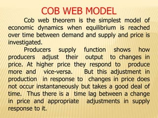
1. COB WEB MODEL
Cob web theorem is the simplest model of
economic dynamics when equilibrium is reached
over time between demand and supply and price is
investigated.
Producers supply function shows how
producers adjust their output to changes in
price. At higher price they respond to produce
more and vice-versa. But this adjustment in
production in response to changes in price does
not occur instantaneously but takes a good deal of
time. Thus there is a time lag between a change
in price and appropriate adjustments in supply
response to it.
2. The time gap between decisions to change in
the quantity supplied in response to a given price
and its actually being supplied is known as supply
lag. The supply lag is often found in case of
agricultural commodities .
The supply lag often result in Cyclical
movements or oscillations in price and quantity over
time. The dynamic analysis of stability investigates
whether these oscillations converge to equilibrium
values or move away from them.
3. Cob Web model: For instance, we consider for
sugarcane, where the supply of sugarcane is lagged
function of price. In order to keep our analysis
simple we assume that there is a one year lag in
the response of quantity supplied of sugarcane to
a given market price of it thus:
1. S=f(Pt-1)
The demand function there is no time lag that is
the quantity demanded of this year depends on
price of this year thus:
2. D=f(Pt)
4. It is used to explain the dynamics of demand,
supply and price over long period of time. The cob-
web model (or Theorem) analyses the movements
of prices and outputs when supply is wholly
determined by prices in the previous period.
As prices moves up and down in cycles, quantities
produced and also seem to move up and down in a
counter-cyclical manner (e.g. prices of perishable
commodities like vegetables).
In order to find out the conditions for converging,
diverging or constant cycles: one has to look at the
slope of the demand curve and then of the supply
curve.
5. Assumption
The cob-web Model is based on the following assumption:
1. The current year’s (t) supply depends on the last year’s (t-1)
decisions regarding output level.
2. Hence current output is influenced by last year’s price. i.e. P (t-1)
3. The current period or year is divided into sub-periods of a week or
fortnight.
4. The parameters determining the supply function have constant
values over a series of periods.
5. Current demand (Dt) for the commodity is a function of current price
(Pt).
6. The price expected to rule I the current period is the actual price in
the last year.
7. The commodity under consideration is perishable and can be stored
only for one year.
8. Both supply and demand function are linear .i.e. both are straight
line curves which increases or decreases at a constant proportion
6. The Cob-web Model : There are two types of Cob-web
Models:
1. Convergent
2. Divergent
3. Continuous
(1) Convergent Cob-web
Under this model the supply is a function of previous year
i.e. S= f (t-1) (‘t’ is the current period and‘t-1’ is a previous
period) and on the other hand the demand is the function of
price i.e. Dt=f (P). The equality between the quantity
supplied and quantity demand is called as Market
equilibrium. i.e. St=Dt. Equilibrium can be established only
through a series of adjustment if current supply is in
response to the price during the last year. But this
adjustment will take place over a several consecutive
periods.
7. For e.g. suppose we take the example of sugarcane growers
who is producing one crop in a year. The sugarcane growers
will grow this year on the assumption that the price of
sugarcane this year will be equal to price in the last year.
The market demand and supply curves for onions are
represented by DD and SS curves respectively in diagram.
8. Suppose the price in the last year was OP1 and Producers
decide the equilibrium output OQ1 this year. Now suppose
there is crop failure due to natural calamities which decrease
the output OQ2 which is less than OQ1 (i.e. equilibrium
output). Lack of supply will increase the price to OP2 in the
current period. In the next period, the onion growers will
produce OQ3 quantity in response to the higher price OP2.But
this is more than the equilibrium quantity OQ1 which is the
actual need of the market.
The excess supply will lower the price to OP3. This will
encourage the producer to change the producer plan, where
they will reduce the supply to OQ4 in the third period. But
this quantity is less than the equilibrium quantity OQ1. This
will lead to again rise in price to OP4, which in turn will
encourage the producers to produceOQ1 quantity.
9. The equilibrium will be established at point g where DD and
SS curves intersect. This series of adjustments from point
a,b,c,d,and e to f is traced out as a cobweb pattern which
converge towards the point of market equilibrium g. This is
also called as the dynamic equilibrium with lagged
adjustment..
10. (2) Divergent Cob-Web
The divergent cob-web is unstable cobweb when price and
quantity changes move away from the equilibrium posting.
This can be explained with the help of following diagram,
11. We will start with the initial equilibrium price is OP1 and
equilibrium quantity OQ1. Now suppose there is a temporary
disturbance that causes output to fall to OQ2. Due to lack of
supply the price will rise to OP2.
The increase in price will in turn raise the output to
OQ3 which is more than the equilibrium output OQ1. The
increase in supply will lead to fall in price to OP3. This fall in
price will increase the demand and there will be excess
demandOQ2 than supply. The excess demand will shoot up
the price to OP4. This shows that the price will be still away
from the equilibrium after the adjustment by the producers.
This is called as Divergent cob-web.
12. 3) Continuous cob-web
The cob-web models in this show the continuous changes in
price and quantities.
13. Suppose we start with the price OP1 as shown in the
diagram. As the supply will be more due to high price in
the market. On the other hand the demand will be less as
compared to the supply OQ2 and the demand will
reduced to OQ2.
The fall in demand will force the producer to decrease
price to OP2 in next period. But at this price OP2 the
demand will be OQ2 which is more than the supply OQ1
which reduced. This way the prices and quantities will
circulate constantly around the equilibrium.
14. POLICY IMPLICATIONS:
The stability of equilibrium of a market has important
implications for economic policy. If a competitive market
is in stable equilibrium it implies that it can survive any
external disturbances however large and drastic it may
be . That is if any disturbance causes disequilibrium in
the stable nature of market equilibrium ensures that
certain forces will automatically come into play to bring it
back into equilibrium.
This is a very important conclusion because if
market equilibrium is stable and automatic corrections of
disequilibrium is possible, theoretically there is no need
for government interfere in a free market equilibrium.
15. POLICY IMPLICATIONS:
In case unstable market disequilibrium free competitive
market could collapse under the pleasure of either high
inflation or recession. In fact in the real world we
witness un stable equilibrium in some commodity
markets. Foreign exchange market and therefore, rely
on self-correction by the market would not take place.
Therefore, the government interference is necessary to
achieve equilibrium with the stability in prices and higher
levels of income and employment.