SlideShare a Scribd company logo
1 of 47
Download to read offline
Empirically Calculating an
Optimal Hedging Method
Stephen Arthur Bradley
Level 6 project
20cp
Deadline: Tuesday 3rd May 2016
1
Acknowledgment of Sources
For all ideas taken from other sources (books, articles, internet), the source of the ideas is
mentioned in the main text and fully referenced at the end of the report.
All material which is quoted essentially word-for-word from other sources is given in quo-
tation marks and referenced.
Pictures and diagrams copied from the internet or other sources are labelled with a refer-
ence to the web page or book, article etc.
Signed . . . . . . . . . . . . . . . . . . . . . . . . . . . . . . . . . . .Date . . . . . . . . . . . . . . . . . . . . . . . . . . . . . . . . . . .
2
Contents
1 Introduction 4
1.1 Put Call Parity . . . . . . . . . . . . . . . . . . . . . . . . . . . . . . . . . 5
2 Volatility 5
2.1 Historical Volatility . . . . . . . . . . . . . . . . . . . . . . . . . . . . . . 5
2.2 Implied Volatility . . . . . . . . . . . . . . . . . . . . . . . . . . . . . . . 6
2.2.1 Volatility Smile . . . . . . . . . . . . . . . . . . . . . . . . . . . . 7
2.3 Comparison of Implied and Historical Volatility . . . . . . . . . . . . . . . 7
3 The Greeks 9
3.1 Delta . . . . . . . . . . . . . . . . . . . . . . . . . . . . . . . . . . . . . . 9
3.2 Delta Hedging . . . . . . . . . . . . . . . . . . . . . . . . . . . . . . . . . 9
3.3 Gamma . . . . . . . . . . . . . . . . . . . . . . . . . . . . . . . . . . . . 10
3.4 Vega . . . . . . . . . . . . . . . . . . . . . . . . . . . . . . . . . . . . . . 10
4 Black Scholes Model 11
4.1 Assumptions . . . . . . . . . . . . . . . . . . . . . . . . . . . . . . . . . 11
4.2 Black Scholes Equation . . . . . . . . . . . . . . . . . . . . . . . . . . . . 11
4.3 Option Pricing . . . . . . . . . . . . . . . . . . . . . . . . . . . . . . . . . 12
4.4 Delta Calculation . . . . . . . . . . . . . . . . . . . . . . . . . . . . . . . 12
4.5 Delta Hedging with Historical Volatility . . . . . . . . . . . . . . . . . . . 12
4.5.1 Hedging All Options . . . . . . . . . . . . . . . . . . . . . . . . . 14
4.6 Delta Hedging with Implied Volatility . . . . . . . . . . . . . . . . . . . . 17
4.7 Comparison of the Performance of Implied and Historical models . . . . . 17
5 Heston Model 20
5.1 The Feller Condition . . . . . . . . . . . . . . . . . . . . . . . . . . . . . 21
5.2 Euler-Maruyama Method . . . . . . . . . . . . . . . . . . . . . . . . . . . 21
5.3 Fast Fourier Transform . . . . . . . . . . . . . . . . . . . . . . . . . . . . 22
5.4 Model Calibration . . . . . . . . . . . . . . . . . . . . . . . . . . . . . . . 24
5.5 Hedging with the Fast Fourier Transform . . . . . . . . . . . . . . . . . . 26
5.6 Hedging with Euler-Maruyama Simulation . . . . . . . . . . . . . . . . . . 26
6 GARCH model 26
6.1 Model Features . . . . . . . . . . . . . . . . . . . . . . . . . . . . . . . . 27
6.2 Information Criterion . . . . . . . . . . . . . . . . . . . . . . . . . . . . . 30
6.3 Model Calibration . . . . . . . . . . . . . . . . . . . . . . . . . . . . . . . 31
6.4 Hedging with GARCH . . . . . . . . . . . . . . . . . . . . . . . . . . . . 33
7 Performance Comparison 36
7.1 Parameter Fitting . . . . . . . . . . . . . . . . . . . . . . . . . . . . . . . 37
7.2 Performance Statistics . . . . . . . . . . . . . . . . . . . . . . . . . . . . 38
A Black Scholes Delta Hedging Code 41
B Heston Delta Hedging Code 42
C GARCH Delta Hedging Code 45
3
Abstract
Hedging a portfolio describes any method which minimizes the risk of losses and
there are many methods of doing so. The methods we shall examine will focus on delta
hedging. This will require certain assumptions, for example, to define the behaviour
and the evolution of the unobserved volatility process. Further, we will have to assume
a model for the data and it is not clear which model will perform the ’best’ in practice.
Exploring the application of some different models we calculate that the simple his-
torical volatility model is one of the most impressive models for reducing risk but the
GARCH model clearly out performs others we have considered, especially when time
constraints are a limiting factor which they are in most real world applications.
1 Introduction
When a financial option is bought or sold there is always risk affecting the potential profit or
loss. The value of the underlying stock will change through time and the risk (with respect
to a purchased option) is that this will cause the value of the option to fall or even become
worthless. The risk with respect to a written (sold) option, is that an extreme movement in
the underlying stock price could leave the buyer with an unbounded profit and the writer
with the corresponding, unbounded loss. Hedging refers to any method which attempts to
eliminate/minimise the risk associated with a portfolio.
Calculating the hedge of an option can be a very complicated procedure. Thus, cer-
tain assumptions can be made to simplify calculations. One such assumption is that the
volatility of the underlying stock can be modelled by a constant function; this assumption
is made under the Black Scholes model. However, this particular assumption is very strong
and often assumed to be an over simplification of reality which result in inadequate and
unreliable forecasts and conclusions.
Further, a constant volatility of the stock implies a constant variance in the price pro-
cess. However, the trading price of the stock reflects the traders’ belief of the value of the
stock and this can be effected by many things. These beliefs are often very similar among
traders because they are all viewing the same available news about the company/stock.
Thus, we tend to experience some periods of extreme deviation in price and some periods
of gradual change; this would seem to be a contradiction and supports the notion of a time
varying volatility.
In general, a model in which the volatility is modelled by a time-dependent function
will be more flexible in an attempt to better explain the data. Thus, it seems reasonable
to assume that models with a non-constant volatility will outperform their counterparts in
forecasting accuracy and will be more relevant and justified. Through this project we shall
determine the benefit (if any) from using the more complicated model.
The aim of this project is to decide which model assumptions perform the ’best’ in a
practical sense. We will consider the hedging method and model assumptions as optimal if
they generate the greatest profit with the minimum risk. All calculations and methods will
assume the existence of a fair market in which there is no arbitrage (guaranteed profit).
In the following sections we shall first explain different methods for modelling and
estimating the volatility; historical (assuming constant), implied or stochastic. Then we
shall discuss some hedging techniques and elaborate on delta hedging specifically. We
will then explore the assumptions, features and equations of the models which we are
implementing, and finally, calculate and compare the resulting profits under these different
models and assumptions. Comparing the mean of the profits will show how successful
the portfolio is under each method and comparing the variance of the profits will give an
indication of the residual risk. We shall reach a conclusion of optimality by considering
both of these statistics. More specifically, the profit mean divided by its standard deviation
4
will be a strong indication of the performance of the model because a large value would
indicate a positive profit and a relatively insignificant risk. For large portfolios however, it
will also be important to consider the running time of the hedging algorithm.
1.1 Put Call Parity
Put call parity is a useful relation between the price of a call option and the price of its
corresponding put option; if we know either price, the formula allows us to calculate the
other.
Ct + K = Pt + St ∀t
A simple proof is as follows. If we possess the call option and an amount of cash equal
to the strike price, then at time T this combination will be worth:
(ST − K)+
+ K = max(ST , K)
Whereas, if we possess the corresponding put option and a share of the stock, our combi-
nation is worth:
(K − ST )+
+ ST = max(ST , K)
Since both combinations are equal in value at time T, they must also be equal at all
times before T, to avoid an arbitrage opportunity [6]. This can be proved by contradiction
as follows.
Assume that portfolio A and portfolio B have an identical value at time T, i.e. AT =
BT , and there exists a time t < T where A has a greater value than B (without loss of
generality), i.e. At > Bt. Then we could buy portfolio B and take a short position on A
(sell), then, at time T we can sell B to buy A and fulfil our short position. The overall profit
is given by:
−Bt + At + BT − AT = At − Bt > 0
This is guaranteed profit, so it contradicts the assumption of a fair market.
Hence, we must have that A and B are always equal in value.
2 Volatility
Volatility is a measure of how much a stock’s price is expected to deviate over a short period
of time. In general, many parameters in a financial model are known or readily available,
for example: the time until expiration, the strike price and the current stock price. Volatility
is the only unknown variable which contributes to the price of an option.
Consider an at-the-money option, an option with strike price equal to the current stock
price, then the price of the option will be an increasing function of the volatility. Thus, if
the volatility is an underestimate, the option will be under-priced and if we purchase this
option then the expected profit will be strictly positive. Similarly, if the volatility is an
overestimate and the option is overpriced then shorting the option will generate a strictly
positive expected profit. In either case, there is effectively an arbitrage opportunity. From
this, it is easy to see that effective volatility estimation is crucial to the profit or loss of a
portfolio.
2.1 Historical Volatility
Historical volatility is an estimate which models the volatility as a constant process and is
estimated solely from historical data of the evolving stock price. Historical volatility can
also be called realized or statistical volatility. One method of estimating this value is under
the assumption that the stock’s volatility is the standard deviation of the log returns of the
5
stock, where the return at time t is given by: St/St−1. Let Rt denote the returns, then we
have:
Rt := log
St
St−1
The sample variance of these log returns is then given by:
ˆσ2
=
1
n − 1
n
t=1
(Rt − ¯R)2
where the divisor is (n − 1) to give an unbiased estimate and ¯R is given by
¯R :=
1
n − 1
n
t=1
Rt
=
1
n − 1
n
t=1
log
St
St−1
=
1
n − 1
n
t=1
[log(St) − log(St−1)]
=
log(Sn) − log(S0)
n − 1
Thus, we have the standard deviation as;
ˆσ =
1
n − 1
n
t=1
(Rt − ¯R)2
The final step here is to annualize this volatility. This ˆσ gives the 1-day standard de-
viation so we shall annualize this value in order to use it in the formulae and also for
comparison with other estimates of the volatility. Under the assumption that the variance
will be the same each day, the annual variance will be the daily variance multiplied by 252;
this is standard convention since there are 252 trading days in a year. Equivalently, the an-
nualized standard deviation (annualized volatility) is equal to the 1-day standard deviation,
ˆσ, multiplied by
√
252. This gives the estimate of the historical volatility as:
ˆσannualized =
252
n − 1
n
t=1
(Rt − ¯R)2
Note that even on the weekends and holidays there are changes in the market due to
news or events and this will cause larger differences between Friday and Monday values
than one would expect from a typical one day jump. Thus, it would also be reasonable to
use 365 here as opposed to 252.
2.2 Implied Volatility
Implied volatility is estimated from the market price of the option using the Black Scholes
equation (discussed in section 4). The Black Scholes equation gives the fair price of an
option as a function of many parameters, including the volatility. Thus, if we know the
current price of the option then the only value which is unknown is the volatility. We can
then set our estimate of the volatility, ˆσt, as the value of σ for which the Black Scholes
equation gives the observed price. This is where Implied volatility gets it’s name, i.e. it is
the value of the volatility as implied by the option price under the Black Scholes equation.
6
2.2.1 Volatility Smile
What is interesting about the implied volatility is how it changes with the strike price, i.e.
how the implied volatility changes depending on how in-the-money or out-of-the-money
the option is. An option is called in-the-money if exercising it at the current time would
generate a profit and out-of-the-money if exercising the option would generate a loss. This
relationship is shown in Figure 1.
Exercise Price
18 20 22 24 26 28 30 32 34 36 38
ImpliedVolatility
0
0.1
0.2
0.3
0.4
0.5
0.6
0.7
0.8
0.9
1
Volatility Smile for selected call options
Figure 1: Volatility smile for a section of the data; i.e. the strike price against the implied
volatility for all options which become available on the 24th of April 2014 and which expire
on the 30th of May 2014. Where the vertical line represents the current stock price (the
price of the stock on 24th of April)
This Figure shows that there is a clear relationship; the volatility seems to be an almost
symmetrical, gradually increasing function of the difference between the strike price and
the current stock price.
There is a subtle problem with this pattern because the current price is not in the centre
of the curve. However, the ”current” stock price process we have access to was recorded at
the end of each trading day, and the closing hours of a trading day are the most busy. This
means that, the changing price process on each day of busy trading, has been approximated
by a single value. Thus, although the process will be roughly representative of the true
price process, we can expect small deviations from the most reasonable answers. In short,
the current price line in Figure 1 indicates the last recorded value of the stock at the end of
the day, but perhaps a more representative value for that day would have been in the centre
of the curve.
2.3 Comparison of Implied and Historical Volatility
The No-Arbitrage principle assures us that the volatility of an option will give the fair
price, i.e. the price for which the expected overall profit will be zero. In reality however,
the seller/writer of the option will be intending to make a profit, thus, the price will be
a little higher than the fair market price. This means that the implied volatility and the
realized (historical) volatility will take different values by design.
Note that the price of an option is always an increasing function of the volatility as
illustrated by Figure 2. Since the volatility is the only unobserved quantity, this figure
7
shows that increasing the price of the option is identical to increasing the assumed value of
volatility.
Hence, by increasing the price of an option above the fair market price, the writer of
the option has increased their implied volatility. This suggests that implied volatility will
always exceed the true volatility of the market. Since the historical volatility is an unbiased
estimate of the true volatility, we would expect the seller of the option to make a profit if
the implied volatility exceeds the historical volatility.
This implies that the seller is expected to loose money when their implied volatility is
lower than the current historical volatility. Equivalently, this situation yields an expected
profit for the buyer and this will effectively be arbitrage if the variance is sufficiently small.
As we are hedging these options, we are assuming the role of the seller (taking a short
position) so it is important to check this feature. The comparison is shown in Figure 21.
120
110
Stock Price
100
surface plot illustrating that the
option price increases with volatility
90
800
0.2
Volatility
0.4
0.6
0.8
60
100
40
20
0
80
1
OptionPrice
Figure 2: Black Scholes price for a call option with changing volatility and strike price
Time (days)
20 40 60 80 100
volatility
0
0.5
1
1.5
2
2.5
3
3.5
4
Comparison of historical and implied volatility
Implied
Historical
Time (days)
20 40 60 80 100
volatility
0
0.1
0.2
0.3
0.4
0.5
Comparison of historical and implied volatility
Implied
Historical
Figure 3: Historical and Implied volatility for the dataset
8
From Figure 3 we can see that very few options have an implied volatility below the
estimates of realised volatility. From the above, this implies that the vast majority of these
options will expect a positive return. This is an expected result and motivates the writing
of options.
3 The Greeks
Once we decide on a model for the volatility process and for the evolution of the stock price,
we can then hedge the portfolio. However, there are various methods to choose from before
in order to hedge an option. Each method depends on certain financial objects, known as
Greeks. These objects are referred to as Greeks simply because most financial objects of
this type are denoted by Greek letters, [8]. In this section we shall consider some of them
and elaborate on some hedging methods.
3.1 Delta
An option’s delta is the change in the price of the option for every unit change in the price
of the underlying stock, i.e. an indication of the sensitivity of the option to the stock price.
For example, if an option has a delta of 1
2 and the price of the underlying stock increases
by x, the price of the option will increase by 1
2 x.
Consider the effect of an increasing stock price on call and put options. The pay off
of a call option is given by (ST − K)+
so every increase in St increases the expected pay
off of the option. Under the assumptions of a fair market, the price of the option will then
increase which indicates that call options have a positive delta.
On the other hand, a put option has a pay off of (K − ST )+
whose expected value will
decrease as the stock price increases. Under the same assumptions, the price of the option
will decrease. Thus, put options have a negative delta.
Furthermore, consider an in-the-money call option. Then, as time, t, approaches T
(the expiration date) there will be a pay off of (ST − K)+
≈ St − K and clearly this is
linear in St so an increase of 1 in the stock price would increase the pay off by 1, and so,
increase the option price by 1. This implies that the delta of a call option tends to 1 as t
tends to T.
Similarly, consider an in-the-money put option. The pay off of this option is (K−St)+
and will tend to K −St as t tends to T, thus, each unit increase in the stock price will result
in a unit decrease in the option price. This shows that the delta of an in-the-money put
option tends to -1 as t tends to T.
3.2 Delta Hedging
As above, an option’s delta is equal to the change in value of the option per unit change
in the underlying stock price. Thus, if we write (sell) an option and calculate it’s delta at
present time to be δ, then we can hedge the option by shorting (selling) δ shares of the
stock.
After doing this, a unit increase in the stock will increase the option’s price by δ and
will cause us to loose δ by shorting the stock, thus, the value of the portfolio will change
by δ-δ=0. When this holds, we say that the portfolio is delta neutral. This shows that all
risk has theoretically been eliminated and confirms the validity of the hedging method.
However, the delta of an option is not constant, so the number of shares of the under-
lying asset will need to be continually updated. This is a little impractical and in reality
there will be transaction fees when buying/selling shares of the stock. For simplicity, in our
calculations, we shall not consider transaction fees but, so that the results and conclusions
are useful in a practical sense, we shall only implement the hedging method at the end of
each day, i.e. we shall update the number of shares held in the portfolio once per day.
9
3.3 Gamma
It is clear that the delta of an option will not be the only important quantity. In general,
the value of the option cannot be expected to change as a linear function of the stock price.
We can generalizing this method to also include the second derivative of the stock price
process.
An option’s gamma is a measure of the sensitivity of the delta to the stock price, the
change in the value of delta per unit change in the stock price, which defines gamma as a
second derivative risk [8]. If we consider delta as the speed the option price changes with
respect to the stock price, then we can consider the gamma as the acceleration of the option
price with respect to the stock price.
Since gamma is a second derivative of an unobserved quantity, estimation of the value
of gamma will be very difficult and more likely to be inaccurate - apart from in some simple
cases.
3.4 Vega
Similar to delta, an option’s vega, denoted ν, is the change in the option price per unit
change in volatility.
This method deals with a different type of risk. As we have seen in Figure 2, the
volatility can have a strong impact on the value of an option. This suggests that an increase
in the market volatility will increase the value of the option by increasing the expected
profit. More specifically, if we were to write an option when the volatility was low then we
would have to sell it at a low price but if the volatility increased then our potential losses
would also increase.
To hedge this type of risk and calculate a vega neutral position, we will need to buy a
certain number of options.
The number of options to buy will be a very difficult quantity to measure because it
will depend sensitively on the volatility process, which is unobserved and estimated in a
number of ways.
10
4 Black Scholes Model
4.1 Assumptions
The assumptions under the Black Scholes Model are as follows.
• Volatility of the stock, σ, is constant in time
(this is the most important and controversial assumption)
• No dividends are paid to the stock owner
• The interest rate is a known constant, r
• No transaction fees, so buying and selling stocks is free
• Liquidity is such that any amount of any stock can be bought or sold at any time
However, the model can be manipulated in order to be more useful in real life applications.
For example, the constant volatility can simply be replaced by the implied volatility or by
a stochastic volatility measure.
4.2 Black Scholes Equation
The Black Scholes partial differential equation states the following.
dS = S(µdt + σdW)
where St denotes the price of a stock at time t, µ denotes the drift, σ denotes the stock’s
volatility and Wt is a Brownian motion with distribution N(0, t). A solution to this equa-
tion must take the form:
St = Aeµt+σWt
where A is a constant.
Setting t=0 we can see that A must equal S0 (the initial value of the stock), i.e.
St = S0eµt+σWt
Let S∗
t denote the discounted pay off such that S∗
t = Ste−rt
.
Then we have:
E(S∗
t ) =e−rt
E(St)
=e−rt
E(S0eµt+σWt
)
=S0e(µ−r)t
E(eσWt
)
=S0e(µ−r)t
E(eN(0,σ2
t)
)
=S0e(µ−r)t
e
σ2t
2
=S0e(µ−r+ σ2
2 )t
Hence, when µ = (r − σ2
2 ), S∗
t will be a Martingale. This is a desired property to ensure
that the stock price can be expressed as follows.
St = S0e(r− σ2
2 )t+σWt
11
4.3 Option Pricing
Here, we consider only European Call options, in which the call can only be exercised on
the expiration date and not before. A European Put option can be calculated by first finding
the price of the corresponding call option and invoking Put-Call Parity.
Let K denote the strike price for the option, S0 denote the current stock price, T the
time until expiration, and let r denote the fixed interest rate.
Then the option price is calculated as follows.
d1 :=
log(S0
K ) + T(r + σ2
2 )
σ
√
T
d2 :=
log(S0
K ) + T(r − σ2
2 )
σ
√
T
The price of the call option is given by:
C(S0, T) = S0Φ(d1) − Ke−rT
Φ(d2)
and the price of the corresponding put option is:
P(S0, T) = Ke−rT
Φ(−d2) − SΦ(−d1)
4.4 Delta Calculation
In order to implement a delta hedging technique we will need the ability to calculate delta
for European options. Under the Black Scholes model, the delta of a call option is given
by: Φ(d1) where Φ(-) represents the cumulative distribution function of a standard Normal
random variable and d1 is as above, i.e.
δ = Φ
log(S0
K ) + T(r + σ2
2 )
σ
√
T
Similarly, for put options we have delta as Φ(d1).
This is obvious from the above expressions for C(S0, T) and P(S0, T) when we recall
that the delta is simply the differential of the option price with respect to the stock price,
S0.
Figure 4: Resulting profit from delta hedging the options using historical volatility and the
Black Scholes model
4.5 Delta Hedging with Historical Volatility
The first hedging method we shall implement is the Delta Hedging method under the Black
Scholes model, with the volatility estimated by the historical volatility. From this point on,
for simplicity, we shall assume that the interest rate, µ or r, is equal to zero.
12
For each individual option in the available portfolio, the value of delta is calculated
(under the Black Scholes assumptions) at the end of each day and the option is hedged
accordingly. For a call option this corresponds to buying delta shares of the stock and for
a put option this corresponds to selling (taken a short position) on delta shares of the stock
at the current (end of day) price. In either case, the value of delta needs to be calculated in
a different way.
This hedging technique has been applied to all options which expire in at least 5 days
and the options with a expiry of 4 or fewer days have not been hedged, this is again for
practical purposes because we are assuming that it is not a profitable use of time to hedge
an option which expires in only a few days. This is a reasonable and common approach.
Figure 5: The time (in days) until expiry of those options with an absolute profit which is
larger than 1.5
The histogram of resulting profit/loss, displayed in Figure 4, illustrates the consistency
of the results and confirms that this method eliminates the vast majority of the risk involved
in writing these options (as is the methods purpose). Most values are close to zero, as we
would expect, and most are positive which is encouraging.
This method is further supported by the histogram in Figure 5 which shows that almost
all (1357/1403) of the options resulting in an extreme profit/loss, expire within less than 5
days of purchase (where an absolute value greater than 1.5 is classified as extreme, since
1.5 is the average price of an option). This means that they have not been hedged; for a
practical approach as previously stated. Thus, the vast majority of the variance is due to
options which were not hedged and this is a significant result because the options which
were not hedged make up only 12.7% (3349/26388) of the total number of options.
Since almost all the variance is due to a lack of hedging, it may be more useful to ex-
plore the analysis of only the hedged options.
The hedged options have a mean of 0.0512 and a standard deviation of 0·083. The
value 0.0512 seems insignificant but it is close to zero by design (in minimising the risk we
decrease the potential profits). Also, it is greater than zero and since the standard deviation
is fairly small, this profit is consistent enough to effectively be called arbitrage.
This mean is not as insignificant as it appears. The average profit is equal to 3.44%
of the average option price which is an impressive degree of arbitrage. Thus, we must
conclude that this method functions very well, in fact, this has shown a very promising
result and suggests that we could enjoy significant improvement in our profits by relaxing
our rule for practicality, i.e. hedging options of any expiry date.
To decide if this would be best suited to our purposes, we shall now analyse the effects
of the exhaustive approach more closely.
13
Option (time ordered) #104
0 0.5 1 1.5 2 2.5
Profit
-3
-2
-1
0
1
2
3
Historical volatility approach
compared with no hedging method
Figure 6: Contrast of the profit of hedging all options when using Black-Scholes and his-
torical volatility (yellow) as opposed to not applying a hedge (blue)
4.5.1 Hedging All Options
From Figure 7 we can see that abandoning our practical approach has significantly reduced
the variance in the profits (from 0.4596 to 0.0080) but has also significantly reduced the
potential profit. It is interesting that the median does not seem to have significantly changed
(0.0154 from 0.0162) which suggests that there are roughly equal numbers of profits and
losses in each case. This is expected because hedging methods are designed to eliminate
risk and not to turn losses into profits or to maximize profits.
An important consideration of hedging is that someone who is going to the trouble of
hedging a portfolio, is likely to apply the method to a large number of options. This sug-
gests that, assuming the standard deviation of profits is sufficiently low, the only important
value is the mean profit. Here, we have that the mean profit has changed from 0.1229 to
0.0478. This is an extremely important result because, the average profit has been reduced
to a third of its original size.
Note that we are not suggesting the only important quantity is the mean.
If we were to sell these options with no hedging method, the resulting profit
would have mean 0.0601 but this does not imply that no hedging method at
all is better than our historical volatility approach. This is clear
from the graph in Figure 6 which clearly shows how the risk has been minimised.
In practice, this is always an unwanted side effect when hedging a portfolio and can be
seen as the cost of a safe, risk free portfolio. Figure 6 illustrates how hedging methods will
14
control the risk and simultaneously limit the profits. The initial losses shown in the hedged
options are likely to be largely caused by the temporarily high volatility in the underlying,
shown by the extreme profits and losses of the ’unhedged’ options in blue.
Since the short-term options generate a larger profit when they are not hedged, this idea
of the importance of the mean suggests that the application of a hedging method is not the
optimal decision when the option is only available for a small number of days. Also note
that we have not included transaction fees in our model which would give further evidence
to the practical approach. However, this approach, in a hedging framework, implies that the
profit from these short-term options is not exposed to risk. This is a very bold assumption
to make for any option since it contradicts the assumption of a free market; that there are
no arbitrage opportunities. Nonetheless, we are searching for the most practical approach
so we shall examine the evidence before discarding the method.
Practical Hedge All
Profit
-2
0
2
4
6
8
10
12
Hedging with Black-Scholes and Historical volatility
Figure 7: Box diagrams comparing the practical method to the method of hedging all
options, when using Black-Scholes and historical volatility
We could argue that these profits are unaffected by risk if they are consistently positive
and are independent of the market. Figure 8 shows a close up of the histogram of profits
(short-term options only) when we do not hedge. This suggests that there is still risk in-
volved because a reasonable number are ending in a loss. However, the histogram is a little
misleading because the bar between −0.02 and 0.04 consists of over 2200 options. Thus,
these options are very consistent but this level of consistency doesn’t imply risk free.
To decide whether the series depends on the market behaviour we would like to know
if the price process is correlated with the profits from the short-term options. We can cal-
culate the mean profit from these options, daily, and compute the cross correlation between
the price process, and this sequence of mean profits. This cross correlation is plotted in
15
Profit with no hedge
-1.5 -1 -0.5 0 0.5 1 1.5 2
Frequency
0
10
20
30
40
50
60
70
80
90
100
Histogram of unhedged, short-term options
Figure 8: Histogram showing the profit from short-term options (under 5 days) when un-
hedged.
Figure 9 using a rough indication of significance which relies on a null hypothesis that the
true correlations are zero with a variance of 1/sqrt112, since 112 is the length of this time
series. The Figure shows that the market behaviour (represented by the price process of the
stock) appears to be weakly correlated with these average profits.
Lag, in the Figure, is referring to the price process, e.g. at lag K, we are examining the
expectation:
E( [Xt−K − ¯X] · [Pt − ¯P] )
E( [Xt − ¯X]2) · E([Pt − ¯P]2 )
where X,P represent the price process and profit process respectively.
The most important feature of the cross correlation, is that there is a significant negative
correlation for negative lags. Although the correlation is only briefly significant, this is
extremely important because it shows that the past of the market behaviour is correlated
with the present profits. This implies that the profits from these options depend on market
behaviour and so, cannot be considered as risk free arbitrage opportunities. In a hedging
framework, minimizing risk is the most important goal, thus, the most sensible thing to do
here is to be cautious and assume that the correlation is significant.
To conclude this section, we shall surrender our practical approach of only hedging
certain options. Instead, we shall exchange potential profits for security, and hedge all
available options.
16
Lag
-100 -80 -60 -40 -20 0 20 40 60 80 100
Correlation
-0.25
-0.2
-0.15
-0.1
-0.05
0
0.05
0.1
0.15
0.2
Cross correlation between the price process
and the average daily profit from short-term options
Figure 9: Cross correlation of the observed price process with the series of daily mean
profits from short-term options.
4.6 Delta Hedging with Implied Volatility
This method has been calculated in the same way as the previous method but with an
implied volatility instead of the historical volatility. It seems reasonable to expect that this
method will perform better than the previous method purely due to the increased flexibility
of the implied volatility.
From our previous conclusion, we shall now consider hedging all options in the portfo-
lio; in order to make a fair comparison. Since we have shown that a simple histogram can
be misleading, we shall consider a comparison similar to that of Figure 6. This comparison
is shown in Figure 10.
4.7 Comparison of the Performance of Implied and Historical models
Figure 10 shows a very similar structure to that of Figure 6 but contains some subtle differ-
ences.
Firstly, the initial options generate a significant loss under historical volatility, due to
the previously mentioned reasons, but under implied volatility we do not incur such losses.
The difference here is entirely due to the independence structure of the volatility process.
We calculate each value of implied volatility from the market data at that time as opposed
to accumulating a large amount of data to sufficiently estimate its value under a historical
model.
Another difference is that many of the profits are greater than those under the historical
volatility model. This is not obvious from Figure 10 so we shall use a different visualiza-
tion. Collecting all options which are available for an identical number of days, we can
much more easily observe and compare the effects of historical and implied volatility un-
der the Black-Scholes model. This plot is shown in Figure 11. This plot shows that under
implied volatility, the generated profit is almost always greater.
17
Option (time ordered) #104
0 0.5 1 1.5 2 2.5
Profit
-3
-2
-1
0
1
2
3
Implied volatility approach
compared with no hedging method
Figure 10: Contrast of the profit of hedging all options when using Black-Scholes and
implied volatility (yellow) as opposed to not applying a hedge (blue).
To explore whether this method has out performed the historical volatility model we
shall examine the statistics.
model variance mean
Historical 0.0095 0.0478
Implied 0.0181 0.0666
Firstly, the mean is greater under the implied volatility model, as expected from Figure
11. More interestingly however, the variance of the generated profits has more than dou-
bled. We could argue, as before, that both variances are very low so the only meaningful
comparison is that of the mean but this would be a minimalist approach. Comparing these
outputs using box diagrams, in Figure 12, indicates the distribution of profits.
It is obvious that the increased variance is caused by an increase in the number of pos-
itive ’outliers’, i.e. values exceeding the 75th percentile of the data. This is clearly visible
from the diagram because the outliers (red crosses) in the positive y-axis, referring to posi-
tive profit, have become much more dense. This increased number of larger profits will be
responsible for the increased mean. However, there has also been an increase in the number
of negative outliers which is indicated by the density of the negative outliers. This feature
of rough symmetry implies that the profits gained have been at the expense of risk.
In our calculations, the implied volatility of each option has been independent of all
previous data. This feature is largely responsible for the models success but could also be
considered as a problem in some cases.
18
Number of days from availability until expiry
0 5 10 15 20 25 30 35 40 45 50
Profits
0
10
20
30
40
50
60
70
80
90
Profit per length of availability
under Historical and Implied volatility
Figure 11: Comparison of the profits under implied and historical volatility using bins of
identical lengths (in days) of availability
When fitting a model, sometimes we observe a strange, unexpected change in the pa-
rameters, e.g. in the fitted value of volatility, which seems like an anomaly when compared
to previous patterns. Under a historical volatility model, we assume that the volatility is
constant, which implies that all data are equally important and so, estimates which seem
extreme will borrow strength from all previous data, i.e. more extreme values would be
stabilized via a running mean with all previous values. When we have a sufficient amount
of data, this would effectively bury the anomaly without the need for extra effort. The prob-
lem is that these extreme values cannot be corrected or buried under the implied volatility
model.
The flexibility of a model to allow for a time-dependent volatility is very attractive and
has proved very powerful. Thus, we shall maintain the assumption that the volatility is
time-dependent.
However, in order to include this idea in a model, we shall consider a consistent proba-
bility structure for the volatility. This can be done under the Heston model.
19
Historical Implied
Profit
-0.6
-0.4
-0.2
0
0.2
0.4
0.6
0.8
1
1.2
Profits under historical and implied volatility models
Figure 12: Box diagrams comparing the resulting profits when using the Black-Scholes
model with historical volatility and with implied volatility.
5 Heston Model
This model takes a different approach to volatility. Previously, we have allowed volatility to
be non-constant via considering the implied volatility to allow more flexibility in the model.
Volatilities calculated in this way will not depend on one-another, and so, the volatility
process could change sharply at every step. Although volatility represents randomness in
the price process, the volatility process itself should admit some form of structure and a
totally random, independent structure does not seem very justifiable. Here we shall allow
for a volatility structure which evolves slowly through time.
This model is not as widely implemented as Black-Scholes because it is more complex;
this is due to the added complication of the stochastic volatility as opposed to the very
simple idea of a constant one. The model is defined by the differential equations shown
below.
dSt = µStdt + σtStdW
(1)
t (1)
dvt = −γ(vt − θ)dt + κ
√
vtdW
(2)
t (2)
dW
(2)
t = pdW
(1)
t + 1 − p2dW
(3)
t (3)
Where the parameters are defined as follows;
S represents the stock price process
µ is the drift parameter, representing the interest rate
20
σ is the time dependent volatility
v is the variance, i.e. vt = σ2
t for convenience,
since a solution to equation (1) depends only on σ2
t , and not σt
θ is the long run mean of v
γ is the rate of relaxation to this mean
κ is the ’variance noise’
W(1)
and W(2)
are correlated 1-dimensional Brownian Motions
p is the degree of correlation between W(1)
and W(2)
, as enforced by equation (3) in
which W(3)
is another standard Brownian Motion independent of W(1)
and W(2)
[1].
5.1 The Feller Condition
Here is a short and simple result worth mentioning. The Feller condition states that:
2γθ > κ ⇒ the process vt is strictly positive
From the formula alone it is clear that this is a necessary result because the square root
of vt (i.e. σt) is used and appears in Formula (1). Also, from the concept of volatility
(behaving similarly to a standard deviation) we understand that negative values would not
be intuitively meaningful. This is an extremely important feature of the model and can
act as a quick check for the validity of fitted/assumed parameters. Alternatively, this con-
dition could be written as a constraint in a constrained optimisation problem, as we shall
implement in our model calibration.
5.2 Euler-Maruyama Method
The Heston model is not as commonly used as Black Scholes due to it’s increased com-
plexity and the computational cost of it’s application, for example, there is no closed form
expression for the price of an option under the Heston model. Thus, we will need a way to
simulate the the evolution of the price process and estimate the price of the option.
As mentioned above, we shall simplify this model by setting the interest rate, µ, equal
to zero. This gives:
dSt =
√
vtStdW
(1)
t (4)
dvt = −γ(vt − θ)dt + κ
√
vtdW
(2)
t (5)
Thus, assuming these parameters are known, a simultaneous realisation of {St}t>0 and
{vt}t>0 can be simulated using the Euler-Maruyama Method [7].
The Euler-Maruyama Method is used to simulate stochastic processes from stochastic
differential equations (SDE’s). The application of this algorithm is explained below.
1. replace dSt and dvt with S (t + 1) − S (t) and v (t + 1) − v (t), respectively
2. replace dt with 1
252 to annualize (there are 252 business days per year)
3. make S (t + 1) and v (t + 1) the subjects of the equations
4. generate the process iteratively from equations 4 and 5
This results in equations:
S (t + 1) = S (t) + v (t)S (t)
(1)
t
v (t + 1) = v (t) − γ [v (t) − θ]
1
252
+ κ v (t) p
(1)
t + 1 − p2 (2)
t
21
where S(0) refers to the current stock price, v(0) refers to the current volatility and
(1)
t ,
(2)
t are independent, Gaussian noise processes with mean zero and variance 1
252 ; since
the length of the interval is 1
252 in years (considering only trading days).
Note that S(0) is known and v(0) can be estimated by the current market volatility
(current estimate of historical volatility).
Assuming that the parameters are known (or estimated/fitted), we can use the Euler-
Maruyama method above to simulate the future of the process.
Further, the hypothetical profit can be calculated for each simulation and an average
should be roughly equal to the expectation of the resulting profit; by the weak law of large
numbers under the assumption that the parameters are adequately estimated. That is to say,
we can use this algorithm to give good estimates of
E(ST − K)+
and E(K − ST )+
for call and put options respectively.
By the assumption of a fair market, this expectation will be equal to the fair price of the
option at the present time. Then we could calculate a delta hedge for the options from the
following formula:
∆(St) = lim →0
C(St + ) − C(St)
(6)
and we can approximate this by taking a very small .
Clearly this will be very sensitive to errors in the price of the option so we will have
to decide on a reasonable number of iterations in order to balance this crucial issue of
accuracy with computational efficiency. This issue is especially important because we are
considering a large portfolio of over 26,000 options which means that the algorithm will
have to run over 26,000 times.
Ultimately, however, the focus will be on accuracy and the algorithm will be required
to perform an extremely large number of calculations. Such a problem makes this method
rather impractical.
5.3 Fast Fourier Transform
The Fast Fourier Transform (FFT) is a powerful solution to this problem of efficiency.
The FFT significantly reduces this computational cost and makes the model much more
attractive and is likely to be the main cause for the popularity of the Heston model.
Take f(·) as the density function of the log-return of the underlying price process, then
(subject to the assumption that f is an integrable function) the Fourier transform of f is
given by:
F(φ) =
+∞
−∞
eiφx
f(x)dx
f(x) =
1
2π
+∞
−∞
e−iφz
F(φ)dφ
where F is the characteristic function of f, [3].
The FFT method is very practical in calculating summations of of the form:
n
h=1
ei 2π
n (h−1)(k−1)
g(h) (7)
for some function g(·), [3].
This is useful to us because the fair price of a call option is given by:
22
C(St) =E (ST − K)+
=
+∞
−∞
(ST − K)+
f(log[ST ])d(log[ST ])
=
+∞
log(K)
(ST − K)f(log[ST ])d(log[ST ])
=
+∞
log(K)
(elog[ST ]
− elog[K]
)f(log[ST ])d(log[ST ])
=
+∞
log(K)
(exT
− elog[K]
)f(xT )dxT
which can be efficiently approximated by a sum in the same form as (7).
After some extensive calculus, Moodley [3] gives us the following form of the charac-
teristic function, under the Heston model.
CT (ku) ≈
e−αku
π
N
j=1
e− 2π
N (j−1)(u−1)
eibvj
FCT
(vj)
η
3
(3 + (−1)j
− δj−1)
The value of delta will need to be estimated here and will be very sensitive to changes/errors
in the price of the option; this approximation of the call price will clearly need to be very
accurate.
Although this method suggests that estimates will be calculated extremely quickly, we
must question whether this method is appropriate here. FFT methods are very useful in sig-
nal processing because they will determine which frequencies are present in the time series
and the amplitude of each frequency, [2]. This has many applications but in order to apply
it here, we must assume that the daily stock prices can be decomposed into sinusoids of
different frequencies. It is not clear if this assumption makes sense due to the unpredictable
nature of the stock market. An attempt at a justification may be that the stock price is so
unpredictable that we can treat it as a highly noisy process composed of many different
frequencies of noise but this is not an intuitively sound justification.
23
5.4 Model Calibration
In order to calculate a hedge as before, we must calculate the value of delta. To perform
this calculation, we require the parameters of the Heston model. Thus, the parameters of
the Heston model will need to be estimated from the data, i.e. calibrated to the data. For
each day, we can use a simple method to fit the parameters on that day. Under our current
assumptions, the parameters (i.e. γ, θ, κ, p) are constant in time so it seems contradictory to
make separate estimates each day but this will help us to see if their structure is consistent
and to test our assumptions.
All parameters for a given day are calibrated to the options which become available on
that day.
A simple calibration method is to take the set of parameters (along with a value for
the instantaneous volatility) for which the estimated option value is closest to the observed
option prices. That is to say, on a day where n options become available, we will take the
parameters, φ, that minimise:
n
i=1
[Observed option price − FFT(φ)]2
where FFT is a function to estimate the value under the Heston model. These fitted param-
eters are shown in Figure 13.
Days (2nd Jan - 5th June, 2014)
0 10 20 30 40 50 60 70 80 90 100
Parametervalue
0
0.5
1
1.5
2
2.5
3
3.5
4
4.5
5
Fitted Heston Parameters
instantaneous volatility
rate of relaxation (gamma)
long run mean (theta)
volatility of volatility (kappa)
correlation (p)
Figure 13: Calculated daily parameter values for the Heston model
On the whole, the Figure seems to clarify that this fitting technique is sufficient because
each curve has such a consistent structure. The only problem with this consistency is the
sharp spikes, which appear in all model parameters (γ, θ, κ and p) in a synchronized way
at about three different days; this is not a disaster because there is a total of 107 days in
which options become available.
These unexpected jumps in all model parameters do not appear in the estimate of the
instantaneous volatility. This suggests that the spikes could not have been caused by some
24
news or event involving the underlying stock. To elaborate further, these discontinuities
occur on the following dates: 28-Jan, 19-May and 05-Jun. Usually we would associate
such jumps in volatility structure with the anticipation of an event. For example, in the lead
up to an earnings announcement we can expect the (implied) volatility to rise because the
writers of the options want to limit the potential risk in case the earnings announcement
has a significant impact on the market. However, these announcements for the first and
second quarter occurred on April 17th and July 18th. So we can expect some other news,
maybe news which is indirectly related to this stock, to be the cause of this if it is not
simply an error in our calibration. For this reason, we shall consider sharp changes as an
error in model fitting; it is not unreasonable to expect some anomalous results here since
our method was so minimal.
Formally, we shall use the following condition. If the estimate of a parameter, on day
m, has increases by 100% of its original value, on day m − 1, then we shall say that the
estimate for day m is an anomaly and we shall replace its value with the original estimate
from day m − 1. Removing each anomaly in this way results in the estimates to the left of
Figure 14 which are arguably more reliable.
Days
0 20 40 60 80 100 120
0.1
0.2
0.3
0.4
0.5
0.6
0.7
0.8
0.9
Parameters with each anomaly removed
Days
0 20 40 60 80 100 120
0.1
0.2
0.3
0.4
0.5
0.6
0.7
0.8
0.9
Smoothed Parameters
gamma
theta
kappa
p
Figure 14: The graph to the left shows the daily estimates of the Heston parameters with
each anomaly removed, and the graph to the right shows the smoothed parameters, i.e. a
running mean of the estimates.
Defining an anomaly in this way does not seem to have completely solved the problem
for parameter theta since we still see some spikes, especially towards the end. However, the
estimated value of theta does appear to gradually increase towards the end so it seems that
the difference is systematic rather than an anomaly. An evolving structure would contradict
our model assumptions but this gradual change does not seem significant enough to stop
our model from being effective.
Considering that the structure of each parameter is assumed to be constant, we can
go a step further and smooth the daily estimates for the parameters using their running
mean (mean of all previous estimates). This method results in the estimates on the right
of Figure 14. These look convincing and we will use both sets of parameters to compare
hedge performance.
25
5.5 Hedging with the Fast Fourier Transform
For each set of parameters we can use the FFT to quickly estimate the price of the call
option and we can use put call parity to calculate an estimate of the value of a put option.
This seems to give a few strange mistakes when the option is only available for a small
number of days, e.g. sometimes estimates a negative value for the option. This could be
corrected by hedging the options until there is only a small number of days remaining,
although, we have illustrated the importance of hedging every option at all times in section
4.5.1, so we shall not leave any options unhedged.
5.6 Hedging with Euler-Maruyama Simulation
Although fairly impractical, the Euler-Maruyama method allows us to perform a simple
procedure which will not experience strange errors; given a sufficient number of simul-
taneously simulated chains with a sufficiently small value of in our approximation to
formula 6.
At each point, I have chosen to run 1,000 parallel simulations with 100 iterations in
order to estimate each option price. Then Formula 6 (Euler Maruyama equations) can be
used with a small value for epsilon, I have chosen 0.0001, to estimate the value of delta.
This algorithm has taken multiple hours to compute and has not proved very practical.
6 GARCH model
The Generalized Auto-Regressive Conditional Heteroskedasticity (ARCH) model with pa-
rameter q is defined by the equations below.
yt = log(St/St−1) = σt t σ2
t = ω +
q
i=1
αiσ2
t−i +
p
j=1
βiy2
t−j
where St denotes the stock process, σt denotes the volatility process and t is a white noise
process with mean zero and variance one.
The GARCH model is termed: a conditional variance model, this comes from the
feature below.
σ2
t+1 = ω +
q
i=1
αiσ2
t+1−i +
p
j=1
βiy2
t+1−j (8)
Notice that no estimation needs to take place here because all errors in this sum have
been observed, so this will be the true value and not an estimate. In other words, condi-
tional on the past and present data, the subsequent value of the volatility is known.
The features discussed below are present in the returns, St − St−1, and the relative
returns, St−St−1
St−1
, but we will apply the model to the log returns because this will allow a
useful additivity feature:
K
t=1
yt =
K
t=1
log(St/St−1) =
K
t=1
log(St) − log(St−1) = log(SK) − log(S0)
This alteration is for convenience but does not cause any problems in the model fitting
because the log returns are roughly equal to the relative returns [5]. This is shown below
via the Taylor expansion of the log function.
26
log(St/St−1) = log 1 +
St − St−1
St−1
=
St − St−1
St−1
−
St − St−1
St−1
2
+
St − St−1
St−1
3
− ...
≈
St − St−1
St−1
This approximation holds in practice because the returns tend to be very small in com-
parison to the stock price.
6.1 Model Features
One feature which most models don’t explain well is how the volatility process in a finan-
cial market tends to form clusters of high and low values. This feature is inherent from
the way that investors tend to make decisions based on their feelings and predictions. All
investors’ feelings and predictions are heavily influenced by news and current events and
everyone views a similar version of that information. Thus, most investors decisions are
strongly correlated and this has a strong effect on the volatility process, i.e. there will be
some periods of low activity and some periods of high activity.
Standard Normal Quantiles
-3 -2 -1 0 1 2 3
QuantilesofInputSample
-0.8
-0.6
-0.4
-0.2
0
0.2
0.4
0.6
0.8
1
1.2
QQ Plot of Sample Data versus Standard Normal
Figure 15: Quantile plot of the log returns.
Under the GARCH model we define the hidden volatility process using some Auto-
Regressive terms, αi, which implies that the volatility process will be strongly dependent
on recent values. This will lead to observed clusters of volatility as the structure of the
process slowly changes [5].
Due to these clusters of volatilities, many financial data sets will have very heavy tails
when compared to a normal distribution, [5]. Under a normal distribution, the probability
of an extreme (high or low) value is very small, but when we see clusters of high volatility,
the probability of these large values will increase. This will result in more extreme values
than expected under a normal distribution, making the tails heavy in comparison. This
27
feature is visible in the log returns of the data in Figure 15, where the quantile plot of the
data is shown against that of the standard normal quantiles.
Another feature we tend to observe in many financial time series is, a very low level of
correlation with the past of the price process but a consistent correlation with the square
of the past values. That is, the sample autocorrelations are small and are only significant
for one or two lags, whereas, the autocorrelations for the series of squared values are non-
decaying, [5].
To see if this is the case under the GARCH model, we can simply calculate the autocor-
relation at different lags, as follows. The autocorrelation function is a normalized version
of the auto covariance function so we will first need to calculate the expectation.
E(yt) = E(σt t)
= E(E(σt t)|Ft−1) by the Tower law
= E(σtE( t)|Ft−1) since σt|Ft−1 is known, from (8)
= E(σtE( t)) since t is independent of the past
= 0 since E( t) = 0
where Ft denotes the filtration adapted to the process y at time t, i.e. the set containing all
information up until time t.
Lag
-200 -150 -100 -50 0 50 100 150 200
correlation
-0.2
0
0.2
0.4
0.6
0.8
1
Autocorrelation of a simulated GARCH process
Figure 16: Figure showing the autocorrelations (blue) of the simulated GARCH(1,1) pro-
cess, with parameters 0.98 and 0.01 respectively, along with the autocorrelations for the
squared process (yellow).
28
Lag
-200 -150 -100 -50 0 50 100 150 200
correlation
-0.2
0
0.2
0.4
0.6
0.8
1
Autocorrelation of the log returns
log returns
squared log returns
Figure 17: Graph showing the autocorrelation of the observed price process and that of its
squared values.
Thus, using the same trick, we have the auto covariance function as follows, for k > 0.
Cov(yt, yt+k) = E(yt · yt+k) − E(yt) · E(yt+k)
= E(yt · yt+k)
= E(σt t · σt+k t+k)
= E(E(σt t · σt+k t+k)|Ft+k−1)
= E(σt tσt+kE( t+k)|Ft+k−1)
= E(σt tσt+kE( t+k))
= 0
So we can see that, due to the product with the white noise process, there is no correlation
present. This means that the sample correlations will tend to be very low which is what we
tend to observe. This is more evidence to support the use of a GARCH model for financial
data. Furthermore, Figure 17 shows a non-decaying correlation with the squared values in
the log returns of the price process and it is easy to see that the autocorrelations of the price
process are decaying whereas those of the squared log returns are not. This is very similar
to the autocorrelations which we observe in a realization of the GARCH model, e.g. that
of a GARCH(1,1) model shown in Figure 16, i.e. this is another characteristic of observed
data which GARCH models can take into account.
A phenomenon which is very commonly observed, but poorly modelled, is the way that
the volatility process reacts differently to certain movements of the price process, [5]. For
instance, when the price process is dropping, its investors will all want to sell their shares
and this will be observed as a spike in volatility or a cluster of large values in the volatility
process. The GARCH model does not explain this behaviour because the volatility depends
on the square of the log returns and not their sign. So it will be important to check that our
data set doesn’t experience this feature in a significant way.
Figure 18 shows a spread of values fairly close to the line y = x but consistently
29
above it with a few outliers to the right; this shows that the volatility process is more likely
to increase when the price process of the underlying drops. This may be a problem in
the model because there is clearly a pattern emerging which the GARCH model will not
explain.
However, this low level of bias in the movements of the volatility may not be significant
enough to impede the performance of the corresponding hedging method. We shall assume
that this feature is not significant in our data and poses no problem to the application of
the model; since there is no way to correct the GARCH model for this without considering
the extension to an EGARCH model. We will not need to consider this extension if the
GARCH model is not effected by this feature in a significant way.
absolute value of the log return
given that the stock price has risen
0 0.02 0.04 0.06 0.08 0.1 0.12 0.14 0.16 0.18
absolutevalueofthelogreturn
giventhatthestockpricehasfallen
0
0.02
0.04
0.06
0.08
0.1
0.12
0.14
Reactions in the volatility
to positive and negative movements
Figure 18: Value of y2
after an increase in stock price plotted against the value of y2
after
a drop in the stock price
6.2 Information Criterion
The number of parameters to choose here is not clear, nor is there an analytical way of
deciding on the best number. Instead, we take the simple approach of minimizing the
information criterion.
Increasing the number of parameters will always make the model more flexible and lead
to an increased likelihood, regardless of whether we had already fitted the correct model
[4]. Thus, if we were simply to maximize the likelihood, then we would continue adding
parameters and many could be redundant.
The information Criterion gives a value to each model which takes into account the
maximum of the likelihood function under that model but also, a penalty for the number of
parameters used.
There are many ways that this penalty can be chosen and different penalty equations
30
may lead to a different model choice. The most simple and widely used is the Akaike
information criterion, its formula is given below.
AIC = 2p − 2log(L)
where L denotes the likelihood under this model and p denotes the number of parameters.
In this case, 2p represents the penalty for the number of parameters and 2log(L) is the
benefit of fitting a more flexible model.
Balancing these quantities by minimising the AIC provides a simple method to calcu-
late the number of parameters which best describes the observations.
This method would make the algorithm more justifiable but more complicated and, as
we shall discuss later, the simplicity of the model will significantly improve its running
time. Especially since all the considered models must be fitted in order to compare their
AIC value and this is much more time consuming than fitting a single model.
To save time we shall set the number of parameters, p and q, equal to 15 and retain
those which are significantly different from zero; this is done using t-statistics. This is a
much less justified method but is intended to prioritise efficiency.
Time (days from Jan 2004 to Dec 2014)
0 500 1000 1500 2000 2500
-0.15
-0.1
-0.05
0
0.05
0.1
0.15
0.2
Log returns of the stock price process
Figure 19: Time series plot of the log returns of the price process.
6.3 Model Calibration
The log returns of this series are shown in Figure 19 which illustrates how the volatility
process has evolved through time. Although this model tends to explain large fluctuations
in the volatility, the sections of the data which experience significantly larger levels of
volatility will probably not be very informative about the near future. To be more specific,
the data between 1000 and 1500 (Dec 2007 to Dec 2009) do not seem to be representative
31
of the overall nature of the process or the most recent three years of data. This is obviously
due to the financial crisis that occurred around July 2008. Thus, we shall only use data
after this event to calibrate our model.
Although we have found useful practical results in applying this method, we have done
so assuming that the future estimates of the volatility process are the true values. This is
a very bold assumption and will need to be justified, i.e. our confidence intervals for the
estimates of σ2
will have to be sufficiently narrow.
Time (Days)
0 200 400 600 800 1000 1200
Volatility
#10-3
0
0.2
0.4
0.6
0.8
1
1.2
1.4
1.6
1.8
2
inferred conditional volatility
upper and lower 95% confidence bounds
Figure 20: Time series of the inferred conditional variance process with an estimated 95%
confidence interval, estimated via 3 standard errors above the parameter estimates and 3
standard errors below.
From Figure 20, we can see that the confidence intervals immediately become very
wide. This is especially worrying because we are relying on some of these estimates 50
steps into the future. This has probably been caused by our quick method of setting the
number of parameters equal to 15 via a rule of thumb without any justification. This is
expected because it is likely that many of these 30 parameters are redundant, and as such,
standard errors in estimation will be larger than usual.
As discussed, taking more time to develop this algorithm and consider the information
criterion would result in better model fitting, more appropriate forecasts and much narrower
confidence intervals, at the expense of flexibility.
Exploring this models features, we have concluded that the GARCH model would be
appropriate for this dataset but this uncertainty in the parameters seems to suggest that
the estimates will be poor and the risk may be increased. To decide if this is the case we
shall compare the resulting profit with those of our other methods, i.e. these results cast
32
suspicion over the suitability of this model but we shall apply the method and examine the
results and statistics before reaching any firm conclusions.
6.4 Hedging with GARCH
Now that we have a simple method of model fitting, we can predict the next value of the
volatility process. Assuming that we have fitted the correct model, we have:
To estimate all other future values of the volatility process, we shall simply replace the
unobserved errors with their expectations in a recursive manner as shown below.
For 1 < h ≤ p we have:
ˆσ2
t+h = E

ω +
q
i=1
αiσ2
t+h−i +
p
j=1
βiy2
t+h−j


= ω +
q
i=1
αiˆσ2
t+h−i +
p
j=h
βiy2
t+h−j +
h−1
j=1
βi · E y2
t+h−j
= ω +
q
i=1
αiˆσ2
t+h−i +
p
j=h
βiy2
t+h−j +
h−1
j=1
βiE σ2
t+h−j
2
t+h−j
= ω +
q
i=1
αiˆσ2
t+h−i +
p
j=h
βiy2
t+h−j +
h−1
j=1
βiE(σ2
t+h−j)E( 2
t+h−j)
= ω +
q
i=1
αiˆσ2
t+h−i +
p
j=h
βiy2
t+h−j +
h−1
j=1
βiˆσ2
t+h−j
where ˆσn refers to its observed value if n ≤ t.
Similarly, for h > p we have:
ˆσ2
t+h = E

ω +
q
i=1
αiσ2
t+h−i +
p
j=1
βiy2
t+h−j


= ω +
q
i=1
αiˆσ2
t+h−i +
p
j=1
βi · E σ2
t+h−j
2
t+h−j
= ω +
q
i=1
αiˆσ2
t+h−i +
p
j=1
βiˆσ2
t+h−j
Now, note that the following telescopic sum gives:
T
n=t+1
yn = log(ST ) − log(ST −1) + log(ST −1) − log(ST −2) − ... + log(St+1) − log(St)
= log(ST ) − log(St)
= log(ST /St)
Assuming the model is correct, we can calculate the future values of the volatility process
σt and, via the independence of the white noise process, we have the following [5].
T
n=t+1
yn ∼ N 0,
T
n=t+1
σ2
n
33
We can now calculate the value of a call option using probability.
E((ST − K)+
) = St · E((ST /St − K/St)+
)
= St · E((exp(log(ST /St)) − K/St)+
)
To ease notation here we shall write Y to denote
T
n=t+1 yn and V to denote
T
n=t+1 σ2
n.
E((ST − K)+
) = St · E((exp(Y ) − K/St)+
)
= St ·
∞
log(K/St)
(exp(y) − K/St) ·
1
√
2πV
exp
−y2
2V
dy
= St ·
∞
log(K/St)
1
√
2πV
exp
−y2
2V
+ y dy − K
∞
log(K/St)
1
√
2πV
exp
−y2
2V
dy
The second term here is simply the probability that a Normal(0, V ) random variable is
greater than log(K/St). To calculate the first term we can complete the square as follows.
−y2
2V
+ y =
−1
2V
(y2
− 2V y) =
−1
2V
(y − V )2
− V 2
=
−1
2V
(y − V )2
+
V
2
Hence, the first term will simplify to:
St · exp
V
2
· Pr [N(V, V ) > log(K/St)]
The fair price of the option is then given by the following result.
E((ST−K)+
) = St·exp
V
2
·Pr [N(V, V ) > log(K/St)]−K Pr[N(0, V ) > log(K/St)]
This is an extremely practical result because this quantity, for estimated σ and fixed K is
easily computed.
Now that we have a simple formula for the option price, we can calculate the value of
delta as follows.
To directly calculate delta we must simply differentiate the expression for the fair price
with respect to St. This is more simple than it appears because the differential of a prob-
ability of this form is given as follows. Let f(·) denote the density function of a N(µ, V )
random variable and let F(·) denote its primitive.
d
dSt
Pr(N(µ, V ) > log(K/St)) =
d
dSt
∞
log(K/St)
f(x)dx
=
d
dSt
F(∞) − F(log(K/St))
= −f(log(K/St)) ·
d
dSt
log(K/St)
= −f(log(K/St)) · (−1/St)
=
1
St
f(log(K/St))
=
1
St
1
√
2πV
exp −(log(K/St) − µ)2
/2V
34
This formula is extremely useful but is only relevant for call options, we can use put
call parity to calculate the delta for the corresponding put option as follows. Let δ denote
the delta of the corresponding call option.
d
dS
P(S, T) =
d
dS
[C(S, T) − S + K]
=
d
dS
C(S, T) − 1
= δ − 1
Using this closed-form estimate for delta will improve the speed of the algorithm in
comparison to previous methods. Throughout the application of this method we have pri-
oritized speed and efficiency at the expense of accuracy, this is strongly indicated by the
confidence intervals of Figure 20. These decisions are quite risky and cannot be easily
justified except via the comparison of results.
35
7 Performance Comparison
Firstly, we shall visually compare the results using box diagrams to give an impression of
the number of profits and losses and an indication of the variance under each model. This
is shown in Figure 21 where our applied methods are numbered as follows.
1. unhedged portfolio
2. Black Scholes model with Implied volatility
3. Black Scholes model with historical volatility
4. Heston model - Fast Fourier Transform
5. Heston model - Fast Fourier Transform with smoothed parameters
6. Heston model - Simulation
7. Heston model - Simulation with smoothed parameters
8. GARCH model
1 2 3 4 5 6 7 8
-10
-8
-6
-4
-2
0
2
4
6
8
10
Figure 21: Box diagrams of the resulting profit under each hedging method.
From Figure 21, we can see that the simulations are largely increasing the variance of
the profits. This is due to the estimates, at each step, for the value of delta. Estimating
the wrong value for delta will result in our investing too much, or too little, in the stock.
In doing this, we will not eliminate all of the risk and if we are very inaccurate in our
estimate of delta we may significantly increase the risk as opposed to controlling it. This
is the cause of the increased variance in our hedging methods. A solution here is clearly
to increase the number of simulations and construct more accurate estimates but we are
looking for a practical approach which could be applied each day, and this method has
already proved quite impractical so we shall not consider it as viable choice.
36
7.1 Parameter Fitting
Parameter fitting is the first important step to consider when hedging. The accuracy of the
hedging method, i.e. the calculation of delta, tends to be very sensitive to the choice of
fitted parameters.
Since both Heston methods experience an increased variance, i.e. an increased risk,
it would be fair to assume that there is a problem with the fitted parameters. To fit these
parameters, we have minimized the squared difference of the available option prices with
the corresponding price calculated by the Heston FFT function, within a specified margin
of error. Problems may have arisen here because the FFT function is not sensitive to the
parameters which are important in the evolution of the underlying process.
0.5
long run mean of the volatility
(Theta)
0.4
Output of the FFT Function
which was used to estimate our option prices
0.3
0.2
0.1
00
volatility of the volatility process
(Kappa)
0.2
0.4
2.3045
2.305
2.3035
2.303
2.304
0.6
Callprice
Figure 22: Estimated call price for different values of the parameters with all other param-
eters held constant; current stock price=25, strike price=23, days until expiry=20, instanta-
neous volatility=0.2, gamma=0.05, p=−0.01
For example, the daily movements of the volatility process (instantaneous volatility)
will have a strong effect on the movements of the stock price and the evolution of the
volatility process itself. These daily movements will be largely controlled by the mean
and variance of the volatility process. Thus, our estimate of the mean and variance of the
volatility process will be important in calculating any expectations. However, Figure 22
shows that, for some parameter values, the FFT function does not increase very quickly
and in some sections it is fairly constant in terms of theta, as a result, many combinations
of the values of theta and kappa will generate the same option price and our fitting method
may not choose the most appropriate combination.
Further, Figure 23 shows that, for some parameter values, the FFT function is not sig-
nificantly effected by the value of kappa, suggesting that almost any arbitrary value could
be assigned to kappa. The implications of this are going to be severe when we generate our
estimates through simulation. A poor estimate of kappa alone could explain how poorly
37
the simulations have performed.
This may not be convincing because Figures 22 and 23 only describe two cases, but it is
important to remember that the minimization algorithm ( lsqnonlin(·) ) will cycle through
possible parameter combinations in the same way for each set of option data. This implies
that, even when the parameters seem consistent, we may have been making systematic
errors, which explains how our parameters are convincingly consistent yet potentially un-
reliable.
1
Rate of relaxation to the mean
(Gamma)
0.8
Output of the FFT Function
which was used to estimate our option prices
0.6
0.4
0.2
00volatility of the volatility process
(Kappa)
0.2
0.4
2.14
2.125
2.12
2.115
2.13
2.145
2.135
0.6
Callprice
Figure 23: Estimated call price for different values of the parameters with all other param-
eters held constant; current stock price=25, strike price=23, days until expiry=20, instanta-
neous volatility=0.1, theta=0.1, p=−0.8
Interestingly, this problem of fitting appropriate parameters has caused the Black Sc-
holes model to largely outperform the more flexible Heston model. This shows how a more
complicated model does not necessarily give a better explanation of reality. In other words,
the simple models seem to be more appropriate and much more easily applied.
7.2 Performance Statistics
To reach an optimal choice, it will be very informative to compare the statistics of the profits
under each method and, to emphasize practical importance, we shall also compare the time
taken to run the algorithms. This data is shown in the table below, where Heston refers to
the FFT method with smoothed parameters (since both FFT methods produce very similar
results and the smoothed parameters are more justifiable). Also, we have seen that the
Heston simulation method is useless in comparison to any other method so we do not need
to compare its statistics. The hedging time refers to the time taken to hedge 101 options
from the dataset; option 1000 to 1100, and the update time refers to the daily model fitting
time which is calculated for the final day in the dataset. These values are not specifically
important but are informative when considered purely for comparison.
38
model mean mean as a % variance update time hedging time
none 0.0601 57.34 0.2398 - -
Historical 0.0478 52.15 0.0095 0.015806 0.281723
Implied 0.0666 58.48 0.0181 - 8.333090
Heston -0.5385 -10,215.49 12.4221 51.991874 9.990561
GARCH 0.0487 49.70 0.0112 1.280812 0.116998
GARCH (In) 0.0476 50.66 0.0081 1.267063 0.116513
The mean as a % column refers to the mean of the profit as a percentage of the option price
and all times are measured in seconds.
From these results, we can see that the Heston model is not useful and causes significant
losses. This is more of a reflection of the difficulty in fitting the Heston model rather than
the poor performance of the model itself.
Furthermore, the time taken to calculate a hedging method is very important in practice
and could arguably be the most important factor if the portfolio were large enough. Hence,
even if the Heston model had been adequately fitted and managed to decrease the risk, this
would not reduce the hedging time and a more sophisticated fitting method would only
increase the time taken to fit the model. From this, we can conclude that the Heston model
is not appropriate for our purposes and we shall not consider applying it any further.
Considering the Black Scholes model, previously, it was not clear how to choose whether
implied volatility had outperformed the historical volatility model. From the above table we
can compare the time taken to apply each method and it seems that the historical volatility
model will be much faster.
However, one could consider the implied volatility model to be superior when the port-
folio is very large because we can expect the variance to fall and become less important. On
the other hand, as the portfolio gets larger, the time taken to apply the hedging technique
will start to become a limiting factor due to time constraints in a practical sense. As such,
the historical volatility model seems to be the optimal choice over the implied volatility. It
is faster, more reliable and more risk-free than the implied volatility mode. This models
high performance is likely due to its simplicity; the historical model is the simplest model
possible. Simplicity is often an important factor affecting the model performance because
more complex models do not necessarily yield a better explanation of the behaviour of pro-
cesses in reality. The idea is that of Occam’s razor:
”The simplest answer is often correct”
This is not always clear and is sometimes counter-intuitive when the model seems to be
addressing real issues.
The GARCH (In) model refers to the fitted GARCH model which forecasts using initial
values. The difference is very important but is only noticeable in the variance of the profits.
The subtle change here causes the GARCH model to generate the lowest of all variances,
including the historical volatility model. This is a very meaningful result because the vari-
ance gives us insight into the residual risk in the portfolio. Hence, we shall only consider
GARCH models using the inferred conditional variances. Surprisingly, the GARCH model
is even faster (per option) than the historical model and also takes an insignificant amount
of time to calibrate each day. This speed and efficiency can be credited to the closed form
solution of the delta calculation. Whereas, even the simplicity of the historical volatility
model requires a calculation of the Black Scholes value for delta.
It is unclear which features are important enough to be call a method optimal so we
shall use a simple measure of performance. One way of choosing the optimal performance
is to maximize the mean divided by the standard deviation. This would give the following
values for the historical, implied and GARCH models respectively.
39
mean
standard deviation
= 0.49042, 0.49503, 0.52889
This suggests that the GARCH model is clearly the optimal decision.
In practice, we have shown the importance of time constraints so it would seem naive
to neglect this feature of the performance of our models. To incorporate the importance of
time we shall divide our measure of model performance by the hedging time.
mean
standard deviation · time
= 1.7408, 0.059406, 4.5393
for historical, implied and GARCH respectively.
We can conclude from this, that the GARCH model will be the best model suited to
very large portfolios and outperforms all other methods by an impressive margin.
Together, these results give strong evidence that the GARCH model will always be an
optimal hedging model (when compared to the other methods we have considered here)
whether time is considered as a constraint or not.
This evidence could be explored further by considering and comparing different meth-
ods of model calibration, i.e. applying the AIC to fit more appropriate models. Theoreti-
cally, this will generate a more robust model but it will also damage the running time of the
calibration algorithm. It is not clear which method would be more practically useful and
we would have to compare distributions and statistics of profits, as above, in order to reach
a more specific conclusion.
We can conclude that the GARCH model is the optimal hedging method and further
examination of parameter fitting (e.g. AIC) and model extensions (e.g. EGARCH) would
give a more specific answer for our question of optimality.
40
load y % option data
load x % stock date and value data
n=length(x);
m=length(y);
A Black Scholes Delta Hedging Code
Historical volatility
BS_profit_hist_all=1:m;
for j=1:m
i0=find(x(:,1)==y(j,1));
i9=find(x(:,1)==y(j,2));
hn=max(5,(i0-1));
hist_sigma=sqrt(var(diff(log( x(1:hn,5) )))*252);
if y(j,4)==1
[c,˜]=blsprice(x(i0,5),y(j,3),0,(y(j,2)-y(j,1))/365,0.22);
[cdelta,˜]=blsdelta(x(i0:i9-1,5),y(j,3),0,(y(j,2)-x(i0:i9-1,1))/365
,hist_sigma);
BS_profit_hist_all(j)=y(j,5)+sum(cdelta.*diff(x(i0:i9,5)))-
subplus(x(i9,5)-y(j,3));
else
[˜,p]=blsprice(x(i0,5),y(j,3),0,(y(j,2)-y(j,1))/365,0.22);
[˜,pdelta]=blsdelta(x(i0:i9-1,5),y(j,3),0,(y(j,2)-x(i0:i9-1,1))/365,
hist_sigma);
BS_profit_hist_all(j)=y(j,5)+sum(pdelta.*diff(x(i0:i9,5)))-
subplus(y(j,3)-x(i9,5));
end
end
Implied volatility
BS_profit_imp_all=1:m;
for j=1:m,
i0=find(x(:,1)==y(j,1));
i9=find(x(:,1)==y(j,2));
if y(j,4)==1
imp_sigma=blsimpv(x(i0:i9-1,5),y(j,3),0,(y(j,2)-x(i0:i9-1,1))/365,
y(j,5),10,0,0.000001,true);
for mk=1:length(imp_sigma)
if isnan(imp_sigma(mk))
imp_sigma(mk)=imp_sigma(find(isnan(imp_sigma)<1, 1, ’last’ ));
end
end
[cdelta,˜]=blsdelta(x(i0:i9-1,5),y(j,3),0,(y(j,2)-x(i0:i9-1,1))/365,
imp_sigma);
BS_profit_imp_all(j)=y(j,5)+sum(cdelta.*diff(x(i0:i9,5)))-
subplus(x(i9,5)-y(j,3));
else
imp_sigma=blsimpv(x(i0:i9-1,5),y(j,3),0,(y(j,2)-x(i0:i9-1,1))/365,
y(j,5),10,0,0.000001,false);
for mk=1:length(imp_sigma)
41
if isnan(imp_sigma(mk))
imp_sigma(mk)=imp_sigma(find(isnan(imp_sigma)<1, 1, ’last’ ));
end
end
[˜,pdelta]=blsdelta(x(i0:i9-1,5),y(j,3),0,(y(j,2)-x(i0:i9-1,1))/365,
imp_sigma);
BS_profit_imp_all(j)=y(j,5)+sum(pdelta.*diff(x(i0:i9,5)))-
subplus(y(j,3)-x(i9,5));
end
end
B Heston Delta Hedging Code
FFT function
function C=HestonCall(St,K,T,vt,kap,th,sig,rho,lda)
%-------------------------------------------------------------------------
%PURPOSE: computes the option price using Heston’s model.
%--------------------------------------------------------------------------
%USAGE: C=HestonCall(St,K,r,sig,T,vt,kap,th,lda,rho)
%--------------------------------------------------------------------------
%INPUT: St - scalar or vector, price of underlying at time t
% K - scalar or vector, strike price
% r - scalar or vector, continuously compound risk free rate expressed
% as a positive decimal number.
% sig- scalar or vector, volatility of the volatility of the
% underlying(same time units as for r)
% T - scalar or vector, time to maturity (same time units as for r)
% vt - scalar or vector, instantaneous volatility
% kap - scalar or vector, is the rate at which vt reverts to th
% th - scalar or vector, is the long vol, or long run average price
% volatility; as t tends to infinity, the expected value of volatility
% lda - scalar or vector, risk premium for volatility
% rho - scalar or vector, correlation between underlying and
% volatility (rho<0 generates the leverage effect)
%--------------------------------------------------------------------------
%OUTPUT: C - scalar or vector, Heston’s model call option price
%--------------------------------------------------------------------------
dphi=0.01;
maxphi=50;
phi=(eps:dphi:maxphi)’;
%f1 = CF_SVj(log(St),vt,T,r,kap*th,0.5,kap+lda-rho*sig,rho,sig,phi);
%P1 = 0.5+(1/pi)*sum(real(exp(-i*phi*log(K)).*f1./(i*phi))*dphi);
%f2 = CF_SVj(log(St),vt,T,r,kap*th,-0.5,kap+lda,rho,sig,phi);
%P2 = 0.5+(1/pi)*sum(real(exp(-i*phi*log(K)).*f2./(i*phi))*dphi);
%C = St*P1 -K*exp(-r*T)*P2;
f1 = CF_SVj(log(St),vt,T,0,kap*th,0.5,kap+lda-rho*sig,rho,sig,phi);
P1 = 0.5+(1/pi)*sum(real(exp(-1i*phi*log(K)).*f1./(1i*phi))*dphi);
f2 = CF_SVj(log(St),vt,T,0,kap*th,-0.5,kap+lda,rho,sig,phi);
P2 = 0.5+(1/pi)*sum(real(exp(-1i*phi*log(K)).*f2./(1i*phi))*dphi);
C = St*P1 -K*exp(-0*T)*P2;
Parameter Estimation using the FFT function.
First, we calculate the implied volatility for each option.
42
impv=(1:length(y));
for j=1:m,
i0=find(x(:,1)==y(j,1));
i9=find(x(:,1)==y(j,2));
if y(j,4)==1
impv(j)=blsimpv(x(i0,5),y(j,3),0,(i9-i0)/365,y(j,5),10,0,0.000001,true);
else
impv(j)=blsimpv(x(i0,5),y(j,3),0,(i9-i0)/365,y(j,5),10,0,0.000001,false);
end
end
Then we can calculate parameter estimates as follows.
%Initial Parameter Guess for Hestion Model
%V(1), Kappa, Theta, Vol of Volatility (sig), Correlation (rho)
x0=[.5,.5,.5,.05,.5];
%Constraints (Lower and Upper bounds on Parameters)
lb = [0, 0, 0, 0, -.9];
ub = [1, 100, 1, .5, .9];
% 107 is the latest date an option becomes available
param=zeros(n,5);
for d=1:n
%Current Asset Price (Prompt Month Price) and Interest rate
F0=x(d,5);
dy=find(y(:,1)==x(d,1));
T=(y(dy,2)-y(dy,1))/365;
strike=y(dy,3);
impvol=impv(dy);
CP=y(dy,4);
%Optimization
if isempty((find(y(:,1)==x(d,1))))
param(d,1:5) = [mean(param(1:(107),1)),mean(param(1:(107),2)),
mean(param(1:(107),3)),mean(param(1:(107),4)),mean(param(1:(107),5))];
else
param(d,1:5) = lsqnonlin(@costf2,x0,lb,ub);
end
end
Removing every anomaly and smoothing the parameters uses the following code.
param2=param;
paramSmooth=param;
for i=1:107
paramSmooth(i,2)=mean(param2(1:i,2));
paramSmooth(i,3)=mean(param2(1:i,3));
paramSmooth(i,4)=mean(param2(1:i,4));
paramSmooth(i,5)=mean(param2(1:i,5));
if i<252
for t=2:5
if param2(i+1,t)>2*param2(i,t)
param2(i+1,t)=param2(i,t);
43
end
end
end
end
for i=108:n
paramSmooth(i,1:5)=[mean(param2(1:(107),1)),mean(param2(1:(107),2)),
mean(param2(1:(107),3)),mean(param2(1:(107),4)),mean(param2(1:(107),5))];
end
Heston Hedge using the FFT
for j=1:m
if mod(j,1000)==0
disp(j*100/m)
end
i0=find(x(:,1)==y(j,1));
i9=find(x(:,1)==y(j,2));
%V(1), Kappa (gamma for me), Theta, Vol of Volatility (sig), Correlation (rho)
delt=i0:(i9-1);
deltSm=i0:(i9-1);
for h=i0:(i9-1)
C=HestonCall(x(h,5),y(j,3),(i9-h)/365,paramSmooth(h,1),paramSmooth(h,2),
paramSmooth(h,3),paramSmooth(h,4),paramSmooth(h,5),0);
P=C+y(j,3)-x(h,5);
Ceps=HestonCall(x(h,5)+epsilon,y(j,3),(i9-h)/365,paramSmooth(h,1),
paramSmooth(h,2),paramSmooth(h,3),paramSmooth(h,4),paramSmooth(h,5),0);
Peps=Ceps+y(j,3)-x(h,5)-epsilon;
deltSm(h-i0+1)=y(j,4)*(Ceps-C)/epsilon+(1-y(j,4))*(Peps-P)/epsilon;
%HestonCall(St,K,T,vt,kap,th,sig,rho,lda)
C=HestonCall(x(h,5),y(j,3),(i9-h)/365,param(h,1),param(h,2),
param(h,3),param(h,4),param(h,5),0);
P=C+y(j,3)-x(h,5);
Ceps=HestonCall(x(h,5)+epsilon,y(j,3),(i9-h)/365,param(h,1),
param(h,2),param(h,3),param(h,4),param(h,5),0);
Peps=Ceps+y(j,3)-x(h,5)-epsilon;
delt(h-i0+1)=y(j,4)*(Ceps-C)/epsilon+(1-y(j,4))*(Peps-P)/epsilon;
end
% Delta(j)=y(j,4)*(Ceps-C)/epsilon+(1-y(j,4))*(Peps-P)/epsilon;
% lda - scalar or vector, risk premium for volatility
% rho - scalar or vector, correlation between underlying and
% volatility (rho<0 generates the leverage effect)
% blsdelta(x(i0:i9-1,5),y(j,3),0,(y(j,2)-x(i0:i9-1,1))/365,imp_sigma);
Heston_profit(j)=y(j,5)-subplus(x(i9,5)-y(j,3))+delt*diff(x(i0:i9,5));
Heston_profitSm(j)=y(j,5)-subplus(x(i9,5)-y(j,3))+deltSm*diff(x(i0:i9,5));
end
Heston Hedge using simulation
epsilon=0.0001;
Heston_Sim=1:m;
Heston_SimSm=1:m;
for j=1:m
44
disp(j*100/m)
if mod(j,1000)==0
save Heston_Sim Heston_Sim
save Heston_SimSm Heston_SimSm
end
i0=find(x(:,1)==y(j,1));
i9=find(x(:,1)==y(j,2));
%V(1), Kappa (gamma for me), Theta, Vol of Volatility (sig), Correlation (rho)
delt=i0:(i9-1);
deltSm=i0:(i9-1);
for h=i0:(i9-1)
Cost=HestSim(x(h,5),y(j,3),(i9-h)/365,paramSmooth(h,1),paramSmooth(h,2),
paramSmooth(h,3),paramSmooth(h,4),paramSmooth(h,5),y(j,4));
CostEps=HestSim(x(h,5)+epsilon,y(j,3),(i9-h)/365,paramSmooth(h,1),
paramSmooth(h,2),paramSmooth(h,3),paramSmooth(h,4),paramSmooth(h,5),y(j,4));
deltSm(h-i0+1)=(CostEps-Cost)./epsilon;
%HestonCall(St,K,T,vt,kap,th,sig,rho,lda)
Cost=HestSim(x(h,5),y(j,3),(i9-h)/365,param(h,1),param(h,2),
param(h,3),param(h,4),param(h,5),y(j,4));
CostEps=HestSim(x(h,5)+epsilon,y(j,3),(i9-h)/365,param(h,1),
param(h,2),param(h,3),param(h,4),param(h,5),y(j,4));
delt(h-i0+1)=(CostEps-Cost)/epsilon;
end
% Delta(j)=y(j,4)*(Ceps-C)/epsilon+(1-y(j,4))*(Peps-P)/epsilon;
% lda - scalar or vector, risk premium for volatility
% rho - scalar or vector, correlation between underlying and
% volatility (rho<0 generates the leverage effect)
% blsdelta(x(i0:i9-1,5),y(j,3),0,(y(j,2)-x(i0:i9-1,1))/365,imp_sigma);
Heston_Sim(j)=y(j,5)-subplus(x(i9,5)-y(j,3))+delt*diff(x(i0:i9,5));
Heston_SimSm(j)=y(j,5)-subplus(x(i9,5)-y(j,3))+deltSm*diff(x(i0:i9,5));
end
C GARCH Delta Hedging Code
This code uses the infer function to input the initial estimates of the volatility process. The
method without is obviously the same but without the infered parameters, i.e. omitting this
line of code.
epsilon=0.0001;
opts = optimset(’fmincon’);
opts.Algorithm = ’interior-point’;
forc=zeros(n,50);
for h=2000:n
X=x(1501:h,5);
L=length(X);
npar=15;
model=estimate(garch(npar,npar),log(X(2:L)./X(1:(L-1))),’options’,opts);
forc(h,1:50)=forecast(model,50,’Y0’,infer(model,log(X(2:L)./X(1:(L-1)))));
disp(h*100/n)
end
45
save forc forc
GARCHI=1:m;
for j=1:m
i0=find(x(:,1)==y(j,1));
i9=find(x(:,1)==y(j,2));
delt=i0:(i9-1);
for h=i0:(i9-1)
V=sum(forc(h,1:(i9-i0)));
delt(h-i0+1)=exp(V/2)*(1-normcdf(log(y(j,3)/x(h,5)),V,sqrt(V)))+
exp(V/2)/(sqrt(2*pi*V))*exp(-(log(y(j,3)/x(h,5))-V)ˆ2/(2*V))-
y(j,3)/(x(h,5)*sqrt(2*pi*V))*exp(-(log(y(j,3)/x(h,5)))ˆ2/(2*V))-1+y(j,4);
end
GARCHI(j)=y(j,5)-subplus(x(i9,5)-y(j,3))*y(j,4)-
subplus(y(j,3)-x(i9,5))*(1-y(j,4))+delt*diff(x(i0:i9,5));
disp(j*100/m)
end
46
References
[1] DRAGULESCU, A. A., AND YAKOVENKO, V. M. Probability distribution of returns
in the heston model with stochastic volatility. Department of Physics (2002). url:
http://arxiv.org/abs/cond-mat/0203046.
[2] JAMES, J. F. A Student’s Guide to Fourier Transforms, third ed. Cambridge University
Press, 2011. Cambridge Books Online.
[3] MOODLEY, N. The heston model: A practical approach. Faculty of Science, University
of the Witwatersrand, Johannesburg, South Africa.
[4] POSADA, D., AND BUCKLEY, T. R. Model selection and model averaging in phy-
logenetics: advantages of akaike information criterion and bayesian approaches over
likelihood ratio tests. Systematic biology 53, 5 (2004), 793–808.
[5] SIDOROV, SERGEI, D. P. B. V. Using news analytics data in garch mod-
els. https://ideas.repec.org/a/ris/apltrx/0204.html, Applied Econometrics, Publishing
House ”SINERGIA PRESS”, vol. 29(1), pages 82-96.
[6] TORRICELLI, C., AND BRUNETTI, M. The put-call parity in the index options mar-
kets: Further results for the italian mib30 options market. Department of Economics
0436, University of Modena and Reggio E., Faculty of Economics ”Marco Biagi”.
[7] XUERONG MAO, A. T., AND YUAN, C. Euler-maruyama approximations in
mean-reverting stochastic volatility model under regime-switching. Journal of
Applied Mathematics and Stochastic Analysis (2006). vol. 2006, Article ID
80967,doi:10.1155/JAMSA/2006/80967, url: http://arxiv.org/abs/cond-mat/0203046.
[8] ZASKODNY, PREMYSL, E. A. The Formulas for Ultima Greek. University of South
Bohemia and University of Finance and Administration, Czech Republic, 2011.
47

More Related Content

What's hot

RuinThereticalComparisons
RuinThereticalComparisonsRuinThereticalComparisons
RuinThereticalComparisonsVesa Pekkanen
 
Msc Dissertation-2012
Msc Dissertation-2012Msc Dissertation-2012
Msc Dissertation-2012Antony Okungu
 
30 December Daily technical trader
30 December Daily technical trader 30 December Daily technical trader
30 December Daily technical trader QNB Group
 
Valkhof, Aart 0182737 MSc ACT
Valkhof, Aart 0182737 MSc ACTValkhof, Aart 0182737 MSc ACT
Valkhof, Aart 0182737 MSc ACTAart Valkhof
 
A0067927 amit sinha_thesis
A0067927 amit sinha_thesisA0067927 amit sinha_thesis
A0067927 amit sinha_thesisAmit Sinha
 
The price of patents liquidity and information master's thesis by antti saari
The price of patents liquidity and information   master's thesis by antti saariThe price of patents liquidity and information   master's thesis by antti saari
The price of patents liquidity and information master's thesis by antti saariAnttiKosunen
 

What's hot (8)

LectureNoteCAPM
LectureNoteCAPMLectureNoteCAPM
LectureNoteCAPM
 
RuinThereticalComparisons
RuinThereticalComparisonsRuinThereticalComparisons
RuinThereticalComparisons
 
Msc Dissertation-2012
Msc Dissertation-2012Msc Dissertation-2012
Msc Dissertation-2012
 
30 December Daily technical trader
30 December Daily technical trader 30 December Daily technical trader
30 December Daily technical trader
 
Valkhof, Aart 0182737 MSc ACT
Valkhof, Aart 0182737 MSc ACTValkhof, Aart 0182737 MSc ACT
Valkhof, Aart 0182737 MSc ACT
 
vatter_pdm_1.1
vatter_pdm_1.1vatter_pdm_1.1
vatter_pdm_1.1
 
A0067927 amit sinha_thesis
A0067927 amit sinha_thesisA0067927 amit sinha_thesis
A0067927 amit sinha_thesis
 
The price of patents liquidity and information master's thesis by antti saari
The price of patents liquidity and information   master's thesis by antti saariThe price of patents liquidity and information   master's thesis by antti saari
The price of patents liquidity and information master's thesis by antti saari
 

Similar to Empirically Calculating an Optimal Hedging Method

Similar to Empirically Calculating an Optimal Hedging Method (20)

Stochastic processes for_finance_dictaat2 (1)
Stochastic processes for_finance_dictaat2 (1)Stochastic processes for_finance_dictaat2 (1)
Stochastic processes for_finance_dictaat2 (1)
 
Samba0804
Samba0804Samba0804
Samba0804
 
The value at risk
The value at risk The value at risk
The value at risk
 
EC331_a2
EC331_a2EC331_a2
EC331_a2
 
Wealth Accumulation under Equity Trading; A Rational Approach
Wealth Accumulation under Equity Trading; A Rational ApproachWealth Accumulation under Equity Trading; A Rational Approach
Wealth Accumulation under Equity Trading; A Rational Approach
 
thesis
thesisthesis
thesis
 
Bachelor Thesis Report
Bachelor Thesis ReportBachelor Thesis Report
Bachelor Thesis Report
 
Affine Term-Structure Models Theory And Implementation
Affine Term-Structure Models  Theory And ImplementationAffine Term-Structure Models  Theory And Implementation
Affine Term-Structure Models Theory And Implementation
 
Final
FinalFinal
Final
 
Greg
GregGreg
Greg
 
Thesis
ThesisThesis
Thesis
 
New_and_Improved_Robust_Portfolio_Selection_Models_ZUEV(dphil)
New_and_Improved_Robust_Portfolio_Selection_Models_ZUEV(dphil)New_and_Improved_Robust_Portfolio_Selection_Models_ZUEV(dphil)
New_and_Improved_Robust_Portfolio_Selection_Models_ZUEV(dphil)
 
Financial mathematics
Financial mathematicsFinancial mathematics
Financial mathematics
 
thesis
thesisthesis
thesis
 
Valuing Risky Income Streams in Incomplete Markets
Valuing Risky Income Streams in Incomplete MarketsValuing Risky Income Streams in Incomplete Markets
Valuing Risky Income Streams in Incomplete Markets
 
Clustering Financial Time Series and Evidences of Memory E
Clustering Financial Time Series and Evidences of Memory EClustering Financial Time Series and Evidences of Memory E
Clustering Financial Time Series and Evidences of Memory E
 
1100163YifanGuo
1100163YifanGuo1100163YifanGuo
1100163YifanGuo
 
Derivaties project...
Derivaties project...Derivaties project...
Derivaties project...
 
Asian basket options
Asian basket optionsAsian basket options
Asian basket options
 
PhD_Thesis_Dimos_Andronoudis
PhD_Thesis_Dimos_AndronoudisPhD_Thesis_Dimos_Andronoudis
PhD_Thesis_Dimos_Andronoudis
 

Empirically Calculating an Optimal Hedging Method

  • 1. Empirically Calculating an Optimal Hedging Method Stephen Arthur Bradley Level 6 project 20cp Deadline: Tuesday 3rd May 2016 1
  • 2. Acknowledgment of Sources For all ideas taken from other sources (books, articles, internet), the source of the ideas is mentioned in the main text and fully referenced at the end of the report. All material which is quoted essentially word-for-word from other sources is given in quo- tation marks and referenced. Pictures and diagrams copied from the internet or other sources are labelled with a refer- ence to the web page or book, article etc. Signed . . . . . . . . . . . . . . . . . . . . . . . . . . . . . . . . . . .Date . . . . . . . . . . . . . . . . . . . . . . . . . . . . . . . . . . . 2
  • 3. Contents 1 Introduction 4 1.1 Put Call Parity . . . . . . . . . . . . . . . . . . . . . . . . . . . . . . . . . 5 2 Volatility 5 2.1 Historical Volatility . . . . . . . . . . . . . . . . . . . . . . . . . . . . . . 5 2.2 Implied Volatility . . . . . . . . . . . . . . . . . . . . . . . . . . . . . . . 6 2.2.1 Volatility Smile . . . . . . . . . . . . . . . . . . . . . . . . . . . . 7 2.3 Comparison of Implied and Historical Volatility . . . . . . . . . . . . . . . 7 3 The Greeks 9 3.1 Delta . . . . . . . . . . . . . . . . . . . . . . . . . . . . . . . . . . . . . . 9 3.2 Delta Hedging . . . . . . . . . . . . . . . . . . . . . . . . . . . . . . . . . 9 3.3 Gamma . . . . . . . . . . . . . . . . . . . . . . . . . . . . . . . . . . . . 10 3.4 Vega . . . . . . . . . . . . . . . . . . . . . . . . . . . . . . . . . . . . . . 10 4 Black Scholes Model 11 4.1 Assumptions . . . . . . . . . . . . . . . . . . . . . . . . . . . . . . . . . 11 4.2 Black Scholes Equation . . . . . . . . . . . . . . . . . . . . . . . . . . . . 11 4.3 Option Pricing . . . . . . . . . . . . . . . . . . . . . . . . . . . . . . . . . 12 4.4 Delta Calculation . . . . . . . . . . . . . . . . . . . . . . . . . . . . . . . 12 4.5 Delta Hedging with Historical Volatility . . . . . . . . . . . . . . . . . . . 12 4.5.1 Hedging All Options . . . . . . . . . . . . . . . . . . . . . . . . . 14 4.6 Delta Hedging with Implied Volatility . . . . . . . . . . . . . . . . . . . . 17 4.7 Comparison of the Performance of Implied and Historical models . . . . . 17 5 Heston Model 20 5.1 The Feller Condition . . . . . . . . . . . . . . . . . . . . . . . . . . . . . 21 5.2 Euler-Maruyama Method . . . . . . . . . . . . . . . . . . . . . . . . . . . 21 5.3 Fast Fourier Transform . . . . . . . . . . . . . . . . . . . . . . . . . . . . 22 5.4 Model Calibration . . . . . . . . . . . . . . . . . . . . . . . . . . . . . . . 24 5.5 Hedging with the Fast Fourier Transform . . . . . . . . . . . . . . . . . . 26 5.6 Hedging with Euler-Maruyama Simulation . . . . . . . . . . . . . . . . . . 26 6 GARCH model 26 6.1 Model Features . . . . . . . . . . . . . . . . . . . . . . . . . . . . . . . . 27 6.2 Information Criterion . . . . . . . . . . . . . . . . . . . . . . . . . . . . . 30 6.3 Model Calibration . . . . . . . . . . . . . . . . . . . . . . . . . . . . . . . 31 6.4 Hedging with GARCH . . . . . . . . . . . . . . . . . . . . . . . . . . . . 33 7 Performance Comparison 36 7.1 Parameter Fitting . . . . . . . . . . . . . . . . . . . . . . . . . . . . . . . 37 7.2 Performance Statistics . . . . . . . . . . . . . . . . . . . . . . . . . . . . 38 A Black Scholes Delta Hedging Code 41 B Heston Delta Hedging Code 42 C GARCH Delta Hedging Code 45 3
  • 4. Abstract Hedging a portfolio describes any method which minimizes the risk of losses and there are many methods of doing so. The methods we shall examine will focus on delta hedging. This will require certain assumptions, for example, to define the behaviour and the evolution of the unobserved volatility process. Further, we will have to assume a model for the data and it is not clear which model will perform the ’best’ in practice. Exploring the application of some different models we calculate that the simple his- torical volatility model is one of the most impressive models for reducing risk but the GARCH model clearly out performs others we have considered, especially when time constraints are a limiting factor which they are in most real world applications. 1 Introduction When a financial option is bought or sold there is always risk affecting the potential profit or loss. The value of the underlying stock will change through time and the risk (with respect to a purchased option) is that this will cause the value of the option to fall or even become worthless. The risk with respect to a written (sold) option, is that an extreme movement in the underlying stock price could leave the buyer with an unbounded profit and the writer with the corresponding, unbounded loss. Hedging refers to any method which attempts to eliminate/minimise the risk associated with a portfolio. Calculating the hedge of an option can be a very complicated procedure. Thus, cer- tain assumptions can be made to simplify calculations. One such assumption is that the volatility of the underlying stock can be modelled by a constant function; this assumption is made under the Black Scholes model. However, this particular assumption is very strong and often assumed to be an over simplification of reality which result in inadequate and unreliable forecasts and conclusions. Further, a constant volatility of the stock implies a constant variance in the price pro- cess. However, the trading price of the stock reflects the traders’ belief of the value of the stock and this can be effected by many things. These beliefs are often very similar among traders because they are all viewing the same available news about the company/stock. Thus, we tend to experience some periods of extreme deviation in price and some periods of gradual change; this would seem to be a contradiction and supports the notion of a time varying volatility. In general, a model in which the volatility is modelled by a time-dependent function will be more flexible in an attempt to better explain the data. Thus, it seems reasonable to assume that models with a non-constant volatility will outperform their counterparts in forecasting accuracy and will be more relevant and justified. Through this project we shall determine the benefit (if any) from using the more complicated model. The aim of this project is to decide which model assumptions perform the ’best’ in a practical sense. We will consider the hedging method and model assumptions as optimal if they generate the greatest profit with the minimum risk. All calculations and methods will assume the existence of a fair market in which there is no arbitrage (guaranteed profit). In the following sections we shall first explain different methods for modelling and estimating the volatility; historical (assuming constant), implied or stochastic. Then we shall discuss some hedging techniques and elaborate on delta hedging specifically. We will then explore the assumptions, features and equations of the models which we are implementing, and finally, calculate and compare the resulting profits under these different models and assumptions. Comparing the mean of the profits will show how successful the portfolio is under each method and comparing the variance of the profits will give an indication of the residual risk. We shall reach a conclusion of optimality by considering both of these statistics. More specifically, the profit mean divided by its standard deviation 4
  • 5. will be a strong indication of the performance of the model because a large value would indicate a positive profit and a relatively insignificant risk. For large portfolios however, it will also be important to consider the running time of the hedging algorithm. 1.1 Put Call Parity Put call parity is a useful relation between the price of a call option and the price of its corresponding put option; if we know either price, the formula allows us to calculate the other. Ct + K = Pt + St ∀t A simple proof is as follows. If we possess the call option and an amount of cash equal to the strike price, then at time T this combination will be worth: (ST − K)+ + K = max(ST , K) Whereas, if we possess the corresponding put option and a share of the stock, our combi- nation is worth: (K − ST )+ + ST = max(ST , K) Since both combinations are equal in value at time T, they must also be equal at all times before T, to avoid an arbitrage opportunity [6]. This can be proved by contradiction as follows. Assume that portfolio A and portfolio B have an identical value at time T, i.e. AT = BT , and there exists a time t < T where A has a greater value than B (without loss of generality), i.e. At > Bt. Then we could buy portfolio B and take a short position on A (sell), then, at time T we can sell B to buy A and fulfil our short position. The overall profit is given by: −Bt + At + BT − AT = At − Bt > 0 This is guaranteed profit, so it contradicts the assumption of a fair market. Hence, we must have that A and B are always equal in value. 2 Volatility Volatility is a measure of how much a stock’s price is expected to deviate over a short period of time. In general, many parameters in a financial model are known or readily available, for example: the time until expiration, the strike price and the current stock price. Volatility is the only unknown variable which contributes to the price of an option. Consider an at-the-money option, an option with strike price equal to the current stock price, then the price of the option will be an increasing function of the volatility. Thus, if the volatility is an underestimate, the option will be under-priced and if we purchase this option then the expected profit will be strictly positive. Similarly, if the volatility is an overestimate and the option is overpriced then shorting the option will generate a strictly positive expected profit. In either case, there is effectively an arbitrage opportunity. From this, it is easy to see that effective volatility estimation is crucial to the profit or loss of a portfolio. 2.1 Historical Volatility Historical volatility is an estimate which models the volatility as a constant process and is estimated solely from historical data of the evolving stock price. Historical volatility can also be called realized or statistical volatility. One method of estimating this value is under the assumption that the stock’s volatility is the standard deviation of the log returns of the 5
  • 6. stock, where the return at time t is given by: St/St−1. Let Rt denote the returns, then we have: Rt := log St St−1 The sample variance of these log returns is then given by: ˆσ2 = 1 n − 1 n t=1 (Rt − ¯R)2 where the divisor is (n − 1) to give an unbiased estimate and ¯R is given by ¯R := 1 n − 1 n t=1 Rt = 1 n − 1 n t=1 log St St−1 = 1 n − 1 n t=1 [log(St) − log(St−1)] = log(Sn) − log(S0) n − 1 Thus, we have the standard deviation as; ˆσ = 1 n − 1 n t=1 (Rt − ¯R)2 The final step here is to annualize this volatility. This ˆσ gives the 1-day standard de- viation so we shall annualize this value in order to use it in the formulae and also for comparison with other estimates of the volatility. Under the assumption that the variance will be the same each day, the annual variance will be the daily variance multiplied by 252; this is standard convention since there are 252 trading days in a year. Equivalently, the an- nualized standard deviation (annualized volatility) is equal to the 1-day standard deviation, ˆσ, multiplied by √ 252. This gives the estimate of the historical volatility as: ˆσannualized = 252 n − 1 n t=1 (Rt − ¯R)2 Note that even on the weekends and holidays there are changes in the market due to news or events and this will cause larger differences between Friday and Monday values than one would expect from a typical one day jump. Thus, it would also be reasonable to use 365 here as opposed to 252. 2.2 Implied Volatility Implied volatility is estimated from the market price of the option using the Black Scholes equation (discussed in section 4). The Black Scholes equation gives the fair price of an option as a function of many parameters, including the volatility. Thus, if we know the current price of the option then the only value which is unknown is the volatility. We can then set our estimate of the volatility, ˆσt, as the value of σ for which the Black Scholes equation gives the observed price. This is where Implied volatility gets it’s name, i.e. it is the value of the volatility as implied by the option price under the Black Scholes equation. 6
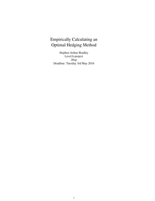
  • 7. 2.2.1 Volatility Smile What is interesting about the implied volatility is how it changes with the strike price, i.e. how the implied volatility changes depending on how in-the-money or out-of-the-money the option is. An option is called in-the-money if exercising it at the current time would generate a profit and out-of-the-money if exercising the option would generate a loss. This relationship is shown in Figure 1. Exercise Price 18 20 22 24 26 28 30 32 34 36 38 ImpliedVolatility 0 0.1 0.2 0.3 0.4 0.5 0.6 0.7 0.8 0.9 1 Volatility Smile for selected call options Figure 1: Volatility smile for a section of the data; i.e. the strike price against the implied volatility for all options which become available on the 24th of April 2014 and which expire on the 30th of May 2014. Where the vertical line represents the current stock price (the price of the stock on 24th of April) This Figure shows that there is a clear relationship; the volatility seems to be an almost symmetrical, gradually increasing function of the difference between the strike price and the current stock price. There is a subtle problem with this pattern because the current price is not in the centre of the curve. However, the ”current” stock price process we have access to was recorded at the end of each trading day, and the closing hours of a trading day are the most busy. This means that, the changing price process on each day of busy trading, has been approximated by a single value. Thus, although the process will be roughly representative of the true price process, we can expect small deviations from the most reasonable answers. In short, the current price line in Figure 1 indicates the last recorded value of the stock at the end of the day, but perhaps a more representative value for that day would have been in the centre of the curve. 2.3 Comparison of Implied and Historical Volatility The No-Arbitrage principle assures us that the volatility of an option will give the fair price, i.e. the price for which the expected overall profit will be zero. In reality however, the seller/writer of the option will be intending to make a profit, thus, the price will be a little higher than the fair market price. This means that the implied volatility and the realized (historical) volatility will take different values by design. Note that the price of an option is always an increasing function of the volatility as illustrated by Figure 2. Since the volatility is the only unobserved quantity, this figure 7
  • 8. shows that increasing the price of the option is identical to increasing the assumed value of volatility. Hence, by increasing the price of an option above the fair market price, the writer of the option has increased their implied volatility. This suggests that implied volatility will always exceed the true volatility of the market. Since the historical volatility is an unbiased estimate of the true volatility, we would expect the seller of the option to make a profit if the implied volatility exceeds the historical volatility. This implies that the seller is expected to loose money when their implied volatility is lower than the current historical volatility. Equivalently, this situation yields an expected profit for the buyer and this will effectively be arbitrage if the variance is sufficiently small. As we are hedging these options, we are assuming the role of the seller (taking a short position) so it is important to check this feature. The comparison is shown in Figure 21. 120 110 Stock Price 100 surface plot illustrating that the option price increases with volatility 90 800 0.2 Volatility 0.4 0.6 0.8 60 100 40 20 0 80 1 OptionPrice Figure 2: Black Scholes price for a call option with changing volatility and strike price Time (days) 20 40 60 80 100 volatility 0 0.5 1 1.5 2 2.5 3 3.5 4 Comparison of historical and implied volatility Implied Historical Time (days) 20 40 60 80 100 volatility 0 0.1 0.2 0.3 0.4 0.5 Comparison of historical and implied volatility Implied Historical Figure 3: Historical and Implied volatility for the dataset 8
  • 9. From Figure 3 we can see that very few options have an implied volatility below the estimates of realised volatility. From the above, this implies that the vast majority of these options will expect a positive return. This is an expected result and motivates the writing of options. 3 The Greeks Once we decide on a model for the volatility process and for the evolution of the stock price, we can then hedge the portfolio. However, there are various methods to choose from before in order to hedge an option. Each method depends on certain financial objects, known as Greeks. These objects are referred to as Greeks simply because most financial objects of this type are denoted by Greek letters, [8]. In this section we shall consider some of them and elaborate on some hedging methods. 3.1 Delta An option’s delta is the change in the price of the option for every unit change in the price of the underlying stock, i.e. an indication of the sensitivity of the option to the stock price. For example, if an option has a delta of 1 2 and the price of the underlying stock increases by x, the price of the option will increase by 1 2 x. Consider the effect of an increasing stock price on call and put options. The pay off of a call option is given by (ST − K)+ so every increase in St increases the expected pay off of the option. Under the assumptions of a fair market, the price of the option will then increase which indicates that call options have a positive delta. On the other hand, a put option has a pay off of (K − ST )+ whose expected value will decrease as the stock price increases. Under the same assumptions, the price of the option will decrease. Thus, put options have a negative delta. Furthermore, consider an in-the-money call option. Then, as time, t, approaches T (the expiration date) there will be a pay off of (ST − K)+ ≈ St − K and clearly this is linear in St so an increase of 1 in the stock price would increase the pay off by 1, and so, increase the option price by 1. This implies that the delta of a call option tends to 1 as t tends to T. Similarly, consider an in-the-money put option. The pay off of this option is (K−St)+ and will tend to K −St as t tends to T, thus, each unit increase in the stock price will result in a unit decrease in the option price. This shows that the delta of an in-the-money put option tends to -1 as t tends to T. 3.2 Delta Hedging As above, an option’s delta is equal to the change in value of the option per unit change in the underlying stock price. Thus, if we write (sell) an option and calculate it’s delta at present time to be δ, then we can hedge the option by shorting (selling) δ shares of the stock. After doing this, a unit increase in the stock will increase the option’s price by δ and will cause us to loose δ by shorting the stock, thus, the value of the portfolio will change by δ-δ=0. When this holds, we say that the portfolio is delta neutral. This shows that all risk has theoretically been eliminated and confirms the validity of the hedging method. However, the delta of an option is not constant, so the number of shares of the under- lying asset will need to be continually updated. This is a little impractical and in reality there will be transaction fees when buying/selling shares of the stock. For simplicity, in our calculations, we shall not consider transaction fees but, so that the results and conclusions are useful in a practical sense, we shall only implement the hedging method at the end of each day, i.e. we shall update the number of shares held in the portfolio once per day. 9
  • 10. 3.3 Gamma It is clear that the delta of an option will not be the only important quantity. In general, the value of the option cannot be expected to change as a linear function of the stock price. We can generalizing this method to also include the second derivative of the stock price process. An option’s gamma is a measure of the sensitivity of the delta to the stock price, the change in the value of delta per unit change in the stock price, which defines gamma as a second derivative risk [8]. If we consider delta as the speed the option price changes with respect to the stock price, then we can consider the gamma as the acceleration of the option price with respect to the stock price. Since gamma is a second derivative of an unobserved quantity, estimation of the value of gamma will be very difficult and more likely to be inaccurate - apart from in some simple cases. 3.4 Vega Similar to delta, an option’s vega, denoted ν, is the change in the option price per unit change in volatility. This method deals with a different type of risk. As we have seen in Figure 2, the volatility can have a strong impact on the value of an option. This suggests that an increase in the market volatility will increase the value of the option by increasing the expected profit. More specifically, if we were to write an option when the volatility was low then we would have to sell it at a low price but if the volatility increased then our potential losses would also increase. To hedge this type of risk and calculate a vega neutral position, we will need to buy a certain number of options. The number of options to buy will be a very difficult quantity to measure because it will depend sensitively on the volatility process, which is unobserved and estimated in a number of ways. 10
  • 11. 4 Black Scholes Model 4.1 Assumptions The assumptions under the Black Scholes Model are as follows. • Volatility of the stock, σ, is constant in time (this is the most important and controversial assumption) • No dividends are paid to the stock owner • The interest rate is a known constant, r • No transaction fees, so buying and selling stocks is free • Liquidity is such that any amount of any stock can be bought or sold at any time However, the model can be manipulated in order to be more useful in real life applications. For example, the constant volatility can simply be replaced by the implied volatility or by a stochastic volatility measure. 4.2 Black Scholes Equation The Black Scholes partial differential equation states the following. dS = S(µdt + σdW) where St denotes the price of a stock at time t, µ denotes the drift, σ denotes the stock’s volatility and Wt is a Brownian motion with distribution N(0, t). A solution to this equa- tion must take the form: St = Aeµt+σWt where A is a constant. Setting t=0 we can see that A must equal S0 (the initial value of the stock), i.e. St = S0eµt+σWt Let S∗ t denote the discounted pay off such that S∗ t = Ste−rt . Then we have: E(S∗ t ) =e−rt E(St) =e−rt E(S0eµt+σWt ) =S0e(µ−r)t E(eσWt ) =S0e(µ−r)t E(eN(0,σ2 t) ) =S0e(µ−r)t e σ2t 2 =S0e(µ−r+ σ2 2 )t Hence, when µ = (r − σ2 2 ), S∗ t will be a Martingale. This is a desired property to ensure that the stock price can be expressed as follows. St = S0e(r− σ2 2 )t+σWt 11
  • 12. 4.3 Option Pricing Here, we consider only European Call options, in which the call can only be exercised on the expiration date and not before. A European Put option can be calculated by first finding the price of the corresponding call option and invoking Put-Call Parity. Let K denote the strike price for the option, S0 denote the current stock price, T the time until expiration, and let r denote the fixed interest rate. Then the option price is calculated as follows. d1 := log(S0 K ) + T(r + σ2 2 ) σ √ T d2 := log(S0 K ) + T(r − σ2 2 ) σ √ T The price of the call option is given by: C(S0, T) = S0Φ(d1) − Ke−rT Φ(d2) and the price of the corresponding put option is: P(S0, T) = Ke−rT Φ(−d2) − SΦ(−d1) 4.4 Delta Calculation In order to implement a delta hedging technique we will need the ability to calculate delta for European options. Under the Black Scholes model, the delta of a call option is given by: Φ(d1) where Φ(-) represents the cumulative distribution function of a standard Normal random variable and d1 is as above, i.e. δ = Φ log(S0 K ) + T(r + σ2 2 ) σ √ T Similarly, for put options we have delta as Φ(d1). This is obvious from the above expressions for C(S0, T) and P(S0, T) when we recall that the delta is simply the differential of the option price with respect to the stock price, S0. Figure 4: Resulting profit from delta hedging the options using historical volatility and the Black Scholes model 4.5 Delta Hedging with Historical Volatility The first hedging method we shall implement is the Delta Hedging method under the Black Scholes model, with the volatility estimated by the historical volatility. From this point on, for simplicity, we shall assume that the interest rate, µ or r, is equal to zero. 12
  • 13. For each individual option in the available portfolio, the value of delta is calculated (under the Black Scholes assumptions) at the end of each day and the option is hedged accordingly. For a call option this corresponds to buying delta shares of the stock and for a put option this corresponds to selling (taken a short position) on delta shares of the stock at the current (end of day) price. In either case, the value of delta needs to be calculated in a different way. This hedging technique has been applied to all options which expire in at least 5 days and the options with a expiry of 4 or fewer days have not been hedged, this is again for practical purposes because we are assuming that it is not a profitable use of time to hedge an option which expires in only a few days. This is a reasonable and common approach. Figure 5: The time (in days) until expiry of those options with an absolute profit which is larger than 1.5 The histogram of resulting profit/loss, displayed in Figure 4, illustrates the consistency of the results and confirms that this method eliminates the vast majority of the risk involved in writing these options (as is the methods purpose). Most values are close to zero, as we would expect, and most are positive which is encouraging. This method is further supported by the histogram in Figure 5 which shows that almost all (1357/1403) of the options resulting in an extreme profit/loss, expire within less than 5 days of purchase (where an absolute value greater than 1.5 is classified as extreme, since 1.5 is the average price of an option). This means that they have not been hedged; for a practical approach as previously stated. Thus, the vast majority of the variance is due to options which were not hedged and this is a significant result because the options which were not hedged make up only 12.7% (3349/26388) of the total number of options. Since almost all the variance is due to a lack of hedging, it may be more useful to ex- plore the analysis of only the hedged options. The hedged options have a mean of 0.0512 and a standard deviation of 0·083. The value 0.0512 seems insignificant but it is close to zero by design (in minimising the risk we decrease the potential profits). Also, it is greater than zero and since the standard deviation is fairly small, this profit is consistent enough to effectively be called arbitrage. This mean is not as insignificant as it appears. The average profit is equal to 3.44% of the average option price which is an impressive degree of arbitrage. Thus, we must conclude that this method functions very well, in fact, this has shown a very promising result and suggests that we could enjoy significant improvement in our profits by relaxing our rule for practicality, i.e. hedging options of any expiry date. To decide if this would be best suited to our purposes, we shall now analyse the effects of the exhaustive approach more closely. 13
  • 14. Option (time ordered) #104 0 0.5 1 1.5 2 2.5 Profit -3 -2 -1 0 1 2 3 Historical volatility approach compared with no hedging method Figure 6: Contrast of the profit of hedging all options when using Black-Scholes and his- torical volatility (yellow) as opposed to not applying a hedge (blue) 4.5.1 Hedging All Options From Figure 7 we can see that abandoning our practical approach has significantly reduced the variance in the profits (from 0.4596 to 0.0080) but has also significantly reduced the potential profit. It is interesting that the median does not seem to have significantly changed (0.0154 from 0.0162) which suggests that there are roughly equal numbers of profits and losses in each case. This is expected because hedging methods are designed to eliminate risk and not to turn losses into profits or to maximize profits. An important consideration of hedging is that someone who is going to the trouble of hedging a portfolio, is likely to apply the method to a large number of options. This sug- gests that, assuming the standard deviation of profits is sufficiently low, the only important value is the mean profit. Here, we have that the mean profit has changed from 0.1229 to 0.0478. This is an extremely important result because, the average profit has been reduced to a third of its original size. Note that we are not suggesting the only important quantity is the mean. If we were to sell these options with no hedging method, the resulting profit would have mean 0.0601 but this does not imply that no hedging method at all is better than our historical volatility approach. This is clear from the graph in Figure 6 which clearly shows how the risk has been minimised. In practice, this is always an unwanted side effect when hedging a portfolio and can be seen as the cost of a safe, risk free portfolio. Figure 6 illustrates how hedging methods will 14
  • 15. control the risk and simultaneously limit the profits. The initial losses shown in the hedged options are likely to be largely caused by the temporarily high volatility in the underlying, shown by the extreme profits and losses of the ’unhedged’ options in blue. Since the short-term options generate a larger profit when they are not hedged, this idea of the importance of the mean suggests that the application of a hedging method is not the optimal decision when the option is only available for a small number of days. Also note that we have not included transaction fees in our model which would give further evidence to the practical approach. However, this approach, in a hedging framework, implies that the profit from these short-term options is not exposed to risk. This is a very bold assumption to make for any option since it contradicts the assumption of a free market; that there are no arbitrage opportunities. Nonetheless, we are searching for the most practical approach so we shall examine the evidence before discarding the method. Practical Hedge All Profit -2 0 2 4 6 8 10 12 Hedging with Black-Scholes and Historical volatility Figure 7: Box diagrams comparing the practical method to the method of hedging all options, when using Black-Scholes and historical volatility We could argue that these profits are unaffected by risk if they are consistently positive and are independent of the market. Figure 8 shows a close up of the histogram of profits (short-term options only) when we do not hedge. This suggests that there is still risk in- volved because a reasonable number are ending in a loss. However, the histogram is a little misleading because the bar between −0.02 and 0.04 consists of over 2200 options. Thus, these options are very consistent but this level of consistency doesn’t imply risk free. To decide whether the series depends on the market behaviour we would like to know if the price process is correlated with the profits from the short-term options. We can cal- culate the mean profit from these options, daily, and compute the cross correlation between the price process, and this sequence of mean profits. This cross correlation is plotted in 15
  • 16. Profit with no hedge -1.5 -1 -0.5 0 0.5 1 1.5 2 Frequency 0 10 20 30 40 50 60 70 80 90 100 Histogram of unhedged, short-term options Figure 8: Histogram showing the profit from short-term options (under 5 days) when un- hedged. Figure 9 using a rough indication of significance which relies on a null hypothesis that the true correlations are zero with a variance of 1/sqrt112, since 112 is the length of this time series. The Figure shows that the market behaviour (represented by the price process of the stock) appears to be weakly correlated with these average profits. Lag, in the Figure, is referring to the price process, e.g. at lag K, we are examining the expectation: E( [Xt−K − ¯X] · [Pt − ¯P] ) E( [Xt − ¯X]2) · E([Pt − ¯P]2 ) where X,P represent the price process and profit process respectively. The most important feature of the cross correlation, is that there is a significant negative correlation for negative lags. Although the correlation is only briefly significant, this is extremely important because it shows that the past of the market behaviour is correlated with the present profits. This implies that the profits from these options depend on market behaviour and so, cannot be considered as risk free arbitrage opportunities. In a hedging framework, minimizing risk is the most important goal, thus, the most sensible thing to do here is to be cautious and assume that the correlation is significant. To conclude this section, we shall surrender our practical approach of only hedging certain options. Instead, we shall exchange potential profits for security, and hedge all available options. 16
  • 17. Lag -100 -80 -60 -40 -20 0 20 40 60 80 100 Correlation -0.25 -0.2 -0.15 -0.1 -0.05 0 0.05 0.1 0.15 0.2 Cross correlation between the price process and the average daily profit from short-term options Figure 9: Cross correlation of the observed price process with the series of daily mean profits from short-term options. 4.6 Delta Hedging with Implied Volatility This method has been calculated in the same way as the previous method but with an implied volatility instead of the historical volatility. It seems reasonable to expect that this method will perform better than the previous method purely due to the increased flexibility of the implied volatility. From our previous conclusion, we shall now consider hedging all options in the portfo- lio; in order to make a fair comparison. Since we have shown that a simple histogram can be misleading, we shall consider a comparison similar to that of Figure 6. This comparison is shown in Figure 10. 4.7 Comparison of the Performance of Implied and Historical models Figure 10 shows a very similar structure to that of Figure 6 but contains some subtle differ- ences. Firstly, the initial options generate a significant loss under historical volatility, due to the previously mentioned reasons, but under implied volatility we do not incur such losses. The difference here is entirely due to the independence structure of the volatility process. We calculate each value of implied volatility from the market data at that time as opposed to accumulating a large amount of data to sufficiently estimate its value under a historical model. Another difference is that many of the profits are greater than those under the historical volatility model. This is not obvious from Figure 10 so we shall use a different visualiza- tion. Collecting all options which are available for an identical number of days, we can much more easily observe and compare the effects of historical and implied volatility un- der the Black-Scholes model. This plot is shown in Figure 11. This plot shows that under implied volatility, the generated profit is almost always greater. 17
  • 18. Option (time ordered) #104 0 0.5 1 1.5 2 2.5 Profit -3 -2 -1 0 1 2 3 Implied volatility approach compared with no hedging method Figure 10: Contrast of the profit of hedging all options when using Black-Scholes and implied volatility (yellow) as opposed to not applying a hedge (blue). To explore whether this method has out performed the historical volatility model we shall examine the statistics. model variance mean Historical 0.0095 0.0478 Implied 0.0181 0.0666 Firstly, the mean is greater under the implied volatility model, as expected from Figure 11. More interestingly however, the variance of the generated profits has more than dou- bled. We could argue, as before, that both variances are very low so the only meaningful comparison is that of the mean but this would be a minimalist approach. Comparing these outputs using box diagrams, in Figure 12, indicates the distribution of profits. It is obvious that the increased variance is caused by an increase in the number of pos- itive ’outliers’, i.e. values exceeding the 75th percentile of the data. This is clearly visible from the diagram because the outliers (red crosses) in the positive y-axis, referring to posi- tive profit, have become much more dense. This increased number of larger profits will be responsible for the increased mean. However, there has also been an increase in the number of negative outliers which is indicated by the density of the negative outliers. This feature of rough symmetry implies that the profits gained have been at the expense of risk. In our calculations, the implied volatility of each option has been independent of all previous data. This feature is largely responsible for the models success but could also be considered as a problem in some cases. 18
  • 19. Number of days from availability until expiry 0 5 10 15 20 25 30 35 40 45 50 Profits 0 10 20 30 40 50 60 70 80 90 Profit per length of availability under Historical and Implied volatility Figure 11: Comparison of the profits under implied and historical volatility using bins of identical lengths (in days) of availability When fitting a model, sometimes we observe a strange, unexpected change in the pa- rameters, e.g. in the fitted value of volatility, which seems like an anomaly when compared to previous patterns. Under a historical volatility model, we assume that the volatility is constant, which implies that all data are equally important and so, estimates which seem extreme will borrow strength from all previous data, i.e. more extreme values would be stabilized via a running mean with all previous values. When we have a sufficient amount of data, this would effectively bury the anomaly without the need for extra effort. The prob- lem is that these extreme values cannot be corrected or buried under the implied volatility model. The flexibility of a model to allow for a time-dependent volatility is very attractive and has proved very powerful. Thus, we shall maintain the assumption that the volatility is time-dependent. However, in order to include this idea in a model, we shall consider a consistent proba- bility structure for the volatility. This can be done under the Heston model. 19
  • 20. Historical Implied Profit -0.6 -0.4 -0.2 0 0.2 0.4 0.6 0.8 1 1.2 Profits under historical and implied volatility models Figure 12: Box diagrams comparing the resulting profits when using the Black-Scholes model with historical volatility and with implied volatility. 5 Heston Model This model takes a different approach to volatility. Previously, we have allowed volatility to be non-constant via considering the implied volatility to allow more flexibility in the model. Volatilities calculated in this way will not depend on one-another, and so, the volatility process could change sharply at every step. Although volatility represents randomness in the price process, the volatility process itself should admit some form of structure and a totally random, independent structure does not seem very justifiable. Here we shall allow for a volatility structure which evolves slowly through time. This model is not as widely implemented as Black-Scholes because it is more complex; this is due to the added complication of the stochastic volatility as opposed to the very simple idea of a constant one. The model is defined by the differential equations shown below. dSt = µStdt + σtStdW (1) t (1) dvt = −γ(vt − θ)dt + κ √ vtdW (2) t (2) dW (2) t = pdW (1) t + 1 − p2dW (3) t (3) Where the parameters are defined as follows; S represents the stock price process µ is the drift parameter, representing the interest rate 20
  • 21. σ is the time dependent volatility v is the variance, i.e. vt = σ2 t for convenience, since a solution to equation (1) depends only on σ2 t , and not σt θ is the long run mean of v γ is the rate of relaxation to this mean κ is the ’variance noise’ W(1) and W(2) are correlated 1-dimensional Brownian Motions p is the degree of correlation between W(1) and W(2) , as enforced by equation (3) in which W(3) is another standard Brownian Motion independent of W(1) and W(2) [1]. 5.1 The Feller Condition Here is a short and simple result worth mentioning. The Feller condition states that: 2γθ > κ ⇒ the process vt is strictly positive From the formula alone it is clear that this is a necessary result because the square root of vt (i.e. σt) is used and appears in Formula (1). Also, from the concept of volatility (behaving similarly to a standard deviation) we understand that negative values would not be intuitively meaningful. This is an extremely important feature of the model and can act as a quick check for the validity of fitted/assumed parameters. Alternatively, this con- dition could be written as a constraint in a constrained optimisation problem, as we shall implement in our model calibration. 5.2 Euler-Maruyama Method The Heston model is not as commonly used as Black Scholes due to it’s increased com- plexity and the computational cost of it’s application, for example, there is no closed form expression for the price of an option under the Heston model. Thus, we will need a way to simulate the the evolution of the price process and estimate the price of the option. As mentioned above, we shall simplify this model by setting the interest rate, µ, equal to zero. This gives: dSt = √ vtStdW (1) t (4) dvt = −γ(vt − θ)dt + κ √ vtdW (2) t (5) Thus, assuming these parameters are known, a simultaneous realisation of {St}t>0 and {vt}t>0 can be simulated using the Euler-Maruyama Method [7]. The Euler-Maruyama Method is used to simulate stochastic processes from stochastic differential equations (SDE’s). The application of this algorithm is explained below. 1. replace dSt and dvt with S (t + 1) − S (t) and v (t + 1) − v (t), respectively 2. replace dt with 1 252 to annualize (there are 252 business days per year) 3. make S (t + 1) and v (t + 1) the subjects of the equations 4. generate the process iteratively from equations 4 and 5 This results in equations: S (t + 1) = S (t) + v (t)S (t) (1) t v (t + 1) = v (t) − γ [v (t) − θ] 1 252 + κ v (t) p (1) t + 1 − p2 (2) t 21
  • 22. where S(0) refers to the current stock price, v(0) refers to the current volatility and (1) t , (2) t are independent, Gaussian noise processes with mean zero and variance 1 252 ; since the length of the interval is 1 252 in years (considering only trading days). Note that S(0) is known and v(0) can be estimated by the current market volatility (current estimate of historical volatility). Assuming that the parameters are known (or estimated/fitted), we can use the Euler- Maruyama method above to simulate the future of the process. Further, the hypothetical profit can be calculated for each simulation and an average should be roughly equal to the expectation of the resulting profit; by the weak law of large numbers under the assumption that the parameters are adequately estimated. That is to say, we can use this algorithm to give good estimates of E(ST − K)+ and E(K − ST )+ for call and put options respectively. By the assumption of a fair market, this expectation will be equal to the fair price of the option at the present time. Then we could calculate a delta hedge for the options from the following formula: ∆(St) = lim →0 C(St + ) − C(St) (6) and we can approximate this by taking a very small . Clearly this will be very sensitive to errors in the price of the option so we will have to decide on a reasonable number of iterations in order to balance this crucial issue of accuracy with computational efficiency. This issue is especially important because we are considering a large portfolio of over 26,000 options which means that the algorithm will have to run over 26,000 times. Ultimately, however, the focus will be on accuracy and the algorithm will be required to perform an extremely large number of calculations. Such a problem makes this method rather impractical. 5.3 Fast Fourier Transform The Fast Fourier Transform (FFT) is a powerful solution to this problem of efficiency. The FFT significantly reduces this computational cost and makes the model much more attractive and is likely to be the main cause for the popularity of the Heston model. Take f(·) as the density function of the log-return of the underlying price process, then (subject to the assumption that f is an integrable function) the Fourier transform of f is given by: F(φ) = +∞ −∞ eiφx f(x)dx f(x) = 1 2π +∞ −∞ e−iφz F(φ)dφ where F is the characteristic function of f, [3]. The FFT method is very practical in calculating summations of of the form: n h=1 ei 2π n (h−1)(k−1) g(h) (7) for some function g(·), [3]. This is useful to us because the fair price of a call option is given by: 22
  • 23. C(St) =E (ST − K)+ = +∞ −∞ (ST − K)+ f(log[ST ])d(log[ST ]) = +∞ log(K) (ST − K)f(log[ST ])d(log[ST ]) = +∞ log(K) (elog[ST ] − elog[K] )f(log[ST ])d(log[ST ]) = +∞ log(K) (exT − elog[K] )f(xT )dxT which can be efficiently approximated by a sum in the same form as (7). After some extensive calculus, Moodley [3] gives us the following form of the charac- teristic function, under the Heston model. CT (ku) ≈ e−αku π N j=1 e− 2π N (j−1)(u−1) eibvj FCT (vj) η 3 (3 + (−1)j − δj−1) The value of delta will need to be estimated here and will be very sensitive to changes/errors in the price of the option; this approximation of the call price will clearly need to be very accurate. Although this method suggests that estimates will be calculated extremely quickly, we must question whether this method is appropriate here. FFT methods are very useful in sig- nal processing because they will determine which frequencies are present in the time series and the amplitude of each frequency, [2]. This has many applications but in order to apply it here, we must assume that the daily stock prices can be decomposed into sinusoids of different frequencies. It is not clear if this assumption makes sense due to the unpredictable nature of the stock market. An attempt at a justification may be that the stock price is so unpredictable that we can treat it as a highly noisy process composed of many different frequencies of noise but this is not an intuitively sound justification. 23
  • 24. 5.4 Model Calibration In order to calculate a hedge as before, we must calculate the value of delta. To perform this calculation, we require the parameters of the Heston model. Thus, the parameters of the Heston model will need to be estimated from the data, i.e. calibrated to the data. For each day, we can use a simple method to fit the parameters on that day. Under our current assumptions, the parameters (i.e. γ, θ, κ, p) are constant in time so it seems contradictory to make separate estimates each day but this will help us to see if their structure is consistent and to test our assumptions. All parameters for a given day are calibrated to the options which become available on that day. A simple calibration method is to take the set of parameters (along with a value for the instantaneous volatility) for which the estimated option value is closest to the observed option prices. That is to say, on a day where n options become available, we will take the parameters, φ, that minimise: n i=1 [Observed option price − FFT(φ)]2 where FFT is a function to estimate the value under the Heston model. These fitted param- eters are shown in Figure 13. Days (2nd Jan - 5th June, 2014) 0 10 20 30 40 50 60 70 80 90 100 Parametervalue 0 0.5 1 1.5 2 2.5 3 3.5 4 4.5 5 Fitted Heston Parameters instantaneous volatility rate of relaxation (gamma) long run mean (theta) volatility of volatility (kappa) correlation (p) Figure 13: Calculated daily parameter values for the Heston model On the whole, the Figure seems to clarify that this fitting technique is sufficient because each curve has such a consistent structure. The only problem with this consistency is the sharp spikes, which appear in all model parameters (γ, θ, κ and p) in a synchronized way at about three different days; this is not a disaster because there is a total of 107 days in which options become available. These unexpected jumps in all model parameters do not appear in the estimate of the instantaneous volatility. This suggests that the spikes could not have been caused by some 24
  • 25. news or event involving the underlying stock. To elaborate further, these discontinuities occur on the following dates: 28-Jan, 19-May and 05-Jun. Usually we would associate such jumps in volatility structure with the anticipation of an event. For example, in the lead up to an earnings announcement we can expect the (implied) volatility to rise because the writers of the options want to limit the potential risk in case the earnings announcement has a significant impact on the market. However, these announcements for the first and second quarter occurred on April 17th and July 18th. So we can expect some other news, maybe news which is indirectly related to this stock, to be the cause of this if it is not simply an error in our calibration. For this reason, we shall consider sharp changes as an error in model fitting; it is not unreasonable to expect some anomalous results here since our method was so minimal. Formally, we shall use the following condition. If the estimate of a parameter, on day m, has increases by 100% of its original value, on day m − 1, then we shall say that the estimate for day m is an anomaly and we shall replace its value with the original estimate from day m − 1. Removing each anomaly in this way results in the estimates to the left of Figure 14 which are arguably more reliable. Days 0 20 40 60 80 100 120 0.1 0.2 0.3 0.4 0.5 0.6 0.7 0.8 0.9 Parameters with each anomaly removed Days 0 20 40 60 80 100 120 0.1 0.2 0.3 0.4 0.5 0.6 0.7 0.8 0.9 Smoothed Parameters gamma theta kappa p Figure 14: The graph to the left shows the daily estimates of the Heston parameters with each anomaly removed, and the graph to the right shows the smoothed parameters, i.e. a running mean of the estimates. Defining an anomaly in this way does not seem to have completely solved the problem for parameter theta since we still see some spikes, especially towards the end. However, the estimated value of theta does appear to gradually increase towards the end so it seems that the difference is systematic rather than an anomaly. An evolving structure would contradict our model assumptions but this gradual change does not seem significant enough to stop our model from being effective. Considering that the structure of each parameter is assumed to be constant, we can go a step further and smooth the daily estimates for the parameters using their running mean (mean of all previous estimates). This method results in the estimates on the right of Figure 14. These look convincing and we will use both sets of parameters to compare hedge performance. 25
  • 26. 5.5 Hedging with the Fast Fourier Transform For each set of parameters we can use the FFT to quickly estimate the price of the call option and we can use put call parity to calculate an estimate of the value of a put option. This seems to give a few strange mistakes when the option is only available for a small number of days, e.g. sometimes estimates a negative value for the option. This could be corrected by hedging the options until there is only a small number of days remaining, although, we have illustrated the importance of hedging every option at all times in section 4.5.1, so we shall not leave any options unhedged. 5.6 Hedging with Euler-Maruyama Simulation Although fairly impractical, the Euler-Maruyama method allows us to perform a simple procedure which will not experience strange errors; given a sufficient number of simul- taneously simulated chains with a sufficiently small value of in our approximation to formula 6. At each point, I have chosen to run 1,000 parallel simulations with 100 iterations in order to estimate each option price. Then Formula 6 (Euler Maruyama equations) can be used with a small value for epsilon, I have chosen 0.0001, to estimate the value of delta. This algorithm has taken multiple hours to compute and has not proved very practical. 6 GARCH model The Generalized Auto-Regressive Conditional Heteroskedasticity (ARCH) model with pa- rameter q is defined by the equations below. yt = log(St/St−1) = σt t σ2 t = ω + q i=1 αiσ2 t−i + p j=1 βiy2 t−j where St denotes the stock process, σt denotes the volatility process and t is a white noise process with mean zero and variance one. The GARCH model is termed: a conditional variance model, this comes from the feature below. σ2 t+1 = ω + q i=1 αiσ2 t+1−i + p j=1 βiy2 t+1−j (8) Notice that no estimation needs to take place here because all errors in this sum have been observed, so this will be the true value and not an estimate. In other words, condi- tional on the past and present data, the subsequent value of the volatility is known. The features discussed below are present in the returns, St − St−1, and the relative returns, St−St−1 St−1 , but we will apply the model to the log returns because this will allow a useful additivity feature: K t=1 yt = K t=1 log(St/St−1) = K t=1 log(St) − log(St−1) = log(SK) − log(S0) This alteration is for convenience but does not cause any problems in the model fitting because the log returns are roughly equal to the relative returns [5]. This is shown below via the Taylor expansion of the log function. 26
  • 27. log(St/St−1) = log 1 + St − St−1 St−1 = St − St−1 St−1 − St − St−1 St−1 2 + St − St−1 St−1 3 − ... ≈ St − St−1 St−1 This approximation holds in practice because the returns tend to be very small in com- parison to the stock price. 6.1 Model Features One feature which most models don’t explain well is how the volatility process in a finan- cial market tends to form clusters of high and low values. This feature is inherent from the way that investors tend to make decisions based on their feelings and predictions. All investors’ feelings and predictions are heavily influenced by news and current events and everyone views a similar version of that information. Thus, most investors decisions are strongly correlated and this has a strong effect on the volatility process, i.e. there will be some periods of low activity and some periods of high activity. Standard Normal Quantiles -3 -2 -1 0 1 2 3 QuantilesofInputSample -0.8 -0.6 -0.4 -0.2 0 0.2 0.4 0.6 0.8 1 1.2 QQ Plot of Sample Data versus Standard Normal Figure 15: Quantile plot of the log returns. Under the GARCH model we define the hidden volatility process using some Auto- Regressive terms, αi, which implies that the volatility process will be strongly dependent on recent values. This will lead to observed clusters of volatility as the structure of the process slowly changes [5]. Due to these clusters of volatilities, many financial data sets will have very heavy tails when compared to a normal distribution, [5]. Under a normal distribution, the probability of an extreme (high or low) value is very small, but when we see clusters of high volatility, the probability of these large values will increase. This will result in more extreme values than expected under a normal distribution, making the tails heavy in comparison. This 27
  • 28. feature is visible in the log returns of the data in Figure 15, where the quantile plot of the data is shown against that of the standard normal quantiles. Another feature we tend to observe in many financial time series is, a very low level of correlation with the past of the price process but a consistent correlation with the square of the past values. That is, the sample autocorrelations are small and are only significant for one or two lags, whereas, the autocorrelations for the series of squared values are non- decaying, [5]. To see if this is the case under the GARCH model, we can simply calculate the autocor- relation at different lags, as follows. The autocorrelation function is a normalized version of the auto covariance function so we will first need to calculate the expectation. E(yt) = E(σt t) = E(E(σt t)|Ft−1) by the Tower law = E(σtE( t)|Ft−1) since σt|Ft−1 is known, from (8) = E(σtE( t)) since t is independent of the past = 0 since E( t) = 0 where Ft denotes the filtration adapted to the process y at time t, i.e. the set containing all information up until time t. Lag -200 -150 -100 -50 0 50 100 150 200 correlation -0.2 0 0.2 0.4 0.6 0.8 1 Autocorrelation of a simulated GARCH process Figure 16: Figure showing the autocorrelations (blue) of the simulated GARCH(1,1) pro- cess, with parameters 0.98 and 0.01 respectively, along with the autocorrelations for the squared process (yellow). 28
  • 29. Lag -200 -150 -100 -50 0 50 100 150 200 correlation -0.2 0 0.2 0.4 0.6 0.8 1 Autocorrelation of the log returns log returns squared log returns Figure 17: Graph showing the autocorrelation of the observed price process and that of its squared values. Thus, using the same trick, we have the auto covariance function as follows, for k > 0. Cov(yt, yt+k) = E(yt · yt+k) − E(yt) · E(yt+k) = E(yt · yt+k) = E(σt t · σt+k t+k) = E(E(σt t · σt+k t+k)|Ft+k−1) = E(σt tσt+kE( t+k)|Ft+k−1) = E(σt tσt+kE( t+k)) = 0 So we can see that, due to the product with the white noise process, there is no correlation present. This means that the sample correlations will tend to be very low which is what we tend to observe. This is more evidence to support the use of a GARCH model for financial data. Furthermore, Figure 17 shows a non-decaying correlation with the squared values in the log returns of the price process and it is easy to see that the autocorrelations of the price process are decaying whereas those of the squared log returns are not. This is very similar to the autocorrelations which we observe in a realization of the GARCH model, e.g. that of a GARCH(1,1) model shown in Figure 16, i.e. this is another characteristic of observed data which GARCH models can take into account. A phenomenon which is very commonly observed, but poorly modelled, is the way that the volatility process reacts differently to certain movements of the price process, [5]. For instance, when the price process is dropping, its investors will all want to sell their shares and this will be observed as a spike in volatility or a cluster of large values in the volatility process. The GARCH model does not explain this behaviour because the volatility depends on the square of the log returns and not their sign. So it will be important to check that our data set doesn’t experience this feature in a significant way. Figure 18 shows a spread of values fairly close to the line y = x but consistently 29
  • 30. above it with a few outliers to the right; this shows that the volatility process is more likely to increase when the price process of the underlying drops. This may be a problem in the model because there is clearly a pattern emerging which the GARCH model will not explain. However, this low level of bias in the movements of the volatility may not be significant enough to impede the performance of the corresponding hedging method. We shall assume that this feature is not significant in our data and poses no problem to the application of the model; since there is no way to correct the GARCH model for this without considering the extension to an EGARCH model. We will not need to consider this extension if the GARCH model is not effected by this feature in a significant way. absolute value of the log return given that the stock price has risen 0 0.02 0.04 0.06 0.08 0.1 0.12 0.14 0.16 0.18 absolutevalueofthelogreturn giventhatthestockpricehasfallen 0 0.02 0.04 0.06 0.08 0.1 0.12 0.14 Reactions in the volatility to positive and negative movements Figure 18: Value of y2 after an increase in stock price plotted against the value of y2 after a drop in the stock price 6.2 Information Criterion The number of parameters to choose here is not clear, nor is there an analytical way of deciding on the best number. Instead, we take the simple approach of minimizing the information criterion. Increasing the number of parameters will always make the model more flexible and lead to an increased likelihood, regardless of whether we had already fitted the correct model [4]. Thus, if we were simply to maximize the likelihood, then we would continue adding parameters and many could be redundant. The information Criterion gives a value to each model which takes into account the maximum of the likelihood function under that model but also, a penalty for the number of parameters used. There are many ways that this penalty can be chosen and different penalty equations 30
  • 31. may lead to a different model choice. The most simple and widely used is the Akaike information criterion, its formula is given below. AIC = 2p − 2log(L) where L denotes the likelihood under this model and p denotes the number of parameters. In this case, 2p represents the penalty for the number of parameters and 2log(L) is the benefit of fitting a more flexible model. Balancing these quantities by minimising the AIC provides a simple method to calcu- late the number of parameters which best describes the observations. This method would make the algorithm more justifiable but more complicated and, as we shall discuss later, the simplicity of the model will significantly improve its running time. Especially since all the considered models must be fitted in order to compare their AIC value and this is much more time consuming than fitting a single model. To save time we shall set the number of parameters, p and q, equal to 15 and retain those which are significantly different from zero; this is done using t-statistics. This is a much less justified method but is intended to prioritise efficiency. Time (days from Jan 2004 to Dec 2014) 0 500 1000 1500 2000 2500 -0.15 -0.1 -0.05 0 0.05 0.1 0.15 0.2 Log returns of the stock price process Figure 19: Time series plot of the log returns of the price process. 6.3 Model Calibration The log returns of this series are shown in Figure 19 which illustrates how the volatility process has evolved through time. Although this model tends to explain large fluctuations in the volatility, the sections of the data which experience significantly larger levels of volatility will probably not be very informative about the near future. To be more specific, the data between 1000 and 1500 (Dec 2007 to Dec 2009) do not seem to be representative 31
  • 32. of the overall nature of the process or the most recent three years of data. This is obviously due to the financial crisis that occurred around July 2008. Thus, we shall only use data after this event to calibrate our model. Although we have found useful practical results in applying this method, we have done so assuming that the future estimates of the volatility process are the true values. This is a very bold assumption and will need to be justified, i.e. our confidence intervals for the estimates of σ2 will have to be sufficiently narrow. Time (Days) 0 200 400 600 800 1000 1200 Volatility #10-3 0 0.2 0.4 0.6 0.8 1 1.2 1.4 1.6 1.8 2 inferred conditional volatility upper and lower 95% confidence bounds Figure 20: Time series of the inferred conditional variance process with an estimated 95% confidence interval, estimated via 3 standard errors above the parameter estimates and 3 standard errors below. From Figure 20, we can see that the confidence intervals immediately become very wide. This is especially worrying because we are relying on some of these estimates 50 steps into the future. This has probably been caused by our quick method of setting the number of parameters equal to 15 via a rule of thumb without any justification. This is expected because it is likely that many of these 30 parameters are redundant, and as such, standard errors in estimation will be larger than usual. As discussed, taking more time to develop this algorithm and consider the information criterion would result in better model fitting, more appropriate forecasts and much narrower confidence intervals, at the expense of flexibility. Exploring this models features, we have concluded that the GARCH model would be appropriate for this dataset but this uncertainty in the parameters seems to suggest that the estimates will be poor and the risk may be increased. To decide if this is the case we shall compare the resulting profit with those of our other methods, i.e. these results cast 32
  • 33. suspicion over the suitability of this model but we shall apply the method and examine the results and statistics before reaching any firm conclusions. 6.4 Hedging with GARCH Now that we have a simple method of model fitting, we can predict the next value of the volatility process. Assuming that we have fitted the correct model, we have: To estimate all other future values of the volatility process, we shall simply replace the unobserved errors with their expectations in a recursive manner as shown below. For 1 < h ≤ p we have: ˆσ2 t+h = E  ω + q i=1 αiσ2 t+h−i + p j=1 βiy2 t+h−j   = ω + q i=1 αiˆσ2 t+h−i + p j=h βiy2 t+h−j + h−1 j=1 βi · E y2 t+h−j = ω + q i=1 αiˆσ2 t+h−i + p j=h βiy2 t+h−j + h−1 j=1 βiE σ2 t+h−j 2 t+h−j = ω + q i=1 αiˆσ2 t+h−i + p j=h βiy2 t+h−j + h−1 j=1 βiE(σ2 t+h−j)E( 2 t+h−j) = ω + q i=1 αiˆσ2 t+h−i + p j=h βiy2 t+h−j + h−1 j=1 βiˆσ2 t+h−j where ˆσn refers to its observed value if n ≤ t. Similarly, for h > p we have: ˆσ2 t+h = E  ω + q i=1 αiσ2 t+h−i + p j=1 βiy2 t+h−j   = ω + q i=1 αiˆσ2 t+h−i + p j=1 βi · E σ2 t+h−j 2 t+h−j = ω + q i=1 αiˆσ2 t+h−i + p j=1 βiˆσ2 t+h−j Now, note that the following telescopic sum gives: T n=t+1 yn = log(ST ) − log(ST −1) + log(ST −1) − log(ST −2) − ... + log(St+1) − log(St) = log(ST ) − log(St) = log(ST /St) Assuming the model is correct, we can calculate the future values of the volatility process σt and, via the independence of the white noise process, we have the following [5]. T n=t+1 yn ∼ N 0, T n=t+1 σ2 n 33
  • 34. We can now calculate the value of a call option using probability. E((ST − K)+ ) = St · E((ST /St − K/St)+ ) = St · E((exp(log(ST /St)) − K/St)+ ) To ease notation here we shall write Y to denote T n=t+1 yn and V to denote T n=t+1 σ2 n. E((ST − K)+ ) = St · E((exp(Y ) − K/St)+ ) = St · ∞ log(K/St) (exp(y) − K/St) · 1 √ 2πV exp −y2 2V dy = St · ∞ log(K/St) 1 √ 2πV exp −y2 2V + y dy − K ∞ log(K/St) 1 √ 2πV exp −y2 2V dy The second term here is simply the probability that a Normal(0, V ) random variable is greater than log(K/St). To calculate the first term we can complete the square as follows. −y2 2V + y = −1 2V (y2 − 2V y) = −1 2V (y − V )2 − V 2 = −1 2V (y − V )2 + V 2 Hence, the first term will simplify to: St · exp V 2 · Pr [N(V, V ) > log(K/St)] The fair price of the option is then given by the following result. E((ST−K)+ ) = St·exp V 2 ·Pr [N(V, V ) > log(K/St)]−K Pr[N(0, V ) > log(K/St)] This is an extremely practical result because this quantity, for estimated σ and fixed K is easily computed. Now that we have a simple formula for the option price, we can calculate the value of delta as follows. To directly calculate delta we must simply differentiate the expression for the fair price with respect to St. This is more simple than it appears because the differential of a prob- ability of this form is given as follows. Let f(·) denote the density function of a N(µ, V ) random variable and let F(·) denote its primitive. d dSt Pr(N(µ, V ) > log(K/St)) = d dSt ∞ log(K/St) f(x)dx = d dSt F(∞) − F(log(K/St)) = −f(log(K/St)) · d dSt log(K/St) = −f(log(K/St)) · (−1/St) = 1 St f(log(K/St)) = 1 St 1 √ 2πV exp −(log(K/St) − µ)2 /2V 34
  • 35. This formula is extremely useful but is only relevant for call options, we can use put call parity to calculate the delta for the corresponding put option as follows. Let δ denote the delta of the corresponding call option. d dS P(S, T) = d dS [C(S, T) − S + K] = d dS C(S, T) − 1 = δ − 1 Using this closed-form estimate for delta will improve the speed of the algorithm in comparison to previous methods. Throughout the application of this method we have pri- oritized speed and efficiency at the expense of accuracy, this is strongly indicated by the confidence intervals of Figure 20. These decisions are quite risky and cannot be easily justified except via the comparison of results. 35
  • 36. 7 Performance Comparison Firstly, we shall visually compare the results using box diagrams to give an impression of the number of profits and losses and an indication of the variance under each model. This is shown in Figure 21 where our applied methods are numbered as follows. 1. unhedged portfolio 2. Black Scholes model with Implied volatility 3. Black Scholes model with historical volatility 4. Heston model - Fast Fourier Transform 5. Heston model - Fast Fourier Transform with smoothed parameters 6. Heston model - Simulation 7. Heston model - Simulation with smoothed parameters 8. GARCH model 1 2 3 4 5 6 7 8 -10 -8 -6 -4 -2 0 2 4 6 8 10 Figure 21: Box diagrams of the resulting profit under each hedging method. From Figure 21, we can see that the simulations are largely increasing the variance of the profits. This is due to the estimates, at each step, for the value of delta. Estimating the wrong value for delta will result in our investing too much, or too little, in the stock. In doing this, we will not eliminate all of the risk and if we are very inaccurate in our estimate of delta we may significantly increase the risk as opposed to controlling it. This is the cause of the increased variance in our hedging methods. A solution here is clearly to increase the number of simulations and construct more accurate estimates but we are looking for a practical approach which could be applied each day, and this method has already proved quite impractical so we shall not consider it as viable choice. 36
  • 37. 7.1 Parameter Fitting Parameter fitting is the first important step to consider when hedging. The accuracy of the hedging method, i.e. the calculation of delta, tends to be very sensitive to the choice of fitted parameters. Since both Heston methods experience an increased variance, i.e. an increased risk, it would be fair to assume that there is a problem with the fitted parameters. To fit these parameters, we have minimized the squared difference of the available option prices with the corresponding price calculated by the Heston FFT function, within a specified margin of error. Problems may have arisen here because the FFT function is not sensitive to the parameters which are important in the evolution of the underlying process. 0.5 long run mean of the volatility (Theta) 0.4 Output of the FFT Function which was used to estimate our option prices 0.3 0.2 0.1 00 volatility of the volatility process (Kappa) 0.2 0.4 2.3045 2.305 2.3035 2.303 2.304 0.6 Callprice Figure 22: Estimated call price for different values of the parameters with all other param- eters held constant; current stock price=25, strike price=23, days until expiry=20, instanta- neous volatility=0.2, gamma=0.05, p=−0.01 For example, the daily movements of the volatility process (instantaneous volatility) will have a strong effect on the movements of the stock price and the evolution of the volatility process itself. These daily movements will be largely controlled by the mean and variance of the volatility process. Thus, our estimate of the mean and variance of the volatility process will be important in calculating any expectations. However, Figure 22 shows that, for some parameter values, the FFT function does not increase very quickly and in some sections it is fairly constant in terms of theta, as a result, many combinations of the values of theta and kappa will generate the same option price and our fitting method may not choose the most appropriate combination. Further, Figure 23 shows that, for some parameter values, the FFT function is not sig- nificantly effected by the value of kappa, suggesting that almost any arbitrary value could be assigned to kappa. The implications of this are going to be severe when we generate our estimates through simulation. A poor estimate of kappa alone could explain how poorly 37
  • 38. the simulations have performed. This may not be convincing because Figures 22 and 23 only describe two cases, but it is important to remember that the minimization algorithm ( lsqnonlin(·) ) will cycle through possible parameter combinations in the same way for each set of option data. This implies that, even when the parameters seem consistent, we may have been making systematic errors, which explains how our parameters are convincingly consistent yet potentially un- reliable. 1 Rate of relaxation to the mean (Gamma) 0.8 Output of the FFT Function which was used to estimate our option prices 0.6 0.4 0.2 00volatility of the volatility process (Kappa) 0.2 0.4 2.14 2.125 2.12 2.115 2.13 2.145 2.135 0.6 Callprice Figure 23: Estimated call price for different values of the parameters with all other param- eters held constant; current stock price=25, strike price=23, days until expiry=20, instanta- neous volatility=0.1, theta=0.1, p=−0.8 Interestingly, this problem of fitting appropriate parameters has caused the Black Sc- holes model to largely outperform the more flexible Heston model. This shows how a more complicated model does not necessarily give a better explanation of reality. In other words, the simple models seem to be more appropriate and much more easily applied. 7.2 Performance Statistics To reach an optimal choice, it will be very informative to compare the statistics of the profits under each method and, to emphasize practical importance, we shall also compare the time taken to run the algorithms. This data is shown in the table below, where Heston refers to the FFT method with smoothed parameters (since both FFT methods produce very similar results and the smoothed parameters are more justifiable). Also, we have seen that the Heston simulation method is useless in comparison to any other method so we do not need to compare its statistics. The hedging time refers to the time taken to hedge 101 options from the dataset; option 1000 to 1100, and the update time refers to the daily model fitting time which is calculated for the final day in the dataset. These values are not specifically important but are informative when considered purely for comparison. 38
  • 39. model mean mean as a % variance update time hedging time none 0.0601 57.34 0.2398 - - Historical 0.0478 52.15 0.0095 0.015806 0.281723 Implied 0.0666 58.48 0.0181 - 8.333090 Heston -0.5385 -10,215.49 12.4221 51.991874 9.990561 GARCH 0.0487 49.70 0.0112 1.280812 0.116998 GARCH (In) 0.0476 50.66 0.0081 1.267063 0.116513 The mean as a % column refers to the mean of the profit as a percentage of the option price and all times are measured in seconds. From these results, we can see that the Heston model is not useful and causes significant losses. This is more of a reflection of the difficulty in fitting the Heston model rather than the poor performance of the model itself. Furthermore, the time taken to calculate a hedging method is very important in practice and could arguably be the most important factor if the portfolio were large enough. Hence, even if the Heston model had been adequately fitted and managed to decrease the risk, this would not reduce the hedging time and a more sophisticated fitting method would only increase the time taken to fit the model. From this, we can conclude that the Heston model is not appropriate for our purposes and we shall not consider applying it any further. Considering the Black Scholes model, previously, it was not clear how to choose whether implied volatility had outperformed the historical volatility model. From the above table we can compare the time taken to apply each method and it seems that the historical volatility model will be much faster. However, one could consider the implied volatility model to be superior when the port- folio is very large because we can expect the variance to fall and become less important. On the other hand, as the portfolio gets larger, the time taken to apply the hedging technique will start to become a limiting factor due to time constraints in a practical sense. As such, the historical volatility model seems to be the optimal choice over the implied volatility. It is faster, more reliable and more risk-free than the implied volatility mode. This models high performance is likely due to its simplicity; the historical model is the simplest model possible. Simplicity is often an important factor affecting the model performance because more complex models do not necessarily yield a better explanation of the behaviour of pro- cesses in reality. The idea is that of Occam’s razor: ”The simplest answer is often correct” This is not always clear and is sometimes counter-intuitive when the model seems to be addressing real issues. The GARCH (In) model refers to the fitted GARCH model which forecasts using initial values. The difference is very important but is only noticeable in the variance of the profits. The subtle change here causes the GARCH model to generate the lowest of all variances, including the historical volatility model. This is a very meaningful result because the vari- ance gives us insight into the residual risk in the portfolio. Hence, we shall only consider GARCH models using the inferred conditional variances. Surprisingly, the GARCH model is even faster (per option) than the historical model and also takes an insignificant amount of time to calibrate each day. This speed and efficiency can be credited to the closed form solution of the delta calculation. Whereas, even the simplicity of the historical volatility model requires a calculation of the Black Scholes value for delta. It is unclear which features are important enough to be call a method optimal so we shall use a simple measure of performance. One way of choosing the optimal performance is to maximize the mean divided by the standard deviation. This would give the following values for the historical, implied and GARCH models respectively. 39
  • 40. mean standard deviation = 0.49042, 0.49503, 0.52889 This suggests that the GARCH model is clearly the optimal decision. In practice, we have shown the importance of time constraints so it would seem naive to neglect this feature of the performance of our models. To incorporate the importance of time we shall divide our measure of model performance by the hedging time. mean standard deviation · time = 1.7408, 0.059406, 4.5393 for historical, implied and GARCH respectively. We can conclude from this, that the GARCH model will be the best model suited to very large portfolios and outperforms all other methods by an impressive margin. Together, these results give strong evidence that the GARCH model will always be an optimal hedging model (when compared to the other methods we have considered here) whether time is considered as a constraint or not. This evidence could be explored further by considering and comparing different meth- ods of model calibration, i.e. applying the AIC to fit more appropriate models. Theoreti- cally, this will generate a more robust model but it will also damage the running time of the calibration algorithm. It is not clear which method would be more practically useful and we would have to compare distributions and statistics of profits, as above, in order to reach a more specific conclusion. We can conclude that the GARCH model is the optimal hedging method and further examination of parameter fitting (e.g. AIC) and model extensions (e.g. EGARCH) would give a more specific answer for our question of optimality. 40
  • 41. load y % option data load x % stock date and value data n=length(x); m=length(y); A Black Scholes Delta Hedging Code Historical volatility BS_profit_hist_all=1:m; for j=1:m i0=find(x(:,1)==y(j,1)); i9=find(x(:,1)==y(j,2)); hn=max(5,(i0-1)); hist_sigma=sqrt(var(diff(log( x(1:hn,5) )))*252); if y(j,4)==1 [c,˜]=blsprice(x(i0,5),y(j,3),0,(y(j,2)-y(j,1))/365,0.22); [cdelta,˜]=blsdelta(x(i0:i9-1,5),y(j,3),0,(y(j,2)-x(i0:i9-1,1))/365 ,hist_sigma); BS_profit_hist_all(j)=y(j,5)+sum(cdelta.*diff(x(i0:i9,5)))- subplus(x(i9,5)-y(j,3)); else [˜,p]=blsprice(x(i0,5),y(j,3),0,(y(j,2)-y(j,1))/365,0.22); [˜,pdelta]=blsdelta(x(i0:i9-1,5),y(j,3),0,(y(j,2)-x(i0:i9-1,1))/365, hist_sigma); BS_profit_hist_all(j)=y(j,5)+sum(pdelta.*diff(x(i0:i9,5)))- subplus(y(j,3)-x(i9,5)); end end Implied volatility BS_profit_imp_all=1:m; for j=1:m, i0=find(x(:,1)==y(j,1)); i9=find(x(:,1)==y(j,2)); if y(j,4)==1 imp_sigma=blsimpv(x(i0:i9-1,5),y(j,3),0,(y(j,2)-x(i0:i9-1,1))/365, y(j,5),10,0,0.000001,true); for mk=1:length(imp_sigma) if isnan(imp_sigma(mk)) imp_sigma(mk)=imp_sigma(find(isnan(imp_sigma)<1, 1, ’last’ )); end end [cdelta,˜]=blsdelta(x(i0:i9-1,5),y(j,3),0,(y(j,2)-x(i0:i9-1,1))/365, imp_sigma); BS_profit_imp_all(j)=y(j,5)+sum(cdelta.*diff(x(i0:i9,5)))- subplus(x(i9,5)-y(j,3)); else imp_sigma=blsimpv(x(i0:i9-1,5),y(j,3),0,(y(j,2)-x(i0:i9-1,1))/365, y(j,5),10,0,0.000001,false); for mk=1:length(imp_sigma) 41
  • 42. if isnan(imp_sigma(mk)) imp_sigma(mk)=imp_sigma(find(isnan(imp_sigma)<1, 1, ’last’ )); end end [˜,pdelta]=blsdelta(x(i0:i9-1,5),y(j,3),0,(y(j,2)-x(i0:i9-1,1))/365, imp_sigma); BS_profit_imp_all(j)=y(j,5)+sum(pdelta.*diff(x(i0:i9,5)))- subplus(y(j,3)-x(i9,5)); end end B Heston Delta Hedging Code FFT function function C=HestonCall(St,K,T,vt,kap,th,sig,rho,lda) %------------------------------------------------------------------------- %PURPOSE: computes the option price using Heston’s model. %-------------------------------------------------------------------------- %USAGE: C=HestonCall(St,K,r,sig,T,vt,kap,th,lda,rho) %-------------------------------------------------------------------------- %INPUT: St - scalar or vector, price of underlying at time t % K - scalar or vector, strike price % r - scalar or vector, continuously compound risk free rate expressed % as a positive decimal number. % sig- scalar or vector, volatility of the volatility of the % underlying(same time units as for r) % T - scalar or vector, time to maturity (same time units as for r) % vt - scalar or vector, instantaneous volatility % kap - scalar or vector, is the rate at which vt reverts to th % th - scalar or vector, is the long vol, or long run average price % volatility; as t tends to infinity, the expected value of volatility % lda - scalar or vector, risk premium for volatility % rho - scalar or vector, correlation between underlying and % volatility (rho<0 generates the leverage effect) %-------------------------------------------------------------------------- %OUTPUT: C - scalar or vector, Heston’s model call option price %-------------------------------------------------------------------------- dphi=0.01; maxphi=50; phi=(eps:dphi:maxphi)’; %f1 = CF_SVj(log(St),vt,T,r,kap*th,0.5,kap+lda-rho*sig,rho,sig,phi); %P1 = 0.5+(1/pi)*sum(real(exp(-i*phi*log(K)).*f1./(i*phi))*dphi); %f2 = CF_SVj(log(St),vt,T,r,kap*th,-0.5,kap+lda,rho,sig,phi); %P2 = 0.5+(1/pi)*sum(real(exp(-i*phi*log(K)).*f2./(i*phi))*dphi); %C = St*P1 -K*exp(-r*T)*P2; f1 = CF_SVj(log(St),vt,T,0,kap*th,0.5,kap+lda-rho*sig,rho,sig,phi); P1 = 0.5+(1/pi)*sum(real(exp(-1i*phi*log(K)).*f1./(1i*phi))*dphi); f2 = CF_SVj(log(St),vt,T,0,kap*th,-0.5,kap+lda,rho,sig,phi); P2 = 0.5+(1/pi)*sum(real(exp(-1i*phi*log(K)).*f2./(1i*phi))*dphi); C = St*P1 -K*exp(-0*T)*P2; Parameter Estimation using the FFT function. First, we calculate the implied volatility for each option. 42
  • 43. impv=(1:length(y)); for j=1:m, i0=find(x(:,1)==y(j,1)); i9=find(x(:,1)==y(j,2)); if y(j,4)==1 impv(j)=blsimpv(x(i0,5),y(j,3),0,(i9-i0)/365,y(j,5),10,0,0.000001,true); else impv(j)=blsimpv(x(i0,5),y(j,3),0,(i9-i0)/365,y(j,5),10,0,0.000001,false); end end Then we can calculate parameter estimates as follows. %Initial Parameter Guess for Hestion Model %V(1), Kappa, Theta, Vol of Volatility (sig), Correlation (rho) x0=[.5,.5,.5,.05,.5]; %Constraints (Lower and Upper bounds on Parameters) lb = [0, 0, 0, 0, -.9]; ub = [1, 100, 1, .5, .9]; % 107 is the latest date an option becomes available param=zeros(n,5); for d=1:n %Current Asset Price (Prompt Month Price) and Interest rate F0=x(d,5); dy=find(y(:,1)==x(d,1)); T=(y(dy,2)-y(dy,1))/365; strike=y(dy,3); impvol=impv(dy); CP=y(dy,4); %Optimization if isempty((find(y(:,1)==x(d,1)))) param(d,1:5) = [mean(param(1:(107),1)),mean(param(1:(107),2)), mean(param(1:(107),3)),mean(param(1:(107),4)),mean(param(1:(107),5))]; else param(d,1:5) = lsqnonlin(@costf2,x0,lb,ub); end end Removing every anomaly and smoothing the parameters uses the following code. param2=param; paramSmooth=param; for i=1:107 paramSmooth(i,2)=mean(param2(1:i,2)); paramSmooth(i,3)=mean(param2(1:i,3)); paramSmooth(i,4)=mean(param2(1:i,4)); paramSmooth(i,5)=mean(param2(1:i,5)); if i<252 for t=2:5 if param2(i+1,t)>2*param2(i,t) param2(i+1,t)=param2(i,t); 43
  • 44. end end end end for i=108:n paramSmooth(i,1:5)=[mean(param2(1:(107),1)),mean(param2(1:(107),2)), mean(param2(1:(107),3)),mean(param2(1:(107),4)),mean(param2(1:(107),5))]; end Heston Hedge using the FFT for j=1:m if mod(j,1000)==0 disp(j*100/m) end i0=find(x(:,1)==y(j,1)); i9=find(x(:,1)==y(j,2)); %V(1), Kappa (gamma for me), Theta, Vol of Volatility (sig), Correlation (rho) delt=i0:(i9-1); deltSm=i0:(i9-1); for h=i0:(i9-1) C=HestonCall(x(h,5),y(j,3),(i9-h)/365,paramSmooth(h,1),paramSmooth(h,2), paramSmooth(h,3),paramSmooth(h,4),paramSmooth(h,5),0); P=C+y(j,3)-x(h,5); Ceps=HestonCall(x(h,5)+epsilon,y(j,3),(i9-h)/365,paramSmooth(h,1), paramSmooth(h,2),paramSmooth(h,3),paramSmooth(h,4),paramSmooth(h,5),0); Peps=Ceps+y(j,3)-x(h,5)-epsilon; deltSm(h-i0+1)=y(j,4)*(Ceps-C)/epsilon+(1-y(j,4))*(Peps-P)/epsilon; %HestonCall(St,K,T,vt,kap,th,sig,rho,lda) C=HestonCall(x(h,5),y(j,3),(i9-h)/365,param(h,1),param(h,2), param(h,3),param(h,4),param(h,5),0); P=C+y(j,3)-x(h,5); Ceps=HestonCall(x(h,5)+epsilon,y(j,3),(i9-h)/365,param(h,1), param(h,2),param(h,3),param(h,4),param(h,5),0); Peps=Ceps+y(j,3)-x(h,5)-epsilon; delt(h-i0+1)=y(j,4)*(Ceps-C)/epsilon+(1-y(j,4))*(Peps-P)/epsilon; end % Delta(j)=y(j,4)*(Ceps-C)/epsilon+(1-y(j,4))*(Peps-P)/epsilon; % lda - scalar or vector, risk premium for volatility % rho - scalar or vector, correlation between underlying and % volatility (rho<0 generates the leverage effect) % blsdelta(x(i0:i9-1,5),y(j,3),0,(y(j,2)-x(i0:i9-1,1))/365,imp_sigma); Heston_profit(j)=y(j,5)-subplus(x(i9,5)-y(j,3))+delt*diff(x(i0:i9,5)); Heston_profitSm(j)=y(j,5)-subplus(x(i9,5)-y(j,3))+deltSm*diff(x(i0:i9,5)); end Heston Hedge using simulation epsilon=0.0001; Heston_Sim=1:m; Heston_SimSm=1:m; for j=1:m 44
  • 45. disp(j*100/m) if mod(j,1000)==0 save Heston_Sim Heston_Sim save Heston_SimSm Heston_SimSm end i0=find(x(:,1)==y(j,1)); i9=find(x(:,1)==y(j,2)); %V(1), Kappa (gamma for me), Theta, Vol of Volatility (sig), Correlation (rho) delt=i0:(i9-1); deltSm=i0:(i9-1); for h=i0:(i9-1) Cost=HestSim(x(h,5),y(j,3),(i9-h)/365,paramSmooth(h,1),paramSmooth(h,2), paramSmooth(h,3),paramSmooth(h,4),paramSmooth(h,5),y(j,4)); CostEps=HestSim(x(h,5)+epsilon,y(j,3),(i9-h)/365,paramSmooth(h,1), paramSmooth(h,2),paramSmooth(h,3),paramSmooth(h,4),paramSmooth(h,5),y(j,4)); deltSm(h-i0+1)=(CostEps-Cost)./epsilon; %HestonCall(St,K,T,vt,kap,th,sig,rho,lda) Cost=HestSim(x(h,5),y(j,3),(i9-h)/365,param(h,1),param(h,2), param(h,3),param(h,4),param(h,5),y(j,4)); CostEps=HestSim(x(h,5)+epsilon,y(j,3),(i9-h)/365,param(h,1), param(h,2),param(h,3),param(h,4),param(h,5),y(j,4)); delt(h-i0+1)=(CostEps-Cost)/epsilon; end % Delta(j)=y(j,4)*(Ceps-C)/epsilon+(1-y(j,4))*(Peps-P)/epsilon; % lda - scalar or vector, risk premium for volatility % rho - scalar or vector, correlation between underlying and % volatility (rho<0 generates the leverage effect) % blsdelta(x(i0:i9-1,5),y(j,3),0,(y(j,2)-x(i0:i9-1,1))/365,imp_sigma); Heston_Sim(j)=y(j,5)-subplus(x(i9,5)-y(j,3))+delt*diff(x(i0:i9,5)); Heston_SimSm(j)=y(j,5)-subplus(x(i9,5)-y(j,3))+deltSm*diff(x(i0:i9,5)); end C GARCH Delta Hedging Code This code uses the infer function to input the initial estimates of the volatility process. The method without is obviously the same but without the infered parameters, i.e. omitting this line of code. epsilon=0.0001; opts = optimset(’fmincon’); opts.Algorithm = ’interior-point’; forc=zeros(n,50); for h=2000:n X=x(1501:h,5); L=length(X); npar=15; model=estimate(garch(npar,npar),log(X(2:L)./X(1:(L-1))),’options’,opts); forc(h,1:50)=forecast(model,50,’Y0’,infer(model,log(X(2:L)./X(1:(L-1))))); disp(h*100/n) end 45
  • 46. save forc forc GARCHI=1:m; for j=1:m i0=find(x(:,1)==y(j,1)); i9=find(x(:,1)==y(j,2)); delt=i0:(i9-1); for h=i0:(i9-1) V=sum(forc(h,1:(i9-i0))); delt(h-i0+1)=exp(V/2)*(1-normcdf(log(y(j,3)/x(h,5)),V,sqrt(V)))+ exp(V/2)/(sqrt(2*pi*V))*exp(-(log(y(j,3)/x(h,5))-V)ˆ2/(2*V))- y(j,3)/(x(h,5)*sqrt(2*pi*V))*exp(-(log(y(j,3)/x(h,5)))ˆ2/(2*V))-1+y(j,4); end GARCHI(j)=y(j,5)-subplus(x(i9,5)-y(j,3))*y(j,4)- subplus(y(j,3)-x(i9,5))*(1-y(j,4))+delt*diff(x(i0:i9,5)); disp(j*100/m) end 46
  • 47. References [1] DRAGULESCU, A. A., AND YAKOVENKO, V. M. Probability distribution of returns in the heston model with stochastic volatility. Department of Physics (2002). url: http://arxiv.org/abs/cond-mat/0203046. [2] JAMES, J. F. A Student’s Guide to Fourier Transforms, third ed. Cambridge University Press, 2011. Cambridge Books Online. [3] MOODLEY, N. The heston model: A practical approach. Faculty of Science, University of the Witwatersrand, Johannesburg, South Africa. [4] POSADA, D., AND BUCKLEY, T. R. Model selection and model averaging in phy- logenetics: advantages of akaike information criterion and bayesian approaches over likelihood ratio tests. Systematic biology 53, 5 (2004), 793–808. [5] SIDOROV, SERGEI, D. P. B. V. Using news analytics data in garch mod- els. https://ideas.repec.org/a/ris/apltrx/0204.html, Applied Econometrics, Publishing House ”SINERGIA PRESS”, vol. 29(1), pages 82-96. [6] TORRICELLI, C., AND BRUNETTI, M. The put-call parity in the index options mar- kets: Further results for the italian mib30 options market. Department of Economics 0436, University of Modena and Reggio E., Faculty of Economics ”Marco Biagi”. [7] XUERONG MAO, A. T., AND YUAN, C. Euler-maruyama approximations in mean-reverting stochastic volatility model under regime-switching. Journal of Applied Mathematics and Stochastic Analysis (2006). vol. 2006, Article ID 80967,doi:10.1155/JAMSA/2006/80967, url: http://arxiv.org/abs/cond-mat/0203046. [8] ZASKODNY, PREMYSL, E. A. The Formulas for Ultima Greek. University of South Bohemia and University of Finance and Administration, Czech Republic, 2011. 47