Pricing and hedging of defaultable models

Technical report, IDE1141, August 25, 2011
Master’s Thesis in Financial Mathematics
Magdalena Antczak Marta Leniec
School of Information Science, Computer and Electrical Engineering
Halmstad University
Pricing and Hedging
of Defaultable Models

Pricing and Hedging
of Defaultable Models
Magdalena Antczak
Marta Leniec
Halmstad University
Project Report IDE1141
Master’s thesis in Financial Mathematics, 15 ECTS credits
Supervisor: Prof. Lioudmila Vostrikova-Jacod
Examiner: Prof. Ljudmila A. Bordag
External referees: Prof. Mikhail Babich
August 25, 2011
Department of Mathematics, Physics and Electrical engineering
School of Information Science, Computer and Electrical Engineering
Halmstad University

Preface
This thesis has been prepared at the University of Angers under the supervi-
sion of Professor Lioudmila Vostrikova-Jacod. We would like to thank her for
help in understanding the defaultable framework and useful remarks. The
conversations at the Faculty and seminars were priceless. We also want to
express our sincere gratitude to Professor Ljudmila Bordag for organizing
our Erasmus in France.

Abstract
Modelling defaultable contingent claims has attracted a lot of interest in
recent years, motivated in particular by the Late-2000s Financial Crisis.
In several papers various approaches on the subject have been made.
This thesis tries to summarize these results and derive explicit formu-
las for the prices of ﬁnancial derivatives with credit risk. It is divided
into two main parts. The ﬁrst one is devoted to the well-known theory
of modelling the default risk while the second one presents the results
concerning pricing of the defaultable models that we obtained ourselves.
iii

Contents
1 Introduction 1
2 Stochastic background 7
2.1 The probability space and filtrations . . . . . . . . . . . . . . 7
2.2 Stochastic processes . . . . . . . . . . . . . . . . . . . . . . . . 9
2.3 The Brownian filtration . . . . . . . . . . . . . . . . . . . . . 11
2.4 Stopping times . . . . . . . . . . . . . . . . . . . . . . . . . . 13
2.5 The Martingale Theory . . . . . . . . . . . . . . . . . . . . . . 14
3 The default setting 15
3.1 Basic assumptions . . . . . . . . . . . . . . . . . . . . . . . . . 15
3.2 The default process . . . . . . . . . . . . . . . . . . . . . . . . 16
4 The intensity-based approach in filtration H 19
4.1 The H-intensity of τ . . . . . . . . . . . . . . . . . . . . . . . 19
4.1.1 The intensity of default . . . . . . . . . . . . . . . . . . 19
4.1.2 The hazard function Γ . . . . . . . . . . . . . . . . . . 26
5 The Carthaginian enlargement of filtrations 33
5.1 Introduction . . . . . . . . . . . . . . . . . . . . . . . . . . . . 33
5.2 General projection tools . . . . . . . . . . . . . . . . . . . . . 34
5.3 Measurability properties in enlarged filtrations . . . . . . . . . 35
5.4 The E-hypothesis . . . . . . . . . . . . . . . . . . . . . . . . . 36
5.5 The change of measure on Gτ
. . . . . . . . . . . . . . . . . . 38
5.5.1 The survival process under measure P and P∗
. . . . . 42
6 The initial enlargement framework 43
6.1 Expectation tools . . . . . . . . . . . . . . . . . . . . . . . . . 44
6.2 The martingales characterization . . . . . . . . . . . . . . . . 45
6.3 The E-hypothesis and the absence of arbitrage in the filtration
Gτ
. . . . . . . . . . . . . . . . . . . . . . . . . . . . . . . . . 46
v

7 The progressive enlargement framework 47
7.1 The intensity approach . . . . . . . . . . . . . . . . . . . . . . 47
7.1.1 Expectation tools . . . . . . . . . . . . . . . . . . . . . 47
7.1.2 The F-hazard process (Γt)t≥0 . . . . . . . . . . . . . . 50
7.1.3 The G-intensity of τ . . . . . . . . . . . . . . . . . . . 52
7.1.4 H-hypothesis and the absence of arbitrage in the ﬁl-
tration G . . . . . . . . . . . . . . . . . . . . . . . . . 53
7.1.5 The value of information . . . . . . . . . . . . . . . . . 54
7.2 The density approach . . . . . . . . . . . . . . . . . . . . . . . 55
7.2.1 Projection tools . . . . . . . . . . . . . . . . . . . . . . 55
7.2.2 The H-hypothesis and special property of the condi-
tional density process . . . . . . . . . . . . . . . . . . . 56
7.2.3 The martingales characterization . . . . . . . . . . . . 57
8 Pricing and hedging of Black-Scholes type models with de-
fault 59
8.1 The model evaluation and the description of the task . . . . . 59
8.2 Methods of pricing in arbitrage-free and incomplete market . . 63
8.2.1 The arbitrage-free market . . . . . . . . . . . . . . . . 63
8.2.2 The incomplete market . . . . . . . . . . . . . . . . . . 63
8.2.3 The f-divergence minimization approach . . . . . . . . 63
8.2.4 The utility approach . . . . . . . . . . . . . . . . . . . 64
8.3 Martingale measures on Gτ
. . . . . . . . . . . . . . . . . . . 67
8.4 The distribution of τ with respect to P . . . . . . . . . . . . . 70
8.5 European call option pricing . . . . . . . . . . . . . . . . . . . 74
8.5.1 Pricing in the Black-Scholes market with default . . . . 75
8.5.2 The case when W(1)
and W(2)
are uncorrelated . . . . 76
8.5.3 The case when W(1)
and W(2)
are correlated with the
correlation coeﬃcient ρ . . . . . . . . . . . . . . . . . . 79
9 Conclusions 91
Notation 93
Notation 94
Bibliography 95
Appendix 96
vi

Chapter 1
Introduction
In the world of finance, it is crucial to consider the models based on the
fact that the companies may default. Hearing the word ’default’ one can
imagine the biggest defaults in the history of economy like that of Lehman
Brothers in 2008. However, the exact definition of a default explains it only
as a failure to meet debt obligations such as loans or bonds. The debtor
is in default when he is either unable or unwilling to pay the debt. One
has to distinguish the default from a state of being unable to pay the debts
precisely which is called insolvency. The company is insolvent when it is
unable to pay debts as they fall due (cash flow insolvency) or when the
liabilities exceed the assets (balance sheet insolvency). It is worth mentioning
that the insolvency can lead to a bankruptcy which is the process of legally
defining a financial situation as insolvent. While modelling credit risk, one
usually takes under consideration the company’s default in general, without
looking into the causes and hence distinguishing between being unable or
unwilling to pay the debts.
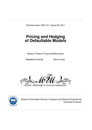
In the world of mathematics, the default appears as default time which is
a strictly positive random variable. One can define this random variable in
many ways. However, the most common one is the first time of crossing a
barrier by a certain process, e.g. a stock price process of a company (see a
Figure 9.1).
Modelling of the default event can be done in two manners. The first one is
called structural approach. It assumes that default time τ is a stopping time
in the assets filtration F. The second one, called reduced-form approach, is
based on the assumption that τ is a stopping time in a larger filtration and
may no longer be measurable with respect to the prices filtration. In our
thesis, we focus on the last approach.
1

2 Chapter 1. Introduction
Figure 1.1: An example of a defaultable company stock price process.
We consider a non-defaultable world which consists of riskless and risky
assets. A filtration generated by the prices of those assets is denoted by F
and called the reference filtration. It represents the information available
to the regular investor in a non-defaultable world. However, when we take
under consideration a possibility of a default we have to introduce default
time τ and create a defaultable framework which may consists of default-
free and defaultable assets, e.g. stock of the company that may default.
We have to study different types of information flows available to agents
trading in a defaultable market. On the one hand, the regular investors
add the information about default to F when it occurs, i.e. they work in
a progressive enlargement setting. On the other hand, we shall examine
also the insider, i.e. the agent who possesses information about default time
from the beginning. The information accessible to this agent is represented
by a filtration F initially enlarged by a positive random variable τ. In our
thesis, we explore the special theory which establishes methods of enlarging
the reference filtration by the additional information, namely Carthaginian
Enlargement of Filtrations (see [2]).
We distinguish two methods of modelling default time in a reduced-form
approach, namely the intensity (see [1]) and the conditional density-based

Pricing and Hedging of Defaultable Models 3
approach (see [2] and [3]). They are used to establish the expectation and
projection tools which are necessary for pricing an hedging of financial deriva-
tives. An intensity of default is simply a ratio of probability that default will
appear in a infinitely small time interval (under the condition that there
was no default before) and the time step. However, to determine the condi-
tional density of default, we need to assume that the conditional law of τ is
equivalent to the law of τ.
In the first chapter, we study some basic results concerning probability
spaces and filtrations, as well as stochastic processes, in particular a Brownian
motion. We introduce some facts concerning stopping times and martingales.
In the second chapter, we introduce crucial assumptions related to the
filtered probability space involving default time and all the price processes.
Then, we introduce the law of τ and we give a definition of a default process.
We determine the form of a random variable measurable with respect to
the σ-algebra generated by that process and give some properties of the
corresponding filtration.
Third chapter is devoted to the intensity approach in the filtration gen-
erated by the default process. In this framework, we give tools to compute
expectations with respect to the σ-algebra generated by this process. Then,
we value under the physical measure defaultable zero-coupon bond at time
t in the case of zero and non-zero spot rate for the agent whose information
flow is the filtration mentioned above. Finally, we give formulas and prop-
erties of the survival and hazard function and we represent once again the
defaultable zero-coupon bond value using these functions.
In the fourth chapter, we present firstly the theory of Carthaginian En-
largement of Filtrations and hence, the methods to enlarge reference filtra-
tion with an additional information. Secondly, we represent random variables
with respect to the corresponding σ-algebras. Then, we introduce the crucial
assumption that states that the conditional law of default time τ is equiv-
alent to the law of τ. In addition, we present the density hypothesis which
allows to express the distribution of τ conditioned on the information from
the reference filtration in terms of the conditional density process and the
law of τ. We show that under the additional assumption concerning the law
of τ, namely the property of being non-atomic, default time avoids stopping
times from the reference filtration. The second important part of this chap-
ter is devoted to introducing the so-called decoupling measure which makes

4 Chapter 1. Introduction
τ and the underlying risky assets independent. We consider some proper-
ties of the new measure and establish the expectation tools using obtained
independence. What is more, we establish the form of the survival process
under the physical and decoupling measure. Finally, we prove that initially
enlarged filtration inherits right-continuity from the reference filtration.
Fifth chapter presents some results obtained in the initially enlarged fil-
tration, i.e. the expectation tools and the characterization of martingales
from the enlarged filtration in terms of martingales from the reference filtra-
tion. We finish the chapter with establishing the conditions for the absence
of arbitrage in the enlarged filtration.
In the sixth chapter we examine the progressive enlargement framework.
We begin with the intensity-based approach and assume that a price process
follows the log-normal distribution and the reference filtration is generated
by a standard Brownian motion. Firstly, we establish some expectation tools.
Secondly, we introduce a hazard process in terms of the results obtained from
the expectation tools. Then, we introduce the intensity in the progressively
enlarged filtration. We continue the chapter by studying the hypothesis that
martingales from the reference filtration remain martingales in the enlarged
filtration, namely H-hypothesis which is strongly related to the absence of
arbitrage. We finish the intensity-based approach part with demonstrating
the value of the default information, i.e. the difference between the price of
a defaultable contingent claim for an agent who possesses the information
about the default when it occurs and the one who does not have this in-
formation. In the second part of this chapter, we analyse the density-based
approach. We begin with establishing the projection of random variables on
the progressively enlarged filtration and we obtain the Radon-Nikodým on
this filtration. We continue with examining the relation between the density
hypothesis and the H-hypothesis and finish with the martingales character-
ization.
The seventh chapter consists of our own results. We calculate the price
of the option written on a investment consisting of both, default-free and
defaultable assets. We consider a default-free market consisting of one risk-
less asset and one risky asset and a defaultable market created by adding
one defaultable asset to the preceding model. We define a reference filtra-
tion as a filtration generated by a price process of a default-free asset. We
define default time τ as the first time when defaultable asset’s price crosses
a certain barrier from interval (0, 1) and we establish distribution of τ. We

consider two agents trading in a defaultable market, a regular investor who
observes only a price process of a default-free asset and a special agent who
has additional information concerning default time τ from the beginning, i.e.
its distribution. We put an accent on the fact that the defaultable market is
arbitrage-free and incomplete for the regular investor and hence, we ﬁnd it
interesting to calculate the price of the option for such an investor. We ﬁnd a
pricing measure using the connection between two well-known methods, the
utility maximization and the f-divergence minimization.

Chapter 2
Stochastic background
In the Theory of Financial Markets pricing is based either on the stochastic
or partial differential equations approach. We will focus on the former one.
It is important to remind the most important definitions from the Theory of
Stochastic Processes which will be used throughout our thesis.
2.1 The probability space and filtrations
While considering the randomness, it is necessary to introduce a proba-
bility space (Ω, F, P) which is a mathematical form essential for modelling
the stock prices and default processes consisting of the states which occur
with uncertainty. A non-empty sample space Ω is an universe of all possi-
ble random events ω. In our case it is a space of all possible scenarios that
can happen on the financial market. For further calculations and reasoning
it is crucial to use a certain type of collections of these events ω ∈ Ω. Let
us denote P(Ω) the set of all subsets of Ω. From the Theory of Probabil-
ity we know how to treat the collections which are closed under countable
unions and joints. Consequently, we introduce the most important algebraic
structure, σ-algebra over Ω, as following.
Definition 2.1. Let Ω be a non-empty sample space. F ⊂ P(Ω) is called a
σ-algebra over Ω, if
i) ∅ ∈ F,
ii) F ∈ F ⇒ FC
∈ F,
iii) ∀i ∈ I, Fi ∈ F ⇒ i∈I Fi ∈ F, where I ⊂ N.
N is a set of natural numbers.
7

8 Chapter 2. Stochastic background
From the De Morgan’s laws we can easily combine ii) and iii) from the
previous definition and get that the countable joints remain in the σ-algebra.
Remark 2.1. If F is a σ-algebra over Ω, then
i) Ω ∈ F,
ii) ∀i ∈ I, Fi ∈ F ⇒ i∈I Fi ∈ F.
Through equipping the sample space with the σ-algebra F we get a pair
(Ω, F) called a measurable space. On such a space we can define a probability
measure and obtain the probability space.
Definition 2.2. Let Ω be a non-empty sample space and F a σ-algebra over
Ω. The pair (Ω, F) is called a measurable space.
In the Mathematical Finance, for pricing financial derivatives, one can use
several probability measures calculated from the actual market movements.
For instance, a martingale measure is based on the risk-neutrality approach.
Accordingly, in pursuance of the previous notations and assumptions we can
define a probability measure P on measurable space (Ω, F) defined on the
set of events from Ω.
Definition 2.3. We call a function P : F → [0, 1] a probability measure on
(Ω, F) if
i) P(∅) = 0,
ii) P(Ω) = 1,
iii) ∀i ∈ I Fi ∈ F are disjoint, i.e. Fi ∩ Fj = ∅ if i = j then
P(
i∈I
Fi) =
i∈I
P(Fi),
where I ⊂ N.
Broadly speaking, a probability space is a measurable space such that the
measure of the whole space is equal to one. In accordance with the previous
suppositions we can define it more formally.
Definition 2.4. We call a triplet (Ω, F, P) a probability space where Ω = ∅,
F is a σ-algebra over Ω and P is a probability measure on (Ω, F).
In mathematics there are some sets which can be ignored. In the Theory
of Probability we call them P-negligible sets. They can be omitted when
calculating integrals of measurable functions.

Definition 2.5. A set A ∈ F is called a P-negligible set if P(A) = 0.
In general, the probability space (Ω, F, P) does not have to contain all
P-negligible sets. However, it can be completed by incorporating all subsets
of P-negligible sets in a suitable manner.
Definition 2.6. A triplet (Ω, F, P) is called a complete probability space if
F contains all P-negligible sets.
It is important in the Theory of Martingales to define the filtration on
a measurable space (Ω, F). In the mathematical finance we understand the
filtration as the information available up to and including each time t which
is more and more precise as more data from the stock becomes accessible.
Definition 2.7. F is a filtration if F is a family of non-decreasing sub-σ-
algebras (PFt)t≥0 such that ∀t ≥ 0 Ft ⊂ F and ∀0 ≤ s < t < ∞ Fs ⊂ Ft.
Similarly as before, we define a filtered probability space (Ω, F, F, P) also
known as a stochastic basis or a probability space with a filtration of its
σ-algebra.
Definition 2.8. We call the quadruple (Ω, F, F, P) a filtered probability
space, where Ω = ∅, F is a σ-algebra over Ω, F is a filtration and P is a
probability measure.
For further considerations we introduce a complete filtered probability
space.
Definition 2.9. (Ω, F, F, P) a complete filtered probability space if F con-
tains all P-negligible sets and ∀t ≥ 0 F contains all P-negligible sets.
2.2 Stochastic processes
In the study of stochastic processes there is an important reason to include
σ-fields and filtrations because they are necessary to keep the track of the
information. The relating to time feature of stochastic processes implies the
flow of time. It means that at every moment t ≥ 0 we can talk about the
past, present and future as well as ask how much the observer of the process
knows about them at present. We can compare this information with how
much he knew in the past or will know in some certain time in the future.

In this chapter we give the definition of a stochastic process, a natural
filtration and we distinguish three types of measurability.
Definition 2.10. A stochastic process X = (Xt)t≥0 is a family of (Rd
, B(Rd
))-
valued random variables Xt, where ∀t ≥ 0 Xt is defined on the probability
space (Ω, F, P).
We will assume that d = 1 in further considerations.
Given the stochastic process X the most intuitive and the simplest way to
choose the filtration is to take the one generated by the stochastic process
itself.
Definition 2.11. A natural filtration FX
of a process X = (Xt)t≥0 is a
filtration
FX
= (FX
t )t≥0,
where
FX
t = σ(Xs, s ≤ t)
is the smallest σ-algebra with respect to which Xs is measurable for every
s ∈ [0, t].
One can interpret set A ∈ FX
t as follows. By the time t the observer
knows if the set A has occurred or not.
To avoid problems with the measurability in the Theory of Lebesgue
Integration, the probability measures are defined on σ-algebras and consid-
ered random variables are assumed to be measurable with respect to these
σ-algebras.
X is a function of two variables (t, ω) and it is convenient to have the
following definitions of the measurability.
Definition 2.12. The stochastic process X = (Xt)t≥0 is called B(R+) ⊗ F-
measurable if for every A ∈ B(R), the set
{(t, ω)|t ∈ R+, ω ∈ Ω : Xt(ω) ∈ A}
belongs to the product σ-algebra B(R+) ⊗ F.
One can be more precise and say that the stochastic process is B(R+)⊗F-
measurable if ∀t ≥ 0 the mapping
(t, ω) → Xt(ω) : (R+ × Ω, B(R+) ⊗ F) → (R, B(R))
is measurable.

The concept of measurability presented in the previous definition is rather
weak. Given the definition of the filtration we can define a stronger and more
interesting concept.
Definition 2.13. A stochastic process X is F-adapted if ∀t ≥ 0 Xt is F-
measurable.
Certainly, every process X is adapted to its natural filtration FX
. Further-
more, if FX
consists of all P-negligible sets and a process Y is a modification
of X then Y is also F-adapted. We can extend the previous study with the
definition of a progressive measurability as follows.
Definition 2.14. We say that a process X is progressively measurable if for
every A ∈ B(R) the set
{(s, ω)|s ≤ t, ω ∈ Ω : Xs(ω) ∈ A}
belongs to the product σ-algebra B([0, t]) ⊗ Ft.
In other words, X is a progressively measurable stochastic process if ∀s ≥ 0
the mapping
(s, ω) → Xs(ω) : ([0, t] × Ω, B([0, t]) ⊗ Ft) → (R, B(R+))
is B([0, t]) ⊗ Ft-measurable. Fr the further calculations it is necessary to
introduce the following lemma.
Lemma 2.1. Let Y be an integrable random variable defined on a probability
space (Ω, F, P). Let (Ai)i∈N be a sequence of disjoint sets such that i∈N Ai =
Ω. Then
EP(Y ) =
i∈N
EP(Y |Ai)P(Ai). (2.1)
2.3 The Brownian filtration
In this section we will remind the definition of a standard Brownian motion
and make discussion about the Brownian filtration. In describing the Brow-
nian motion we put an accent on the fact that it is important to distinguish
different filtrations.
Definition 2.15. A standard, one-dimensional Brownian motion is a con-
tinuous adapted process B = (Bt, Ft)t≥0 defined on some probability space
(Ω, F, P) with the properties that:

i) B0 = 0 a.s.,
ii) for each t ≥ s ≥ 0, the increment Bt − Bs is independent of Fs,
iii) for each t ≥ s ≥ 0, the increment Bt − Bs is normally distributed with
mean 0 and variance t − s.
Consequently, the filtration F = (Ft)t≥0 is a part of the definition of a
Brownian motion. However, if it is not precise which filtration we are dealing
with but we know that B has stationary independent increments and that
Bt − Bs is normally distributed with mean 0 and variance t − s, then B =
(Bt, FB
t )t≥0 is a Brownian motion. FB
= (FB
)t≥0 is Brownian motion’s
natural filtration. Moreover, it ∀t FB
t ⊂ Ft and Bt − Bs is independent of
Fs then (Bt, Ft)t≥0 is also a Brownian motion. We mentioned before how to
construct the natural filtration FB
= (FB
)t≥0. We will study the definition
of an augmented filtration.
Firstly, we denote by FB
a σ-algebra generated by a Brownian motion, i.e.
FB
= σ(Bs, s ∈ R+).
We remind that FB
t = σ(Bs, s ≤ t). We consider the following definition
of a collection of P-negligible sets relative to a σ-algebra F.
Definition 2.16. We say that N is a collection of P-negligible sets relative
to a σ-algebra F if for any set A ∈ N there exists a set B ∈ N such that
A ⊂ B and P(B) = 0.
Let us denote by N a collection of P-negligible sets relative to FB
t . We
consider the following filtration.
Definition 2.17. In the previous notations we call ˜FB = ( ˜FB
t )t≥0 an aug-
mentation of FB
where ∀t ˜FB
t = σ(FB
t ∪ N).
From this definition we also get a σ-algebra ˜FB. We can easily consider the
process B on the filtration (Ω, ˜FB, P) and get that (Bt, ˜FB
t )t≥0 is a Brownian
motion.

We can define the usual conditions for a filtration.
Definition 2.18. We say that the filtration F satisfies the usual conditions
if it is complete and right-continuous.
Lemma 2.2. The augmented filtration ˜FB = ( ˜FB
t )t≥0 satisfies the usual
conditions.
We will be only considering filtrations which satisfy the usual conditions.
2.4 Stopping times
In the Financial Mathematics it is essential to introduce the Stopping
Times Theory.
Let us consider an American option. The buyer of such a financial deriva-
tive can decide when to exercise it. The choice of such a moment, let us call
it τ, depends on the information about the stock price process up to time
t. Then the value of an American call at τ is (Sτ − K)+
. When the agent
pricing the option knows which stopping time the buyer will follow the cost of
such a financial derivative at time 0 will be EP∗ (exp(−rτ)(Sτ − K)+
), where
P∗
is the equivalent martingale measure. However, if we do not know which
stopping time exactly will the observer use, he has to take the supremum.
Accordingly, the price of the contingent claim at time 0 will be
sup
τ
EP∗ (exp(−rτ)(Sτ − K)+
).
It is crucial to consider the following definition of a random time.
Definition 2.19. A random time T is a strictly positive P-a.s. random
variable.
It is essential to define an F-stopping time τ, which is an example of a
random time.
Definition 2.20. A random variable τ such that
τ : (Ω, F) → (R+
B(R+
))
is called an F-stopping time if ∀t ≥ 0
{τ ≤ t} is F-measurable.

Definition 2.21. XT
= XT∧t is a process stopped at a stopping time T if
i) X is a stochastic process,
ii) T is a stopping time.
2.5 The Martingale Theory
In this section we present a fundamental characteristic which underlies
many important results in Finance, namely a martingale property. Its mo-
tivation lies in the notion of a fair game. Broadly speaking, the martingale
property states that tomorrow’s price is expected to be today’s and thus it
is its best prediction. The martingale condition is assumed to be essential
for an efficient market in which the information included in the past prices is
fully reflected in the current prices. Furthermore, the Fundamental Theorem
of Asset Prices states that if the market is arbitrage-free then discounted
assets prices are martingales under a risk-neutral measure.
Here, we give a formal definition of a martingale and more general processes
such as a submartingale and a supermartingale.
Definition 2.22. An adapted, integrable stochastic process M = (Mt)t≥0
on a filtered probability space (Ω, F, F, P) is a
i) martingale if EP(Mt|Fs) = Ms ∀s ≤ t,
ii) submartingale if EP(Mt|Fs) ≥ Ms ∀s ≤ t,
iii) supermartingale if EP(Mt|Fs) ≤ Ms ∀s ≤ t.

Chapter 3
The default setting
3.1 Basic assumptions
We consider a probability space (Ω, F, P) equipped with a filtration F =(Ft)t≥0,
where F fulfills the usual conditions, i.e. it is right-continuous and complete,
F0 is trivial σ-field. Let us specify that σ-algebra Ft represents a t-time
information available to the agent in the default-free market.
We can define default time τ as a R+
-valued finite random variable on
(Ω, F, P).
Let us determine the distribution of τ as a càdlàg function F such that
F(t) = P(τ ≤ t), where F(0) = 0 and lims→t F(s) = P(τ < t) = F(t−). F
defines a measure η which is the distribution of τ on R+
, e.g.
η([a, b]) = F(b) − F(a−), [a, b] ∈ B(R+)
and
η(du) = P(τ ∈ du).
Assumption 3.1. Let us assume that η is absolutely continuous with respect
to the Lebesgue measure λ. Then, τ admits a Radon-Nikodým density fτ
such that
fτ =
dη
dλ
.
Moreover, if F is differentiable, then fτ = F .
15

16 Chapter 3. The default setting
Remark 3.1. Let us now interpret P(τ ∈ du). This is a probability of τ being
in a small interval which we can denote also as (u, u + du). We know that
P(τ ∈ (u, u + du)) = F(u + du) − F(u).
If F is continuously differentiable, then from the Taylor series we have that
F(u + du) = F(u) + F (u)du
which gives us
F (u)du = P(τ ∈ (u, u + du)) = P(τ ∈ du).
Then, since in this case the law η of τ has a density with respect to the
Lebesgue measure, the equality above becomes
P(τ ∈ du) = f(u)du.
In addition,
∀A ∈ B(R) P(τ ∈ A) =
A
P(τ ∈ du) =
A
η(du) =
A
fτ (u)du.
3.2 The default process
We define a default process indicating whether the default occured or not as
N =(Nt)t≥0 where Nt = I{τ≤t} is càd and increasing. We denote H=(Ht)t≥0
as a natural filtration generated by N, i.e. Ht = σ(Nu, u ≤ t) and we
complete H with all P-negligible sets. The σ-algebra Ht represents the in-
formation generated by the observations of τ on the time interval [0, t]. It is
necessary to mention two main properties of the filtration H. First of all, H is
the smallest filtration such that τ is H-stopping time. Moreover, σ(τ) = H∞.
Let us now establish the form of an Ht-measurable random variable with
the following proposition.
Proposition 3.1. A random variable Ut is Ht-measurable if and only if it
is of the form
Ut(ω) = ˜uI{τ(ω)>t} + h(τ(ω))I{τ(ω)≤t},
where h is a Borel function on [0, t] and ˜u is constant.

Proof. We can base the proof on the fact that Ht-measurable random vari-
ables are generated by random variables of the form U0
t (ω) = h(t ∧ τ(ω)),
where h is a bounded Borel function on R+
. Now we can specify h(t ∧ τ(ω))
on before the default set and after the default set, i.e.
h(t ∧ τ(ω)) = h(t ∧ τ(ω))I{τ(ω)>t} + h(t ∧ τ(ω))I{τ(ω)≤t} =
= h(t)I{τ(ω)>t} + h(τ(ω))I{τ(ω)≤t}.
For a ﬁxed t, h(t) is constant. We denote it as ˜u and we have
Ut(ω) = ˜uI{τ>t} + h(τ(ω))I{τ(ω)≤t}.
Since we use function h only on the set {τ ≤ t} we can characterize the
function h as a Borel function on [0, t] without loss of generality.

18 Chapter 3. The default setting

Chapter 4
The intensity-based approach in
filtration H
The intensity-based approach has a lot in common with the Reliability
Theory. Clearly, default time is precisely expressed by the likelihood of the
default event conditional on the information flow. These considerations help
us to deliver the reduced form of a price for a defaultable contingent claim.
Specifically, we assume that the agent pricing the contingent claim knows
only time of default. The assumption of the agent’s lack of knowledge about
the price process is crucial for the first glance at the valuation.
Let τ, as defined before, be a positive random variable on the probabil-
ity space (Ω, F, P). Firstly, we study the distribution function F(t) of τ
which is absolutely continuous with respect to the Lebesgue measure. In this
case we can easily compute the intensity function which is a non-negative
deterministic function defined as follows.
4.1 The H-intensity of τ
In this section we give the definitions of H-intensity of default time τ
and deliver the expectation tools which are essential for pricing defaultable
claims.
4.1.1 The intensity of default
Let us define more formally an intensity of default time.
Definition 4.1. An intensity of default time is a ratio of the probability
that default will appear in a infinitely small time interval ∆s, condition on
19

20 Chapter 4. The intensity-based approach in filtration H
that there was no default before, and the time step ∆s, i.e.
λs = lim
∆s→0
P(τ ∈ (s, s + ∆s)|τ > s)
∆s
.
Consequently, from the Reliability Theory, we can obtain the following
form of the intensity.
Proposition 4.1. λs = fτ (s)
1−F(s)
is the intensity function for a default time τ.
Proof. Let us assume that the distribution function of τ is absolutely con-
tinuous with respect to the Lebesgue measure. From the definition we have
that
λs = lim
∆s→0
P(τ ∈ (s, s + ∆s)|τ > s)
∆s
.
Using the definition of the conditional probability we can write
λs = lim
∆s→0
P({τ ∈ (s, s + ∆s)} ∩ {τ > s})
P(τ > s)∆s
.
We have that
{ω : τ(ω) ∈ (s, s + ∆s)} ∩ {ω : τ(ω) > s} = {ω : τ(ω) ∈ (s, s + ∆s)} .
Thus, we can write
λs = lim
∆s→0
P({τ ∈ (s, s + ∆s)})
P(τ > s)∆s
.
From the definition of the distribution function F(t) of τ and the fact that
F(t) is absolutely continuous it follows that
λs = lim
∆s→0
F(s + ∆s) − F(s)
P(τ > s)∆s
=
fτ (s)
1 − F(s)
.
Recall that we introduced the intensity function for default time τ. Since
we defined the default process N =(Nt)t≥0 with Nt = I{τ≤t} and the filtra-
tion H is generated by the default process we can formulate the following
definition.
Definition 4.2. An H-adapted non-negative process
λ = (λt)t≥0
is called an H-intensity of τ if (I{τ≤t}−
t
0
λuI{τ≥u}du)t≥0 is an (P, H)-martingale.

Here, we give a proposition which is essential in delivering the expectation
tools for pricing defaultable claims.
Proposition 4.2. Let ζ be an F-measurable random variable, then
EP(ζ|Ht) = I{τ>t}
EP(ζI{τ>t})
P(τ > t)
+ I{τ≤t}EP(ζ|H∞).
Proof. Since ζ is an F-measurable random variable, we can represent
EP(ζ|Ht)
on two sets {τ ≤ t} and {τ > t} in the following way
EP(ζ|Ht) = I{τ>t}EP(ζ|Ht) + I{τ≤t}EP(ζ|Ht).
Firstly, let us study the ﬁrst term on the right-hand side of the last equation.
Then using the properties of conditional probability with respect to σ-algebra
Ht we have
I{τ>t}EP(ζ|Ht) = I{τ>t}I{τ>t}
EP(ζI{τ>t})
P(τ > t)
+ I{τ>t}I{τ≤t}
EP(ζI{τ≤t})
P(τ ≤ t)
.
We see that the second term on the right-hand side vanishes and we obtain
I{τ>t}EP(ζ|Ht) = I{τ>t}
EP(ζI{τ>t})
P(τ > t)
.
Secondly, let us ponder the term
I{τ≤t}EP(ζ|Ht).
To prove that
I{τ≤t}EP(ζ|H∞) = I{τ≤t}EP(ζ|Ht)
we use the fact that
H∞ = σ(Ns, s ∈ R+)
and
∀A ∈ H∞ A ∩ {τ ≤ t} ∈ Ht.
From the properties of the conditional expectation we have
A
EP(ζI{τ≤t}|H∞)dP =
A
ζI{τ≤t}dP,

which is also equal to
A∩{τ≤t}
ζI{τ≤t}dP.
Again, using the property of the conditional expectation we obtain
A
A∩{τ≤t}
EP(ζI{τ≤t}|Ht)dP,
which can be written as
A
I{τ≤t}EP(ζ|Ht)dP.
Finally, we obtain the result
A
A
EP(I{τ≤t}ζ|Ht)dP.
We give a lemma concerning previously deﬁned intensity of τ.
Lemma 4.1. A process λ = (λt)t≥0, where
λt =
fτ (t)
1 − F(t)
is an H-intensity of τ.
Proof. The process
λt =
fτ (t)
1 − F(t)
is deterministic and non-negative. Thus it is H-adapted.
Now, we will check that M =(Mt)t≥t with
Mt = I{τ≤t} −
t
0
λuI{τ≥u}du
is a (P, H)-martingale.
Let us assume that s < t.
We will show that
EP(Mt − Ms|Hs) = 0

Using the previous notations and the additive property of integrals we obtain
EP(Mt − Ms|Hs) = EP(Nt − Ns|Hs) − EP
t
s
λuI{τ≥u}du|Hs .
We will show that
EP(Nt − Ns|Hs) = EP
t
s
λuI{τ≥u}du|Hs .
Let us use the fact that
EP(I{τ>t}|Hs) = P(τ > t|Hs).
Then, we can rewrite the right-hand side of the last equality on two sets,
{τ ≤ s} and {τ > s}, and use the deﬁnition of the conditional probability to
obtain
P(τ > t|Hs) = I{τ>s}
P(τ > t, τ > s)
P(τ > s)
+ I{τ≤s}
P(τ > t, τ ≤ s)
P(τ ≤ s)
.
We easily see that the second term on the right-hand side of the last equation
vanishes. We have that
{τ > t} ∩ {τ > s} = {τ > t} .
Thus we have
EP(I{τ>t}|Hs) = I{τ>s}
1 − F(t)
1 − F(s)
.
We have that
EP(Nt − Ns|Hs) = I{τ>s}
F(t) − F(s)
1 − F(s)
.
Let us denote
J =
t
s
λuI{τ≥u}du.
Then we can write
J =
t∧τ
s∧τ
λudu.
Knowing that
λt =
fτ (t)
1 − F(t)

we get
J = ln
1 − F(s ∧ τ)
1 − F(t ∧ τ)
.
As previously, we can study J on two sets, before and after the default and
get
J = I{τ>s} ln
1 − F(s ∧ τ)
1 − F(t ∧ τ)
+ I{τ≤s} ln
1 − F(s)
1 − F(s)
.
Consequently, we get
J = I{τ>s} ln
1 − F(s ∧ τ)
1 − F(t ∧ τ)
.
Thus
J = JI{τ>s}.
Now, we use the Proposition 4.2 and calculate the conditional expectation of
J.
EP(J|Hs) = I{τ>s}
EP(JI{τ>s})
P(τ > t)
+ I{τ≤s}EP(J|H∞).
Due to the fact that
J = JI{τ>s}
we get
EP(J|Hs) = I{τ>s}
EP(J)
P(τ > s)
.
Using the deﬁnition of J and λu we get
EP(J|Hs) = I{τ>s}
EP(
t
s
λuI{τ≥u}du)
P(τ > s)
.
We can take the expectation operator inside the integral and get
I{τ>s}
t
s
λuEP(I{τ≥u})du
1 − F(s)
.
From the fact that
EP(I{τ≥u}) = P(τ ≥ u)
we obtain
I{τ>s}
t
s
λuP(τ ≥ u)du
1 − F(s)
.

Consequently, from the form of the function λu we get
I{τ>s}
t
s
fτ (u)
1 − F(s)
du,
which is equal to
I{τ>s}
F(t) − F(s)
1 − F(s)
.
Finally,
EP(Nt − Ns|Hs) = EP
t
s
λuI{τ≥u}du|Hs ⇒ I{τ≤t} −
t
0
λuI{τ≥u}du
t≥0
Using those results we can value a defaultable zero-coupon bond which pays
1 if the default has not appeared before maturity time T. Let us consider
a case when default time τ is exponentially distributed with a deterministic
intensity function λs.
Proposition 4.3. Expected value of this contingent claim for an agent who
knows only that the default is exponentially distributed, is
EP(I{τ>T}|Ht) = I{τ>t} exp −
T
t
λsds .
Proof. We use the Proposition 4.2. Firstly, we realize that I{τ>T} is an HT -
measurable random variable. We have
EP(I{τ>T}|Ht) = I{τ>t}
EP(I{τ>t}I{τ>T})
P(τ > t)
Using the property that
EP(IA) = P(A)
and the fact that τ is exponentially distributed we obtain
EP(I{τ>T}|Ht) = I{τ>t} exp −
T
t
λsds .

4.1.2 The hazard function Γ
In this section we define a survival and hazard function which are frequently
used further. We begin with the assumption necessary for those functions to
be well defined.
Assumption 4.1. We assume that ∀ t ≥ 0 F(t) < 1.
Definition 4.3. We say that G(t) = 1 − F(t) is a survival function of τ if
F(t) ∀t ≥ 0 is a distribution function of τ.
From the Assumption above we have that ∀t ≥ 0 G(t) : R → (0, 1] because
∀t ≥ 0 F(t) : R → [0, 1). In the default framework we have that the survival
function for τ is given by the following formula
G(t) = P(τ > t).
From the fact that ∀t ≥ 0 G(t) > 0 we can take a natural logarithm of G(t)
and define a hazard function for τ.
Definition 4.4. We call a function Γ(t) = − ln(G(t)) a hazard function of
τ, where G(t) is a survival function for τ ∀t ≥ 0.
If F(u) is differentiable we can approximate it by dF(u) = F (u)du. With
the analogical argumentation we get dΓ(u) = Γ (u)du. We can write the
hazard function in a form as follows.
Proposition 4.4.
Γ(t) =
t
0
dF(s)
G(s)
is a hazard function ∀t ≥ 0.
Proof. We have
Γ(t) =
t
0
dF(s)
G(s)
=
t
0
dF(s)
1 − F(s)
.
We can easily obtain the result after realizing that the nominator of the
fraction inside the integral is a derivative of the denominator but without
the minus sign. By the formula
t
0
dV (s)
V (s)
= ln(V (t)) − ln(V (0))
and the fact that G(0) = 1 we end the proof.

From this form of the hazard function it is obvious that Γ(t) satisfies the
following property.
Proposition 4.5. The hazard function Γ(t) of τ is increasing.
Proof. From the definition of an integral and the fact that if the integrand
does not change but we integrate on a larger interval the integral will be
greater. More formally, ∀s < t
Γ(s) =
s
0
dF(u)
G(u)
<
t
0
dF(s)
G(s)
= Γ(t).
In the case when F(t) is continuous and has a derivative F (t) = fτ (t) we
can write the hazard function of τ as
Γ(t) =
t
0
fτ (s)
G(s)
ds.
Consequently, the derivative of Γ(t) is
Γ (t) =
t
0
fτ (s)
G(s)
ds =
fτ (t)
G(t)
.
Definition 4.5. We will call the derivative of Γ an H-generalized intensity
of τ if
I{τ≤t} − Γ(t ∧ τ)
t≥0
Let us introduce and prove the following proposition which is important
for further calculations.
Proposition 4.6. Let h(τ) be a Borel function (i.e. h(τ) is σ(τ)-measurable
random variable). Then
EP(h(τ)|Ht) = I{τ>t}
EP(h(τ)I{τ>t})
P(τ > t)
+ I{τ≤t}h(τ).
Proof. We mentioned before that σ(τ) = H∞. According to the Proposition
4.2 we have
EP(h(τ)|Ht) = I{τ≤t}EP(h(τ)|H∞) + I{τ>t}
EP(h(τ)I{τ>t})
P(τ > t)
.
From the fact that h(τ) is an H∞-measurable random variable we get
EP(h(τ)|Ht) = I{τ>t}
EP(h(τ)I{τ>t})
P(τ > t)
+ I{τ≤t}h(τ).

Let us study a zero-coupon defaultable contingent claim that pays h(τ) if
the default has not appeared before the maturity time T. We assume that
the spot rate r(s) ≡ 0. It is natural to reckon such a payoff because the
agent pricing the claim knows that it is a defaultable one and he studies the
payoff as a Borel function of τ. Here, we do not assume that the distribution
function F of τ is absolutely continuous but we assume it is continuous.
Proposition 4.7. The expected value of this derivative in the case of the
knowledge only about the default time distribution is
EP(h(τ)I{τ>T}|Ht) = I{τ>t} exp(Γ(t))
∞
T
h(u)dF(u).
Proof. From the Proposition 4.6 we induce
EP(h(τ)I{τ>T}|Ht) = I{τ>t}
EP(h(τ)I{τ>T}I{τ>t})
P(τ > t)
+ I{τ≤t}I{τ>T}h(τ).
The second term of the right-hand side of the equation above vanishes as well
as the indicator I{τ>t} in the second term. From the definition of expected
value we obtain
R
h(u)I{u>T}dF(u)
1 − F(t)
.
Using the correlation between F and Γ we obtain
∞
T
h(u)
1 − F(u)
1 − F(t)
dΓ(u).
Substituting the terms with F by the terms with Γ we get
EP(h(τ)I{τ>T}|Ht) = I{τ>t} exp(Γ(t))
∞
T
h(u) exp(−Γ(u))dΓ(u).
Finally, after coming back to the terms with F we obtain
EP(X(τ)I{τ>T}|Ht) = I{τ>t} exp(Γ(t))
∞
T
h(u)dF(u)

Now, let us derive a value similar to that one in the Proposition 4.3 but
without any assumption about the distribution of τ except this one that the
distribution is continuous. We consider a defaultable zero-coupon financial
derivative which pays 1 if the default has not appeared before the maturity
time T. We assume that the spot rate r(s) ≡ 0.
Proposition 4.8. The expected value of the payoff for an agent who observes
default when it occurs is
EP(I{τ>T}|Ht) = I{τ>t} exp(−[Γ(T) − Γ(t)]).
Proof. From the Proposition 4.7 we have
EP(I{τ>T}|Ht) = I{τ>t} exp(Γ(t))
∞
T
dF(u).
From the definition of the improper integral we induce
I{τ>t} exp(Γ(t))
∞
T
dF(u) = I{τ>t} exp(Γ(t)) lim
v→∞
v
T
dF(u).
Then, after calculating the integral, taking the limit and writing F in terms
of Γ, we obtain the result
EP(I{τ>T}|Ht) = I{τ>t} exp(−[Γ(T) − Γ(t)]).
Let us assume that there exists a deterministic spot rate r(s). Then the
present value (at time t) of a zero-coupon bond which pays 1 when the default
has not appeared before maturity time T is
exp −
T
t
r(s)ds ,
where t ∈ [0, T]. Let us study a firm which issues a zero-coupon bond which
pays 1 at the maturity time T when the default has not appeared before T.
On this financial market we have the following.
Proposition 4.9. We assume that τ admits an H-intensity λs. Then, the
expected value at time t of described contingent claim calculated by an agent
who has the information Ht is
EP(exp(−
T
t
r(s)ds)I{τ>T}|Ht) = I{τ>t} exp(−
T
t
(r(s) + λs)ds).

Proof. We can take the deterministic part outside the integral and obtain
after taking under consideration the Proposition 4.8 that the left-hand side
is equal to
exp −
T
t
r(s)ds I{τ>t} exp − [Γ(T) − Γ(t)] .
We can take
exp − [Γ(T) − Γ(t)]
inside the integral and obtain
I{τ>t} exp −
T
t
r(s)ds − [Γ(T) − Γ(t)] .
From the fact that τ admits a H-intensity λs and Γ (s) = λs we get
I{τ>t} exp −
T
t
r(s) + Γ (s))ds .
Consequently,
EP exp −
T
t
r(s)ds I{τ>T}|Ht = I{τ>t} exp −
T
t
r(s) + λs ds .
However, we should not treat the last result as an actual price for a de-
faultable zero-coupon bond. This is because we are calculating it under the
initial measure P. What is more, it is impossible to hedge this default. We
can only use this value to see that the default might act as a change in the
interest rate r(s). The expected value calculated at time t of a contingent
claim H under the condition that the default has not appeared before time
T is
EP H exp −
T
t
r(s)ds I{τ>T}|Ht .
This was the case when H was dependent on τ.
Proposition 4.10. If ζ is independent of default time τ then
EP ζ exp −
T
t
T
t
(r(s)+λs ds EP(ζ).

Proof. We can take the exponent outside the expected value and obtain
EP ζ exp −
T
t
r(s)ds I{τ>T}|Ht = exp −
T
t
r(s)ds EP ζI{τ>T}|Ht .
Then, using the fact that I{τ>T} is Ht-measurable we can also take the in-
dicator function outside and from the independence ζ of τ, we obtain the
independence ζ of Ht and get
EP(ζ) exp −
T
t
r(s)ds I{τ>t} exp − [Γ(T) − Γ(t)] .
Finally, analogically to the proof of the Proposition 4.9, we obtain the result
EP ζ exp −
T
t
T
t
(r(s)+λs)ds EP(ζ).

Chapter 5
The Carthaginian enlargement of
filtrations
5.1 Introduction
To add the information about the default to the filtration generated by
the price process, we have to enlarge it by a positive random variable which
is default time τ. It can be done in two different manners: initially, i.e.
from the beginning with the corresponding information σ(τ) or progressively
with σ(τ ∧ t). The procedure of enlargement lets us to obtain three nested
filtrations, hence it was called Carthaginian Enlargement of Filtrations. The
adjective "Carthaginian" was first introduced by Callegaro, Jeanblanc and
Zargari (see [2]) and it refers to three levels of different civilizations which
can be found at the archaeological site of Carthage.
The initially enlarged filtration Gτ
= (Gτ
t )t≥0 is generated by σ-algebras of
the form Gτ
t = Ft ∨ σ(τ). More generally Gτ
t = Ft ∨ ˜F, where ˜F is σ-algebra.
The progressively enlarged filtration G = (Gt)t≥0 is generated by σ-algebras
of the form Gt = Ft ∨ Ht, where H is the natural filtration of the default
process N =(Nt)t≥0 with Nt = I{τ≤t}. More generally Gt = Ft ∨ ˜Ft, where
˜F = ( ˜Ft)t≥0 is the natural filtration generated by additional process. Usually
we consider the right-continuous version of G, namely
∀t ≥ 0 Gt = Gt+ =
s>t
Fs ∨ Hs.
The three acquired filtrations represent different sources of information
available to the investors. The Enlargement of Filtrations Theory plays very
33

34 Chapter 5. The Carthaginian enlargement of filtrations
important role in modelling additional gain due to such asymmetric informa-
tion as well as information itself.
In the previous chapter we introduced the intensity approach in filtration
H. Hereafter, some of the results for progressively enlarged filtration are also
obtained using this approach. Nonetheless, the intensity process allows for
a knowledge of the default conditional distribution only before the default.
Thus, we have to consider density approach which gives the full characteri-
zation of the links between the default time and the filtration generated by
the price process before and after the default.
5.2 General projection tools
Working in the initially enlarged filtration is easier since the whole infor-
mation concerning the default is possessed by the insider from the beginning.
However, we would like to represent the obtained results in terms of the pro-
gressively enlarged filtration so that they are accessible to the regular investor
as well. Thus, we have to establish some projection tools. Let us introduce a
following proposition determining a method of projecting martingale adapted
to some arbitrary filtration on the smaller filtration.
Proposition 5.1. [2] Let K and ˜K be filtrations such that K ⊂ ˜K and let
ζ =(ζt)t≥0 be uniformly integrable (P, K)-martingale.
Then, there exists an (P, ˜K)-martingale ˜ζ = (˜ζt)t≥0 such that
EP(˜ζt|Kt) = ζt, t ≥ 0.
Proof. From ζ being a uniformly integrable (P, K)-martingale it follows that
P-a.s.
ζt = EP(ζ∞|Kt).
We define ˜ζt as EP(ζ∞| ˜Kt). Let us check that it is a (P, ˜K)-martingale.
For any s ≤ t we have that
EP(˜ζt| ˜Ks) = EP(EP(ζ∞| ˜Kt)| ˜Ks).
Applying the tower property we obtain P-a.s.
EP(EP(ζ∞| ˜Kt)| ˜Ks) = EP(EP(ζ∞| ˜Ks)| ˜Kt) = EP(ζ∞| ˜Ks) = ˜ζs

and hence the martingale property.
Let us now prove that EP(˜ζt|Kt) = ζt. Indeed, from the uniform integrability
and the tower property we obtain that
ζt = EP(ζ∞|Kt) = EP(EP(ζ∞|Kt)| ˜Kt) = EP(EP(ζ∞| ˜Kt)|Kt) = EP(˜ζt|Kt).
5.3 Measurability properties in enlarged ﬁltra-
tions
Let us now introduce some important results on the characterization of
the random variables measurable with respect to the ﬁltrations Gτ
and G.
We begin with the representation of a Gτ
t -measurable random variable.
Proposition 5.2. [2] A random variable Zt is Gτ
t -measurable if and only if
it is of the form
Zt(ω) = zt(ω, τ(ω)),
where ∀t ≥ 0 zt(·, τ(·)) is a Ft ⊗ B(R+
)-measurable random variable.
For the proof see [2].
Let us now give the analogous results about the representation of a Gt-
measurable random variable.
Proposition 5.3. [2] A random variable Xt is Gt-measurable if and only if
it is of the form
Xt(ω) = ˜yt(ω)I{τ(ω)>t} + ˆzt(ω, τ(ω))I{τ(ω)≤t},
where ˜yt is an Ft-measurable random variable and (ˆzt(ω, u)ω∈Ω,u∈R)t≥u is a
family of Ft ⊗ B(R+
)-measurable random variables.
Proof. Gt-measurable random variables are generated by the random vari-
ables of the form X0
t (ω) = yt(ω)h(t ∧ τ(ω)), where yt is an Ft-measurable
random variable and h is a Borel function on R+
. Specifying X0
t (ω) on before
and after the default set we obtain
X0
t (ω) = yt(ω)h(t ∧ τ(ω))I{τ(ω)>t} + yt(ω)h(t ∧ τ(ω))I{τ(ω)≤t},
which is equal to
yt(ω)h(t)I{τ(ω)>t} + yt(ω)h(τ(ω))I{τ(ω)≤t}.

We can replace yt(ω)h(t) with the Ft-measurable random variable ˜yt(ω).
What is more, it is well known that the measurable function of two variables
can be approximated by the sum of the products of one variable measurable
functions, i.e.
f(x, y) = lim
N→∞
N
i=1
hi(x)gi(y).
where in this case x ∈ Ω and y ∈ R+
. The random variable yt(ω)h(τ(ω))
is measurable with respect to the σ-algebra Ft ⊗ B(R+
) and the sum of
random variables of such form is also measurable with respect to Ft ⊗B(R+
).
Then, by passing to the limit with N → ∞, we obtain that the random
variable ˆzt(·, τ(·)) which is an approximation of functions as in (5.3) is also
an Ft ⊗ B(R+
)-measurable random variable. Finally we have that
Xt(ω) = ˜yt(ω)I{τ(ω)>t} + ˆzt(ω, τ(ω))I{τ(ω)≤t}.
5.4 The E-hypothesis
Let us consider now the crucial assumption which will be in force through-
out the rest of our thesis. It is called E-hypothesis.
Hypothesis 5.1. (E-hypothesis) We suppose that ∀t ≥ 0, P-a.s.
P(τ ∈ du|Ft) ∼ η(du),
i.e. the F-conditional law of τ is equivalent to the law of τ.
As a result, there exists a strictly positive Ft⊗B(R+
)-measurable function
(t, ω, u) → qt(ω, u), such that for every u ≥ 0, (qt(u))t≥0 is (P, F)-martingale
and
P(τ > θ|Ft) =
∞
θ
qt(u)η(du) ∀t ≥ 0, P − a.s.
or equivalently
EP(Zt|Ft) = EP(zt(τ)|Ft) =
∞
0
zt(u)qt(u)η(du),
for any Ft ⊗ B(R+
)-measurable random variable Zt = zt(τ). The family of
the processes q(u) is called the (P, F)-conditional density of τ with respect
to η. In particular,
P(τ > θ) = P(τ > θ|F0) =
∞
θ
q0(u)η(du) and q0(u) = 1, ∀u ≥ 0.

Remark 5.1. One can consider a particular case when ∀u ≥ 0
qt(u) = qu(u), ∀t ≥ u dP − a.s.
It means that
P(τ > s|Ft) = P(τ > s|Fs), 0 ≤ s ≤ t
and new information does not change the conditional distribution of τ.
In the structural approach introduced by Merton τ is an F-stopping time.
In the reduced-form approach which we work with this property is no longer
fulfilled. Let us now present a proposition which shows that under the special
assumption concerning the measure η, τ avoids F-stopping times.
Assumption 5.1. We assume that the law of τ is non-atomic.
Proposition 5.4. [3] The Assumption 5.1 and the Hypothesis 5.1 are satis-
fied. Then, we have for every F-stopping time ξ bounded by T that
P(τ = ξ) = 0.
Proof. From the tower property we have
P(τ = ξ) = EP(I{τ=ξ}) = EP(EP(I{τ=ξ})|Ft) = EP(EP(I{τ=ξ}|Ft)).
Let us prove firstly that EP(I{τ=ξ}|Ft) = 0. Again, using the tower property
EP(I{τ=ξ}|Ft) = EP(EP(I{τ=ξ}|Ft)|FT ) = EP(EP(I{τ=ξ}|FT )|Ft).
Since τ admits the conditional density we can write that
EP(EP(I{τ=ξ}|FT )|Ft) = EP
∞
0
I{u=ξ}qt(u)η(du)|Ft .
The integral
∞
0
I{u=ξ}qt(u)η(du) is a Lebesgue integral with respect to the
measure η for each fixed ω. Since the measure η is non-atomic, η({ξ(ω)}) = 0,
the mentioned integral is also equal to 0, as well as its conditional expectation.
Thus,
EP I{τ=ξ}|Ft = 0
and
P(τ = ξ) = 0.

5.5 The change of measure on Gτ
Due to the fact that working with τ independent of the prices ﬁltration
F is easier we have to introduce a decoupling measure which provides this
property.
Proposition 5.5. [2] Let us suppose that E-hypothesis holds. There exists a
process L = (Lt)t≥0 with Lt = 1
qt(τ)
and EP(Lt) = L0 = 1 which is a strictly
positive (P, Gτ
)-martingale and thus deﬁnes a probability measure P∗
- locally
equivalent to P such that
dP∗
|Gτ
t
= LtdP|Gτ
t
, i.e. ∀A ∈ Gτ
t P∗
(A) =
A
LtdP.
The martingale L is called the Radon-Nikodým density of P∗
with respect to
P.
The measure P∗
has the following properties
i) Under P∗
, the random time τ is independent of Ft, ∀ t ≥ 0;
ii) ∀ t ≥ 0 P∗
|Ft
= P|Ft
;
iii) P∗
|σ(τ) = P|σ(τ);
iv) P∗
(τ ∈ du|Ft) = P∗
(τ ∈ du);
v) (P∗
, F)-martingales remain (P∗
, Gτ
)-martingales.
For the proof of the proposition and the properties, see [2] and [4].
The following lemma presents the Bayes formula which plays a crucial role
in the proof of the next proposition.
Lemma 5.1. [4] We assume that E-hypothesis holds, the measures P and
P∗
are equivalent on Gτ
t and Yt - an Ft-measurable, P∗
-integrable random
variable. Then, for any s < t
EP∗ (Yt|Gτ
s ) =
EP(LtYt|Gτ
s )
Ls
,
where L is a Radon-Nikodým density of P∗
with respect to P.

Proof. Let us denote ζ as EP(LtYt|Gτ
s )
Ls
. We will show that ζ is a Gτ
s -conditional
expectation of Yt under the measure P∗
. We have that
EP∗ (Yt|Gτ
s ) = ζ.
Let us modify firstly this condition. If we multiply both sides by a Gτ
s -
measurable random variable ˜Ys, as a result we get
EP∗ (˜YsYt|Gτ
s ) = ˜Ysζ.
We take the expectation with respect to P∗
, again on both sides, and apply
the tower property on the left-hand side to obtain
EP∗ (˜YsYt) = EP∗ (˜Ysζ). (5.1)
We transformed (5.1) to the equality above. Therefore, to prove (5.1) we can
show that (5.1) is fulfilled. Starting from the left-hand side and changing the
measure, we obtain
EP∗ (˜YsYt) = EP(Lt
˜YsYt),
since ˜YsYt is Gτ
t -measurable. Then, we condition on Gτ
s and we use the tower
property. Therefore, we have that
EP(Lt
˜YsYt) = EP(EP(Lt
˜YsYt|Gτ
s )).
Since ˜Ys is Gτ
s -measurable, we can take it outside the conditional expectation.
˜YsEP(LtYt|Gτ
s ) is a Gτ
s -measurable random variable so we can, again, change
the measure to obtain
EP(˜YsEP(LtYt|Gτ
s )) = EP∗ (L−1
s
˜YsEP(LtYt|Gτ
s )).
Replacing
L−1
s EP(LtYt|Gτ
s )
with ζ, we get that
EP∗ (˜YsYt) = EP∗ (˜Ysζ)
and we proved (5.1) which is equivalent to (5.1) being satisfied.
Let us now analyse the proposition which allows to transform a Gτ
t -expected
value to an Ft-expected value under the decoupling measure.
Proposition 5.6. [2] Let Zt = zt(τ) be Gτ
t -measurable. For s ≤ t, if zt(τ) is
P∗
-integrable and if zt(u) is P (or P∗
)-integrable for any u ≥ 0 then,
EP∗ (zt(τ)|Gτ
s ) = EP∗ (zt(u)|Fs)|u=τ = EP(zt(u)|Fs)|u=τ P (or P∗
)-a.s.
See [2] for the proof.

Finally, using the proposition above, we prove in the following proposition
that the filtration Gτ
inherits the right-continuity from the filtration F.
Proposition 5.7. [4] Let us assume that the Hypothesis 5.1 is satisfied.
Then,
∀t ∈ [0, T) Gτ
t = Gτ
t+ (5.2)
Proof. To prove that (5.2) is satisfied we have to show that any Gτ
t+-measurable
random variable is Gτ
t -measurable.
At the beginning, let us fix t ∈ [0, T) and δ ∈ (0, T − t) which preserves
δ + t being in the interval (t, T). The proof will be done according to the
following plan.
i) Firstly, we prove that Gτ
t+-conditional expectation of the random vari-
able Z0
t+δ = yt+δh(τ) (where ∀t ≥ 0 yt is Ft-measurable and h is a
bounded Borel function on R+
) is the same as a Gτ
t -conditional expec-
tation.
ii) Then, we extend the obtained result to any Gτ
t+δ-measurable random
variable Zt+δ.
iii) Finally, we use ii) to show that any Gτ
t+-measurable random variable is
also Gτ
t -measurable.
i) Let us assume that we are working at the beginning under the decou-
pling measure P∗
, i.e. τ is independent of the filtration F. ∀ε ∈ (0, δ)
we get
EP∗ (Z0
t+δ|Gτ
t+) = EP∗ (yt+δh(τ)|Gτ
t+).
Since Gτ
t+ = ε>0 Gτ
t+ε = ε>0 Fτ
t+ε ∨ σ(τ) and h(τ) is σ(τ)-measurable
we have
EP∗ (yt+δh(τ)|Gτ
t+) = h(τ)EP∗ (yt+δ|Gτ
t+).
Using the tower property and the fact that ∀ε > 0, ε>0 Gτ
t+ε ⊂ Gτ
t+ε
we obtain that
h(τ)EP∗ (yt+δ|Gτ
t+) = h(τ)EP∗ (EP∗ (yt+δ|Gτ
t+ε)|Gτ
t+).
From the Proposition 5.6 and the definition of Gτ
t+ε as Ft+ε ∨ σ(τ) it
follows that
EP∗ (yt+δ|Gτ
t+ε) = EP∗ (yt+δ|Ft+ε)|u=τ = (yt+δ)|u=τ = yt+δ = EP∗ (yt+δ|Ft+ε).

From the right-continuity of F we get that
lim
ε→0
EP∗ (yt+δ|Ft+ε) = EP∗ (yt+δ|Ft)
and
lim
ε→0
[h(τ)EP∗ (EP∗ (yt+δ|Ft+ε)|Gτ
t+)] = h(τ)EP∗ (EP∗ (yt+δ|Ft)|Gτ
t+).
Since ∀ t ≥ 0, Gτ
t+ ⊃ Gτ
t ⊃ Ft, we can omit the conditional expectation
with respect to σ-algebra Gτ
t+ and in the result we obtain that
h(τ)EP∗ (yt+δ|Ft).
Now from the independence of τ and F we can replace Ft by Gτ
t and
put h(τ) inside the conditional expectation what follows that
h(τ)EP∗ (yt+δ|Ft) = EP∗ (h(τ)yt+δ|Gτ
t ) = EP∗ (Z0
t+δ|Gτ
t ).
As a result, we obtained that
EP∗ (Z0
t+δ|Gτ
t+) = EP∗ (Z0
t+δ|Gτ
t ).
ii) Since the property is fulfilled for the random variables Z0
t+δ of the form
yt+δh(τ), which are Ft+δ ⊗ B(R+
), using the property of the mathe-
matical expectation, we can state that (5.7) is satisfied for the sum
of such variables. From the Proposition 5.2 which establishes form of
Gτ
t+δ-measurable random variable and by passing to the limit, we obtain
that (5.7) is satisfied for any Gτ
t+δ-measurable random variable Zt+δ.
iii) Since Gτ
t+δ ⊃ Gτ
t+ε ⊃ ε>0 Gτ
t+ε = Gτ
t+ we can apply the result from ii)
to any Gτ
t+-measurable random variable Zt+, hence
Zt+ = EP∗ (Zt+|Gτ
t+) = EP∗ (Zt+|Gτ
t ).
Since P∗
∼ P and G0 contains all P-negligible events, Zt+ is also Gt-
measurable.

5.5.1 The survival process under measure P and P∗
Let us ﬁnally introduce the conditional survival process R applying the
density approach under the measure P and P∗
. More precisely,
Rt := P(τ > t|Ft) =
∞
t
qt(u)η(du),
R∗
t := P∗
(τ > t|Ft) =
∞
t
η(du).
The form of Rt is straightforward while the form of R∗
t requires more detailed
explanation. Due to the properties of the measure P∗
in relation with the
measure P (see section 5.5) we have
P∗
(τ > t|Ft) = P∗
(τ > t)
and
P∗
(τ > t) = P∗
(τ > t|F0) = P(τ > t|F0) = P(τ > t) =
∞
t
η(du).
As a result we obtained that
P∗
(τ > t|Ft) =
∞
t
η(du).
Remark 5.2. Properties of the process R
i) (R∗
)t≥0 is a deterministic, continuous and decreasing function;
i) (Rt)t≥0 is an (P, F)-supermartingale (called Azéma supermartingale).

Chapter 6
The initial enlargement
framework
In this chapter we explore some propositions concerning the expectation tools
and the martingales characterization in the initially enlarged filtrations. We
assume that the Hypothesis 5.1 is satisfied throughout the entire chapter and
we show finally that it is a sufficient condition for the defaultable market to be
arbitrage-free for the agent with initially enlarged filtration as an information
flow. Let us introduce firstly an auxiliary lemma which will be used in the
proofs below.
Lemma 6.1. [2] Let Zt = zt(τ) be a Gτ
t -measurable, P-integrable random
variable and
zt(τ) = 0 P − a.s.
Then, for η-a.e. u ≥ 0,
zt(u) = 0 P − a.s.
Proof. Since zt(τ) is integrable, EP(|zt(τ)|) < ∞. On the other hand, zt(τ) =
0 P-a.s. Therefore, if we put the conditional expectation on both sides and
apply the tower property thereafter, we will obtain that
EP(zt(τ)) = EP(0) = 0
and
0 = EP(zt(τ)) = EP(EP(zt(τ))|Ft) = EP(EP(zt(τ)|Ft)).
From the Hypothesis 5.1 we obtain that
EP(EP(zt(τ)|Ft)) = EP
∞
0
|zt(u)|qt(u)η(du)
43

44 Chapter 6. The initial enlargement framework
and from the previous results
EP
∞
0
|zt(u)|qt(u)η(du) = 0.
Due to the fact that ∀t ≥ 0 zt(u) ≥ 0, ∀u ≥ 0 (qt(u))t≥0 is a strictly positive
martingale P-a.s. and η is a positive measure, we get that
∞
0
|zt(u)|qt(u)η(du) ≥ 0.
Given that the expected value from this integral is equal 0, we conclude that
∞
0
|zt(u)|qt(u)η(du) = 0 P − a.s.
Again, from the fact that (qt(u))t≥0 is a strictly positive process P-a.s. and η
is a positive measure, we obtain that for η − a.e. u ≥ 0 zt(u) = 0 − P-a.s.
6.1 Expectation tools
In the following lemma we make precise how to express the Gτ
s -conditional ex-
pectation in terms of the Fs-conditional expectation under the same measure
P.
Lemma 6.2. [2] Let Zt = zt(τ) be Gτ
t -measurable. For s ≤ t, if zt(τ) is
P-integrable then,
EP(zt(τ)|Gτ
s ) =
1
qs(τ)
EP(zt(u)qt(u)|Fs)|u=τ .
Proof. Since P and P∗
are equivalent on Gτ
s and L = ( 1
qt(τ)
)t≥0 is a Radon-
Nikodým density of P∗
with respect to P, we can apply the Bayes formula
(see Lemma 5.1) to obtain
EP(zt(τ)|Gτ
s ) =
EP∗ (L−1
t zt(τ)|Gτ
s )
L−1
s
.
Using the explicit form for Lt, we get
EP∗ (L−1
t zt(τ)|Gτ
s )
L−1
s
=
EP∗ (qt(τ)zt(τ)|Gτ
s )
qs(τ)
.
Eventually, from the Proposition 5.6, we have
EP∗ (qt(τ)zt(τ)|Gτ
s )
qs(τ)
=
EP∗ (qt(u)zt(u)|Fs)|u=τ
qs(τ)
.

Since P and P∗
coincide on Fs
EP(zt(τ)|Gτ
s ) =
EP(qt(u)zt(u)|Fs)|u=τ
qs(τ)
.
6.2 The martingales characterization
Our task now is to ﬁnd a characterization of (P, Gτ
)-martingales in terms of
(P, F)-martingales. Let us consider the following proposition.
Proposition 6.1. [2] A process Z = z(τ) is a (P, Gτ
)-martingale if and only
if the process (zt(u)qt(u))t≥0 is a (P, F)-martingale, for η-a.e. u ≥ 0.
Proof. Let us prove ﬁrstly the necessity condition by assuming that Z is a
(P, Gτ
)-martingale. As a result, we have
zs(τ) = EP(zt(τ)|Gτ
s ).
Using the Lemma 6.2, we get that
EP(zt(τ)|Gτ
s ) =
1
qs(τ)
EP(zt(u)qt(u)|Fs)|u=τ
and hence,
zs(τ)qs(τ) = EP(zt(u)qt(u)|Fs)|u=τ .
zs(τ)qs(τ) − EP(zt(u)qt(u)|Fs)|u=τ is a Gτ
s -measurable random variable and it
is equal to 0. Therefore, we can use the Lemma 6.1 and write that η-a.s. for
all u > 0
zs(u)qs(u) − EP(zt(u)qt(u)|Fs) = 0.
Finally we have that η-a.s. for all u > 0
EP(zt(u)qt(u)|Fs) = zs(u)qs(u),
which proves that (zt(u)qt(u))t≥0 is a (P, F)-martingale.

46 Chapter 6. The initial enlargement framework
To prove the sufficiency part, let us assume that the process (zt(u)qt(u))t≥0
is a (P, F)-martingale, for η-a.e. u ≥ 0. We have to show that
EP(Zt|Gτ
s ) = Zs.
If we apply the Lemma 6.2 for the left-hand side we obtain that
EP(Zt|Gτ
s ) = EP(zt(τ)|Gτ
s ) =
1
qs(τ)
EP(zt(u)qt(u)|Fs)|u=τ .
From the martingale property stated above, we get
1
qs(τ)
EP(zt(u)qt(u)|Fs)|u=τ =
1
qs(τ)
(zs(u)qs(u))|u=τ = zs(τ).
6.3 The E-hypothesis and the absence of arbi-
trage in the filtration Gτ
We shall remind in the beginning the general condition for the absence of
arbitrage. It is a well-known fact that if there exists at least one martingale
measure (a measure equivalent to the physical measure such that a stock
price process is a martingale with respect to the given filtration), i.e. the set
of all martingales measures is not empty, then the market is arbitrage-free.
Let us now consider a default-free and arbitrage-free market with assets
remaining assets of the full filtration Gτ
. We set Q as one of the martingale
measures equivalent to P on F and assume that the set of measures equivalent
to P on Gτ
is non-empty. We showed before that if E-hypothesis holds, then
there exists a decoupling measure P∗
making τ independent of the reference
filtration and coinciding with Q on F (see section 5.5). As a result, P∗
preserves martingale property in the initially enlarged filtration and a set
of martingale measures equivalent to P on Gτ
is non-empty. Therefore, E-
hypothesis is a suitable condition to make the defaultable market arbitrage-
free for the agent with the initially enlarged filtration as an information flow.

Chapter 7
The progressive enlargement
framework
7.1 The intensity approach
In this section we study the progressive enlargement of filtration which we
introduced before in the preceding chapter. Hereafter, we assume that the
price process follows the log-normal distribution. Thus, the filtration F is
considered as a Brownian filtration (i.e. F = (Ft)t≥0 and Ft = σ(Bs, s ≤ t),
where Bs is a standard Brownian motion). It is not necessary to require the
Hypothesis 5.1 to hold.
We can easily describe Gt-measurable events on the set {τ > t}. Any Gt-
measurable random variable Xt satisfies XtI{τ>t} = YtI{τ>t}, where Yt is an
Ft-measurable random variable.
7.1.1 Expectation tools
Proposition 7.1. Let ζ be an integrable random variable. Let T be a fixed
time horizon. Then, for any t < T,
EP(ζ|Gt)I{τ>t} = I{τ>t}
EP(ζI{τ>t}|Ft)
EP(I{τ>t}|Ft)
.
Proof. Since ζ is an integrable random variable we can write the conditional
expectation
Xt = EP(ζ|Gt)
47

48 Chapter 7. The progressive enlargement framework
which is a Gt-measurable random variable. We make the assumption that
Gt ⊂ G∗
t , where
G∗
t = {A ∈ Gt : ∃B ∈ Ft A ∩ {τ > t} = B ∩ {τ > t}}.
Thus, there exists an Ft-measurable random variable Yt such that
XtI{τ>t} = YtI{τ>t}.
Taking the conditional expectation with respect to Ft from both sides we
obtain
EP(XtI{τ>t}|Ft) = EP(YtI{τ>t}|Ft).
Knowing that Yt is an Ft-measurable random variable we take it outside the
conditional expectation and get
EP(XtI{τ>T}|Ft) = YtEP(I{τ>t}|Ft).
Thus,
Yt =
EP(XtI{τ>t}|Ft)
EP(I{τ>t}|Ft)
.
We have
EP(ζ|Gt)I{τ>t} = YtI{τ>t} = I{τ>t}
EP(XtI{τ>t}|Ft)
EP(I{τ>t}|Ft)
.
We get that
Xt = EP(ζ|Gt)
and I{τ>t} is Ft-measurable. Hence we have
I{τ>t}
EP(XtI{τ>t}|Ft)
EP(I{τ>t}|Ft)
= I{τ>t}
I{τ>t}EP(EP(ζ|Gt)|Ft)
EP(I{τ>t}|Ft)
.
From the fact that F ⊂ G we deduce
I{τ>t}
I{τ>t}EP(EP(ζ|Gt)|Ft)
EP(I{τ>t}|Ft)
= I{τ>t}
I{τ>t}EP(ζ|Ft)
EP(I{τ>t}|Ft)
.
Consequently, using again the fact that I{τ>t} is Ft-measurable, we obtain
I{τ>t}
I{τ>t}EP(ζ|Ft)
EP(I{τ>t}|Ft)
= I{τ>t}
EP(ζI{τ>t}|Ft)
EP(I{τ>t}|Ft)
.

Corollary 7.1. Let X be a Gt-measurable integrable random variable. Let T
be a fixed time horizon. Then, for any t ∈ [0, T),
EP(X|Gt)I{τ>t} = I{τ>t}
EP(XI{τ>t}|Ft)
EP(I{τ>t}|Ft)
.
Proof. When we put X = EP(X|Gt) we can use the proof of the Proposition
7.1 to obtain the result.
Proposition 7.2. Let X be a GT -measurable random variable where T is a
fixed time horizon. Then
EP(XI{τ>t}|Ft)
EP(I{τ>t}|Ft)
.
Proof. We have that EP(X|Gt) is Gt-measurable. Hence, there exists an Ft-
measurable random variable Yt such that
EP(X|Gt)I{τ>t} = YtI{τ>t}.
Taking the conditional expectation with respect to Ft from both sides we
obtain
EP(EP(X|Gt)I{τ>t}|Ft) = EP(YtI{τ>t}|Ft).
Knowing that Yt is Ft-measurable and I{τ>t} is Ht-measurable, we can
write
I{τ>t}EP(EP(X|Gt)|Ft) = I{τ>t}EP(X|Ft) = EP(XI{τ>t}|Ft) = YtEP(I{τ>t}|Ft).
We obtain
Yt =
EP(XI{τ>t}|Ft)
EP(I{τ>t}|Ft)
.
Then
EP(XI{τ>t}|Ft)
EP(I{τ>t}|Ft)
.
Proposition 7.3. Let X be a GT -measurable integrable random variable and
T a fixed time horizon, then
EP(XI{τ>T}|Gt) = I{τ>t}
EP(XI{τ>T}|Ft)
EP(I{τ>t}|Ft)
.

Proof. We can write the expectation on two sets
EP(XI{τ>T}|Gt) = I{τ>t}EP(XI{τ>T}|Gt) + I{τ≤t}EP(XI{τ>T}|Gt)
Then we can take the indicators inside the expectations because they are
Gt-measurable. We get
EP(XI{τ>t}I{τ>T}|Gt) + EP(XI{τ≤t}I{τ>T}|Gt).
The second term on the right-hand side vanishes and we get
I{τ>t}EP(XI{τ>T}|Gt).
Finally, from the Proposition 7.2 we have
I{τ>t}
EP(XI{τ>T}I{τ>t}|Ft)
EP(I{τ>t}|Ft)
= I{τ>t}
EP(XI{τ>T}|Ft)
EP(I{τ>t}|Ft)
.
7.1.2 The F-hazard process (Γt)t≥0
In the previous chapter we introduced a hazard function in a framework of
the filtration H. We had a supposition that the agent pricing the defaultable
contingent claims knows only the distribution function F(t) = P(τ ≤ t) of
default time τ. Accordingly, the hazard function was purely deterministic.
Nevertheless, in this chapter we assume that the agent also observes the price
process. Thus, we add to our study this information and the hazard function
is no more deterministic. Moreover, while calculating the probability of τ we
take under consideration the flow of information about the prices process F.
We denote
˜F(t) = P(τ ≤ t|Ft)
and make the following assumption.
Assumption 7.1. We assume that ∀t ≥ 0 ˜F(t) < 1.
Consequently, we define an F-hazard process as follows.
Definition 7.1. We call a process Γ = (Γt)t≥0 an F-hazard process where
Γt = − ln(1 − ˜F(t)).
We can easily check that the process is a submartingale.

Proposition 7.4. P(τ ≤ t|Ft) is an F-submartingale.
Proof. We have
EP(P(τ ≤ t|Ft)|Fs) = EP(EP(I{τ≤t}|Ft)|Fs) = EP(I{τ≤t}|Fs) = P(τ ≤ t|Fs)
and clearly
P(τ ≤ t|Fs) ≥ P(τ ≤ s|Fs)
Thus, ˜F(t) is an F-submartingale.
Proposition 7.5. Let T be a ﬁxed time horizon and Y be an FT -measurable
integrable random variable. Then
EP(Y I{τ>t}|Gt) = I{τ>t}EP(Y exp(Γt − ΓT )|Ft).
Proof. If Y is FT -measurable, then Y is GT -measurable because FT ⊂ FT ∨
HT = GT .
According to the Proposition 7.3 we have
EP(Y I{τ>T}|Gt) = I{τ>t}
EP(Y I{τ>T}|Ft)
EP(I{τ>t}|Ft)
.
From the deﬁnition of a hazard process we have
EP(I{τ>t}|Ft) = P(τ > t|Ft) = exp(−Γt),
which is Ft-measurable.
Function f(x) = 1
x
, where x ∈ R+
{0}, is a Borel function. Hence, if
exp(−Γt) is Ft-measurable then
1
exp(−Γt)
is Ft-measurable. Thus, we can take 1
exp(−Γt)
inside the expectation in the
nominator and obtain
I{τ>t}EP(Y exp(Γt)I{τ>T}|Ft).
From the tower property we can condition the expectation in the nomina-
tor with a bigger σ-algebra FT . exp(Γt) is Ft-measurable so it is also FT -
measurable because Ft ⊂ FT . We can take Y exp(Γt) outside this expected
value because the function f(x, y) = xy is a Borel function so Y exp (Γt) is
FT -measurable. We get
I{τ>t}EP(Y exp(Γt)EP(I{τ>T}|FT )|Ft).

Then again from the definition of a hazard process we have
EP(I{τ>T}|FT ) = P(τ > T|FT ) = exp(−ΓT ).
We obtain the result
I{τ>t}EP(Y exp(Γt) exp(−ΓT )|Ft).
Corollary 7.2. Let T be a fixed time horizon. Then
EP(I{τ>T}|Gt) = I{τ>t}EP(exp(Γt − ΓT )|Ft).
Proof. The proof is straightforward from the Proposition 7.5.
7.1.3 The G-intensity of τ
In the enlarged filtration we can also define a G-intensity of default time τ.
From the Definition 4.2, ˜λs is a G-intensity of τ if
i) ˜λs is a G-adapted non-negative predictable process,
ii) (I{τ≤t} −
t
0
˜λuI{τ≥u}du)t≥0 is a (P, G)-martingale.
Proposition 7.6. If ( ˜kt)t≥0 is a G-predictable bounded process, then there
exists an F-predictable bounded process (kt)t≥0 such that
˜ktI{τ≥t} = ktI{τ≥t}.
Proof. On the set I{τ≥t}, i.e. before the default appears, we do not have any
information about the distribution of default time. We observe the default
only when it occurs. From this it follows that on I{τ≥t} any G-predictable
process is an F-predictable process (kt)t≥0, i.e.
˜ktI{τ≥t} = ktI{τ≥t}.
Corollary 7.3. There exists an F-predictable process λ = (λt)t≥0, such that
˜λtI{τ≥t} = λtI{τ≥t}
and
(Nt −
t
0
λ(u)I{τ≥u}du)t≥0
is a G-martingale.

Proof. The existence follows from the Proposition 7.6.
In the future calculations we change the measure so that τ is independent
of F. Thus, we consider the following proposition.
Proposition 7.7. If τ is independent of F then the G-intensity of τ on the
set I{τ>t} is
λs =
f(s)
1 − F(s)
.
Equivalently,
˜λsI{τ>t} =
f(s)
1 − F(s)
I{τ>t}.
7.1.4 H-hypothesis and the absence of arbitrage in the
ﬁltration G
The H-hypothesis
Let us consider the H-hypothesis (or the immersion property) which is
strongly related to the absence of arbitrage in the progressively enlarged
ﬁltration.
Hypothesis 7.1. (H-hypothesis) Every square-integrable F-martingale re-
mains square-integrable G-martingale.
It is also pivotal to give the conditions equivalent to the H-hypothesis.
Proposition 7.8. [1] The following statements are equivalent:
(H) Every F-square integrable martingale is a G-square integrable mar-
tingale,
(H1) ∀t ≥ 0, ∀Y ∈ F∞, ∀X ∈ Gt E(Y X|Ft) = E(Y |Ft)E(X|Ft),
(H2) ∀t ≥ 0, ∀X ∈ Gt E(X|F∞) = E(X|Ft),
(H3) ∀t ≥ 0, ∀Y ∈ F∞, E(Y |Gt) = E(Y |Ft),
(H4) ∀s ≤ t, P(τ ≤ s|F∞) = P(τ ≤ s|Ft).
The absence of arbitrage

Let us consider a default-free market with the property of the absence of
arbitrage and assume that assets of the reference filtration F remain assets
of the full filtration G. Moreover, Q is a martingale measure equivalent
to P on F. Consequently, if the immersion property holds under a risk-
neutral measure Q, i.e. F-martingales are G-martingales, then the set of all
martingale measures equivalent to P on G contains already the measure Q.
Therefore, it is not empty and the market is arbitrage-free.
7.1.5 The value of information
To price the contingent claims we have to use the martingale measure. Let
us consider a complete market with the risk-free interest rate r(t) ≡ 0 and
B0 = 0. Equivalently, every FT -measurable claim Y is hedgeable and the
price of Y is
EQ(Y |Ft),
where Q is a martingale measure equivalent to P. We consider default time
such that {τ > T} is GT -measurable. Let us denote by Cun
t the price of the
defaultable contingent claim Y calculated by an agent who knows only the
price process (i.e. the agent does not know the distribution of default time
τ) and by Cin
t - the price of Y calculated by the agent who knows the price
process as well as observes the default when it happens (i.e. the agent knows
the distribution of default time τ). Let us study the following proposition.
Proposition 7.9. The difference between the prices calculated by these two
agents is
Cin
t − Cun
t = EQ(Y I{τ>T}|Ft)
1
EQ(I{τ>T}|Ft)
− 1 .
Proof. The informed agent knows the price process and the default distribu-
tion. It means that at time t he has the information Gt. We can write
Cin
t = EQ(Y I{τ>T}|Gt.
Further, from the Proposition 7.3 we have
Cin
t = I{τ>t}
EQ(Y I{τ>T}|Ft)
EQ(I{τ>t}|Ft)
.
At time t the uninformed agent has only the information Ft. Hence,
Cun
t = EQ(Y I{τ>T}|Ft).
Finally,
Cin
t − Cun
t = EQ(Y I{τ>T}|Ft)
1
EQ(I{τ>T}|Ft)
− 1 .

7.2 The density approach
Let us now present alternative approach for the default modelling, namely
the density approach. It was proved in [3] that the G-intensity (see 7.1.3) can
be completely derived from the conditional density process q(u). However,
given the G-intensity, we can only obtain the knowledge of qt(u) for u ≥ t.
As a result, the intensity-based approach is not suitable for after the default
case.
In the following subsection we study the projections tools. The lemmas
below allow us to express σ(τ)- and a Gτ
t -measurable random variable in
terms of a Gt-measurable random variable, i.e. project the results obtained
in Gτ
and the ﬁltration generated by σ(τ) on the ﬁltration G.
7.2.1 Projection tools
We begin with a G-projection of a σ(τ)-measurable random variable.
Lemma 7.1. [2] Let V = h(τ) be σ(τ)-measurable and P-integrable random
variable. Then, for s ≤ t,
EP(V |Gs) = EP(h(τ)|Gs) = ˜ysI{τ>s} + h(τ)I{τ≤s},
with
˜ys =
1
Rs
∞
s
v(u)qt(u)η(du),
where ˜ys is an Fs-measurable random variable and h - a Borel function on
R+
.
See [2] for the proof.
In the lemma below we establish analogous results for a Gτ
t -measurable
random variable.
Lemma 7.2. [2] Let Zt = zt(τ) be a Gτ
t -measurable and P-integrable random
variable. Then, for s ≤ t,
EP(Zτ
t |Gs) = EP(zt(τ)|Gs) = ˜ysI{τ>s} + ˆzs(τ)I{τ≤s},
with
˜ys =
1
Rs
E
∞
s
zt(u)qt(u)η(du)|Fs ,
ˆzs(u) =
1
qs(u)
EP(zt(u)qt(u)|Fs).

As an application, let us consider the following lemma which by projecting
the martingale L defined earlier in section 5.5 gives us a Radon-Nikodým
density on G.
Lemma 7.3. [3], [2] Let us assume that P∗
is equivalent to P on G. Then,
there exists a process l = (lt)t≥0 such that
dP|Gt = ltdP∗
|Gt ,
i.e. ∀t ≥ 0 lt defines the corresponding Radon-Nikodým density on Gt. More-
over,
lt = EP(Lt|Gt) = I{τ>t}
Rt
R∗
t
+ I{τ≤t}
1
qt(τ)
,
where L was defined earlier as (Lt)t≥0 with
Lt =
1
qt(τ)
.
For the proof, see [3].
7.2.2 The H-hypothesis and special property of the con-
ditional density process
Let us now study the relation between the H-hypothesis introduced in the
Proposition 7.8 and the conditional density process q(u) with the special
property shown in the Remark 5.1, namely
qt(u) = qu(u), ∀t ≥ u ≥ 0 dP − a.s.
One can consider the following proposition.
Proposition 7.10. [3] We recall the H-hypothesis, in the form of (H2),
which can be stated as: for any fixed t and any bounded Gt-measurable random
variable Xt,
EP(Xt|F∞) = EP(Xt|Ft) P − a.s.
Then, the H-hypothesis is fulfilled if and only if
qt(u) = qu(u), ∀t ≥ u ≥ 0 dP − a.s.
One can find the proof in [3].

Remark 7.1. In the subsection 7.1.4 we established that the H-hypothesis
satisfied under a risk-neutral measure is a suitable condition for the absence
of arbitrage. If we combine this result with the proposition above, we can
state that to provide the arbitrage-free market, it is sufficient to introduce
the Hypothesis 5.1 and assume that the new information does not change
the conditional distribution of τ.
7.2.3 The martingales characterization
In this subsection we give some results concerning the characterization of
(P, G)-martingales in terms of (P, F)-martingales.
Proposition 7.11. [2] A G-adapted process X =(Xt)t≥0, given by Xt :=
˜xtI{τ>t} + ˆxt(τ)I{τ≤t}, is a (P, G)-martingale if and only if the following con-
ditions are satisfied
i) the process (ˆx(u)qt(u))t≥u is a (P, G)-martingale for η-a.e. u ≥ 0;
ii) the process m =(mt)t≥0 with
mt := EP(Xt|Ft) = ˜xtZt +
t
0
ˆzt(u)qt(u)η(du),
is a (P, F)-martingale.
For the proof, see [2].

Chapter 8
Pricing and hedging of
Black-Scholes type models with
default
8.1 The model evaluation and the description
of the task
We consider two companies which may be related to each other. The default
event is triggered by the second company while the ﬁrst company is default-
free with respect to that default. However, it does not necessarily mean
that the ﬁrst company is default-free in general. We assume that the regular
investor observes only the stock prices of the default-free company (1) but he
wants to price a European call option written on the investment consisting
of
• a stock of the company (1),
• a defaultable corporate bond issued by the company (2) (see Figure
8.1).
One may interpret this situation in the following way. The issuer of the
option knows that the companies may be correlated. Thus, he adds to the
stock of the default-free company, a defaultable corporate bond issued by the
defaultable company as an additional gain opportunity.
Basic assumptions
59

60
Chapter 8. Pricing and hedging of Black-Scholes type
models with default
Figure 8.1: The task model.
We fix T as a maturity time for the option and from now on we consider
all the price processes and filtrations up to moment T. Let (Ω, G, P) be a
probability space on which we define two-dimensional standard Brownian
motion W = (W
(1)
t , W
(2)
t )t∈[0,T]. We endow (Ω, G, P) with a filtration F(1)
=
(F
(1)
t )0≤t≤T generated by W(1)
, i.e. ∀ t ∈ [0, T] F
(1)
t = σ(W
(1)
s , 0 ≤ s ≤ t).
The default-free market
We consider a default-free Black-Scholes market (B, S(1)
) consisting of one
riskless asset B = (Bt)t∈[0,T] and one risky asset S(1)
= (S
(1)
t )t∈[0,T]. Their
prices follow the random walk with the dynamics
dBt = rBtdt, t ∈ [0, T], B0 = 1,
dS
(1)
t = S
(1)
t (µ(1)dt + σ(1)dW
(1)
t ), t ∈ [0, T], (8.1)
where r, µ(1), σ(1) are real constants, σ(1) > 0. For the simplicity we put
r = 0.
The defaultable market
Furthermore, we can establish a defaultable market (B,S(1)
,S(2)
) by adding
to the default-free market one defaultable asset S(2)
= (S
(2)
t )t∈[0,T] which
follows the random walk with the dynamics
dS
(2)
t = S
(2)
t (µ(2)dt + σ(2)dW
(2)
t ), t ∈ [0, T],
where µ(2), σ(2) are real constants, σ(2) > 0. The processes S(1)
and S(2)
represent the stock price processes of respectively company (1) and (2). Ad-
ditionally, we assume that there is a defaultable bond traded in the market.
The bond consists of a payment of one monetary unit at time T if and only
if default has not occurred before time T, i.e. the payment is I{τ>T}.

The default time
Finally, we define default time τ as the first time when the stock price
process S(2)
hits a barrier a, i.e.
τ = inf{t ∈ [0, T] : S
(2)
t ≤ a}, (8.2)
where 0 < a < 1. Since we determined all the price processes up to the
Table 8.1: Definition of default time τ
{t ∈ [0, T] : S
(2)
t ≤ a} = ∅ {t ∈ [0, T] : S
(2)
t ≤ a} = ∅
↓ ↓
τ = inf{t ∈ [0, T] : S
(2)
t ≤ a} τ = T
Figure 8.2: Default time occurs before
time T
Figure 8.3: Default time occurs after
time T
maturity time T we have to take under consideration the fact that the default
may not occur before time T. If this is the case, then the set in (8.2) is empty
and inf of such a set is equal to ∞. To avoid this situation, we put τ equal
to T instead. Nevertheless, if the barrier a was crossed at least once by the
process S(2)
in the time interval [0, T], then τ is min of all time moments for
which it occurred. As a result, we have to consider a random variable of the
form τ ∧ T.
The insider
Let us now present a special type of an investor trading in such a de-
faultable market, we call this investor an insider of the company (2). The
insider observes the prices of the stock (1) and has access to some additional

62
models with default
information concerning default time τ of the company (2). In our case this
additional information consists of the distribution of τ. Moreover, the in-
sider has it from the beginning, i.e. the filtration F(1)
is enlarged with the
default time τ in an initial manner (see chapter 5). Consequently, we make
precise that the information available to the insider at time t is represented
by σ-algebra Gτ
t = Ft ∨σ(τ). We assume that the regular investor who wants
to price the option knows that there exists an insider in the market.
The wealth process
Let us define Xφ
, where Xφ
= (Xφ
t )t∈[0,T], as a wealth process obtained by
the regular investor using a self-financing strategy φ, where φ = (φt)t∈[0,T]
with φt = (φS
t , φB
t ) - an F(1)
-predictable strategy. We remind that the self-
financing property means that no money is withdrawn or added to the portfo-
lio. More precisely, (φS
t )t∈[0,T] indicates the financial position of the investor
in the stocks of the company (1) and (φB
t )t∈[0,T] describes the position in
riskless bonds. Specifically, if we denote by
π = (πt)t∈[0,T]
ratio of wealth from shares of the company (1) and the whole wealth Xφ
then
1 − π = (1 − πt)t∈[0,T]
is the ratio of wealth from bonds and the whole wealth Xφ
. We can write
φS
uSu = Xφ
u πu
and
φB
u Bu = Xφ
u (1 − πu).
Therefore, the wealth at time t is defined as
Xφ
t = x +
t
0
φS
udS(1)
u +
t
0
φB
u dBu,
where x is the initial capital. Furthermore, by (8.1) we obtain
Xφ
t = x +
t
0
µ(1)πu + r(1 − πu) Xudu +
t
0
πuXudW(1)
u .

Let us make precise in the end of this chapter that our goal is to price a
European call option written on the investment consisting of a default-free
and defaultable assets. However, we want to find this price for the regular
investor whose information flow is only the filtration generated by the stock
price process of the default-free company. Finally, we assume that the regular
investor knows that there exists an insider in the market.
8.2 Methods of pricing in arbitrage-free and in-
complete market
In this section we begin with explaining why the defaultable market is
arbitrage-free and incomplete for the regular investor. Then, we continue
with finding a pricing measure via minimizing f-divergence method which is
strongly related to the utility approach.
8.2.1 The arbitrage-free market
From the fact that default time τ and the reference filtration are independent
under the physical measure P, P admits the properties of the decoupling
measure. Thus, it preserves the martingale properties in the initially enlarged
filtration and according to the section 6.3 the market is arbitrage-free. As a
result, there exists at least one martingale measure.
8.2.2 The incomplete market
The incompleteness of the market is caused by the influence on the stock
prices by an informed investor. The additional information is considered as
a strong initial information which we model by the initial enlargement. On
the one hand, for an informed investor the influenced market is complete.
On the other hand, for a common investor it is incomplete which means
that there exists more than one martingale measure. Consequently, one of
the most challenging tasks is to choose a martingale measure for pricing
financial derivatives.
8.2.3 The f-divergence minimization approach
A common method of pricing derivatives in incomplete market is to base the
prices on a martingale measure which minimizes certain distance, namely f-
divergence which measures the difference between the probability measures
P and Q.

64
models with default
Definition 8.1. If f is a convex function on [0, ∞), Q and P are the prob-
ability measures such that Q << P and dQ
dP
is a Radon-Nikodým density of
Q with respect to P, then we call
f(Q|P) = EP f
dQ
dP
an f-divergence of Q with respect to P.
As a function f we can take for example f(x) = (
√
x − 1)2
, f(x) = 2(1 −√
x) (Hellinger distances) or f(x) = |x − 1| (total variation distance). The
standard approach is to choose as a pricing measure f-divergence minimal
equivalent martingale measure Q∗
such that
EP f
dQ∗
dP
= inf
Q∈M(P)
EP f
dQ
dP
,
where M(P) is the set of all martingale measures equivalent to P.
It is crucial in our case that the f-divergence minimization is closely related
to the utility maximization via the Legendre transform. Let us introduce now
the utility approach in more details.
8.2.4 The utility approach
The utility approach is based on the fact that one has to estimate the
value of some (defaultable) contingent claim seen from the perspective of
an agent who optimizes his behavior relative to some utility function. The
utility function measures the investor’s satisfaction. Therefore, in this section
we have to introduce briefly some known results concerning the maximizing
expected utility theory. Let us begin with the following definition.
Definition 8.2. We define the utility function u as a strictly increasing,
strictly concave, twice continuously differentiable function on dom(u) = {x ∈
R, u(x) > −∞} which satisfies
u (∞) = lim
x→∞
u (x) = 0,
u (x) = lim
x→x
u (x) = ∞,
where x = inf{u ∈ dom(u)}.

It is important to comment the definition above. We require that the
utility function is an increasing function of wealth because with the growth
of wealth the usefulness which the investor has also grows. The concavity of
the function stands for an investor who is risk-averse. The utility function’s
slope gets flatter as the wealth increases. It means that the first unit of wealth
yields more utility (satisfaction) than the second and subsequent units.
The standard utility functions
Let us consider three standard utility functions:
i)
u(x) = 1 − e−x
, (8.3)
ii)
u(x) = lnx, (8.4)
iii)
u(x) =
xp
p
, p ∈ (−∞, 0) ∪ (0, 1). (8.5)
The maximization of the expected value of the power utility u(x) = xp
p
, p ∈
(−∞, 0) ∪ (0, 1) is equivalent to the maximization of the expected rate of
return compounded 1
pT
times per year:
1
pT
E
XT
x
p
− 1 .
The values p < 0 correspond to the discount rate. With the increase in p the
investor’s risk tolerance also increases.
The case of the logarithmic utility function u(x) = lnx we consider as a
limiting case of a power utility function as p → 0. The application is in the
maximization of the expected continuously compounded growth rate:
1
T
E ln
XT
x
.
The exponential utility function u(x) = 1−e−x
corresponds to the entropic
measure.

66
models with default
Reformulating the problem
Our task now is to formulate the problem in terms of the expected utility
theory. We begin with reminding that the wealth at time t obtained using
strategy φ is defined as
Xφ
t = Xφ
0 +
t
0
φS
udS(1)
u +
t
0
φB
u dBu,
where Xφ
0 is the initial capital and φ = (φt)0≤t≤T with φt = (φS
t , φB
t ) is the
self-financing strategy (see section 8.1). Let us assume for the simplicity that
the risk-free interest rate r = 0. It means that
Xφ
t = Xφ
0 +
t
0
φS
udS(1)
u .
According to [5], to avoid phenomena like doubling strategies (doubling the
position), we make an assumption that during the trading the losses do not
exceed a finite credit line, i.e.
∃b > 0 such that ∀t ∈ [0, T]
t
0
φS
udS(1)
u ≥ −b.
We say that such a strategy φ is admissible. The preferences of the in-
vestor are represented by the utility functions described above. The resulting
optimization problem is of the form
sup
φ∈A
EP(u(Xφ
T )) = sup
φ∈A
EP(u(Xφ
0 +
T
0
φS
udS(1)
u )) = EP(u(Xφ
0 +
T
0
φ∗S
u dS(1)
u )),
where A is a set of admissible strategies.
The Legendre transformation and the dual approach
Let us now explain briefly the relationship between the utility maximiza-
tion and the f-divergence minimization. We start with the definition of the
Legendre transformation.
Definition 8.3. If u : R → R is twice continuously differentiable and ∀x ∈ R
u (x) < 0 (u is concave), then we call
û(x) = u(I(y)) − yI(y)
a Legendre transform of u, where I = (u )−1
.

The function û which we obtain in this case is convex. However, u is also
a Legendre transform of û and
u(x) = inf
y∈R
{û(y) + xy} = û(I(x)) + xI(x).
This property is called duality. Here we give the form of the convex duals of
the standard utility functions given by (8.3), (8.4) and (8.5).
i)
u(x) = 1 − e−x
→ û(x) = 1 − x + xlnx (8.6)
ii)
u(x) = lnx → û(x) = −lnx − 1 (8.7)
iii)
u(x) =
xp
p
, p ∈ (−∞, 0) ∪ (0, 1) → û(x) = −
p − 1
p
x
p
p−1 . (8.8)
Via the Legendre transformation one can obtain the equivalent problem
in the following form
sup
φ∈A
EP(u(Xφ
T )) = inf
y>0
{Xφ
0 y + EP(û(y
dQ∗
T
dPT
))}, (8.9)
where Q∗
is û-minimal equivalent martingale measure. As a result we can
base the price of the option in our task on the û-minimal equivalent martin-
gale measure. The problem now is to find Q∗
such that
EP û
dQ∗
dP
= inf
Q∈M(P)
EP û
dQ
dP
.
8.3 Martingale measures on Gτ
Let us denote the set of martingale measures equivalent to P on F(1)
as MF(1) (P) and the set of martingale measures equivalent to P on Gτ
as
MGτ (P). Our goal now is to choose one measure from the set MGτ (P) as a
pricing measure. We remind firstly that Q equivalent to P is a martingale
measure on Gτ
when the discounted price process S
(1)
t
t∈[0,T]
is a (Q, Gτ
)-
martingale. We have to consider prices as (Q, Gτ
)-martingales since the reg-
ular investor knows that in the market there is also an insider who influences
the prices. For the simplicity we assumed that the risk-free interest rate r is
equal to 0 and then ∀t ∈ [0, T] Bt = 1.

68
models with default
The ordinary investor with the public information flow F(1)
does not have
the arbitrage opportunities since the default-free market in our case is arbitrage-
free. In addition, it is complete. This means that there exists a uniquely
defined martingale measure Q equivalent to P such that the discounted price
process S
(1)
t
t∈[0,T]
is a (Q, F(1)
)-martingale, i.e. MF(1) (P) = {Q}.
Let us denote p = (pt)t∈[0,T] as a corresponding density process, i.e.
dQ|F
(1)
t
= ptdP|F
(1)
t
, i.e. ∀A ∈ F
(1)
t Q(A) =
A
ptdP. (8.10)
It is well known that for a Black-Scholes market (B, S(1)
) and the filtration
F(1)
(see section 8.1 for the definition) the density process p is defined as such
that
pt = exp −
θ2
t
2
− θW
(1)
t , where θ =
µ(1) − r
σ(1)
. (8.11)
In the end of the previous chapter we established that to find a pricing
measure it is necessary to find a density process such that
EP û
dQ∗
dP
= inf
Q∈M(P)
EP û
dQ
dP
,
where dQ
dP
has simply the following form
dQ|Gτ
T
= PT (τ)dP|Gτ
T
.
However, let us remind that PT (τ) has to be a positive random variable with
EP(PT (τ)) = 1.
We start with bounding EP û dQ
dP
from below. Firstly we need to con-
dition EP û PT (τ) on F
(1)
T to obtain
EP EP û PT (τ) |F
(1)
T
which from the tower property is equal to
EP EP û PT (τ) |F
(1)
T .
Using Jensen inequality we get that
EP EP û PT (τ)|F
(1)
T ≥ EP û EP PT (τ)|F
(1)
T .

Pricing and hedging of defaultable models

Pricing and hedging of defaultable models

Recommended

Recommended

More Related Content

What's hot

What's hot (10)

Similar to Pricing and hedging of defaultable models

Similar to Pricing and hedging of defaultable models (20)

Pricing and hedging of defaultable models