Graphs

1. Week 4 Excel Assignment:
Scenario: Independence Home Emporium Account
You are an Account Salesman for Boise®
Pro-Power Tools. Your Sales Manager would
like you to do an analysis for each of your accounts. You just received the most current workbook
for Independence Home Emporium (a home improvement store). Complete the following tasks:
Spreadsheet Analysis Instructions:
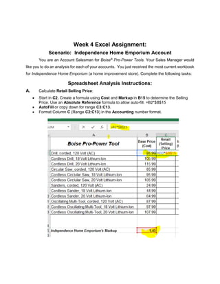
A. Calculate Retail Selling Price:
• Start in C2. Create a formula using Cost and Markup in B15 to determine the Selling
Price. Use an Absolute Reference formula to allow auto-fill. =B2*$B$15
• AutoFill or copy down for range C3:C13.
• Format Column C (Range C2:C13) in the Accounting number format.

2. B. Calculate the Inventory Value:
• Start in E2. Create a formula using Retail Selling Price and Inventory On-Hand to
determine the value of the product in the store. =C2*D2
• AutoFill or copy down for Column E (Range E3:E13). Resize column to fit all numbers.
• Format Column E (Range E2:E13) in the Currency number format.
C. Calculate the Sales:
• Start in G2. Create a formula that uses Retail Selling Price and Units Sold to
determine the dollar amount of product sold, year to date. =C2*F2
• AutoFill or copy down for Column G (Range G3:G13). Resize column to fit numbers.
• Format Column G (Range G2:G13) in the Accounting number format.
D. Calculate the Profit:
• Start in H2. Create a formula finds the difference between Retail Selling Price and
Cost, then multiply by Units Sold. =(C2-B2)*F2
• AutoFill or copy down for Column H (Range H3:H13).
• Format Column H (Range H2:H13) in the Accounting number format. Resize column to
fit numbers.
• In H14 use AutoSum to sum Column H (Range H2:H13).
• Add the text ‘Year to Date Profit Total’ in G14. Format G14 with Wrap Text and Center
both vertically and horizontally. Adjust Row and Column to fit. Bold both G14 and H14.

3. E. Apply Conditional Formatting to highlight products for re-order:
• Apply Conditional Formatting to Column D (Range D2:D13) calling attention to items
with an Inventory Less than 15 On-Hand. Use Green fill with Dark Green Text.
F. Apply Icon Sets under Conditional Formatting:
• Choose an Icon Set for the Range D2:D13 using Icon Sets from Conditional Formatting.

4. G. Boise®
Pro-Power Tools has added a new Hybrid Circular Saw; add the new product
to the analysis.
• Add a new row above “Sanders, corded, 120 Volt (AC).”
• Add the text “Circular Saw, Hybrid” to A8, 115.99 to B8, 24 to D8, 10 to F8.
• Calculate C8, E8 and G8 by copying down with AutoFill if it does not automatically
populate.
• Delete Row 6 (Cordless Circular Saw, 18 Volt Lithium-Ion) from the Worksheet.
H. Format as a Table with Headers:
• Highlight the Range A1:H14. Click the ‘Format as Table’ icon on the Home ribbon and
choose a table color theme. Make sure the ‘My Table has Headers’ box is checked,
then click ‘OK’. Resize all Rows and Columns to fit.

5. I. Show Profit (YTD) in a Column Chart:
• Select Column A (Range A1:A13) then hold the Control Key (CRTL) and Select
Column H (Range H1:H13). Do not click and release on A1 or H1 when highlighting.
Highlight A1:A13 and H1:H13 in one, fluid motion.
• Select Insert > choose Insert Column Chart > choose the first 2-D Column, Clustered
Column. Move the graph under the table.
J. Proof, compare and name your File:
• Proof your work and compare it to the sample below.
• Save your file using the naming convention:
APP101_your last name_week4_assignment.