1. Psychological Review
1988, Vol. 95, No. 3,371-38'
Copyright 1988 by the American Psychological Association, Inc.
0033-295X/88/S00.75
Contingent Weighting in Judgment and Choice
Amos Tversky Shmuel Sattath
Stanford University Hebrew University, Jerusalem, Israel
Paul Slovic
Decision Research, Eugene, Oregon
and Universityof Oregon
Preference can be inferred from direct choice between options or from a matching procedure in
which the decision maker adjusts one option to match another. Studies of preferences between two-
dimensional options (e.g., public policies, job applicants, benefit plans) show that the more promi-
nent dimension looms larger in choice than in matching. Thus, choice is more lexicographic than
matching. This finding is viewed as an instance of a generalprinciple of compatibility: The weighting
of inputs is enhanced by their compatibility with the output. To account for such effects, we develop
a hierarchyof models in which the trade-off between attributes is contingent on the nature of the
response. The simplest theory of this type, called the contingent weighting model, is applied to
the analysis of various compatibility effects, including the choice-matching discrepancy and the
preference-reversal phenomenon. These results raise both conceptual and practical questionscon-
cerning the nature, the meaning and the assessment of preference.
The relation of preference between acts or options is the key
element of decision theory that provides the basis for the mea-
surement of utility or value. In axiomatictreatments of decision
theory, the concept of preference appears as an abstract relation
that is given an empirical interpretation through specific meth-
ods of elicitation, such as choice and matching. In choice the
decision maker selects an option from an offered set of two or
more alternatives. In matchingthe decision maker is required to
set the value of some variable in order to achieve an equivalence
between options (e.g., what chance to win $750 is as attractive
as 1 chance in 10to win $2,500?).
The standard analysis of choice assumes procedure invari-
ance: Normatively equivalent procedures for assessing prefer-
ences should give rise to the same preference order. Indeed, the-
ories of measurement generally require the ordering of objects
to be independent of the particular method of assessment. In
classical physical measurement, it is commonly assumed that
each object possesses a well-defined quantity of the attribute
in question (e.g., length, mass) and that different measurement
procedures elicit the same ordering of objects with respect to
this attribute. Analogously, the classical theory of preference
assumes that each individual has a well-defined preference or-
der (or a utility function) and that different methods of elicita-
tion produce the same ordering of options. To determine the
heavier of two objects, for example, we can place them on the
two sides of a pan balance and observe which side goes down.
Alternatively, we can place each object separately on a sliding
scale and observe the position at which the sliding scale is bal-
anced. Similarly,to determine the preference order between op-
tions we can use either choice or matching. Note that the pan
This work was supported by Contract N00014-84-K-0615 from the
Office of Naval Research to Stanford University and by National Sci-
ence Foundation Grant 5ES-8712-145 to Decision Research.
The article has benefited from discussions with Greg Fischer, Dale
Griffin, Eric Johnson, Daniel Kahneman, and Lcnnart Sjtiberg.
balance is analogous to binary choice, whereas the sliding scale
resembles matching.
The assumption of procedure invariance is likely to hold
when people have well-articulated preferences and beliefs, as is
commonly assumed in the classical theory. If one likes opera
but not ballet, for example, this preference is likely to emerge
regardless of whether one compares the two directly or evalu-
ates them independently. Procedure invariance may hold even
in the absence of precomputed preferences, if people use a con-
sistent algorithm. We do not immediately know the value of
7(8 + 9), but we have an algorithm for computing it that yields
the same answer regardless of whether the addition is performed
before or after the multiplication. Similarly, procedure invari-
ance is likely to be satisfied if the value of each option is com-
puted by a well-defined criterion, such as expected utility.
Studies of decision and judgment, however, indicate that the
foregoing conditions for procedure invariance are not generally
true and that people often do not have well-defined values and
beliefs (e.g., Fischhoff, Slovic & Lichtenstein, 1980; March,
1978; Shafer & Tversky, 1985). In these situations, observed
preferences are not simply read off from some master list; they
are actually constructed in the elicitation process. Furthermore,
choice is contingent or context sensitive: It depends on the fram-
ing of the problem and on the method of elicitation (Payne,
1982; Slovic & Lichtenstein, 1983; Tversky & Kahneman,
1986). Different elicitation procedures highlight different as-
pects of options and suggest alternative heuristics, which may
give rise to inconsistent responses. An adequate account of
choice, therefore, requires a psychological analysis of the elicita-
tion process and its effect on the observed response.
What are the differences between choice and matching, and
how do they affect people's responses? Because our understand-
ing of the mental processes involved is limited, the analysis is
necessarily sketchy and incomplete. Nevertheless, there is rea-
son to expect that choice and matching may differ in a predict-
able manner. Consider the following example. Suppose Joan
371
2. 372 A. TVERSKY, S. SATTATH, AND P. SLOVIC
faces a choice between two job offers that vary in interest and
salary. Asa natural first step, Joan examineswhether one option
dominates the other (i.e., is superior in all respects). If not, she
may try to reframe the problem (e.g., by representing the op-
tions in terms of higher order attributes) to produce a dominant
alternative (Montgomery, 1983). If no dominance emerges, she
may examine next whether one option enjoys a decisive advan-
tage: that is, whether the advantage of one option far outweighs
the advantage of the other. If neither option has a decisive advan-
tage, the decision maker seeks a procedure for resolvingthe con-
flict. Because it is often unclear how to trade one attribute
against another, a common procedure for resolving conflict in
such situations is to select the option that is superior on the
more important attribute. This procedure, which is essentially
lexicographic, has two attractive features. First, it does not re-
quire the decision maker to assess the trade-off between the at-
tributes, thereby reducing mental effort and cognitive strain.
Second, it provides a compelling argument for choice that can
be used to justify the decision to oneself as well as to others.
Consider next the matching version of the problem. Suppose
Joan has to determine the salary at which the less interesting
job would be as attractive as the more interesting one. The qual-
itative procedure described earlier cannot be used to solve the
matching problem, which requires a quantitative assessment or
a matching of intervals. To perform this task adequately, the
decision maker should take into account both the size of the
intervals (defined relative to the natural range of variation of
the attributes in question)and the relative weightsof these attri-
butes. One method of matching first equates the size of the two
intervals, and then adjusts the constructed interval according
to the relative weight of the attribute. This approach is particu-
larly compelling when the attributes are expressed in the same
units (e.g., money, percent, test scores), but it may also be ap-
plied in other situations where it is easier to compare ranges
than to establish a rate of exchange. Because adjustments are
generally insufficient (Tversky & Kahneman, 1974) this proce-
dure is likely to induce a relatively flat or uniform weighting of
attributes.
The preceding discussion is not meant to provide a compre-
hensive account of choice or of matching. It merely suggests
different heuristics or computational schemes that are likely to
be used in the two tasks. If people tend to choose according
to the more important dimension, or if they match options by
adjusting unweighed intervals, then the two procedures are
likely to yield different results. In particular, choice is expected
to be more lexicographic than matching: That is, the more
prominent attribute will weigh more heavily in choice than in
matching. This is the prominence hypothesis investigated in the
following section.
The discrepancy between choice and matching was first ob-
served in a study by Slovic (1975) that was motivated by the
ancient philosophical puzzle of how to choose between equally
attractive alternatives. In this study the respondents first
matched different pairs of (two-dimensional) options and, in a
later session, chose between the matched options. Slovic found
that the subjects did not choose randomly but rather tended
to select the option that was superior on the more important
dimension. This observation supports the prominence hypoth-
esis, but the evidence is not conclusive for two reasons. First,
the participants always matched the options prior to the choice
hence the data could be explained by the hypothesis that the
more important dimension looms larger in the later trial. Sec-
ond, and more important, each participant chose between
matched options hence the results could reflect a common tie-
breaking procedure rather than a genuine reversal of prefer-
ences. After all, rationality does not entail a random breaking
of ties. A rational person may be indifferent between a cash
amount and a gamble but always pick the cash when forced to
take one of the two.
To overcome these difficulties we develop in the next section
a method for testing the prominence hypothesis that is based
entirely on interpersonal (between-subjects) comparisons, and
we apply this method to a variety of choice problems. In the
following two sections we present a conceptual and mathemati-
cal analysis of the elicitation process and apply it to several phe-
nomena of judgment and choice. The theoretical and practical
implications of the work are discussed in the final section.
Tests of the ProminenceHypothesis
Interpersonal Tests
We illustrate the experimental procedure and the logic of the
test of the prominence hypothesis in a problem involving a
choice between job candidates. The participants in the first set
of studies were young men and women (ages 20-30 years) who
were taking a series of aptitude tests at a vocational testing insti-
tute in Tel Aviv, Israel. The problems were presented in writing,
and the participants were tested in small groups. They all agreed
to take part in the study, knowing it had no bearing on their
test scores. Some of the results were replicated with Stanford
undergraduates.
Problem I (Production Engineer)
Imagine that, as an executive of a company, you have to select be-
tween two candidates for a position of a Production Engineer. The
candidates were interviewed by a committee who scored them on
two attributes (technical knowledge and human relations) on a
scale from 100 (superb) to 40 (very weak). Both attributes are im-
portant for the position in question, but technical knowledge is
more important than human relations. On the basis of the follow-
ing scores, which of the two candidates would you choose?
Candidate A"
Candidate Y
Technical
Knowledge
86
78
[AT-63]
Human
Relations
76
91 [35%]
The number of respondents (N) and the percentage who
chose each option are given in brackets on the right side of the
table. In this problem, about two thirds of the respondents se-
lected the candidate who has a higher score on the more impor-
tant attribute (technical knowledge).
Another group of respondents received the same data except
that one of the four scores was missing. They were asked "to
complete the missing score so that the two candidates would be
equally suitable for the job." Suppose, for example, that the
lower left value (78) were missing from the table. The respon-
dent's task would then be to generate a score for Candidate Y
in technical knowledge so as to match the two candidates. The
participants were reminded that "Yhas a higher score than X
in human relations, hence, to match the two candidates Y must
have a lower score than Xin technical knowledge."
3. CONTINGENT WEIGHTING 373
Assuming that higher scores are preferable to lower ones, it
is possible to infer the response to the choice task from the re-
sponse to the matching task. Suppose, for example, that one
produces a value of 80 in the matching task (when the missing
value is 78). This means that A"s score profile (86,76) isjudged
equivalent to the profile (80,91), which in turn dominates Y's
profile (78,91). Thus, a matching value of 80 indicates that X is
preferable to Y. More generally, a matching response above 78
implies a preference for X; a matching response below 78 im-
plies a preference for Y; and a matching response of 78 implies
indifference between X and Y.
Formally, let (Xi,X^ and (Yi,Y2) denote the values of options
X and y on Attributes 1and 2, respectively. Let Fhe the value
of YI for which the options are matched. We show that, under
the standard assumptions, A"is preferred to yif and only if V>
YI. Suppose V > Y,, then (XhXi) is equivalent to (V,Y2) by
matching, (V,Y^ is preferred to (Yt,Y2) by dominance, hence,
X is preferred to y by transitivity. The other cases are similar.
We use the subscript 1 to denote the primary, or the more
important dimension, and the subscript 2 to denote the second-
ary, or the less important dimension—whenever they are de-
fined. If neither option dominates the other, X denotes the op-
tion that is superior on the primary dimension and y denotes
the option that is superior on the secondary dimension. Thus,
Xt is better than Y, and y2 is better than X2.
Let C denote the percentage of respondents who chose X over
y, and let M denote the percentage of people whose matching
response favored X over Y. Thus, C and M measure the ten-
dency to decide according to the more important dimension in
the choice and in the matching tasks, respectively. Assuming
random allocation of subjects, procedure invariance implies
C — M, whereas the prominence hypothesis implies C > M. As
was shown earlier, the two contrasting predictions can be tested
by using aggregate between-subjects data.
To estimate M, we presented four different groups of about
60 respondents each with the data of Problem 1, each with a
different missing value, and we asked them to match the two
candidates. The following table presents the values of M derived
from the matching data for each of the four missing values,
which are given in parentheses.
1. Technical Knowledge 2. HumanRelations
Candidate Jf 32% (86) 33% (76)
Candidate Y 44%(78) 26%(91)
There were no significant differences among the four matching
groups, although M was greater when the missing valuewas low
rather than high (ML = 39 > 29 = MH) and when the missing
value referred to the primary rather than to the secondary attri-
bute (Mi = 38 > 30 = Af2). Overall, the matching data yielded
M = 34% ascompared with C - 65% obtained from choice (p <
.01). This result supports the hypothesis that the more impor-
tant attribute (e.g., technical knowledge) looms larger in choice
than in matching.
In Problem 1, it is reasonable to assume—as stated—that for
a production engineer, technical knowledge is more important
than human relations. Problem 2 had the same structure as
Problem 1, except that the primary and secondary attributes
were manipulated. Problem 2 dealt with the choice between
candidates for the position of an advertising agent. The candi-
dates were characterized by their scores on two dimensions: cre-
ativity and competence. One half of the participants were told
that "for the position in question, creativity is more important
than competence," whereas the other half of the participants
were told the opposite. As in Problem 1, most participants
(65%, N = 60) chose according to the more important attribute
(whether it was creativity or competence) but only 38% (N =
276) of the matching responses favored X over Y.Again, M was
higher for the primary than for the secondary attribute, but all
four values of M were smaller than C. The next two problems
involve policy choices concerning safety and the environment.
Problem 3 (Traffic Accidents)
About 600 people are killed each year in Israel in traffic accidents.
The ministry of transportation investigates various programs to
reduce the number of casualties.Consider the following two pro-
grams, described in terms of yearly costs (in millions of dollars)
and the number of casualties per year that is expected following the
implementation of each program.
Program X
Program Y
Expected number
of casualties
500
570
Cost
$55M
$12M
[JV =96]
[67%]
[33%]
Which program do you favor?
The data on the right side of the table indicate that two thirds
of the respondents chose Program X, which saves more lives at
a higher cost per life saved. Twoother groups matched the cost
of either Program X or Program y so as to make the two pro-
grams equally attractive. The overwhelming majority of match-
ing responses in both groups (96%, N = 146) favored the more
economical Program y that saves fewer lives. Problem 3 yields
a dramatic violation of invariance: C = 68%but M = 4%. This
pattern follows from the prominence hypothesis, assuming the
number of casualties is more important than cost. There was
no difference between the groups that matched the high ($55M)
or the low ($ 12M) values.
A similar pattern of responses was observed in Problem 4,
which involves an environmental issue. The participants were
asked to compare two programs for the control of a polluted
beach:
Program X: A comprehensive program for a complete clean-up of
the beach at a yearly cost of $750,000 to the taxpayers.
Program Y:A limited program for a partial clean-up of the beach
(that will not make it suitable for swimming) at a yearly cost of
$250,000 to the taxpayers.
Assuming the control of pollution is the primary dimension
and the cost is secondary, we expect that the comprehensive
program will be more popular in choice than in matching.This
prediction was confirmed: C = 48% (N = 104) and M = 12%
(N = 170). The matching data were obtained from two groups
of respondents who assessed the cost of each program so as to
match the other. As in Problem 3, these groups gave rise to prac-
tically identical values of M.
Because the choice and the matching procedures are strategi-
cally equivalent, the rational theory of choice implies C = M.
The two procedures, however, are not informationally equiva-
lent because the missing value in the matching task is available
in the choice task. Tocreate an informationally equivalent task
we modified the matchingtask by asking respondents, prior to
the assessment of the missing value, (a) to consider the value
4. 374 A. TVERSKY, S. SATTATH, AND P. SLOVIC
Table 1
Percentages of Responses Favoring the Primary Dimension Under Different Elicitation Procedures
Dimensions
Problem:
1. Engineer
N
2. Agent
N
3. Accidents
N
4. Pollution
N
5. Benefits
N
6. Coupons
N
Unweighted mean
Primary
Technical knowledge
Competence
Casualties
Health
1 year
Books
Secondary
Human relations
Creativity
Cost
Cost
4 years
Travel
Choice
(C)
65
63
65
60
68
105
48
104
59
56
66
58
62
Information
control
C*
57
156
52
155
50
96
32
103
48
M*
47
151
41
152
18
82
12
94
30
Matching
(M)
34
267
38
276
4
146
12
170
46
46
11
193
24
»
.82
.72
.19
.45
.86
.57
C = percentage of respondents who chose X over Y;M — percentage of respondents whose matching responses favored X over Y C* = percentage
of responses to Question a that lead to the choice ofX; M' =percentage of matching responses to Question b that favor option X.
used in the choice problem and indicate first whether it is too
high or too low, and (b) to write down the value that they con-
sider appropriate. In Problem 3, for example, the modified pro-
cedure read as follows:
Program X
Program Y
Expected number
of casualties
500
570
Cost
?
$I2M
You are asked to determine the cost of Program A"that would make
it equivalent to Program Y,(a) Is the value of $55M too high or too
low? (b) What is the value you consider appropriate?
The modified matchingprocedure is equivalentto choice not
only strategically but also informationally. Let C* be the pro-
portion of responses to question (a) that lead to the choice of
X (e.g., "too low" in the preceding example). Let M" be the
proportion of (matching) responses to question (b) that favor
option X (e.g., a value that exceeds $55M in the preceding ex-
ample). Thus, we may view C*as choice in a matching context
and M* as matching in a choice context. The values of C* and
M' for Problems 1 -4 are presented in Table 1, which yields the
ordering C > C' > M' > M. The finding C> C' shows that
merely framing the question in a matching context reduces the
relative weight of the primary dimension. Conversely, M" > M
indicates that placing the matching task after a choice-like task
increases the relative weight of the primary dimension. Finally,
C">M* implies a within-subject and within-problem violation
of invariance in which the response to Question a favors X and
the response to Question b favors Y. This pattern of responses
indicates a failure, on the part of some subjects, to appreciate
the logical connection between Questions a and b. It is notewor-
thy, however, that 86% of these inconsistencies follow the pat-
tern implied by the prominence hypothesis.
In the previous problems, the primary and the secondary at-
tributes were controlled by the instructions, as in Problems 1
and 2, or by the intrinsic value of the attributes, as in Problems
3 and 4. (People generallyagree that saving lives and eliminating
pollution are more important goals than cutting public expen-
ditures.)The next two problems involvedbenefit plans in which
the primary and the secondary dimensions were determined by
economic considerations.
Problem 5 (Benefit Plans)
Imagine that, as a part of a profit-sharing program, your employer
offers you a choice between the following plans. Each plan offers
two payments, in one year and in four years.
Plan*
PlanK
Payment in
I year
$2,000
$1,000
Payment in
4 years
$2,000
$4,000
(N =361
[59%]
[41%]
Which plan do you prefer?
Because people surely prefer to receive a payment sooner
rather than later, weassume that the earlier payment (in 1year)
acts as the primary attribute, and the later payment (in 4 years)
acts as the secondary attribute. The results support the hypoth-
esis: C = 59% (N = 56) whereas M = 46% (TV = 46).
Problem 6 resembled Problem 5 except that the employee
was offered a choice between two bonus plans consisting of a
different combination of coupons for books and for travel. Be-
cause the former could be used in a large chain of bookstores,
whereas the latter were limited to organized tours with a partic-
ular travel agency, we assumed that the book coupons would
serve as the primary dimension. Under this interpretation, the
prominence effect emerged again: C = 66%(N = 58) and M =
11% (N — 193). As in previous problems, M was greater when
the missing value was lowrather than high (ML = 17 > 3 = MH)
and when the missing value referred to the primary rather than
the secondary attribute (Mi = 19 > 4 = A/2). All values of M,
however, were substantially smaller than C.
5. CONTINGENT WEIGHTING 375
Table 2
Percentages of Respondents (N = 101) Who Chose Between-Matched Alternatives (M = 50%)
According to the Primary Dimension (After Slavic, 1975)
Dimensions
Alternatives Primary Secondary
C = percentage of respondents who chose X over Y.
Choice criterion
1. Baseball players
2. College applicants
3. Gifts
4. Typists
5. Athletes
6. Routes to work
7. Auto tires
8. TV commercials
9. Readers
10. Baseball teams
Unweighted
mean
Batting average
Motivation
Cash
Accuracy
Chin-ups
Time
Quality
Number
Comprehension
% of games won against first place team
Home runs
English
Coupons
Speed
Push-ups
Distance
Price
Time
Speed
% of games won agains last place team
Value to team
Potentialsuccess
Attractiveness
Typing ability
Fitness
Attractiveness
Attractiveness
Annoyance
Readingability
Standing
62
69
85
84
68
75
67
83
79
86
76
Intrapersonal Tests
Slovic's (1975) original demonstration of the choice-match-
ing discrepancy wasbased entirely on an intrapersonal analysis.
In his design, the participants first matched the relevant option
and then selected between the matched options at a later date.
They were also asked afterward to indicate the more important
attribute in each case. The main results are summarized in Ta-
ble 2, which presents for each choice problem the options, the
primary and the secondary attributes, and the resultingvalues
of C. In every case, the value of M is 50%by construction.
The results indicate that, in all problems, the majority of par-
ticipants broke the tie betweenthe matched options in the direc-
tion of the more important dimension as implied by the promi-
nence hypothesis. This conclusion held regardless of whether
the estimated missing value belonged to the primary or the sec-
ondary dimension, or whether it was the high value or the low
value on the dimension. Note that the results of Table 2 alone
could be explained by a shift in weight following the matching
procedure (because the matching always preceded the choice)
or by the application of a common tie-breaking procedure (be-
cause for each participant the two options were matched). These
explanations, however, do not apply to the interpersonal data of
Table 1.
On the other hand, Table 2 demonstrates the prominence
effect within the data of each subject. The value of C was only
slightly higher (unweighted mean: 78) when computed relative
to each subject's ordering of the importance of the dimensions
(as was done in the original analysis), presumably because of
the general agreement among the respondents about which di-
mension was primary.
Theoretical Analysis
The data described in the previous section show that the pri-
mary dimension looms larger in choice than in matching. This
effect gives rise to a marked discrepancy between choice and
matching, which violates the principleof procedure invariance
assumed in the rational theory of choice. The prominence effect
raises three general questions. First, what are the psychological
mechanisms that underlie the choice-matching discrepancy and
other failures of procedure invariance? Second, what changes
in the traditional theory are required in order to accommodate
these effects? Third, what are the implications of the present
results to the analysis of choice in general, and the elicitation of
preference in particular? The remainder of this article is de-
voted to these questions.
The Compatibility Principle
One possible explanation of the prominence effect, intro-
duced earlier in this article, is the tendency to select the option
that is superior on the primary dimension, in situations where
the other option does not have a decisive advantage on the sec-
ondary dimension. This procedure is easy to apply and justify
because it resolvesconflict on the basis of qualitative arguments
(i.e., the prominence orderingof the dimensions)without estab-
lishing a rate of exchange. The matching task, on the other
hand, cannot be resolved in the same manner. The decision
maker must resort to quantitative comparisons to determine
what interval on one dimension matches a given interval on the
second dimension. This requires the setting of a common met-
ric in which the attributes are likely to be weighted more
equally, particularly when it is natural to match their ranges or
to compute cost per unit (e.g., the amount of money spent to
save a single life).
It is instructive to distinguish between qualitativeand quanti-
tative arguments for choice. Qualitative, or ordinal, arguments
are based on the ordering of the levels within each dimension,
or on the prominence ordering of the dimensions. Quantitative,
or cardinal, arguments are based on the comparison of value
differences along the primary and the secondary dimensions.
Thus, dominanceand a lexicographicordering are purelyquali-
tative decision rules, whereas most other models of multiattri-
bute choice make essential use of quantitative considerations.
The prominence effect indicates that qualitative considerations
loom largerin the ordinal procedure of choice than in the cardi-
6. 376 A. TVERSK.Y, S. SATTATH, AND P. SLOVIC
nal procedure of matching, or equivalently, that quantitative
considerations loom larger in matching than in choice. The
prominence hypothesis, therefore, may be construed as an ex-
ample of a more general principle of compatibility.
The choice-matching discrepancy, like other violations of
procedure invariance, indicates that the weighting of the attri-
butes is influenced by the method of elicitation. Alternative
procedures appear to highlight different aspects of the options
and thereby induce different weights. To interpret and predict
such effects, we seek explanatory principles that relate task
characteristics to the weighting of attributes and the evaluation
of options. One such explanation is the compatibility principle.
According to this principle, the weight of any input component
is enhanced by its compatibility with the output. The rationale
for this principle is that the characteristics of the task and the
response scale prime the most compatible features of the stimu-
lus. For example, the pricing of gambles is likely to emphasize
payoffs more than probability because both the response and
the payoffs are expressed in dollars. Furthermore,noncompati-
bility (in content, scale, or display) between the input and the
output requires additional mental transformations, which in-
crease effort and error, and reduce confidence and impact (Fitts
& Seeger, 1953; Wickens, 1984). We shall next illustrate the
compatibility principle in studies of prediction and similarity
and then developa formal theory that encompasses a variety of
compatibility effects, including the choice-matching discrep-
ancy and the preference reversal phenomenon.
A simple demonstration of scale compatibility was obtained
in a study by Slovic, Griffin, and, Tversky (1988). The subjects
(N = 234) were asked to predict the judgments of an admission
committee of a small, selective college. For each of 10 applicants
the subjects received two items of information: a rank on the
verbal section of the Scholastic Aptitude Test (SAT) and the
presence or absence of strong extracurricular activities. The
subjects were told that the admission committee ranks all 500
applicants and accepts about the top fourth. Half of the subjects
predicted the rank assigned to each applicant, whereas the other
half predicted whether each applicant was accepted or rejected.
The compatibility principle implies that the numerical data
(i.e., SAT rank) will loom larger in the numerical prediction
task, whereas the categorical data (i.e., the presence or absence
of extracurricular activities) will loom larger in the categorical
prediction of acceptance or rejection. The results confirmed the
hypothesis. For each pair of applicants, in which neither one
dominates the other, the percentage of responses that favored
the applicant with the higher SAT was recorded. Summing
across all pairs, this value was 61.4% in the numerical predic-
tion task and 44.6% in the categorical prediction task. The
difference between the groups is highly significant. Evidently,
the numerical data had more impact in the numerical task,
whereas the categorical data had more impact in the categorical
task. This result demonstrates the compatibility principle and
reinforces the proposed interpretation of the choice-matching
discrepancy in which the relative weight of qualitative argu-
ments is larger in the qualitative method of choice than in the
quantitative matching procedure.
In the previous example, compatibility was induced by the
formal correspondence between the scales of the dependent and
the independent variables. Compatibility effects can also be in-
duced by semantic correspondence, as illustrated in the follow-
ing example, taken from the study of similarity. In general, the
similarity of objects (e.g., faces, people, letters) increases with
the salience of the features they share and decreases with the
salience of the features that distinguish between them. More
specifically, the contrast model (Tversky, 1977) represents the
similarity of objects as a linear combination of the measures of
their common and their distinctive features. Thus, the similar-
ity of a and b is monotonically related to
where ,4 Pi .ff is the set of features shared by a and b, and A A£ =
(A - B)U(B - A)isthesetof features that belongs to one object
and not to the other. The scales/and g are the measures of the
respective feature sets.
The compatibility hypothesis suggests that common features
loom larger in judgments of similarity than in judgments of dis-
similarity, whereasdistinctive featuresloom larger in judgments
of dissimilarity than in judgments of similarity. As a conse-
quence, the two judgments are not mirror images. A pair of
objects with many common and many distinctive features
could bejudged as more similar, as well as more dissimilar, than
another pair of objects with fewer common and fewer distinctive
features. Tversky and Gati (1978) observed this pattern in the
comparison of pairs of well-known countries with pairs of
countries that were less well-knownto the respondents. For ex-
ample, most subjects in the similarity condition selected East
Germany and West Germany as more similar to each other than
Sri Lanka and Nepal, whereas most subjects in the dissimilarity
condition selected East Germany and West Germany as more
different from each other than Sri Lanka and Nepal. These ob-
servations were explained by the contrast model with the added
assumption that the relative weight of the common features is
greater in similarity than in disimilarity judgments (Tversky,
1977).
Contingent Trade-Off Models
To accommodate the compatibility effects observed in stud-
ies of preference, prediction and judgment, we need models in
which the trade-offs among inputs depend on the nature of the
output. In the present section wedevelop a hierarchy of models
of this type, called contingent trade-off models. For simplicity,
we investigate the two-dimensional case and follow the choice-
matching terminology. Extensions and applications are dis-
cussed later. It is convenient to use A = {a,b,c, . . . } and Z =
{z.y.x, . . . } to denote the primary and the secondary attri-
butes, respectively, wheneverthey are properly defined. The ob-
ject setS is given by the product setA X Z, with typical elements
az, by, and so on. Let ac be the preference relation obtained
by choice, and let sm be the preference relation derived from
matching.
As in the standard analysis of indifference curves (e.g.,
Varian, 1984, chap. 3), we assume that each &u i = c,m, is a
weak order, that is, reflexive, connected, and transitive. We also
assume that the levels of each attribute are consistently ordered,
independent of the (fixed) level of the other attribute. That is,
azi^ibz iff ay^by and az>jay iff bz^iby, i = c,m.
Under these assumptions, in conjunction with the appropriate
7. CONTINGENT WEIGHTING 377
matching
choice
Primary Attribute
Figure 1. A dual indifference map induced by the
general model (Equations 1and 2).
structural conditions (see,e.g., Krantz, Luce, Suppes & Tver-
sky, 1971, chap. 7), there exist functions F, GI, and Ut, defined
on A, Z, and Re X Re, respectively, such that
az^byiSfUt
[Fi(a),Gi(z)] a. U)
where 14 i = c,m is monotonically increasing in each of its ar-
guments.
Equation 1 imposes no constraints on the relation between
choice and matching. Although our data show that the two or-
ders do not generally coincide, it seems reasonable to suppose
that they do coincide in uniditnensional comparisons. Thus, we
assume
az^joz iff az^.m
bz and az^ay iff az^m
ay.
It is easy to see that this condition is both necessary and suffi-
cient for the monotonicity of the respective scales. That is,
FJb) 2= Fc
(a) iffFm
(b) ;> Fm
(a) and (2)
G,(z) a Gc(y) iffGm(z) & Gm(y).
Equations 1 and 2 define the general contingent trade-off
model that is assumed throughout. The other models discussed
in this section are obtained by imposing further restrictions on
the relation between choice and matching. The general model
corresponds to a dual indifference map, that is, two families of
indifference curves, one induced by choice and one induced by
matching. A graphical illustration of a dual map is presented in
Figure 1.
We next consider a more restrictive model that constrains the
relation between the rates of substitution of the two attributes
obtained by the two elicitation procedures. Suppose the in-
difference curves are differentiable, and let RS denote the rate
of substitution between the two attributes (A and Z) according
to procedure ;' = c,m. Thus, RSi = F'-JG,, where F-, and G,
respectively, are the partial derivatives of U> with respect to Ft
and G{. Hence, RSi(az) is the negative of the slope of the in-
difference curve at the point az. Note that RS is a meaningful
quantity even though F,,Gi and U{
are only ordinal scales.
A contingent trade-off model is proportional if the ratio of
RSC
to RSm
is the same at each point. That is,
RSc(az)/RSm(az) = constant. (3)
Recall that in the standard economic model, the foregoing
ratio equals 1 . The proportional model assumes that this ratio
is a constant, but not necessarily one. The indifference maps
induced by choice and by matching, therefore, can be mapped
into each other by multiplying the RS value at every point by
the same constant.
Both the general and the proportional model impose fewcon-
straints on the utility functions Ui. In many situations, prefer-
ences between multiattribute options can be represented addi-
tively. That is, there exist functions Fi and G defined on A and
Z, respectively, such that
az^by KF{
(a) + GJz) ;> F{
(b) + G-,(y), i = c,m, (4)
where F-, and Gj are interval scales with a common unit. The
existence of such an additive representation is tantamount to
the existence of a monotone transformation of the axes that
maps all indifference curves into parallel straight lines.
Assuming the contingent trade-off model, with the appropri-
ate structural conditions, the following cancellation condition
is both necessary and sufficient for additivity (Equation 4), see
Krantz et al. (1 97 1 , chap. 6):
ajfe-ibx and bz^.cy imply az^cx, i = c,m.
If both proportionality and additivity are assumed, we obtain
a particularly simple form, called the contingent weighting
model, in which the utility scales Fc,Fm and Gc,Gm are linearly
related. In other words, there is a monotone transformation of
the axes that simultaneously linearizes both sets of indifference
curves. Thus, if both Equations 3 and 4 hold, there exist func-
tions F and G defined on A and Z, respectively, and constants
«ift, i = c,m, such that
az^iby iff of (a) + №(z) ;> af(b) + faG(y) (5)
iffFfa) + 6(G(z) ^ F(b) + 9&(y),
where 0i = ft/a*. In this model, therefore, the indifference maps
induced by choice and by matching are represented as two sets
of parallel straight lines that differ only in slope -ft, i = c,m(see
Figure 2). We are primarily interested in the ratio 9 = 0c/flm of
these slopes.
Because the rate of substitution in the additive model is con-
stant, it is possible to test proportionality (Equation 3) without
assessing local RSi. In particular, the contingent weighting
model (Equation 5) implies the following interlocking condi-
tion;
ax^Jbw, az imply
and the same holds when the attributes (A and Z) and the orders
(2:c and fcm) are interchanged. Figure 3 presents a graphic illus-
tration of this condition. The interlocking condition is closely
related to triple cancellation, or the Reidemeister condition (see
8. 378 A. TVERSKY, S. SATTATH, AND P. SLOVIC
Primary Attribute
Figure 2. A dual indifference map induced by
the additive model (Equation 4).
Krantz et al., 1971,6.2.1), tested by Coombs, Bezembinder,and
Goode (1967). The major difference between the assumptions
is that the present interlocking condition involves two orders
rather than one. This condition says, in effect, that the intradi-
mensional ordering of -4-intervals or Z-intervals is independent
of the method of elicitation. This can be seen most clearly by
deriving the interlocking condition from the contingentweight-
ing model. From the hypotheses of the condition, in conjunc-
tion with the model, we obtain
Figure 4. A hierarchy of contingent preference models.
(Implications are denoted by arrows.)
F(a) + 6,,G(x) > F(b) + ffcG(w) or
F(d) + 6cG(w) > F(c) + 6cG(x) or
F(d)-F(c)*ec[G(x)-G(w)]
F(b) + 9mG(y) ^ F(a) + BmG(z) or
F(b) - F(a) ^ 8m[G(z) - G(y)].
The right-hand inequalitiesyield
F(d) - F(c) & 9m(G(z) - G(y)] or
F(d) + 6mG(y) ^ F(c) + 9mG(z),
hence dy^mcz as required.
The interlocking condition is not only necessary but also
sufficient, because it implies that the inequalities
Fi(d) - Fife) ^ Fi(b) - f(a) and
Gi(z) - Gi(y) > Gi(x) - GM
are independent of i = c,m, that is, the two procedures yield
the same ordering of intradimcnsional intervals. But becauseFc
and Fm (as well as Gc and Gm)are interval scales, they must be
linearly related. Thus, there exist functions F and G and con-
stants aj, ft such that
Figure 3. A graphic illustration of the interlocking con-
dition where arrows denote preferences.
Thus, wehave established the following result.
Theorem: Assuming additivity (Equation 4), the contingent
weighting model (Equation 5) holds iff the interlocking condition
is satisfied.
Perhaps the simplest, and most restrictive, instance of Equa-
tion 5 is the case where A and Z are sets of real numbers and
both Fand Gare linear. In this case, the model reduces to
az^-tby iff aa + ftz a aj) + fty (6)
iffcz + 0jZ & b + 6y, 0j = /3r/«i, i = c,m.
The hierarchy of contingent trade-off models is presented in
Figure 4, whereimplications are denoted byarrows.
In the following section we apply the contingent weighting
model to several sets of data and estimate the relative weights
9. CONTINGENT WEIGHTING 379
of the two attributes under different elicitation procedures. Nat-
urally, all the models of Figure4 are consistent with the compat-
ibility hypothesis. We use the linear model (Equation 6) because
it is highly parsimonious and reduces the estimation to a single
parameter 8 - 6J9m. If linearity of scales or additivity of attri-
butes is seriously violated in the data, higher models in the hier-
archy should be used. The contingent weighting model can be
readily extended to deal with more than two attributes and
methods of elicitation.
The same formal model can be applied when the different
preference orders Sj are generated by different individuals
rather than by different procedures. Indeed, the interlocking
condition is both necessary and sufficient for representing the
(additive) preference orders of different individuals as varia-
tions in the weighting of attributes. (This notion underlies the
INDSCAL approach to multidimensional scaling, Carroll, 1972).
The two representations can be naturally combined to accom-
modate both individual differences and procedural variations.
The following analyses focus on the latter problem.
Applications
The Choice-Matching Discrepancy
We first compute 9 = 6cjf>m from the choice and matching
data, summarized in Table 1. Let C(az,by) be the percentage
of respondents who chose az over by, and let M(az,by) be the
percentage of respondents whose matching response favored az
over by. Consider the respondents who matched the options by
adjusting the second component of the second option. Because
different respondents produced different values of the missing
component (y), we can view M(az,b.) as a (decreasing) function
of the missing component. Let y be the value of the second attri-
bute for which M(az,by) - C(az,by).
If the choice and the matching agree, j> should be equal to y,
whereas the prominence hypothesis implies that y lies between
y and z (i.e., |z - y > z - y). Toestimate 6 from these data,
we introduce an additional assumption, in the spirit of probabi-
listic conjoint measurement (Falmagne, 1985,chap. 11), which
relates the linear model (6) to the observed percentage of re-
sponses.
(a
M(az,by) = C(az,by) iff
) -fb + emy) = (a + 6cz) -fb + 9cy) iff (7)
0mfz ~'y) = 8c(z - y).
Under this assumption wecan compute
and the same analysis applies to the other three components
(i.e., it, b, and z).
We applied this method to the aggregate data from Problems
1 to 6. The averagevalues of 0, across subjects and components,
are displayedin Table 1 for each of the six problems. The values
of B = 9J8m are all less than unity, as implied by the prominence
hypothesis. Note that 6 provides an alternative index of the
choice-matching discrepancy that is based on Equations 6 and
7—unlike the difference between Cand Mthat does not presup-
pose any measurement structure.
Prediction of Performance
We next use the contingent weighting model to analyze the
effect of scale compatibility observed in a study of the predic-
tion of students' performance, conducted by Slovic et al. ( 1 988).
The subjects (N = 234) in this study were asked to predict the
performance of 10 students in a course (e.g., History) on the
basis of their performance in two other courses (e.g., Philosophy
and English). For each of the 10 students, the subjects received
a grade in one course (from A to D), and a class rank (from 1
to 100) in the other course. One half of the respondents were
asked to predict a grade, and the other half were asked to predict
class rank. The courses were counterbalanced across respon-
dents. The compatibilityprinciple implies that a given predic-
tor (e.g., grade in Philosophy) will be given more weight when
the predicted variable is expressed on the same scale (e.g., grade
in History) than when it is expressed on a different scale (e.g.,
class rank in History). The relative weight of grades to ranks,
therefore, will be higher in the group that predicts grades than
in the group that predicts ranks.
Let (rj, gj) be a student profile with rank i in the first course
and grade,; in the second. Let r-,j and g% denote, respectively, the
predicted rank and grade of that student. The ranks range from
1 to 100, and the grades were scored as A+ = 10, A = 9, . . . ,
D = 1 .Under the linear model (Equation 6), we have
rij = a,r, + frgj and g$ = a^ + 0^
By regressing the 10 predictions of each respondent against the
predictors, r and g, we obtained for each subject in the rank
condition an estimate of 0r = fi,/a,, and for each subject in the
grade condition an estimate of 0g = j3,/ae. These values reflect
the relative weight of grades to ranksin the two prediction tasks.
As implied by the compatibility hypothesis,the values of 0, were
significantly higher than the values of 0,, p < .001 by a Mann-
Whitney test.
Figure 5 represents each of the 10 students as a point in the
rank Xgrade plane. The slopes of the two lines, 9r and 0g, corre-
spond to the relative weights of grade to rank estimated from
the average predictions of ranks and grades, respectively. The
multiple correlation between the inputs (r, gj) and the average
predicted scores was .99 for ranks and .98 for grades, indicating
that the linear model provides a good description of the aggre-
gate data. Recall that in the contingent weighting model, the
predicted scores are given by the perpendicular projections of
the points onto the respective lines, indicated by notches. The
two lines, then, are orthogonal to the equal-value sets denned
by the two tasks. The figure shows that grades and ranks were
roughly equally weightedin the prediction of grades (0, = 1 .06),
but grades were given much less weight than ranks in the predic-
tion of ranks (6, = .58). As a consequence, the two groupsgener-
ated different ordering of the students. For example, the pre-
dicted rank of Student 9 was higher than that of Student 8, but
the order of the predicted grades was reversed. Note that the
numbered points in Figure 5 represent the design, not the data.
The discrepancy between the two orderings is determined
jointly by the angle between the lines that is estimated from
subjects' predictions, and by the correlation between the two
dimensions that is determined by the design.
These data suggest a more detailed account based on a pro-
cess of anchoringand adjustment (Slovic & Lichtenstein, 1971;
10. 380 A. TVERSKY, S. SATTATH, AND P. SLOVIC
A-f
A-
^. B+
B-
c-
100 90 80 70 0 50 40
Rank (n)
30 20 10
Figure 5. Contingent weighting representation of predicted ranks and grades. (Thedots characterize the
input information for each of the 10 students. The slopes of the two lines correspond to the relative weight
of grades to ranks in the two prediction tasks.)
Tversky & Kahneman, 1974). According to this heuristic, the
subject uses the score on the compatible attribute (either rank
or grade) as an anchor, and adjusts it upward or downward on
the basis of the other score. Because adjustments are generally
insufficient, the compatible attribute is overweighted. Although
the use of anchoring and adjustment probably contribute to the
phenomenon in question, Slovic et al. (1988) found a significant
compatibility effect even when the subject only predicted which
of the two students would obtain a higher grade (or rank), with-
out making any numerical prediction that calls for anchoring
and adjustment.
Preference Reversals
The contingent weighting model (Equation 5) and the com-
patibility principle can also be used to explain the well-known
preference reversals discovered by Lichtenstein and Slovic
(1971; see also Slovic and Lichtenstein, 1968, 1983). These in-
vestigators compared two types of bets with comparable ex-
pected values—an H bet that offers a high probability of win-
ning a relatively small amount of money (e.g., 32/36 chance to
win $4) and an L bet that offers a low probability of winning a
moderate amount of money (e.g., 9/36 chance to win $40). The
results show that people generally choose the // bet over the L
bet (i.e., H >c L) but assign a higher cash equivalent to the L
bet than to the // bet (i.e., CL > CH, where CL and CH are the
amounts of money that are as desirable as L and H respec-
tively). This pattern of preferences, which is inconsistent with
the theory of rational choice, has been observed in numerous
experiments, including a study conducted on the floor of a Las
Vegas casino (Lichtenstein & Slovic, 1973), and it persists even
in the presence of monetary incentives designed to promote
consistent responses (Grether & Plott, 1979).
Although the basic phenomenon has been replicated in many
studies, the determinants of preference reversals and their
causes have remained elusive heretofore. It is easy to show that
the reversal of preferences implies either intransitive choices or
a choice-pricing discrepancy (i.e., a failure of invariance), or
11. CONTINGENT WEIGHTING 381
both. In order to understand this phenomenon, it is necessary
to assess the relative contribution of these factors because they
imply different explanations. To accomplish this goal, however,
one must extend the traditional design and include, in addition
to the bets H and L, a cash amount X that is compared with
both. If procedure invariance holds and preferencereversals are
due to intransitive choices, then weshould obtain the cycle L >c
X>CH>CL. If, on the other hand, transitivity holds and prefer-
ence reversals are due to an inconsistency between choice and
pricing, then we should obtain either X >c L and CL > X, or
H>CX and X > CH. The first pattern indicates that L is over-
priced relative to choice, and the second pattern indicates that
H is underpriced relative to choice. Recall that H>CX refers to
the choice between the bet H and the sure thing X, while X >
CH refers to the ordering of cash amounts.
Following this analysis, Tversky, Slovic, and Kahneman
(1988) conducted an extensive study of preference reversals, us-
ing 18 triples (H,L,X) that cover a wide range of probabilities
and payoffs. A detailed analysis of response patterns showed
that, by far, the most important determinant of preference re-
versals is the overpricing of/,. Intransitive choices and the un-
derpricing of H play a relatively minor role, each accounting
for less than 10% of the total number of reversals. Evidently,
preference reversals represent a choice-pricing discrepancy in-
duced by the compatibility principle: Because pricing is ex-
pressed in monetary units, the payoffs loom larger in pricing
than in choice.
We next apply the contingent weighting model to a study re-
ported by Tversky et al. (1988) in which 179 participants (a)
chose between 6 pairs consisting of an H bet and an L bet, (b)
rated the attractiveness of all 12 bets, and (c) determined the
cash equivalent of each bet. In order to provide monetary incen-
tives and assure the strategic equivalence of the three methods,
the participants were informed that a pair of bets would be se-
lected at random, and that they would play the member of the
pair that they had chosen, or the bet that they had priced or
rated higher. The present discussion focuses on the relation be-
tween pricing and rating, which can be readily analyzed using
multiple regression. In general, rating resembles choice in fa-
voring the H bets, in contrast to pricing that favors the L bets.
Note that in rating and pricing each gamble is evaluated sepa-
rately, whereas choice (and matching) involvea comparison be-
tween gambles. Because the discrepancy between rating and
pricing is even more pronounced than that between choice and
pricing, the reversal of preferences cannot be explained by the
fact that choice is comparative whereas pricing is singular. For
further discussions of the relation between rating, choice, and
pricing, see Goldstein and Einhom (1987), and Schkade and
Johnson (1987).
We assume that the value of a simple prospect (q,y) is approx-
imated by a multiplicative function of the probability g and the
payoff y. Thus, the logarithms of the pricing and the rating can
be expressed by
0i log y + log q, i = r,p, (8)
where 0, and ffp denote the relative weight of the payoff in the
rating and in the pricing tasks, respectively. Note that this
model implies a power utility function with an exponent ft. The
average transformed rating and pricing responses for each of
the 12 bets were regressed, separately, against log q and log y.
The multiple correlations were .96 and .98 for the ratings and
the pricing, respectively, indicating that the relation between
rating and pricing can be captured, at least in the aggregate
data, by a very simple model with a single parameter.
Figure 6 represents each of the 12 bets as a (numbered) point
in the plane whose coordinates are probability and money, plot-
ted on a logarithmic scale. The rating and pricing lines in the
figure are perpendicular to the respective sets of linear indiffer-
ence curves (see Figure 2). Hence, the projections of each bet
on the two lines (denoted by notches) correspond to their values
derived from rating and pricing, respectively. The anglebetween
these lines equals the (smaller) angle between the intersecting
families of indifference curves. Figure 6 reveals a dramatic
difference between the slopes: 8, = 2.7, flp =.75, hence 6 = Of/
6, = .28. Indeed, these data give rise to a negative correlation
(r = —.30) between the rating and the pricing, yielding numer-
ous reversals of the ordering of the projections on the two lines.
For example, the most extreme L bet (No. 8) has the lowest
rating and the highest cash equivalent in the set.
The preceding analysis shows that the compatibility princi-
ple, incorporated into the contingent weighting model, provides
a simple account of the well-known preference reversals. It also
yields new predictions, which have been confirmed in a recent
study. Note that if preference reversals are caused primarily by
the overweighting of payoffs in the pricing task, then the effect
should be much smaller for nonmonetary payoffs. Indeed,
Slovic et al. (1988) found that the use of nonmonetary payoffs
(e.g., a dinner for two at a very good restaurant or a free week-
end at a coastal resort) greatly reduced the incidents of prefer-
ence reversals. Furthermore, according to the present analysis,
preference reversals are not limited to risky prospects. Tversky
et al. (1988) constructed riskless options of the form ($x,/) that
offers a payment of $x at some future time, ((e.g., 3 years from
now). Subjects chose between such options, and evaluated their
cash equivalents.The cash equivalent (or the price) of the option
($x,t) is the amount of cash, paid immediately, that is as attrac-
tive as receiving $x at time l. Because both the price and the
payment are expressed in dollars, compatibility implies that the
payment will loom larger in pricing than in choice. This predic-
tion was confirmed. Subjects generally chose the option that
paid sooner, and assigned a higher price to the option that
offered the larger payment. For example, 85% of the subjects
(N = 169) preferred $2,500 in 5 years over $3,550 in 10 years,
but 71% assigned a higher price to the second option. Thus, the
replacement of risk by time gives rise to a new type of reversals.
Evidently, preference reversals are determined primarily by the
compatibility between the price and the payoff, regardless of the
presence or absence of risk.
We conclude this section with a brief discussion of alternative
accounts of preference reversalsproposed in the literature. One
class of comparative theories, developed by Fishburn (1984,
1985) and Loomes and Sugden (1982, 1983), treat preference
reversals as intransitive choices. As was noted earlier, however,
the intransitivity of choice accounts for only a small part of the
phenomenon in question, hence these theories do not provide a
fully satisfactory explanation of preference reversals. A differ-
ent model, called expression theory, has been developed by
Goldstein and Einhorn (1987). This model is a special case of
the contingent model defined by Equation 1. It differs from the
present treatment in that it focuses on the expression of prefer-
12. 382
CO
.d
o
$1
.90
.70
.50
.30
A. TVERSKY, S. SATTATH, AND P. SLOVJC
Money
$2 $4 $8 $16 $32
.10
.11 •» '5
Figure 6. Contingent weighting representation of rating and pricing. (The dots characterize the six H bets
and six L bets denoted by odd and even numbers, respectively, in logarithmic coordinates. The slopes of
the two lines correspond to the weight of money relative to probability in rating and pricing.)
ences rather than on the evaluation of prospects. Thus, it attrib-
utes preference reversals to the mapping of subjective value
onto the appropriate response scale, not to the compatibility
between the input and the output. Asa consequence, thismodel
does not imply many of the compatibility effects described in
this article, such as the contingent weightingof grades and ranks
in the prediction of students' performance, the marked reduc-
tion in preference reversals with nonmonetary payoffs, and the
differential weighting of common and of distinctive features in
judgments of similarity and dissimilarity.
A highly pertinent analysis of preference reversals based on
attention and anchoring data was proposed by Schkade and
Johnson (1987). Using a computer-controlled experiment in
which the subject can see only one component of each bet at a
time, these investigators measured the amount of time spent by
each subject looking at probabilities and at payoffs. The results
showed that in the pricing task, the percentage of time spent on
the payoffs wassignificantly greater than that spent on probabil-
ities, whereas in the rating task, the pattern was reversed. This
observation supports the hypothesis, suggested by the compati-
bility principle, that subjects attended to payoffs more in the
pricing task than in the rating task.
The relation between preference reversals and the choice-
matching discrepancy was explored in a study by Slovic et at.
(1988). Subjects matched twelve pairs of//and L bets by com-
pleting the missing probability or payoff. The overall percentage
of responses that favored H over L was 73% for probability
matches and 49% for payoff matches. (For comparison, 76%
preferred H over L in a direct choice.) This result follows from
scale compatibility: The adjusted attribute, either probability
or money, looms larger than the nonadjusted attribute. How-
ever, the pattern differs from the prominence effect described
earlier, which produced relativelysmall differences between the
matches on the primary and the secondary attributes and large
differences between choice and matching (see, e.g., Problem 1).
This contrasts with the present finding of large differences be-
tween probability and payoff matches, and no difference be-
tween probability matches and choice. Evidently,preference re-
versals are induced primarily by scale compatibility, not by the
differential prominence of attributes that underlies the choice-
matching discrepancy. Indeed, there is no obvious reason to
suppose that probability is more prominent than money or vice
versa. For further examples and discussions of elicitation biases
in risky choice, see Fischer, Damodaran, Laskey, and Lincoln
(1987), and Hershey and Schoemaker (1985).
Discussion
The extensive use of rational theories of choice (e.g., the ex-
pected utility model or the theory of revealed preference) as
descriptive models (e.g., in economics, management, and politi-
cal science) has stimulated the experimental investigation of the
13. CONTINGENT WEIGHTING 383
descriptive validity of the assumptions that underlie these
models. Perhaps the most basic assumption of the rational the-
ory of choice is the principle of invariance (Kahneman and
Tversky, 1984) or extcnsionality (Arrow, 1982), which states
that the relation of preference should not depend on the de-
scription of the options (description invariance) or on the
method of elicitation (procedure invariance). Empirical testsof
description invariance have shown that alternative framing of
the same options can lead to different choices (Tversky and
Kahneman, 1986). The present studies provide evidence
against the assumption of procedure invariance by demonstrat-
ing a systematic discrepancy between choice and matching, as
well as between rating and pricing. In this section wediscuss the
main findings and explore their theoretical and practical im-
plications.
In the first part of the article we showed that the more impor-
tant dimension of a decision problem looms larger in choice
than in matching. We addressed this phenomenon at three lev-
els of analysis. First, we presented a heuristic account of choice
and matching that led to the prominence hypothesis; second,
we related this account to the general notion of input-output
compatibility; and third, wedevelopedthe formal theory of con-
tingent weighting that represents the prominence effect as well
as other elicitation phenomena, such as preference reversals.
The informal analysis, based on compatibility, provides a psy-
chological explanation for the differential weighting induced by
the various procedures.
Although the prominence effect was observed in a variety of
settings using both intrapersonal and interpersonal compari-
sons, its boundaries are left to be explored. How does it extend
to options that vary on a larger number of attributes? The pres-
ent analysis implies that the relative weights of any pair of attri-
butes will be less extreme (i.e., closer to unity) in matchingthan
in choice. With three or more attributes, however, additional
considerations may come into play. For example, people may
select the option that is superior on most attributes (Tversky,
1969, Experiment 2). In this case, the prominence hypothesis
does not alwaysresult in a lexicographic bias. Another question
is whether the choice-matching discrepancy applies to other
judgmental or perceptual tasks. The data on the prediction of
students' performanceindicate that the prominence effect is not
limited to preferential choice, but it is not clear whether it ap-
plies to psychophysics. Perceived loudness, for example, de-
pends primarily on intensity and to a lesser degree on frequency.
It could be interestingto test the prominence hypothesisin such
a context.
The finding that the qualitative information about the order-
ing of the dimensions looms larger in the ordinal method of
choice than in the cardinal method of matching has been con-
strued as an instance of the compatibility principle.This princi-
ple states that stimulus components that are compatible with
the response are weighted more heavily than those that are not
presumably because (a) the former are accentuated, and (b) the
latter require additional mental transformations that produce
error and reduce the diagnosticity of the information. This
effect may be induced by the nature of the information (e.g.,
ordinal vs. cardinal), by the response scale (e.g., grades vs.
ranks), or by the affinity between inputs and outputs (e.g., com-
mon features loom larger in similarity than in dissimilarity
judgments). Compatibility, therefore, appears to provide a com-
mon explanation to many phenomena ofjudgment and choice.
The preceding discussion raises the intriguing normative
question as to which method, choice or matching, better reflects
people's "true" preferences. Put differently, do people over-
weigh the primary dimension in choice or do they underweigh
it in matching? Without knowing the "correct" weighting, it is
unclear how to answer this question, but the following study
provides some relevant data. The participants in a decision-
making seminar performed both choice and matching in the
traffic-accident problem described earlier (Problem 3). The two
critical (choice and matching) questions were embedded in a
questionnaire that included similar questions with different nu-
merical values. The majority of the respondents (21 out of 32)
gave inconsistent responses that conformed to the prominence
hypothesis. After the session, each participant was interviewed
and confronted with his or her answers. The subjects were sur-
prised to discover that their responses were inconsistent and
they offered a variety of explanations, some of which resemble
the prominence hypothesis. One participant said, "When I have
to choose between programs I go for the one that saves more
lives because there is no price for human life. But when I match
the programs I have to pay attention to money." When asked to
reconsider their answers, all respondents modified the matching
in the direction of the choice, and a few reversed the original
choice in the direction of the matching. This observation sug-
gests that choice and matching are both biased in opposite di-
rections, but it may reflect a routine compromise rather than
the result of a critical reassessment.
Real-world decisions can sometimes be framed either as a di-
rect choice (e.g., should I buy the used car at this price?) or as a
pricing decision (e.g., what is the most I should pay for that used
car?). Our findings suggestthat the answers to the two questions
are likely to diverge. Consider, for example, a medical decision
problem where the primary dimension is the probability of sur-
vival and the secondary dimension is the cost associated with
treatment or diagnosis. According to the present analysis, peo-
ple are likely to choose the option that offers the higher proba-
bility of survival with relatively little concern for cost. When
asked to price a marginalincrease in the probability ofsurvival,
however, people are expected to appear less generous. The
choice-matching discrepancy may also arise in resource alloca-
tion and budgeting decisions. The prominence hypothesis sug-
gests that the most important item in the budget (e.g., health)
will tend to dominate a less important item (e.g., culture) in a
direct choice between two allocations, but the less important
item is expected to fare better in a matching procedure.
The lability of preferences implied by the demonstrations of
framing and elicitation effects raises difficult questions concern-
ing the assessment of preferences and values. In the classical
analysis, the relation of preference is inferred from observed
responses (e.g., choice, matching) and is assumed to reflect the
decision maker's underlying utility or value. But if different elic-
itation procedures produce different ordeaings of options, how
can preferences and values be defined? And in what sense do
they exist? To be sure, people make choices, set prices, rate op-
tions and even explain their decisions to others. Preferences,
therefore, exist as observed data. However, if these data do not
satisfy the elementary requirements of invariance, it is unclear
how to define a relation of preference that can serve as a basis
14. 384 A. TVERSK.Y, S. SATTATH, AND P. SLOVIC
for the measurement of value. In the absence of well-defined
preferences, the foundations of choice theory and decision anal-
ysis are called into question.
References
Arrow, K. J. (1982). Risk perception in psychology and economics. Eco-
nomic Inquiry, 20,1-9.
Carroll, J. D. (1972). Individual differences and multidimensional scal-
ing. In R. N. Shepard, A. K. Romney, & S. Neriove (Eds.), Multidi-
mensional scaling: Theory and applications in the behavioral sci-
ences: Vol. 1. Theory(pp. 105-155). New York: Seminar Press.
Coombs, C. H., Bezembinder, T. C. G., & Goode, F. M. (1967). Testing
expectation theories of decision making without measuring utility
and subjective probability. Journal of Mathematical Psychology, 4,
72-103.
Falmagne, J.-C. (1985). Elements of psychophysical theory. New York:
Oxford University Press.
Fischer, Or.W., Damodaran, N., Laskey, K. B., & Lincoln, D. (1987).
Preferences for proxy attributes. Management Science, 33,198-214.
Fischhoff, B., Slovic, P., & Lichtenstein, S. (1980). Knowing what you
want: Measuring labile values. In T. Wallstein (Ed.), Cognitivepro-
cesses in choice and decision behavior (pp. 117-141). Hillsdale, NJ:
Erlbaum.
Fishburn, P. C. (1984). SSB utility theory: An economic perspective.
Mathematical Social Sciences, 8,63-94.
Fishburn, P. C. (1985). Nontransitive preference theory and the prefer-
ence reversal phenomenon. Rivisla Internationale di Scienze Eco-
nomiche e Commercia/i, 32, 39-50.
Fitts, P. M., & Seeger, C. M. (1953). S-R compatibility: Spatial charac-
teristics of stimulus and response codes. Journal of Experimental Psy-
chology, 46, 199-210.
Goldstein, W. M., & Einhom, H. J. (1987). Expression theory and the
preference reversal phenomena. Psychological Review, 94, 236-254.
Grether, D. M., & Plott, C. R. (1979). Economic theory of choice and
the preference reversal phenomenon. American Economic Review,
69, 623-638.
Hershey, J., & Schoemaker, P.J. (1985). Probability vs. certainty equiva-
lence methods in utility measurement: Are they equivalent? Manage-
ment Science, 57,1213-1231.
Kahneman, D., and Tversky, A. (1984). Choices, values and frames.
American Psychologist, 39, 341-350.
Krantz, D. H.,Luce, R. D., Suppes, P., & Tversky, A. (1971). Founda-
tions of measurement (Vol. 1). New York: Academic Press.
Lichtenstein, S., & Slovic, P. (1971). Reversals of preference between
bids and choices in gambling decisions. Journal of Experimental Psy-
chology, 89, 46-55.
Lichtenstein, S., & Slovic, P. (1973).-Response-induced reversals of pref-
erence in gambling: An extended replication in Las Vegas. Journal of
Experimental Psychology, 1O1,16-20.
Loonies, G., & Sugden, R. (1982). Regret theory: An alternative theory
of rational choice under uncertainty. Economic Journal, 92, 805-
824.
Loomes, G., & Sugden, R. (1983). A rationale for preference reversal.
American Economic Review, 73,428-432.
March, J. G. (1978). Bounded rationality, ambiguity, and the engineer-
ing of choice. The Bell Journal of Economics, 9, 587-608.
Montgomery, H. (1983). Decision rules and the search for a dominance
structure: Towards a process model of decision making. In P. C.
Humphreys, 0. Svenson, &A. Vari(Eds.), Analyzing and aiding deci-
sion processes (pp. 343-369). Amsterdam/Budapest: North-Holland
and Hungarian Academic Press.
Payne, J. W.(1982). Contingent decision behavior. Psychological Bulle-
tin, 92, 382-401.
Schkade, D. A., & Johnson, E. J. (1988). Cognitiveprocesses in prefer-
ence reversals. Working paper, Department of Management, Univer-
sity of Texas.
Shafei; G., & Tversky, A. (1985). Languages and designs for probability
judgment. CognitiveScience, 9, 309-339.
Slovic, P. (1975). Choice between equally valued alternatives. Journal
of Experimental Psychology: Human Perception and Performance, I,
280-287.
Slovic, P., Griffin, D., P., & Tversky, A. (1988). Compatibility effects in
judgment and choice. Unpublished manuscript, Stanford University,
Stanford, CA.
Slovic, P., &Lichtenstein, S. (1968). The relative importance of proba-
bilities and payoffs in risk-taking. Journal of Experimental Psychol-
ogy Monograph Supplement, 78(3,Pt. 2).
Slovic, P., & Lichtenstein, S. (1971). Comparison of Bayesian and re-
gression approaches to the study of information processing in judg-
ment. Organizational Behavioral and Human Performance, 6, 649-
744.
Slovic, P., & Lichtenstein, S. (1983). Preference reversals: A broader
perspective. American Economic Review, 73, 596-605.
Tversky, A. (1969). The intransitivity of preferences. Psychological Re-
view, 76, 31-48.
Tversky, A. ( 1977). Features of similarity. Psychological Review, 84,
327-352.
Tvereky, A., & Gati, I. (1978). Studies of similarity. In E. Rosen & B.
Lloyd (Eds.), Cognition and categorization (pp. 79-98). Hillsdale,
NJ: Erlbaum.
Tversky, A., & Kahneman, D. (1974). Judgment under uncertainty:
Heuristics and biases. Science, 185,1124-1131.
Tversky, A., & Kahneman, D. (1986). Rational choice and the framing
atdecisiom. The Journal of Business, 59(4), Pt. 2,251-278.
Tversky, A., Slovic, P., & Kahneman, D. (1988). The determinants of
preference reversals. Unpublished manuscript, Stanford Univeisity,
Stanford, CA.
Varian, H. R. (1984). Microeconomic analysis. New York: Norton &
Co.
Wickens, C. D. (1984). Engineering psychology and human perfor-
mance. Columbus, OH: Merrill.
Received June 9, 1987
Revision received October 28, 1987
Accepted November 4, 1987 •

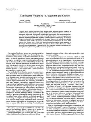
![372 A. TVERSKY, S. SATTATH, AND P. SLOVIC
faces a choice between two job offers that vary in interest and
salary. Asa natural first step, Joan examineswhether one option
dominates the other (i.e., is superior in all respects). If not, she
may try to reframe the problem (e.g., by representing the op-
tions in terms of higher order attributes) to produce a dominant
alternative (Montgomery, 1983). If no dominance emerges, she
may examine next whether one option enjoys a decisive advan-
tage: that is, whether the advantage of one option far outweighs
the advantage of the other. If neither option has a decisive advan-
tage, the decision maker seeks a procedure for resolvingthe con-
flict. Because it is often unclear how to trade one attribute
against another, a common procedure for resolving conflict in
such situations is to select the option that is superior on the
more important attribute. This procedure, which is essentially
lexicographic, has two attractive features. First, it does not re-
quire the decision maker to assess the trade-off between the at-
tributes, thereby reducing mental effort and cognitive strain.
Second, it provides a compelling argument for choice that can
be used to justify the decision to oneself as well as to others.
Consider next the matching version of the problem. Suppose
Joan has to determine the salary at which the less interesting
job would be as attractive as the more interesting one. The qual-
itative procedure described earlier cannot be used to solve the
matching problem, which requires a quantitative assessment or
a matching of intervals. To perform this task adequately, the
decision maker should take into account both the size of the
intervals (defined relative to the natural range of variation of
the attributes in question)and the relative weightsof these attri-
butes. One method of matching first equates the size of the two
intervals, and then adjusts the constructed interval according
to the relative weight of the attribute. This approach is particu-
larly compelling when the attributes are expressed in the same
units (e.g., money, percent, test scores), but it may also be ap-
plied in other situations where it is easier to compare ranges
than to establish a rate of exchange. Because adjustments are
generally insufficient (Tversky & Kahneman, 1974) this proce-
dure is likely to induce a relatively flat or uniform weighting of
attributes.
The preceding discussion is not meant to provide a compre-
hensive account of choice or of matching. It merely suggests
different heuristics or computational schemes that are likely to
be used in the two tasks. If people tend to choose according
to the more important dimension, or if they match options by
adjusting unweighed intervals, then the two procedures are
likely to yield different results. In particular, choice is expected
to be more lexicographic than matching: That is, the more
prominent attribute will weigh more heavily in choice than in
matching. This is the prominence hypothesis investigated in the
following section.
The discrepancy between choice and matching was first ob-
served in a study by Slovic (1975) that was motivated by the
ancient philosophical puzzle of how to choose between equally
attractive alternatives. In this study the respondents first
matched different pairs of (two-dimensional) options and, in a
later session, chose between the matched options. Slovic found
that the subjects did not choose randomly but rather tended
to select the option that was superior on the more important
dimension. This observation supports the prominence hypoth-
esis, but the evidence is not conclusive for two reasons. First,
the participants always matched the options prior to the choice
hence the data could be explained by the hypothesis that the
more important dimension looms larger in the later trial. Sec-
ond, and more important, each participant chose between
matched options hence the results could reflect a common tie-
breaking procedure rather than a genuine reversal of prefer-
ences. After all, rationality does not entail a random breaking
of ties. A rational person may be indifferent between a cash
amount and a gamble but always pick the cash when forced to
take one of the two.
To overcome these difficulties we develop in the next section
a method for testing the prominence hypothesis that is based
entirely on interpersonal (between-subjects) comparisons, and
we apply this method to a variety of choice problems. In the
following two sections we present a conceptual and mathemati-
cal analysis of the elicitation process and apply it to several phe-
nomena of judgment and choice. The theoretical and practical
implications of the work are discussed in the final section.
Tests of the ProminenceHypothesis
Interpersonal Tests
We illustrate the experimental procedure and the logic of the
test of the prominence hypothesis in a problem involving a
choice between job candidates. The participants in the first set
of studies were young men and women (ages 20-30 years) who
were taking a series of aptitude tests at a vocational testing insti-
tute in Tel Aviv, Israel. The problems were presented in writing,
and the participants were tested in small groups. They all agreed
to take part in the study, knowing it had no bearing on their
test scores. Some of the results were replicated with Stanford
undergraduates.
Problem I (Production Engineer)
Imagine that, as an executive of a company, you have to select be-
tween two candidates for a position of a Production Engineer. The
candidates were interviewed by a committee who scored them on
two attributes (technical knowledge and human relations) on a
scale from 100 (superb) to 40 (very weak). Both attributes are im-
portant for the position in question, but technical knowledge is
more important than human relations. On the basis of the follow-
ing scores, which of the two candidates would you choose?
Candidate A"
Candidate Y
Technical
Knowledge
86
78
[AT-63]
Human
Relations
76
91 [35%]
The number of respondents (N) and the percentage who
chose each option are given in brackets on the right side of the
table. In this problem, about two thirds of the respondents se-
lected the candidate who has a higher score on the more impor-
tant attribute (technical knowledge).
Another group of respondents received the same data except
that one of the four scores was missing. They were asked "to
complete the missing score so that the two candidates would be
equally suitable for the job." Suppose, for example, that the
lower left value (78) were missing from the table. The respon-
dent's task would then be to generate a score for Candidate Y
in technical knowledge so as to match the two candidates. The
participants were reminded that "Yhas a higher score than X
in human relations, hence, to match the two candidates Y must
have a lower score than Xin technical knowledge."](data:image/gif;base64,R0lGODlhAQABAIAAAAAAAP///yH5BAEAAAAALAAAAAABAAEAAAIBRAA7)