Final

Model based control of a
reconfigurable robot
by
Riyadh Al Saidi
A Dissertation
Submitted to the Faculty of Graduate Studies
through Mechanical, Automotive & Materials Engineering
in Partial Fulﬁllment of the Requirements for
the Degree of Doctor of Philosiphy at the
University of Windsor
Windsor, Ontario, Canada
2015
© 2015 R. Al Saidi

Model based control of a reconfigurable robot
by
R. Al Saidi
APPROVED BY:
—————————————————————–
L. Rolland, External Examiner
Department of Mechanical Engineering, Memorial University
—————————————————————–
X. Chen, External Reader
Electrical & Computer Engineering
—————————————————————–
N. Zamani, Department Reader
Mechanical, Automotive & Materials Engineering
—————————————————————–
J. Johrendt, Department Reader
—————————————————————–
B. Minaker, Supervisor
July 8th
, 2015

iii
Author’s Declaration of Originality
I hereby certify that I am the sole author of this thesis and that no part of this
thesis has been published or submitted for publication.
I certify, to the best of my knowledge, that my thesis does not infringe upon
anyone’s copyright or violate any proprietary rights and that any ideas, tech-
niques, quotations, or any other materials from the work of other people included
in my thesis, published or otherwise, are fully acknowledged in accordance with the
standard referencing practices. Furthermore, to the extent that I have included
copyrighted materials that surpasses the bounds of fair dealing within the meaning
of the Canada Copyright Act, I certify that I have obtained a written permission
of the copyright owner(s) to include such materials in my thesis and have included
copies of such copyright clearances to my appendix.
I declare that this is a true copy of my thesis, including any ﬁnal revisions, as
approved by committee and the Graduate Studies Oﬃce, and that this thesis has
not been submitted for a higher degree to any other University or Institution.

iv
Abstract
Robots with predefined kinematic structures are successfully applied to ac-
complish tasks between the robot and the environment. For more sophisticated
and future applications, it is necessary to extend the capabilities of robots, and
employ them in more complex applications, which generally require accurate and
more changeable structural properties during the interaction with the environment.
The central focus of this research was to propose a robot with new properties to
address the reconfigurability problem, including its feasible solutions using model
based control strategies. First, these reconfigurable robots have to combine as
many properties of different open kinematic structures as possible and can be
used for a variety of applications. The kinematic design parameters, i.e., their
Denavit-Hartenberg (D–H) parameters, were modeled to be variable to satisfy any
configuration required to meet a specific task. By varying the joint twist angle
parameter (a configuration parameter), the presented model is reconfigurable to
any desired open kinematic structure, such as Fanuc, ABB and SCARA robots.
The joint angle and the offset distance of the D–H parameters are also modeled
as variable parameters (a reconfigurable joint). The resulting reconfigurable ro-
bot hence encompasses different kinematic structures and has a reconfigurable
joint to accommodate any required application in medical technology, space ex-
ploration and future manufacturing systems, for example. Second, a methodology
was developed to automate model generation for n-DOF Global Kinematic Model
(n-GKM). Then, advanced model based control strategies were employed to in-
crease performance as compared to less structured approaches. An algorithm was
developed to select a relevant kinematic structural robot configuration for any pre-
defined geometric task. The main contribution of this research is that it combines
a kinematic structural design with control design methods to optimize robot capa-
bility and performance. This combination has been established by developing an
algorithm to select the optimal kinematic structure and the most applicable control
approach to perform a predefined geometric task with high tracking performance.

v
Acknowledgements
I would like to express my immense gratitude to Dr. Bruce Minaker for his
supervision and encouragement. His enthusiasm and brilliance greatly motivated
me throughout this pursuit. His support and compassion have helped me overcome
the challenging obstacles along the way.
I would also like to thank the faculty and staﬀ in the department of Mechanical
Engineering for providing interesting courses and a supportive learning environ-
ment.
I am very grateful to the the members of my defense committee. In particular,
I would like to thank Dr. X. Chen for agreeing to evaluate my work as the external
reader, and Drs. N. Zamani and J. Johrendt. The committee members provided
invaluable feedback on earlier drafts of this work. I would also like to thank Dr. Luc
Rolland for agreeing to serve as external examiner.
Ms. Angela Haskell has been an incredible source of support and I am deeply
indebted to her.
Finally, I would like to thank my ever supportive wife for standing by my side
and sharing this journey with me.

Contents
Author’s Declaration of Originality iii
Abstract iv
Acknowledgments v
List of Figures x
List of Tables xvii
Nomenclature xviii
Chapter 1. Introduction and Preliminaries 1
1.1. Introduction to Robot Kinematics 1
1.2. Introduction to Reconfigurability Theory 2
1.3. Robot Control 5
1.4. Problem Statement 10
1.4.1. General Problem Statement 10
1.4.2. Research Approach 10
Chapter 2. Development of a Reconfigurable Robot Kinematics 12
2.1. Modeling of a Reconfigurable Joint 12
2.2. Modeling of Reconfigurable Open Kinematic Robots 15
2.2.1. Spherical Wrist 16
2.2.2. Assumption 17
2.3. Reconfigurable Jacobian Matrix 17
2.3.1. Decoupling of Singularities 19
2.4. Manipulability and Singularity 20
2.4.1. Manipulability 20
2.5. Jacobian Condition and Manipulability 24
vi

CONTENTS vii
2.5.1. Joint-Space and Cartesian Trajectories 26
2.5.2. Motion Through a Singularity 27
Chapter 3. Reconfigurable Robot Dynamics 31
3.1. Reconfigurable Global Dynamic Model 31
3.2. Forward Computation for Reconfigurable Robot 32
3.3. Backward Computation of Forces and Moments 34
3.4. Development of the 3-GDM Model 38
3.4.1. Model Validation 39
3.5. Parameter Properties of a Reconfigurable Robot 45
3.5.1. Gravity Load Term 46
3.5.2. Inertia Matrix Term 47
3.5.3. Coriolis Matrix Term 49
3.5.4. Effect of Payload Term 51
Chapter 4. Linear Control 52
4.1. Optimal Robust Control 52
4.2. Mixed Sensitivity H8 Control 54
4.3. H8 Control Design 56
4.4. µ-Optimal Control 61
4.5. H8 Gain Scheduled Control 63
4.5.1. Analysis of LPV Polytopic Systems and Controllers 63
4.5.2. Synthesis of LPV Polytopic Controllers 66
4.5.3. Analysis of LPV Systems with LFT System Description 68
4.6. Linear Control Applications (Simulation Results) 70
4.6.1. Application of Mixed Sensitivity H8 Control (Simulation and
Results) 70
4.6.2. Application of H8 Control (Simulation and Results) 72
4.6.3. Application of µ-Synthesis Control and DK Iterations
(Simulation and Results) 80
4.6.4. Comparison of H8 and µ-Controllers 87
4.6.5. Order Reduction of µ Control 90
4.6.6. Application of LPV Control (Simulation and Results) 93

CONTENTS viii
Chapter 5. Nonlinear Control 97
5.1. Position Control 98
5.1.1. Link Dynamics 98
5.1.2. PD-Gravity Control 99
5.1.3. A Reconfigurable Robot with PD-Gravity Control 103
5.1.4. Three-Axis Robot Structure with PD-Gravity Control 104
5.2. Trajectory Control 108
5.2.1. Feedback Linearization Control 108
5.2.2. Input-Output Linearization 109
5.2.3. Sliding Mode Control (SMC) 112
5.2.4. Sliding Mode Control Based on Estimated Model 114
5.2.5. Simulation of 3-DOF Reconfigurable Manipulator 117
5.2.6. Sliding Mode Control Based on Bounded Model 120
5.2.7. Sliding Mode Control Based on Computed Torque Method 123
5.2.8. Adaptive Control 126
5.2.9. Derivation of Adaptive Sliding Mode Control 127
5.2.10. Simulation Results of 3-DOF Reconfigurable Robot 129
Chapter 6. Kinematic and Control Selection Algorithm 132
6.1. Configuration Phase 132
6.1.1. Internal D–H Parameters Optimization 133
6.2. Control Phase 134
6.2.1. Dynamic Parameter Properties 136
6.2.2. The Reconfigurable Control Algorithm 136
6.3. Algorithm Implementation (Simulations and Results) 141
6.3.1. Trajectory of Two Circles in Joint Space Motion 141
6.3.2. Straight Line Trajectory in Joint Space 144
6.3.3. Position (Linear) and Trajectory (Nonlinear) Control Method
Selection 148
6.4. Comparison between Linear and Nonlinear Control Approaches 156
6.5. Summary 157
Chapter 7. Conclusions and Recommendations 159

CONTENTS ix
7.1. Conclusions 159
7.2. Recommendations 162
Appendix A: Bosch Scara Model 164
Appendix B: Bosch Scara Model 166
Appendix C: Kinematic Calculations 168
References 169
Vita Auctoris 175

List of Figures
1.1 Definition of standard Denavit and Hartenberg (D–H) parameters.
Source; Manseur, [63]............................................................................ 2
1.2 Set of design variables of the 3-DOF configuration modular robots,
this set is a commercial product of AMTEC GmbH Company. Source;
I.M. Chen, [22]...................................................................................... 4
1.3 Mechanical set up of a modular and reconfigurable robot (left). The
ICT power cube Mechatronical component (right). Source; Strasser,
[84]........................................................................................................ 5
1.4 Robotic system with motion control system, inner and outer loop
controllers.............................................................................................. 6
1.5 Standard robust control problem. ......................................................... 9
2.1 Kinematic structures of the ABB and Stanford robots, D–H param-
eters are from sources; Dawson, [57] and Spong, [80]........................... 15
2.2 The spherical wrist, joint axes 4, 5 and 6. ............................................ 16
2.3 All possible configuration models of a reconfigurable hybrid joint........ 18
2.4 Workspace of RRR Configuration with four different twist angle val-
ues π{16, π{8, π{4, and π{2. ................................................................. 21
2.5 Workspace of RRT Configuration with different link lengths 0.15, 0.3
and 0.45 m. ........................................................................................... 22
2.6 3D profile of the manipulability index measure of RRR configuration. 23
2.7 3D profile of the manipulability index measure of RRT configuration.. 24
2.8 Cartesian velocity ellipsoid of RRR configuration with different twist
angle values of pπ{16, π{6, π{2q degrees................................................. 26
2.9 Cartesian velocity ellipsoid of RRT configuration with different pris-
matic lengths of 0.1, 0.2 and 0.3 m. ...................................................... 27
x

LIST OF FIGURES xi
2.10 Joint angles during joint-space motion (left). Cartesian coordinates
of the end-effector in x, y and z directions (right)................................ 28
2.11 Cartesian position locus in the xy-plane (left). Euler angles roll-
pitch-yaw versus time (right). ............................................................... 28
2.12 Joint angles during Cartesian motion (left). Cartesian coordinates of
the end-effector in x, y and z directions (right).................................... 28
2.13 Cartesian position locus in the xy-plane (left). Euler angles roll-
pitch-yaw versus time (right). ............................................................... 29
2.14 Joint angles follow Cartesian path through a wrist singularity (left),
joint angles follows joint-space path (right). ......................................... 29
2.15 Manipulability measure of Cartesian and joint-space paths.................. 30
3.1 RR planar kinematic structure.............................................................. 40
3.2 RT planar kinematic structure.............................................................. 41
3.3 TR planar kinematic structure.............................................................. 42
3.4 TT planar kinematic structure.............................................................. 42
3.5 Scara kinematic structure. .................................................................... 44
3.6 The workspace of a predefined kinematic structure of the PUMA 560. 46
3.7 The workspace of a reconfigurable manipulator.................................... 47
3.8 Gravity load variation with a reconfigurable manipulator pose (shoul-
der gravity load).................................................................................... 48
3.9 Gravity load variation with a reconfigurable manipulator pose (Elbow
gravity load).......................................................................................... 48
3.10 Variation of inertia matrix elements M11 with configuration................ 49
3.13 Joint 2 inertia as a function of joint 3 angle, M22pq3q........................... 50
4.1 Closed loop configuration with mixed sensitivity consideration............ 53
4.2 General H8 control configuration. ........................................................ 55
4.3 S/SK mixed sensitivity optimization in regulation form (left), S/SK
mixed sensitivity minimization in tracking form (right). ...................... 57
4.4 Uncertain system representation........................................................... 57

LIST OF FIGURES xii
4.5 Standard H8{µ control structure (left), A control structure for closed
system analysis (right). ......................................................................... 58
4.6 A control configuration with extended uncertainty structure. .............. 61
4.7 µ-Synthesis Control Procedure.............................................................. 62
4.8 The structure of the LPV system and control using Linear Fractional
Transformation (LFT) description system. ........................................... 68
4.9 Model of first two links and servo motors of the Bosch Scara robot..... 71
4.10 Schematic top view of the Bosch Scara robot in null position. ............. 71
4.11 Inverse of performance weight (dashed line) and the resulting sensi-
tivity function (solid line) for two H8 designs (1 and 2) for distur-
bance rejection. ..................................................................................... 73
4.12 Closed loop step responses for two alternative designs (1 and 2) for
disturbance rejection problem. .............................................................. 73
4.13 Derived block diagram of the first link of the Bosch Scara robot. ........ 74
4.14 LFT representation of the perturbed Bosch Scara model ..................... 75
4.15 Perturbed (set of family) open loop systems......................................... 75
4.16 Singular value of the closed loop with H8 controller............................ 76
4.17 H8 control structure............................................................................. 77
4.18 Sensitivity and performance weighting function with H8 controller..... 78
4.19 Robust stability analysis with H8 control. ........................................... 78
4.20 Nominal and robust performance with H8 control............................... 79
4.21 Perturbed (set of family) of closed loop systems with different uncer-
tainty values.......................................................................................... 80
4.22 Transient response to reference input with H8 control......................... 80
4.23 Transient response to disturbance input with H8 control. ................... 81
4.24 Sensitivity and weighting functions of Mu-Control............................... 83
4.25 Robust stability of Mu-control.............................................................. 83
4.26 Nominal and robust performance of Mu-Control. ................................. 83
4.27 Sensitivity functions of perturbed systems with Mu-Control................ 84
4.28 Performance of perturbed systems with Mu-Control. ........................... 84
4.29 Frequency responses of perturbed closed loop systems with Mu-Control. 85
4.30 Transient response to step reference input with Mu-Control. ............... 86

LIST OF FIGURES xiii
4.31 Transient response to disturbance input with Mu-Control. .................. 86
4.32 Transient responses of perturbed closed loop with Mu-Control............ 86
4.33 Frequency responses of H8 and µ-controllers. ...................................... 87
4.34 Frequency responses of closed loop systems.......................................... 88
4.35 Comparison of robust stability of H8 and µ-controllers. ...................... 88
4.36 Comparison of nominal performance of H8 and µ-controllers.............. 89
4.37 Comparison of robust performance of H8 and µ-controllers................. 89
4.38 Performance degradation of H8 and µ-controllers................................ 90
4.39 Frequency responses of full and reduced order controllers. ................... 92
4.40 Transient response for reduced order controller. ................................... 93
4.41 LPV control structure includes the LPV system Ppθptqq, performance
weighting functions Wp, robustness function Wu, and LPV polytopic
controllers (K1pθptqq, ¨ ¨ ¨ , K3pθptqq and input filter Wf ......................... 94
4.42 Parameter trajectory. ............................................................................ 96
4.43 Step response of the LPV closed loop system. ...................................... 96
5.1 Performance of PD-gravity controller, RR configuration; tracking
step position of joint 1 (left), motor torque (right)............................... 104
step position of joint 2 (left), motor torque (right)............................... 105
step position error joint 1 (left), tracking position error joint 2 (right).105
5.4 Performance of PD-gravity controller, RT configuration; tracking po-
sition of prismatic joint 2 (left), motor torque (right)........................... 106
5.5 RRT configuration (Scara); tracking circular path of joint 1 (left),
motor torque of joint 1 (right). ............................................................. 107
5.6 RRT configuration (Scara); tracking circular path joint 2 (left), motor
torque of joint 2 (right)......................................................................... 107
5.7 RRT configuration (Scara); tracking circular path error joint 1 (left),
tracking circular path error joint 2 (right). ........................................... 108
5.8 Motor torques of joints 1 and 2 using control law (211); the chattering
is due to the sign function..................................................................... 118

LIST OF FIGURES xiv
5.9 Motor torques of joints 1 and 2 when replacing the function sgnpsq
with satps{Φq. ....................................................................................... 119
5.10 Tracking positions of joints 1 and 2 using the control law (209.) Ref-
erence position (solid), actual position (dotted).................................... 119
5.11 Tracking velocities of joints 1 and 2 using the control law (209.)
Reference velocity (solid), actual position (dotted)............................... 120
5.12 The phase portrait of the trajectory errors of joints 1 and 2................ 120
5.13 Motor torques of joints 1 and 2 using control law (217); the chattering
is due to the sign function..................................................................... 121
5.14 Motor torques of joints 1 and 2 when replacing the function sgnpsq
with satps{Φq. ....................................................................................... 122
5.15 Tracking positions of joints 1 and 2 using control law (209). Reference
position (solid), actual positions (dotted). ............................................ 122
5.16 Tracking velocities of joints 1 and 2 using control law (209). Reference
velocities (solid), actual positions (dotted). .......................................... 123
5.17 The phase portrait of the trajectory errors of joints 1 and 2................ 123
5.18 Tracking positions of joints 1 and 2 using the control law (219). Ref-
erence position (solid), actual positions (dotted). ................................. 125
5.19 Motor torques of joints 1 and 2 using the control law (224), replacing
the function sgnpsq with satps{Φq......................................................... 125
5.20 Trajectory errors of joints 1 and 2. ....................................................... 126
5.21 Control structure diagram of the adaptive control................................ 127
5.22 Tracking position of the joint 1 to a trigonometric function (above),
reference position (solid) and actual position (dotted). The tracking
error (central), and the control torque (below). .................................... 130
5.23 Tracking position of the joint 2 to a trigonometric function (above),
reference position (solid) and actual positions (dotted). The tracking
error (central), and the control torque (below). .................................... 130
5.24 The normalized values of the inertia parameters ϕ1 (above) and ϕ2
(below). ................................................................................................. 131
5.25 The normalized values of the inertia parameters ϕ3 (above) and ϕ4
(below). ................................................................................................. 131

LIST OF FIGURES xv
6.1 Configuration phase. ............................................................................. 133
6.2 Control phase. ....................................................................................... 135
6.3 A comprehensive algorithm for configuration and control of a recon-
figurable robot....................................................................................... 140
6.4 A reconfigurable robot follows a trajectory motion (lower and upper
circles)................................................................................................... 142
6.5 The joint coordinates of a reconfigurable robot during the joint space
path....................................................................................................... 143
6.6 Cartesian position (x,y,z) of the end effector during the joint space
trajectory............................................................................................... 143
6.7 The Euler angles (roll, pitch, yaw) of the end effector.......................... 144
6.8 Manipulability of the reconfigurable robot following a joint space
trajectory............................................................................................... 144
6.9 Front view of the workspace in the xz-plane of a reconfigurable robot. 146
6.10 End effector motion from pose (0.4064, 0.5,0.3303) to (0.8032, 0.5,0.3303).146
6.11 Joint coordinates motion versus time.................................................... 147
6.12 Cartesian position of the end effector versus time. ............................... 147
6.13 Cartesian position of the trajectory in the xy-plane versus time.......... 148
6.14 Euler angles, roll-pitch-yaw of the end effector versus time. ................. 148
6.15 Performance weighting function of the sensitivity function S “ 1
p1`GKq
150
6.16 Step response of H8-control.................................................................. 150
6.17 Disturbance response using H8-control. ............................................... 151
6.18 Frequency response of a weighted sensitivity function S “ 1
p1`GKq
....... 152
6.19 Step response of 20 frozen parameters using gain-scheduled controller. 152
6.20 Gain-scheduled control amplitude......................................................... 153
6.21 Tracking error using gain-scheduled control.......................................... 153
6.22 Trajectory tracking for a trigonometric reference command using
SMC method......................................................................................... 154
6.23 Tracking error for unknown parameters using SMC method. ............... 155
6.24 Trajectory tracking for a trigonometric function using the adaptive
control method...................................................................................... 155

LIST OF FIGURES xvi
6.25 Tracking error for time varying dynamic parameters using adaptive
control method...................................................................................... 156

List of Tables
2.1 D–H parameters of the n-GKM model.................................................. 12
2.2 D–H of a spherical wrist, source; Spong, [80]. ...................................... 17
2.3 D–H parameters of the ABB manipulator robot, source; Spong, [80]. . 21
2.4 D–H parameters of the Stanford manipulator robot, source; Spong,
[80]........................................................................................................ 23
3.1 Reconfiguration parameters values........................................................ 37
3.2 Reconfigurable D–H parameters of the 3-GKM model.......................... 39
3.3 Kinematic initial parameters of 2-DOF RR configuration .................... 40
3.4 Dynamic initial parameters of 2-DOF RR configuration ...................... 40
3.5 Kinematic initial parameters of 2-DOF RT configuration..................... 41
3.6 Dynamic initial parameters of 2-DOF RT configuration....................... 41
3.7 Kinematic initial parameters of 2-DOF TR configuration .................... 42
3.8 Dynamic initial parameters of 2-DOF TR configuration ...................... 42
3.9 Kinematic initial parameters of 2-DOF TT configuration .................... 43
3.10 Dynamic initial parameters of 2-DOF TT configuration....................... 43
3.11 Kinematic initial parameters of 3-DOF SCARA configuration............. 43
3.12 Dynamic initial parameters of 3-DOF SCARA configuration ............... 44
3.13 D–H parameters of the PUMA 560 Manipulator, source; Fu, [41]........ 46
6.1 Dynamic parameter properties of a reconfigurable robot...................... 136
A.1 Nominal parameter values of the Bosch Scara robot arm ..................... 166
A.2 Nominal parameter values of the Bosch Scara robot arm ..................... 166
A.3 Different values for inertias and damping for different joint position
of link 2 (left). Estimated parameter values for stiction and Coulomb
friction (right). ...................................................................................... 167
xvii

Nomenclature
Lmi Inductance of motor coil of joint i rHs
Li Size of the Link i rHs
Rmi Impedance of motor armature, included wires of joint i rΩs
Kmi Servo motor constant of joint i rN m{As
Jmi Inertia of servo motor of joint i rkgm2
s
JLi Inertia of the Link i rkgm2
s
Ji Total inertia of Link i rkgm2
s
Jc Cross-coupling inertia between joints rkgm2
s
Fvi Viscous friction of joint i rN ms{rads
FvL Viscous friction in mechanical link 1 rN ms{rads
Fvm Viscous friction in Servo motor of joint 1 rN ms{rads
Fci Coulomb friction of joint i rN ms
Fsi Static friction (Stiction) of joint i rN ms
KP i1 Proportional constant of tacho controller in Servo Amplifier i r1s
KIi1 Integration constant of tacho controller in Servo Amplifier i rs´1
s
KPi2 Proportional constant of current controller in Servo Amplifier i rV {As
KIi2 Integration constant of current controller in Servo Amplifier i rV {Ass
Ti Time constant of Tacho controller in Servo Amplifier i rs´1
s
ml Load mass rkgs
KS Spring constant rN m{rads
DS Damper constant rN ms{rads
xviii

NOMENCLATURE xix
θmi Position of motor axis of joint i rrads
θi Position of joint axis i rrads
9θmi Velocity of motor axis of joint i rrad{ss
9θi Velocity of joint axis i rrad{ss
:θi Acceleration of joint axis i rrad{s2
s
C1 Cospθ1q
S1 Sinpθ1q
C12 Cospθ1 ` θ2q
S12 Sinspθ1 ` θ2q
N1 Gear ratio r1s
τLD,i Disturbance torques on joint i rN ms
δADi Quantization error of sensor joint i rrads
δDA Resolution of DA-converter rV s
δF Perturbation in friction rN ms{rads
δ1{J Perturbation in inertia r1{kgm2
s
δθ Tracking error rrad{ss
p1 Interconnection output to inertia error rN ms
p2 Interconnection output to friction error rrad{ss
q1 Interconnection input to inertia error rN{kgms
q2 Interconnection input to friction error rN ms
US Input voltage to Servo motor [V ]
USA Input voltage to Tacho controller of Ampliﬁer System rV s
ISA Input current to Current controller of Ampliﬁer System rAs
h Sample time [s]
W∆ Scaling function for perturbation matrix

NOMENCLATURE xx
WP Weighing function of tracking error (Performance Spec)
Wθ Scaling function for velocity set point
Wτ Scaling function for disturbance torque
WDA Scaling function for Ampliﬁer set point
WF Scaling of Friction perturbation
WJ Scaling of inertia perturbation
K Controller
B Set of all normed perturbation matrices with σmaxp∆q ď 1
M Closed-loop interconnection matrix
M1
Open-loop interconnection matrix
∆ Noise-block, built of ∆1 and ∆P
∆1 Perturbation transfer matrix (structured)
∆P Block structure appended to ∆ for robust performance calculations
d Input signals
e Tracking error
c Controller signal
w Input of perturbation matrix 1 into the interconnection matrix
z Output of the interconnection matrix to the perturbation matrix 1

CHAPTER 1
Introduction and Preliminaries
1.1. Introduction to Robot Kinematics
A serial-link manipulator comprises a set of bodies called links connected in a
chain by joints. Each joint has one degree of freedom, either translational (sliding
or prismatic joint) or rotational (revolute joint). To describe the rotational and
translational relationships between adjacent links, Denavit and Hartenberg pro-
posed a matrix method of systematically establishing a coordinate frame to each
link of an articulated chain. The Denavit-Hartenberg (D–H) representation [35]
results a 4ˆ4 homogeneous transformation matrix representing each link’s coordi-
nate frame at the joint with respect to the previous link’s coordinate frame. To
analyze the motion of robot manipulator, coordinate frames are attached to each
link starting from frame F0, attached to the base of the manipulator link, all the
way to the frame Fn, attached to the robot end-effector as shown in Figure 1.1.
Every coordinate frame is determined and established on the basis of three rules:
(1) The zi´1 axis lie along the axis of motion of the ith joint.
(2) The xi axis is normal to the zi´1 axis.
(3) The yi axis completes the right-handed coordinate system as required.
As the frames have been attached to the links, the following definitions of the
link (D–H) parameters are valid:
‚ Joint angle θi is the angle around zi´1 that the common perpendicular
makes with vector xi´1.
‚ Link offset di is the distance along axis zi´1 to the point where the common
perpendicular to axis zi is located.
‚ Link length ai is the length of the common perpendicular to axes zi´1 and
zi.
‚ Link twist αi is the angle around xi that vector zi makes with vector zi´1.
1

1.2. INTRODUCTION TO RECONFIGURABILITY THEORY 2
Figure 1.1. Definition of standard Denavit and Hartenberg (D–H)
parameters. Source; Manseur, [63].
For a rotary joint, di, ai, and αi are the joint parameters and remain constant
for a robot, while θi is the joint variable that changes when link i rotates with
respect to link i ´ 1. For a prismatic joint, θi, ai, and αi are the joint parameters
and remain constant for a robot, while di is the joint variable.
1.2. Introduction to Reconfigurability Theory
Robotics technology has been recently exploited in a variety of areas and var-
ious robots have been developed to accomplish sophisticated tasks in different
fields and applications such as in space exploration, future manufacturing sys-
tems, medical technology, etc. In space, robots are expected to complete different
tasks, such as capturing a target, constructing a large structure and autonomously
maintaining in-orbit systems. In these missions, one fundamental task with the
robot would be the tracking of changing paths, the grasping and the positioning
of a target in Cartesian space. To satisfy such varying environments, a robot with
changeable configuration (kinematic structure) is necessary to cope with these
requirements and tasks. Another field of technology is the new manufacturing en-
vironment, which is characterized by frequent and unpredictable market changes.
A manufacturing paradigm called Reconfigurable Manufacturing Systems (RMS)
was introduced to address the new production challenges [52]. RMS is designed
for rapid adjustments of production capacity and functionality in response to new

circumstances, by rearrangement or change of its components and machines. Such
new systems provide exactly the capacity and functionality that is needed, when
it is needed [39]. The rapid changes and adjustments of the RMS structure must
happen in a relatively short time ranging between minutes and hours and not days
or weeks. These systems’ reconfigurability calls for their components, such as ma-
chines and robots to be rapidly and efficiently modifiable to varying demands [48].
Robot manipulators working in extreme or hazardous environments (biological,
chemical, nuclear,..., etc.) often need to change their configuration and kinematic
structures to meet the demands of specific tasks. It is desirable and cost effective
to employ a single versatile robot capable of performing tasks such inspection,
contact operations, assembly (insertion or removal parts), and carrying objects
(pick and place). Robots with maximum manipulability are well conditioned for
dexterous contact tasks [16, 61] and configurations that maximize the robot links
and distance from the environment are suitable for payload handling [56]. The
optimization of a robot workspace over its link lengths, as the design parameters,
is reported in [55, 47], while optimization of kinematic parameters and criteria
for fault tolerance are discussed in [50].
In the literature, modular robotic structures are presented as a solution to cope
with reconfigurable structure of robots. A modular reconfigurable robot consists
of a collection of individual link and joint components that can be arbitrarily as-
sembled into a number of different geometries. Such a system can provide agility
to the user to cope with a wide spectrum of tasks through proper selection and
reconfiguration of a large inventory of functional components. Several prototyping
systems have been demonstrated in various research institutions, [87], [42], [67]
and [13]. An automated generation of D–H parameters methodology has devel-
oped for the modular manipulators [22]. The authors derived the kinematic and
dynamic models of reconfigurable robots using D–H parameters for different sets of
joints, links and gripper modules as shown in Figure 1.2. Furthermore, a library of
modules is formed from which any module can be called with its associated kine-
matic and dynamic models. In [58], a modular and reconfigurable robot design
is introduced with modular joints and links. The proposed design introduces zero

Figure 1.2. Set of design variables of the 3-DOF configuration
modular robots, this set is a commercial product of AMTEC GmbH
Company. Source; I.M. Chen, [22].
link offsets to increase the robot’s dexterity and maximize its reachability. A mod-
ular and reconfigurable robot (MRR) with multiple working modes was designed
[59]. In the proposed MRR design, each joint module can independently work
in active modes with position or torque control, or passive modes with friction
compensation. With the MRR, the joint module was designed as a hybrid joint
in working modes and not in the sense of mechanical motion. A reconfigurable
robot was proposed [5] and achieves the reconfigurability by utilizing passive and
active joints. In [21], an automated approach was presented to build kinematic
and dynamic models for assembled modular components of robots. The developed
method is applicable to any robotic configuration with a serial, parallel or hybrid
structure. Reconfigurable plug and play robot kinematic and dynamic modeling
algorithms are developed [22]. These algorithms are the basis for the control and
simulation of reconfigurable modular robots. The reconfigurable robot (RRS) was
regarded as a modular system [20]. A task-based configuration optimization based
on a generic algorithm was used to solve a predefined set of joint modules for spe-
cific kinematic configuration. A modular and reconfigurable robot for industrial

1.3. ROBOT CONTROL 5
Figure 1.3. Mechanical set up of a modular and reconfigurable
robot (left). The ICT power cube Mechatronical component (right).
Source; Strasser, [84].
purposes has been introduced [84]. The PROFACTOR GmbH has presented a
modular and reconfigurable robot with power cube (Mechatronical Components)
modules depicted in Figure 1.3. These modules were designed to be identical and
self-contained with actuation, memory, and mechanical, electrical and embedded
programming. A reconfigurable robot has been introduced by [36] that unifies the
kinematic structure of industrial robots. In that unification process, eight mod-
ules were reconfigured by changing configuration parameters. These parameters
represent the trigonometric functions of the robot twist angles.
The main drawbacks of the modular robots proposed in the literature are the
high initial investment necessary in modules that remain idle during many activi-
ties, and the significant lead time for replacement, attachment and detachment of
the components prior to performing a specific task.
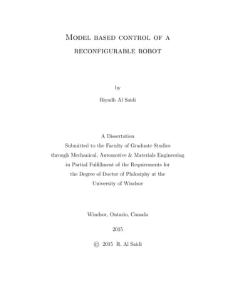
1.3. Robot Control
The use of advanced robot control laws may contribute significantly to improve
the robot functions and properties. The improvement of the robot design itself
can also contribute substantially to the desired increase in performance and capa-
bilities. The combination of the controller with proper sensors can provide some

sense and awareness of the environment, and improve its accuracy and speed as
well.
Robotic
Arm
Actuator
DC Motor
Outer Loop
Controllers
PD, PID
/H 
,q q
, ,d d dq q q 
Trajectory
Generation
,q qu
Robotic SystemMotion Control System
Host
Inner Loop
Feedback
Linearization
Controller
Figure 1.4. Robotic system with motion control system, inner and
outer loop controllers.
The former and current problems in the robotics application fields has affected
the research of robot control in a number of fundamental topics: modeling, position
control, robust control and motion planning. This has motives research in robot
modeling, simulation and control design. Therefore, position and trajectory control
is an important research field in robotics control. The position/motion control
problem has received a great deal of interest in robotics. Therefore, a survey that
covers the important control strategies is given with examples and applications.
PD and PID Control
The PD (Proportional-Derivative) and PID (Proportional-Derivative-Integral) con-
trollers are the most applied in industry, which is also true for robotics. Some
references propose a high gain PD controller to ensure global stabilization of the
robot [68, 69, 71], which is unsuited for practical applications due to excitation
of unavoidable higher dynamics and excessive noise amplification. PID controllers
are more suitable to eliminate the steady state error of the final position response.
These controllers introduce an integration action to the resulting closed loop im-
proving the performance tracking requirements.
Feedback Linearization Control
The application of feedback linearization theory to solve robotics control prob-
lems has led to the computed torque approach. Feedback linearization control

methods are inner-outer loop control methods: the inner loop must linearize the
plant, whereas the outer loop must achieve the desired closed loop requirements.
Figure 1.4 shows the control motion structure (inner and outer control loops) of a
robot driven by a DC motor. The term Computed Torque Control (CTC) is the
application of PD control at the outer loop to a linearized system by the feedback
linearization control. In robotics, CTC is used to apply PD controllers at the outer
loop independently (every joint controlled separately) [53]. There are two impor-
tant features of the feedback linearization method that require attention: model
error and the outer loop controller design. Feedback linearization is based on the
exact model of the system. Therefore, the controller may be sensitive to modeling
errors such as parameter errors and unmodeled dynamics. Parameter uncertainty
is commonly addressed by either robust control methods or by the derivation of
adaptive controllers [66, 77]. In particular, when a restricted amount of parame-
ters must be estimated (in case of an unknown load), adaptive controllers can be a
suitable approach. The feedback linearization control actively linearized the plant,
such that the resulting system can be considered as a linear system. Therefore,
it is possible to apply one of many linear control methods to close the loop and
achieve the required performance. As a result, a large number of controllers for
the outer loop control are proposed: the standard PD loop of CTC, linear optimal
control [83, 78], sliding mode control, and H8{µ robust optimal controllers.
Lyapunov Based Control
An important tool for control of rigid body systems is Lyapunov stability theory,
which based on the strict dissipation of a suitable energy function [76]. Although
this theory is not constructive to design a controller, a simple structure of the equa-
tions of motion with some relevant assumptions allow a derivation of stabilizing
controllers. These assumptions may include bounded disturbances and bounded
parameter variations. The passivity based control approach attempts to reshape
the robot energy function, rather than imposing a completely diﬀerent behavior
as with the CTC approach [14, 19]. Experiments have shown and indicated the

passivity controllers are more robust than CTC. Another result of Lyapunov sta-
bility theory is the sliding mode control (SMC), which is considered to be a robust
control approach.
Robust Control
To ensure a suitable behavior of the closed loop robot, even in the presence of
modeling errors and disturbances, it is desired to design controllers that are ro-
bust with respect to these errors and disturbances. Modeling errors are generally
separated into parameter errors and unmodeled dynamics, which may have differ-
ent affect on the closed loop system. The standard control framework, adopted in
many textbooks on modern control [23, 60, 88], is shown in Figure 1.5. A con-
troller Kpsq is provided with measurement signals y and has to stabilize a plant
Ppsq with input signals u such that the cost variables z are minimal in some sense,
despite the disturbance signals w and the parametric and dynamic uncertainties
represented in ∆psq. The plant Ppsq is often called the generalized plant or stan-
dard plant since it usually does not only consist of the plant to be controlled, but
can also contain weightings, e.g., parametric and dynamic uncertainty weighting,
input signal thresholds, and the robot dynamic model to be simulated. Also the
other entities can be viewed in a generalized way, e.g., reference signals can be
incorporated as disturbances w and additional feedback paths can be taken in
case of a robust control problem to describe a set of systems, i.e., uncertainty.
A survey can be found covering a number of robust robot position controller de-
sign methods: passivity control, sliding mode control and linear robust control by
factorization approach in [82]. The most popular robust control design method
in robotics literature is the sliding mode control (SMC), also known as Variable
Structure Switching (VSS) control. Sliding mode control is commonly used to ad-
dress parameter uncertainty and bounded disturbances [76, 86]. As mentioned,
SMC is based on upon Lyapunov stability theory, and basically tries to determine
the nominal feedback control law and a corrective control action that steers the
controlled system to the desired behavior, defined as the ‘sliding surface’.

yu
w z
( )K s
( )P s
( )s
yu
Figure 1.5. Standard robust control problem.
Optimal Control
Apart from the application of linear outer loop control applied to the feedback
linearized robot, there have been some attempts made to apply optimal control
directly to the rigid body dynamics. The main problem with these approaches
is the amount of assumptions and choices that have to be made to allow for a
solution. For example in [30], an optimal quadratic control is considered with a
special choice optimization criterion, which results in a nonlinear PID controller.
Another example in [44], where an H8-optimal control problem is considered,
results in a nonlinear static state feedback PD controller. Following these methods
to construct a nonlinear controller does not allow the versatility required for a
controller design method needed to solve real-world problems.
The reason is that currently the nonlinear control theory cannot provide a
general robust controller design methodology, due to high complexity of both the
robot model and the involved design specifications. General cases addressed with
optimal control infrequently allow a closed solution, and one has to resort to com-
putationally intensive numerical methods. In the case of special properties of the
uncertainty, e.g., signal roundedness, there do exist applicable controller design
methods, e.g., sliding mode control. These control methods have restricted appli-
cabilities as they cannot exploit structural knowledge of the uncertainty. Linear
control theory does have that capability e.g. H8{µ controller design methods have
limited means of specifying the desired properties of the closed loop system. Linear
control theory also has its limits, but offers a larger variety of specifications.

1.4. PROBLEM STATEMENT 10
1.4. Problem Statement
Current robot structures have physical limitations with respect to their configu-
rations and capabilities. They are preconfigured to do specific tasks. For example:
a robot structure with 5-DOF (3R-2T) would have three revolute (rotational mo-
tion) and two prismatic (translational motion) joints with fixed coordinate frames
that cannot be automatically changed to any other configuration. The structure
of most robots can be changed only by physically replacing their joints or links
(modules). These limitations are reflected on the robot’s path, workspace, inertia,
torque, power concept,..., etc., making them unsuitable for future RMS.
1.4.1. General Problem Statement
The aforementioned leads to the following problem statement for this research:
Propose a robot with new properties to address the reconfigurabil-
ity problem, including its feasible solutions using model based control
strategies.
1.4.2. Research Approach
Structural robot design and control methods are combined to solve the reconfig-
urability problem. A rotational/translational reconfigurable joint is investigated
to add new properties necessary to extend the robot capabilities in performing
more sophisticated tasks. The D–H parameters of a reconfigurable robot will be
regarded as variable to describe all possible kinematic configurations. A Global
Kinematic Model (GKM) is developed based on specific reconfigurable parameters
to automate generation models for any robot configuration. Then, an automatic
generation of dynamic equations using the Global Dynamic Model (GDM) is con-
structed to auto-generate the equations of motion of any specified configuration.
The recursive Newton-Euler algorithm is employed to generate the dynamic ele-
ments: the inertia matrix, Coriolis torque matrix, centrifugal torque matrix, and
the gravity torque vector. The parameters of a reconfigurable robot are often
unknown, nonlinear or uncertain. Moreover, most of these parameters are time
varying, position and orientation (pose) dependent. Consequently, the following
control strategies were explored and analyzed thoroughly:

1.4. PROBLEM STATEMENT 11
‚ Nonlinear PD-Gravity control.
‚ Optimal robust control such as H8{µ controllers.
‚ Gain Scheduling control.
‚ Sliding Mode Control (SMC).
‚ Adaptive control.
Based on the dynamic parameter types, a reconﬁgurable control algorithm is devel-
oped, which leads to optimize the control method selection for a speciﬁc kinematic
structure.

CHAPTER 2
Development of a Reconfigurable Robot Kinematics
A development of the general n-DOF Global Kinematic Model (n-GKM) is
necessary for supporting any open kinematic robotic arm, and possible redundant
kinematic structures that are intended to support more than 6-DOF. The n-GKM
model is generated by the D–H parameters, given in Table 2.1 and as proposed by
Djuric, Al Saidi, and ElMaraghy [37]. All D–H parameters presented in the Table
2.1 are not fixed values; they are modeled as variables to satisfy the properties of
all possible open kinematic structures of a robotic arm. The twist angle variable
αi is limited to five different values, (00
, ˘900
, ˘1800
), to maintain perpendicular-
ity between joints’ coordinate frames. Consequently, each joint has six different
positive directions of rotations and/or translations.
Table 2.1. D–H parameters of the n-GKM model.
i di θi ai αi
1 R1dDH1 ` T1d1 R1θ1 ` T1θDH1 a1 00
, ˘1800
, ˘900
2 R2dDH2 ` T2d2 R2θ2 ` T2θDH2 a2 00
, ˘1800
, ˘900
. . . . . . . . . . . . . . .
3 RndDHn ` Tndn Rnθn ` TnθDHn an 00
, ˘1800
, ˘900
The subscript DHn implies that the di or θi parameter is constant.
2.1. Modeling of a Reconfigurable Joint
The reconfigurable joint is a hybrid joint that can be configured to be a revolute
or a prismatic type of motion, according to the required task. For the n-GKM
model, a given joint’s vector zi´1 can be placed in the positive or negative directions
of the x, y, and z axis in the Cartesian coordinate frame. This is expressed in
Equations (1)-(2):
12

2.1. MODELING OF A RECONFIGURABLE JOINT 13
Rotational Joints : Ri “ 1 and Ti “ 0 (1)
Translational Joints : Ri “ 0 and Ti “ 1 (2)
The variables Ri and Ti are used to control the selection of joint type (rotational
and/or translational). The orthogonality between the joint’s coordinate frames is
achieved by assigning appropriate values to the twist angles αi. Their trigonomet-
ric function are defined as the joint’s reconfigurable parameters (KSi & KCi) and
expressed in Equations (3)-(4):
Ksi “ sinpαiq (3)
Kci “ cospαiq (4)
To construct a reconfigurable joint, all six different positive directions of rotations
or translations must be included. The procedure will start from the first coordi-
nate frame by defining the orientation of the vector, Z0. Because there are six
combinations of vector Z0, the process starts from the first one, named Z1
0 . The
selection of vector Z1
0 , can be combined with four more orientations of vectors X0
and Y0. They are: X11
0 , Y 11
0 , X12
0 , Y 12
0 , X13
0 , Y 13
0 , X14
0 , Y 14
0 . The second combina-
tion of Z1
0 and its X0 and Y0 includes the new vector Z2
0 and the four combinations:
X21
0 , Y 21
0 , X22
0 , Y 22
0 , X23
0 , Y 23
0 , X24
0 , Y 24
0 . Similarly, all other possible combinations
of different Z1
0 and the X0 and Y0 vectors. This will produce a reconfigurable
joint having 24 different possible coordinate frames. Thus, a reconfigurable joint
model includes 6R and 6T different types of motion, which is the maximum num-
ber of motions that can be produced in 3D space. The following five definitions
are developed for proper use of the model.
Definition 2.1. The degree of the joints reconfigurability, RJ can be between
2 and 12. This parameter defines the level of the joints reconfigurable capabilities,
Equation (5).
2 ď Rj ď 12 (5)

2.1. MODELING OF A RECONFIGURABLE JOINT 14
Definition 2.2. Similarly, the links reconfigurable parameter, RL, which is
simply the changeable link length, and can be any real number.
RL P R (6)
Definition 2.3. For any joint to be reconfigurable, the following condition
must be satisfied: the number of different motions should be a minimum of two,
Equation (7).
minpRjq “ 2 (7)
From those three definitions a clear description of the reconfigurable robot is
achieved.
Definition 2.4. The robot is reconfigurable if and only if it has a minimum
of one reconfigurable joint or link.
Definition 2.5. The n-DOF Global Kinematic Model (n-GKM) is a recon-
figurable model because it has all reconfigurable joints and links. Its joints satisfy
the maximum number of reconfigurations pRj “ 12q
The n-GKM model starts from the base frame, which represents the coordi-
nate frame px0, y0, z0q of the first joint, and has six possible frames for the second
joint, presented with coordinate frame px1, y1, z1q. From the second joint coordi-
nate frame px1, y1, z1q, there are again six different combinations for joint three’s
coordinate frame px2, y2, z2q, and so on, up to the flange frame pxn, yn, znq.

2.2. MODELING OF RECONFIGURABLE OPEN KINEMATIC ROBOTS 15
N-DOF Reconfigurable Kinematic
Model (RKM) with
Variable D-H Parameters
PUMA, ...
Kinematic
Structure
1
2
3
4
5
6
1d
4d
6d
2a
1a
0z
0y
0x
1x
2x
3x
4x 5x
nx 6
4y
1y
2y
3y
5y
sy 6
az 6
1z
2z
3z
4z
5z
Kinematic Structure
of the ABB Robot
1
2
4
5
6
1d
4 5 0d d 
6d
0z
0y
0x
1x 2x
3x
4x
5x
nx 6
4y
1y
2y
3y
5y
sy 6
az 6
1z 2z
3z
4z
5z
Kinematic Structure
of the Stanford Robot
2d3d
Wrist Centre
Coincide
i
Figure 2.1. Kinematic structures of the ABB and Stanford robots,
D–H parameters are from sources; Dawson, [57] and Spong, [80].
2.2. Modeling of Reconfigurable Open Kinematic Robots
The reconfigurability of a robotic arm is modeled based on the variable D–H
parameters and especially, the variable twist angle between adjacent links. Defin-
ing the varying twist angle as the configuration parameter allows the model to
achieve any kinematic structure by configuring the parameter accordingly. Figure
2.1 shows diverse industrial robots such as ABB and Stanford achieved as special

2.2. MODELING OF RECONFIGURABLE OPEN KINEMATIC ROBOTS 16
4x
4z
1y
5z
3z
5
4
6
6d3 5,z x
6n x
6a z
6s y
c
Figure 2.2. The spherical wrist, joint axes 4, 5 and 6.
cases by changes to the configuration parameter. The kinematics of the n-GKM
model can be calculated using the multiplication of the all homogeneous matrices
from the base to the flange frame. The homogeneous transformation matrix of the
n-DOF Global Kinematic Model (GKM) is given by the following equation:
i´1
Ai “
»
—
—
—
—
—
—
—
—
–
cospφiq ´Kcisinpφiq Ksisinpφiq aicospφiq
sinpφiq Kcipφiq ´Ksicospφiq aisinpφiq
0 Ksi Kci φi
0 0 0 1
fi
ffi
ffi
ffi
ffi
ffi
ffi
ffi
ffi
fl
(8)
where φi “ Riθi `TiθDHi. Using this transformation matrix, models of different
open kinematic structures can be automatically generated which characterizes the
new reconfigurable robot.
2.2.1. Spherical Wrist
The spherical wrist, shown in Figure 2.2, is a three joint wrist mechanism for which
the joints axes z3, z4 and z5 intersect at the center c. The D–H parameters of the
mechanism are shown in Table 2.2. A spherical wrist satisfies Piper’s condition
[45] when a4 “ 0, a5 “ 0 and d5 “ 0. The end effector coordinate frame is: n is
the normal vector, s is the sliding vector and a is the approach vector.

2.3. RECONFIGURABLE JACOBIAN MATRIX 17
Table 2.2. D–H of a spherical wrist, source; Spong, [80].
Link θi di ai αi
4 θ4 0 0 ´900
5 θ5 0 0 900
6 θ6 d6 0 00
2.2.2. Assumption
Assuming a spherical wrist is attached to the end effectors, the kinematic struc-
tures of the common industrial robots are determined by only the first three joints
and links. This assumption also defines the external and internal workspace bound-
aries. A spherical wrist that satisfies Piper’s condition only serves to orient the
end-effector within the workspace. A hybrid joint (revolute/prismatic) motion and
its selection parameters are mathematically expressed in the following Equation:
qi “ Riθi ` Tidi (9)
For a reconfigurable three links and joints (3-DOF), the resulting possible kine-
matic structure combinations are 23
“ 8: Articulated (RRR), Cylindrical (RTR),
Spherical (RRT), SCARA (RRT), Cartesian (TTT), TRR, TTR, RTT and TRT.
These kinematic structures are shown in Figure 2.3.
2.3. Reconfigurable Jacobian Matrix
The Jacobian matrix J P Rnˆm
is a linear transformation that maps an n-
dimensional velocity vector 9qi into an m-dimensional velocity vector 9Vi:
9Vi “
»
—
–
v
w
fi
ffi
fl “ Jpqq 9qi (10)
where the vector rvT
, wT
s are the end effector velocities and 9qi is the joint
velocities. For robot manipulators, the Jacobian is defined as the coefficient matrix
of any set of equations that relate the velocity state of the tool coordinate described
in the Cartesian space to the actuated joint rates of the joint velocity space. It is
necessary that Jpqq have six linearly independent columns for the end effector to

RRR
Kinematic Structure
(Articulated and ABB)
RTR
Kinematic Structure0
x
0
y
0
z
1
z 1
y
1
x
2
x
2
y
2
z
3
z
2

3

1

3
y
3
x
1
d
3
a2
a
0
x
0
y
0
z
1
z 1
y
1
x
2
x
2
y
2
z
3
z
3

1

3
y
3
x2
d
3
a2
a
1
d
TRR
Kinematic Structure
TTR
Kinematic Structure
0
x
0
y
0
z1
z
1
y
1
x
2
x
2
y
2
z
3
z
2

3

3
y
3
x
3
a2
a
1
d
0
x
0
y
0
z
1
z 1
y
1
x
2
x
2
y
2
z
3
z
3

3
y
3
x2
d
3
a2
a
1
d
RTT
Kinematic Structure (Cylindrical )
TRT
Kinematic Structure
0
x
0
y
0
z
1
z 1
y
1
x
1

1
d
2
d
2
x2
y
2
z
3
z
3
y3
x3
d
0
x
0
y
0
z
1
z 1
y
1
x
2
x2
y
2
z
3
z
3
y3
x
3
d
1
d
2

2
a
RRT
Kinematic Structures
(Spherical and Scara)
TTT
Kinematic Structure
(Cartesian)
0
x
0
y
0
z
1
z 1
y
1
x2

1

1
d
2
x2
y
2
z
3
z
3
y3
x3
d
0
x
0
y
0
z
1
z 1
y
1
x
2
x2
y
2
z
3
z
3
y3
x
2
d 3
d
1
d
Figure 2.3. All possible configuration models of a reconfigurable
hybrid joint.
be able to achieve any arbitrary velocity. Thus, when the rank Jpqq “ 6, the end
effector can execute any arbitrary velocity. Actually, the rank of the manipulator
Jacobian matrix will depend on the configuration q. Configurations for which

the rank Jpqq is less than its maximum value are called singular configuration.
Identifying manipulator singularities is important for several reasons:
‚ Singularities represent configurations from which certain directions of mo-
tion may not be achievable.
‚ Singularities correspond to points of maximum reach on the boundary of
the manipulator workspace.
‚ At singularities, bounded end effector velocities may correspond to un-
bounded joint velocities.
2.3.1. Decoupling of Singularities
In general, it is difficult to solve the nonlinear equation det Jpqq “ 0. Therefore,
decoupling the singularities and division of singular configurations into arm and
wrist singularities are considered [80]. The first step is to determine the singular-
ities resulting from motion of the arm, and the second is to determine the wrist
singularities resulting from motion of spherical wrist. For a manipulator of n “ 6
consisting of a 3-DOF arm and 3-DOF spherical wrist the Jacobian is a 6 ˆ 6
matrix and a configuration q is singular if and only if:
detpJpqqq “ 0 (11)
where the Jacobian Jpqq is partitioned into 3 ˆ 3 blocks as:
Jpqq “ rJP JOs “
»
—
–
J11 J12
J21 J22
fi
ffi
fl (12)
Since the final three joints are always revolute and intersect at a common point
c, Figure 2.2, then JO becomes:
JO “
»
—
–
0 0 0
z3 z4 z5
fi
ffi
fl (13)
In this case the Jacobian matrix has the block triangle form:

2.4. MANIPULABILITY AND SINGULARITY 20
Jpqq “
»
—
–
J11 0
J21 J22
fi
ffi
fl (14)
with determinant:
detJpqq “ detJ11detJ22 (15)
As a result, the set of singular configurations of the manipulator is the union of the
set of arm configurations satisfying detJ11 “ 0 and the set of wrist configurations
satisfying detJ22 “ 0.
2.4. Manipulability and Singularity
The workspace of a reconfigurable manipulator defines a variable volume de-
pending on the variable D–H parameters of joint twist angle, link offset and link
length. A variable workspace of a 3-DOF reconfigurable manipulator with an RRR
configuration is shown in Figure 2.4. The variable workspace is calculated with
twist angle change values of π{16, π{8, π{4, and π{2. The resulting workspace is
a union set of spherical and elliptical volumes around the first manipulator joint.
In a similar fashion, Figure 2.5 shows a variable workspace of a reconfigurable
RRT configuration with different third link lengths of 0.15, 0.3 and 0.45 m. The
workspace layers are spherical with increasing volume radially from the center of
the first joint. To compute the results, the Matlab Robotic Toolbox was used [34].
2.4.1. Manipulability
A manipulability index was introduced by Yoshikawa [89] to measure the distance
to singular configurations. The approach is based on evaluating the manipulability
ellipsoid that is spanned by the singular values of a manipulator Jacobian. The
manipulability index is given as:
µ “
a
detpJpθqJT pθqq “ σ1σ2...σm (16)
Manipulability can be used to determine the manipulator singularity and optimal
configurations in which to perform certain tasks. In some cases, it is desirable to

Figure 2.4. Workspace of RRR Configuration with four different
twist angle values π{16, π{8, π{4, and π{2.
perform a task in a configuration for which the end effector has maximum ma-
nipulability. For the ABB manipulator robot with RRR kinematic structure and
D–H parameters given in Table 2.3, the Jacobian matrix is calculated in Equation
(17), where S23 “ sinpθ2 ` θ3q. Then, the manipulability index is calculated and
given in Equation (18).
Table 2.3. D–H parameters of the ABB manipulator robot, source;
Spong, [80].
Link θi di ai αi
1 θ1 d1 0 π/2
2 θ2 0 a2 00
3 θ3 0 a3 00

Figure 2.5. Workspace of RRT Configuration with different link
lengths 0.15, 0.3 and 0.45 m.
Jpθq “
»
—
—
—
—
—
–
á2S1C2 ´ a3S1C23 á2S2C1 ´ a3S23C1 a3C1S23
a2C1C2 ` a3C1C23 á2S1S2 ´ a3S1S23 a3S1S23
0 a2C2 ` a3C23 a3C23
fi
ffi
ffi
ffi
ffi
ffi
fl
(17)
µ “ |λ1λ2...λm| “ |det J| “ a2a3|S3|pa2|C2| ` a3|C23|q (18)
The resulting manipulability index, shown in Figure 2.6, is a function of θ2 and
θ3 and the singularity configuration occurs when S3 “ 0 and a2C2 ` a3C23 “ 0. As
a result, two types of singularities are present, at any θ1, for pair pθ2, θ3q: p˘π{2, 0q,
p˘π{2, ˘πq and for all θ3 “ 0 or θ3 “ ˘π. The optimal value of the manipulability
index µ “ 0.079 was resulted with the associated pθ2, θ3q “ p´159.37˝
, ´71.70˝
q
and also the singular configurations already found analytically. For the Stanford
manipulator with RRT kinematic structure and D–H parameters given in Table
2.4, the Jacobian matrix is computed in Equation (19).

Table 2.4. D–H parameters of the Stanford manipulator robot,
source; Spong, [80].
Link θi di ai αi
1 θ1 0 0 -π/2
2 θ2 d2 0 π/2
3 0 d3 0 00
−4
−2
0
2
4
−4
−2
0
2
4
−0.08
−0.06
−0.04
−0.02
0
0.02
0.04
0.06
0.08
Theta 2 (rad)Theta 3 (rad)
sqrt(detJ11))
Figure 2.6. 3D profile of the manipulability index measure of RRR
configuration.
Jpθq “
»
—
—
—
—
—
–
´d2C1 ´ d3S1S2 d3C1C2 C1S2
´d2S1 ` d3C1S2 d3S1C2 S1S2
0 d3S2 C3
fi
ffi
ffi
ffi
ffi
ffi
fl
(19)
The manipulability index is calculated as:
µ “ |detJpθq| “ ´d2d3C1|S1| ´ d2
3|S3
2| ´ d2
3|S2|C2
2 ` d2d3|S1|C1 (20)
As a result, the singularity is present, at any θ1, for pθ2 “ 0, ˘πq. Figure 2.7 shows
the singularity and optimal manipulability index µ “ 0.999 with configuration
pθ2, θ3q “ p´71.7˝
, ´92.33˝
q. A reconfigurable robot manipulator spans the union
of at least two configurations RRR and RRT and hence it has the ability to perform

2.5. JACOBIAN CONDITION AND MANIPULABILITY 24
−4
−2
0
2
4
−4
−2
0
2
4
−1
−0.5
0
0.5
1
Theta 1 (rad)Theta 2 (rad)
sqrt(det(J11))
Figure 2.7. 3D profile of the manipulability index measure of RRT
configuration.
a wider range of tasks within the workspace by avoiding the singular configurations.
2.5. Jacobian Condition and Manipulability
The Jacobian linear system v “ Jpqq 9q maps the joint velocities to end-effector
Cartesian velocity. The Jacobian is regarded as scaling the input q to yield the
output. In a multidimensional case, the equivalent concept is to characterize the
output in terms of an input that has unit norm as follows [80]:
9q “ 9q2
1 ` 9q2
2 ` . . . ` 9q2
n ď 1 (21)
If the input (joint velocity) vector has unit norm, then the output (end-effector
velocity) will be positioned within an ellipsoid and defined :
9q 2
“ 9qT
9q
“ pJ`
vqT
J`
v
“ vT
pJJT
q´1
v (22)
where J`
is the Jacobian pseudo inverse and the derivation of Equation (22)
in Appendix (A). In particular, if the manipulator Jacobian is full rank, then

Equation (22) defines m-dimensional ellipsoid known as the manipulability ellipsoid
. Replacing the Jacobian by its Singular Value Decomposition (SVD), J “ UΣV T
vT
pJJT
q´1
v “ vT
“
pUΣV T
qpUΣV T
qT
‰´1
v
vT
pJJT
q´1
v “ vT
“
UΣ2
UT
‰´1
v
vT
pJJT
q´1
v “ pvT
UqΣ´2
pUT
vq
where U P Rmˆm
and V P Rnˆn
are orthogonal matrices and the singular value
Σ P Rmˆn
is given as follows:
Σ´2
m “
»
—
—
—
—
—
—
—
—
–
σ´2
1
σ´2
2
...
σ´2
m
fi
ffi
ffi
ffi
ffi
ffi
ffi
ffi
ffi
fl
Substitute: w “ UT
v, yields:
wT
Σ´2
m w “ Σ
w2
i
σ2
i
ď 1 (23)
Equation (23) represents a surface of 3-dimensional ellipsoid of the end-effector
Cartesian velocity space. If this ellipsoid is close to spherical, its radii are of the
same order value, the end-effector can achieve arbitrary Cartesian velocity. But
when one or more radii are very small this indicates that the end-effector cannot
achieve velocity in the directions corresponding to those small radii. Figure 2.8
shows the RRR manipulator (Elbow Configuration) with three different twist an-
gle values pπ{16, π{6, π{2q of the second joint. End effector linear velocities with
twist angle π{2 were represented by an ellipsoid of almost equal radii in the y
and z directions. This indicates that the end-effector can achieve higher Cartesian
velocities in the y and z-directions than in the x-direction. While Cartesian ve-
locities with twist angle (π{6 and π{16) were represented with ellipses indicating
limited velocities in the y and z directions. This result shows that the optimal
configuration to obtain maximum Cartesian velocities in the y and z directions is

Figure 2.8. Cartesian velocity ellipsoid of RRR configuration with
different twist angle values of pπ{16, π{6, π{2q degrees.
when twist angle value of π{2. Figure 2.9 illustrates the Cartesian velocities of
the end-effector of the RRT manipulator (Stanford Configuration). The velocity
ellipsoid disks are calculated with second joint prismatic increment length values
of 0.1, 0.2 and 0.3 m.
2.5.1. Joint-Space and Cartesian Trajectories
One of the most common requirements in robotics is to move the end-effector
smoothly from pose A to pose B. Two approaches to generate trajectories are
analyzed: straight lines in joint-space and straight lines in Cartesian space. In
joint-space motion, it is considered that the motion of 6 axes (3-DOF links and
3-DOF spherical wrist) ABB robot is moved in straight line from initial y-axis (0.2
m) to final y-axis (-0.2 m) and the z-axis of the tool is rotated with pπ{2q degrees.
Thus, the end-effector motion lies in xy-plane with the approach vector oriented
downwards. As shown in Figure 2.10 (left), the joint angles of the shoulder θ2 and
elbow θ3 are constant values while the base joint angle changes its value with time
to move the end-effector from pose A to B. The spherical wrist angles are changes
to orient the end-effector approach vector downwards. The Cartesian motion of

Figure 2.9. Cartesian velocity ellipsoid of RRT configuration with
different prismatic lengths of 0.1, 0.2 and 0.3 m.
the end-motion in x, y and z directions are shown in Figure 2.10 (right). The path
of the end-effector in the xy-plane is shown in Figure 2.11 (left) and it is obviously
not a straight line. The reason is that as the robot rotates around its base joint
the end-effector will follow a circular path between the initial and final poses. The
orientation of the end-effector, in roll-pitch-yaw angles form, is shown in Figure
2.11 (right), in which the roll angle varies from π to π{2.
On the other hand, a straight line in Cartesian space is needed in many appli-
cations, which is known as Cartesian motion. Following a straight line path, the
ABB robot joint angles are shown in Figure 2.12 along with the path of the end-
effector in Cartesian space and xy-plane. The first difference when comparing with
the joint motion is that the end-effector in Cartesian motion follows a straight line
in the xy-plane as shown in Figure 2.13 (left). The other difference is that the
position and orientation of the end-effector varies linearly with the time as shown
in the right of Figures 2.12 and 2.13.
2.5.2. Motion Through a Singularity
In the following, a Cartesian motion trajectory that moves through the ABB robot
singularity is intentionally chosen. As shown in Figure 2.14 (left), the rate of
change of the wrist joint angles θ4 and θ6 has become very high at time t « 0.7s.

0 0.2 0.4 0.6 0.8 1 1.2 1.4 1.6 1.8 2
−3
−2
−1
0
1
2
3
4
Time (s)
JointAngles(rad)
q1
q2
q3
q4
q5
q6
0 0.2 0.4 0.6 0.8 1 1.2 1.4 1.6 1.8 2
−0.2
−0.1
0
0.1
0.2
0.3
0.4
0.5
Time (s)
Cartesianposition
x
y
z
Figure 2.10. Joint angles during joint-space motion (left). Carte-
sian coordinates of the end-eﬀector in x, y and z directions (right).
0.39 0.4 0.41 0.42 0.43 0.44 0.45
−0.2
−0.15
−0.1
−0.05
0
0.05
0.1
0.15
0.2
0.25
x (m)
y(m)
0 0.2 0.4 0.6 0.8 1 1.2 1.4 1.6 1.8 2
−4
−3
−2
−1
0
1
2
3
4
Time (s)
RPYangles(rad)
Roll
Pitch
Yaw
Figure 2.11. Cartesian position locus in the xy-plane (left). Euler
angles roll-pitch-yaw versus time (right).
0 0.2 0.4 0.6 0.8 1 1.2 1.4 1.6 1.8 2
−3
−2
−1
0
1
2
3
4
Time (s)
JointAngles(rad)
q1
q2
q3
q4
q5
q6
0 0.2 0.4 0.6 0.8 1 1.2 1.4 1.6 1.8 2
−0.2
−0.1
0
0.1
0.2
0.3
0.4
0.5
Time (s)
Cartesianposition
x
y
z
Figure 2.12. Joint angles during Cartesian motion (left). Carte-
sian coordinates of the end-eﬀector in x, y and z directions (right).

0.4 0.4 0.4 0.4 0.4 0.4 0.4
−0.2
−0.15
−0.1
−0.05
0
0.05
0.1
0.15
0.2
x (m)
y(m)
0 0.2 0.4 0.6 0.8 1 1.2 1.4 1.6 1.8 2
−4
−3
−2
−1
0
1
2
3
4
Time (s)
RPYangles(rad)
Roll
Pitch
Yaw
Figure 2.13. Cartesian position locus in the xy-plane (left). Euler
angles roll-pitch-yaw versus time (right).
0 0.2 0.4 0.6 0.8 1 1.2 1.4 1.6 1.8 2
−3
−2
−1
0
1
2
3
4
Time (s)
JointAngles(rad)
q1
q2
q3
q4
q5
q6
0 0.2 0.4 0.6 0.8 1 1.2 1.4 1.6 1.8 2
−2
−1
0
1
2
3
4
Time (s)
JointAngles(rad)
q1
q2
q3
q4
q5
q6
Figure 2.14. Joint angles follow Cartesian path through a wrist
singularity (left), joint angles follows joint-space path (right).
The reason is that θ5 has become almost zero which means the rotational axes
of θ4 and θ6 are almost aligned, resulting in a singular robot position. The joint
alignment means that the robot has lost one degree of freedom and is now 5-axis
robot. The joint-space motion in Figure 2.14 (right) has not shown any unusual
joint rate change since it does not require the solution of the inverse kinematics.
The manipulability measure Equation (16) for this path is plotted in Figure 2.15
and shows that manipulability is almost zero around the time of rapid wrist joint
motion.

0 0.2 0.4 0.6 0.8 1 1.2 1.4 1.6 1.8 2
0
0.01
0.02
0.03
0.04
0.05
0.06
0.07
0.08
Time (s)
Manipulability
Cartesian path
Joint space path
Figure 2.15. Manipulability measure of Cartesian and joint-space
paths.

CHAPTER 3
Reconfigurable Robot Dynamics
In this chapter, the dynamics of a reconfigurable open kinematic robot is devel-
oped and analyzed following the method given by Djuric, Al Saidi and ElMaraghy
[38]. The motor that actuates the jth
hybrid joint exerts a torque that causes the
outward link, j, to accelerate and also exerts a reaction on the inwards link j ´ 1.
Gravity acting on the outward links j to n exert a weight force, and rotating links
also exert gyroscopic forces on each other. The resulting inertia from the motor
exertion is a function of the configuration of the outward links.
3.1. Reconfigurable Global Dynamic Model
The Global Dynamic Model (n-GDM) includes the link’s masses, m1, m2, . . . , mn
and center of masses, PC1, PC2, . . . , PCn. The center of mass PC1 is between joint
1 and joint 2, PC2 is between joint 2 and joint 3,..., etc., up to the last link. The
coordinates of any center of mass PCi is defined relative to the joint i ` 1 frame:
(xi`1, yi`1, zi`1). For the n-GDM model, which includes n reconfigurable joints,
the center of mass can be in 24 different places between any two successive joints.
This means that for each selection of the zi`1 coordinate frames, there are four
possible centers of mass: P1
Ci, P2
Ci, P3
Ci, P4
Ci. To find the center of mass of each
link for the n-GDM model, all possible coordinate frames are included and for all
joints. The analysis was done for the center of mass between joint 1 and joint 2.
The same procedure can be applied to the other n ´ 1 center of mass. A selection
of the z1
0 axis can support four different x-axis: x11
0 , x12
0 , x13
0 , x14
0 . For joint 2,
there are four different combinations of x1: x11
1 , x12
1 , x13
1 , x14
1 . Each of the four
x-combinations has four more combinations of the joint 2 coordinate frame. In
total there are sixteen different combinations of the first coordinate frame. By ob-
serving the coordinates of each center of mass, P1
C1, P2
C1, P3
C1, and P4
C1, relative to
31

3.2. FORWARD COMPUTATION FOR RECONFIGURABLE ROBOT 32
all sixteen possible combinations, the general unified solution has been developed
and presented in Equation (24):
PCi “
»
—
—
—
—
—
–
ćospθDHiqai
2
KCisinpθDHiqai
2
´ KSi
dDHi
2
´KCisinpθDHiqai
2
´ KCi
dDHi
2
fi
ffi
ffi
ffi
ffi
ffi
fl
, i “ 1, 2, . . . , n (24)
The moment of inertia about the center of mass for each link is related to
its shape and dimension. The inertia tensor matrix of the n-GDM is shown in
Equation (25):
Ii “
»
—
—
—
—
—
–
Ixi 0 0
0 Iyi 0
0 0 Izi
fi
ffi
ffi
ffi
ffi
ffi
fl
, i “ 1, 2, . . . , n (25)
The n-GDM model is derived and presented in state space form using the
aforementioned information. The equations of motion for an n-DOF manipulator
are given as follows:
Mpqq:q ` Bpqqr 9q 9qs ` Cp 9qqr 9q2
s ` Gpqq “ τ (26)
Matrix M is the n ˆ n symmetric positive definite inertia matrix. B is the n ˆ
řn´1
i“1 pníq, Coriolis torque matrix. C is the nˆn centrifugal torque matrix and G
is the n ˆ 1 gravity torque vector. The vectors 9q, :q are the vectors of joint velocity
and acceleration, respectively. The velocity product vector r 9q 9qs is given as r 9q 9qs “
r 9q1 9q2 9q1 9q3 . . . 9q1 9qn . . . 9qn´1 9qns and r 9q2
s “ r 9q2
1 9q2
2 . . . 9q2
ns is the vector of squared
velocity. The n-GDM model is calculated using the RNE (Recursive Newton-
Euler) algorithm which is developed and can be applied for any reconfigurable
open kinematic manipulator.
3.2. Forward Computation for Reconfigurable Robot
Using D–H parameters in Table 2.1, the general homogeneous transformation
matrix is expressed in Equation (8). The upper 3ˆ3 sub-matrices of the each

3.2. FORWARD COMPUTATION FOR RECONFIGURABLE ROBOT 33
homogeneous transformation matrix represent the rotational matrix for each joint,
and they are presented as follows:
i´1
Ri “
»
—
—
—
—
—
–
cospRiθi ` TiθDHiq ´Kci sinpRiθi ` TiθDHiq Ksi sinpRiθi ` TiθDHiq
sinpRiθi ` TiθDHiq Kci cospRiθi ` TiθDHiq ´Ksi cospRiθi ` TiθDHiq
0 Ksi Kci
fi
ffi
ffi
ffi
ffi
ffi
fl
,
i “ 1, 2, ..., n
(27)
The next step is to find the transpose of all rotational matrices pi´1
RiqT
, as
shown in Equation (28):
p0
R1qT
“
»
—
—
—
—
—
–
cospR1θ1 ` T1θDH1q sinpR1θ1 ` T1θDH1q 0
´Kc1 sinpR1θ1 ` T1θDH1q Kc1 cospR1θ1 ` T1θDH1q Ks1
Ks1 sinpR1θ1 ` T1θDH1q ´Ks1 cospR1θ1 ` T1θDH1q Kc1
fi
ffi
ffi
ffi
ffi
ffi
fl
,
i “ 1, 2, ..., n
(28)
The upper right 3ˆ1 sub-matrix for each homogeneous transformation matrix
represent the position vectors for each joint and are stated in Equation (29):
i´1
Pi “
»
—
—
—
—
—
–
aicospRiθi ` TiθDHiq
aisinpRiθi ` TiθDHiq
RidDHi ` Tidi
fi
ffi
ffi
ffi
ffi
ffi
fl
, i “ 1, 2, ..., n (29)
The linear and angular velocity vectors and acceleration vectors for n joints
are presented in Equation (30):
i´1 9Pi “
»
—
—
—
—
—
–
0
0
9di
fi
ffi
ffi
ffi
ffi
ffi
fl
, i´1 9θi “
»
—
—
—
—
—
–
0
0
9θi
fi
ffi
ffi
ffi
ffi
ffi
fl
, i´1 :Pi “
»
—
—
—
—
—
–
0
0
:di
fi
ffi
ffi
ffi
ffi
ffi
fl
, i´1 :θi “
»
—
—
—
—
—
–
0
0
:θi
fi
ffi
ffi
ffi
ffi
ffi
fl
, i “ 1, 2, ..., n (30)

3.3. BACKWARD COMPUTATION OF FORCES AND MOMENTS 34
Using the rotation matrices and angular velocity vectors, the angular and linear
velocities for rotational and translational joints can be calculated from Equations
(31) and (32), respectively:
i
p0
wiq “ i
Ri´1
”
i´1
p0
wi´1q ` Ripi´1 9θiq
ı
, i “ 1, 2, ..., n (31)
i
p0
Viq “ i
Ri´1
i´1
p0
Vi´1q ` Ri ri
p0
wiq ˆ i
Ri´1
i´1
Pis `
Ri
!
i
Ri´1
”
i´1 9Pi ` i´1
p0
wi´1q ˆ i´1
Pi
ı)
, i “ 1, 2, ..., n
(32)
The linear and angular acceleration for two joints are calculated from Equations
(33) and (34) respectively:
i
p0
αiq “ i
Ri´1
!
i´1
p0
αi´1q ` Ri
”
i´1
p0
wi´1q ˆ i´1 9θi ` i´1 :θi
ı)
, i “ 1, 2, ..., n (33)
i
p0
aiq “ i
Ri´1
i´1
p0
ai´1q ` i´1
p0
αi´1q ˆ i´1
Pi ` i´1
p0
wi´1q ˆ pi´1
p0
wi´1q ˆ i´1
Piq`
Ri
”
2 i´1
p0
wi´1q ˆ pi´1 9θi ˆ i´1
Piq ` i´1 :θi ˆ i´1
Pi ` i´1
wi ˆ pi´1 9θi ˆ i´1
Piq
ı
`
Ti
”
2 i´1
p0
wi´1q ˆ i´1 9Pi ` i´1 :Pi
ı
, i “ 1, 2, ..., n
(34)
The linear acceleration of the center of mass is calculated from Equation (35):
i
p0
aciq “ i
p0
aiq ` i
p0
αiq ˆ i
pi
Pciq ` i
p0
wiq ˆ
“i
p0
wiq ˆ i
pi
Pciq
‰
, i “ 1, 2, ..., n (35)
The calculation of the radial distances to center of mass PCi is already given in
Equation (24).
3.3. Backward Computation of Forces and Moments
The general gravity vectors for the n-GKM model are expressed:
i
g “ i
R0
0
g, i “ 1, 2, ..., n (36)

The gravity vector projection is expressed in x, y and z coordinates:
0
g “
»
—
—
—
—
—
–
gx
gy
gz
fi
ffi
ffi
ffi
ffi
ffi
fl
(37)
where g “ 9.81 m{s2
. The parameters gx, gy, and gz are used to define the gravity
vector elements. These parameters depend on the selected kinematic configuration.
Once the velocities and accelerations of the links are found, the joint forces and
moments can be computed for one link at a time starting from the end-effector
and ending at the base link. It is assumed that there is no load at the end-effector,
therefore, n
pn
fToolq “ 0, and n
pn
nToolq “ 0.
i
pfiq “ ´mi
i
p0
aciq, i “ 1, 2, ..., n (38)
i
pniq “ í
Ii
i
p0
αciq ´ i
p0
wciq ˆ
“i
Ii
i
p0
wciq
‰
, i “ 1, 2, ..., n (39)
The force and moment balance equations about the center of mass of ith
link in
recursive form can be written as:
i
pfiq ` i
pi´1
fiq ´ i
pi
fi`1q ` mi
i
g “ 0, i “ 1, 2, ..., n (40)
i
pniq “ i
pi´1
niq ´ i
pi
ni`1q ´
“i
pi´1
Piq ` i
pi
PCiq
‰
ˆ i
pi´1
fiq ` i
pi
PCiq ˆ i
pi
fi`1q
“ 0, i “ 1, 2, ..., n (41)
i
pniq “ i
pi´1
niq ´ i
pi
ni`1q ´
“i
pi´1
Piq ` i
pi
PCiq
‰
ˆ i
pi´1
fiq ` i
pi
PCiq ˆ i
pi
fi`1q
“ 0, i “ 1, 2, ..., n (42)
Once the reaction forces and moments are computed in the ith
link frame, they
are converted into the pi ´ 1qth
link frame by the following equations:
i
pi´1
fiq “ i´1
Ri
i
pi´1
fiq, i “ 1, 2, ..., n (43)
i
pi´1
niq “ i´1
Ri
i
pi´1
niq, i “ 1, 2, ..., n (44)

Torques τi and forces fi are obtained by projecting the moments and forces onto
their corresponding joint axes respectively:
τi “ i
pi´1
niqT i´1
Zi´1, i “ 1, 2, ..., n (45)
fi “ i
pi´1
fiqT i´1
Zi´1, i “ 1, 2, ..., n (46)
The RNE procedure produced the final n expressions of the actuators’ torques and
forces τi, i “ 1, 2, . . . , n. Each of these n equations contains the sum of products
of the matrices’ elements M, B, C, G, and trigonometric terms. To be able to get
a dynamic equation in the form of Equation (26), each matrix was generated i.e.
M, B, C, and G, and their elements were calculated:
m11, m12, . . . , m1n, . . . , mnn, b112, b113, . . . , b1pn´1qn, . . . , bnpn´1qn,
c11, c12, . . . , c1n, . . . , cnn, g1, g2, . . . , gn.
To avoid complications when factoring out each element in each expression, the
Automatic Separation Method (ASM) is used, which produces an automatic gen-
eration of matrix elements [38]. Using the Newton-Euler recursive method for
calculating the forces and/or torques of the links for any open kinematic chain will
result n-equations. Each equation is a solution for force and/or torque of the link,
which includes four elements: the first one is related to inertia force/torque vector,
the second one is related to Coriolis force/torque vector, the third one is related
to centrifugal force/torque vector and the fourth one to gravity force/torque vec-
tor. These results will be coupled with the dynamics of different motors to form
a block diagram for control purposes. The elements of the matrices of the inertia
matrix, Coriolis matrix, centrifugal matrix and the gravity vector were calculated
to construct a complete block diagram of a robot. For these calculation, the ASM
method was used by starting the calculation of angular acceleration elements re-
lated the inertia, Coriolis centrifugal and gravity elements, Equations (53)-(60).
This procedure has three steps. The first step is to simplify and organize the an-
gular and linear velocity equations. To overcome these problems it is necessary to

implement the basic trigonometric rules expressed in Equations (47)-(49):
sinpRiθi ` TiθDHiqcospRi`1θi`1 ` Ti`1θDHpi`1qq`
KCicospRiθi ` TiθDHiqsinpRi`1θi`1 ` Ti`1θDHpi`1qq
“ sinpRiθi ` TiθDHi ` KCiRi`1θi`1 ` Ti`1θDHpi`1qq, i “ 1, 2, ..., n
(47)
cospRiθi ` TiθDHiqcospRi`1θi`1 ` Ti`1θDHpi`1qq`
KCisinpRiθi ` TiθDHiqcospRi`1θi`1 ` Ti`1θDHpi`1qq
“ cospRiθi ` TiθDHi ` KCiRi`1θi`1 ` Ti`1θDHpi`1qq, i “ 1, 2, ..., n
(48)
sin2
pRiθi ` TiθDHiq ` cos2
pRiθi ` TiθDHiq “ 1, i “ 1, 2, ..., n (49)
The reconfigurable parameters of the model are given in Table 3.1. This leads to
Table 3.1. Reconfiguration parameters values
KS1 “ sinp˘900
q “ ˘1 KC1 “ cosp˘1800
, 00
q “ ˘1
KS2 “ sinp˘900
q “ ˘1 KC2 “ cosp˘1800
, 00
q “ ˘1
KS3 “ sinp˘900
q “ ˘1 KC3 “ cosp˘1900
, 00
q “ ˘1
two more simplifications shown in Equations (50)-(51)
K2
Ci “ 1, K2
Si “ 1, i “ 1, 2, ..., n (50)
K3
Ci “ 1, K3
Si “ 1, i “ 1, 2, ..., n (51)
The second step consists of ordering parameters of each element of the equation,
which will help to continue the calculation without much complexity. The form is
given in Equation (52):
element “ KSiKCiaidisinpRiθi ` TiθDHiqcospRiθi ` TiθDHiq, i “ 1, 2, ..., n
(52)
The third step is separation of elements, which is important for further calcula-
tions. This method is first applied to the angular acceleration i
p0
αiqi and linear
acceleration of the center of mass i
p0
aiq, such that these expressions are written
as a sum of separated elements, as a function of the parameters of the vectors

3.4. DEVELOPMENT OF THE 3-GDM MODEL 38
r:qs, r 9q 9qs, r 9q2
s:
i
p0
αiqipαiq “
„
i
p0
αiqipαiq1
i
p0
αiqipαiq2
i
p0
αiqipαiq3

, i “ 1, 2, ..., n (53)
i
p0
αiqipω2
i q “
„
i
p0
αiqipω2
i q1
i
p0
αiqipω2
i q2
i
p0
αiqipω2
i q3

, i “ 1, 2, ..., n (54)
i
p0
αiqipωijq “
„
i
p0
αiqipωijq1
i
p0
αiqipωijq2
i
p0
αiqipωijq3

,
i “ 1, 2, ..., n,
j “ 1, 2, ..., n
(55)
i
p0
αiqip :diq “
„
i
p0
αiqip :diq1
i
p0
αiqip :diq2
i
p0
αiqip :diq3

, i “ 1, 2, ..., n (56)
i
p0
aciqipαiq “
„
i
p0
aciqipαiq1
i
p0
aciqipαiq2
i
p0
aciqipαiq3

, i “ 1, 2, ..., n (57)
i
p0
aciqipω2
i q “
„
i
p0
aciqipω2
i q1
i
p0
aciqipω2
i q2
i
p0
aciqipω2
i q3

, i “ 1, 2, ..., n (58)
i
p0
aciqipωijq “
„
i
p0
aciqipωijq1
i
p0
aciqipωijq2
i
p0
aciqipωijq3

, i “ 1, 2, ..., n (59)
i
p0
aciqip :diq “
„
i
p0
aciqip :diq1
i
p0
aciqip :diq2
i
p0
aciqip :diq3

,
i “ 1, 2, ..., n,
j “ 1, 2, ..., n
(60)
The calculation of the inverse dynamics can be done such that all elements of the
matrices from Equation (26) can be automatically generated. Using Equations
(47)-(60), the automatic generation of all matrix elements can be produced, as
shown below:
mij “ i
pRi´1
i nipαiq ` Ti´1
i fipαiq ` Ti´1
i fip :diqqT i´1
Zi´1,
i “ 1, 2, ..., n,
j “ 1, 2, ..., n
(61)
bij “ i
pRi´1
i nipωijq ` Ti´1
i fipωijqqT i´1
Zi´1, i “ 1, 2, ..., n, j “ 1, 2, ..., n (62)
cij “ i
pRi´1
i nipω2
i q ` Ti´1
i fipω2
i qqT i´1
Zi´1, i “ 1, 2, ..., n, j “ 1, 2, ..., n (63)
gi “ i
pRi´1
i nipGRiq ` Ti´1
i fipGRiqqT i´1
Zi´1, i “ 1, 2, ..., n, j “ 1, 2, ..., n (64)
3.4. Development of the 3-GDM Model
In this section, a 3 DOF General Dynamic Model (3-GDM) model is devel-
oped to represent the ﬁrst three reconﬁgurable joints of any open kinematic chain

Table 3.2. Reconfigurable D–H parameters of the 3-GKM model
i di θi ai αi
1 R1dDH1 ` T1d1 R1θ1 ` T1θDH1 a1 00
, ˘1800
, ˘900
2 R2dDH2 ` T2d2 R2θ2 ` T2θDH2 a2 00
, ˘1800
, ˘900
3 RndDHn ` Tndn Rnθn ` TnθDHn an 00
, ˘1800
, ˘900
manipulator, assuming a spherical wrist is attached to the end effector. The D–H
parameters of the 3-GKM kinematic model are given in Table 3.2.
»
—
—
—
—
—
–
m11 m12 m13
m21 m22 m23
m31 m32 m33
fi
ffi
ffi
ffi
ffi
ffi
fl
»
—
—
—
—
—
–
:q1
:q2
:q3
fi
ffi
ffi
ffi
ffi
ffi
fl
`
»
—
—
—
—
—
–
b112 b113 b123
b212 b213 b223
b312 b313 b323
fi
ffi
ffi
ffi
ffi
ffi
fl
»
—
—
—
—
—
–
9q1 9q2
9q1 9q3
9q2 9q3
fi
ffi
ffi
ffi
ffi
ffi
fl
`
»
—
—
—
—
—
–
c11 c12 c13
c21 c22 c23
c31 c32 c33
fi
ffi
ffi
ffi
ffi
ffi
fl
»
—
—
—
—
—
–
9q1
2
9q2
2
9q3
2
fi
ffi
ffi
ffi
ffi
ffi
fl
`
»
—
—
—
—
—
–
G1
G2
G3
fi
ffi
ffi
ffi
ffi
ffi
fl
“
»
—
—
—
—
—
–
τ1
τ2
τ3
fi
ffi
ffi
ffi
ffi
ffi
fl
(65)
The matrices (M, B, C, G) of the dynamic system Equation (26) are calculated
for the 3-GKM model using the Equations (61)-(64) form which each element of
the four matrices was automatically generated forming Equation (65).
3.4.1. Model Validation
The validation of the 3-GKM model was done by using 2-DOF and 3-DOF config-
urations. The selected configurations (RR, RT, TR, and TT planar and SCARA)
are used to illustrate the model general capabilities.
RR Planar Manipulator
The RR planar kinematic structure is graphically shown in Figure 3.1. The kine-
matic and dynamic parameters of the planar kinematic structure are shown in
tables 3.3 and 3.4, respectively. Using these parameters and the 3-GDM model,
the RR configuration results the dynamic Equations (66).


Figure 5: RR planar kinematic structure
2z1z
0x
0y
2 1x
1y
2x
2y
1a 2a
1m 2m
0z
1
Figure 3.1. RR planar kinematic structure.
Table 3.3. Kinematic initial parameters of 2-DOF RR configuration
Configuration Ri Ti KSi KCi dDHi θDHi
Joint 1 1 0 0 1 0 00
Joint 2 1 0 0 1 0 00
Table 3.4. Dynamic initial parameters of 2-DOF RR configuration
Configuration Gx Gy Gz Ix1 Iy1 Iz1 Ix2 Iy2 Iz2
RR Planar 0 ´1 0 Ix1 Iy1 Iz1 Ix2 Iy2 Iz2
»
—
–
1
4
pa2
2m2 ` 4a2m2cospθ2qa1 ` 4Iz2 ` m1a2
1 ` 4Iz1q 1
4
pa2
2m2 ` 4a2m2cospθ2qa1 ` 4Iz2q
1
4
pa2
2m2 ` 4a2m2cospθ2qa1 ` 4Iz2q 1
4
pa2
2m2 ` 4a2m2cospθ2qa1 ` 4Iz2q
fi
ffi
fl
»
—
–
:q1
:q2
fi
ffi
fl
»
—
–
´1
2
a1sinpθ2qm2w1w2a2
0
fi
ffi
fl 9q1 9q2 `
»
—
–
0 ´1
2
a1sinpθ2qm2w2
2a2
´1
2
a2sinpθ2qm2w2
2a2 0
fi
ffi
fl
»
—
–
9q2
1
9q2
2
fi
ffi
fl `
»
—
–
1
2
gpa2m2cospθ1 ` θ2q ` a1sinpθ1qm2sinpθ1 ` θ2q ` a1cospθ2qm2cospθ1 ` θ2q ` a1m1cospθ1q
1
2
a2m2cospθ1 ` θ2qg
fi
ffi
fl
“
»
—
–
τ1
τ2
fi
ffi
fl
(66)
RT Planar Manipulator
The RT planar kinematic structure is graphically presented in Figure 3.2. The


Figure 6: RT planar kinematic structure

2z1z
0x
0y
2d
1x
1y
2x
2y
1a 2a
1m 2m
0z
1
Figure 3.2. RT planar kinematic structure.
kinematic and dynamic parameters of the RT planar kinematic structure are shown
in tables 3.5 and 3.6. Using these parameters and the 3-GDM model, the RT
configuration results the dynamic equations (67).
Table 3.5. Kinematic initial parameters of 2-DOF RT configuration
Joint 1 1 0 0 1 0 00
Joint 2 0 1 0 1 0 00
Table 3.6. Dynamic initial parameters of 2-DOF RT configuration
RT Planar 0 ´1 0 Ix1 Iy1 Iz1 Ix2 Iy2 Iz2
»
—
–
m2a1a2 ` 1
4
a2
2m2 ` Iz2α1 ` m2a2
1 ` 1
4
a2
1m2 ` Iz1 0
0 m2
:d2
fi
ffi
fl
»
—
–
:q1
:q2
fi
ffi
fl
`
»
—
–
0
0
fi
ffi
fl 9q1 9q2 `
»
—
–
0 0
0 0
fi
ffi
fl
»
—
–
9q2
1
9q2
2
fi
ffi
fl `
»
—
–
1
4
cospθ1qgpa2m2 ` a1m1q
0
fi
ffi
fl “
»
—
–
τ1
τ2
fi
ffi
fl
(67)
TR Planar Manipulator
The TR planar kinematic structure is graphically presented in Figure 3.3. The
kinematic and dynamic parameters of the TR planar kinematic structure are shown
in tables 3.7 and 3.8. Using these parameters and the 3-GDM model, the TR
configuration results the dynamic equations (68).


Figure 7: TR planar kinematic structure

2z1z
0x
0y
2 1x
1y
2x
2y
1a 2a
1m 2m
0z 1d
Figure 3.3. TR planar kinematic structure.
Table 3.7. Kinematic initial parameters of 2-DOF TR configuration
Joint 1 0 1 0 1 0 00
Joint 2 1 0 0 1 0 00
Table 3.8. Dynamic initial parameters of 2-DOF TR configuration
TR Planar 0 ´1 0 Ix1 Iy1 Iz1 Ix2 Iy2 Iz2

Figure 8: TT planar kinematic structure

2z1z
0x
0y
2d
1x
1y
2x
2y
1a 2a
1m 2m
0z
1d
Figure 3.4. TT planar kinematic structure.
»
—
–
m1 ` m2 0
0 1
4
a2
2m2 ` Iz2
fi
ffi
fl
»
—
–
:q1
:q2
fi
ffi
fl `
»
—
–
0
0
fi
ffi
fl 9q1 9q2 `
»
—
–
0 0
0 0
fi
ffi
fl
»
—
–
9q2
1
9q2
2
fi
ffi
fl `
»
—
–
0
1
2
a2m2cospθ2qg
fi
ffi
fl “
»
—
–
τ1
τ2
fi
ffi
fl
(68)
TT Planar Manipulator
The TT planar kinematic structure is graphically presented in Figure 3.4. The
kinematic and dynamic parameters of the TT planar kinematic structure are shown
in tables 3.9 and 3.10. Using these parameters and the 3-GDM model, the TT
configuration results the following dynamic equations (69).

Table 3.9. Kinematic initial parameters of 2-DOF TT configuration
Joint 1 0 1 0 1 0 00
Joint 2 0 1 0 1 0 00
Table 3.10. Dynamic initial parameters of 2-DOF TT configuration
TT Planar 0 ´1 0 Ix1 Iy1 Iz1 Ix2 Iy2 Iz2
Table 3.11. Kinematic initial parameters of 3-DOF SCARA con-
figuration
Joint 1 1 0 0 1 dDH1 00
Joint 2 1 0 0 -1 0 00
Joint 3 0 1 0 1 d3 00
»
—
–
m1 ` m2 m2
m2 m2
fi
ffi
fl
»
—
–
:q1
:q2
fi
ffi
fl `
»
—
–
0
0
fi
ffi
fl 9q1 9q2 `
»
—
–
0 0
0 0
fi
ffi
fl
»
—
–
9q2
1
9q2
2
fi
ffi
fl `
»
—
–
0
0
fi
ffi
fl “
»
—
–
τ1
τ2
fi
ffi
fl (69)
3-DOF Scara Kinematic Structure Manipulator
The validation of 3-GDM model is done using SCARA kinematic structure which
is graphically shown in Figure 3.5. The kinematic and dynamic parameters of the
SCARA kinematic structure are presented in tables 3.11 and 3.12. Using these
parameters and the 3-GDM model, the Scara configuration results the dynamic
equations (70). The dynamic model for the three-axis Scara robot in Equations
(70) is only slightly more complex than the dynamic model for two-axis planar
articulated robot. This is because a Scara robot is essentially a two-axis articulated
robot used to establish the horizontal tool position, plus an orthogonal one-axis
prismatic link used to establish vertical tool position.

0z
0x 0y
1
1d
1z
1y
2
1a 2a
1x
2z
2y
2x
3d
3z
3y 3x
1m 2m
3m
g
Figure 3.5. Scara kinematic structure.
Table 3.12. Dynamic initial parameters of 3-DOF SCARA config-
uration
Conf. Gx Gy Gz Ix1 Iy1 Iz1 Ix2 Iy2 Iz2 Ix3 Iy3 Iz3
Scara 0 0 ´1 0 1
12
m1a2
1
1
12
m1a2
1 0 1
12
m2a2
2
1
12
m2a2
2
1
12
m3d2
3
1
12
m3d2
3 0
»
—
—
—
—
—
–
`m1
3
` m2 ` m3
˘
a2
1 ` pm2 ` m3qcospθ2qa1a2 ` pm2
3
` m3qa2
2
pm3 ` m2
3
qa2
2 ` pm3 ` m2
2
qcospθ2qa1a2
0
pm3 ` m2
3
qa2
2 ` pm3 ` m2
2
qcospθ2qa1a2 0
pm3 ` m2
3
qa2
2 0
0 m3
:d3
fi
ffi
ffi
ffi
ffi
ffi
fl
»
—
—
—
—
—
–
:q1
:q2
:q3
fi
ffi
ffi
ffi
ffi
ffi
fl
`
»
—
—
—
—
—
–
´2pm3 ` m2
2
qsinpθ2qa1a2 0 0
0 0 0
0 0 0
fi
ffi
ffi
ffi
ffi
ffi
fl
»
—
—
—
—
—
–
9q1 9q2
9q1 9q3
9q2 9q3
fi
ffi
ffi
ffi
ffi
ffi
fl
`
»
—
—
—
—
—
–
0 ´pm3 ` m2
2
qsinpθ2qa1a2 0
pm3 ` m2
2
qsinpθ2qa1a2 0 0
0 0 0
fi
ffi
ffi
ffi
ffi
ffi
fl
»
—
—
—
—
—
–
9q2
1
9q2
2
9q2
3
fi
ffi
ffi
ffi
ffi
ffi
fl
`
»
—
—
—
—
—
–
0
0
´m3g
fi
ffi
ffi
ffi
ffi
ffi
fl
“
»
—
—
—
—
—
–
τ1
τ2
τ3
fi
ffi
ffi
ffi
ffi
ffi
fl
(70)
It is clear from (70) that the motion of the third joint is completely independent
of the other two joints. The motion of the first two joints depends on the mass

3.5. PARAMETER PROPERTIES OF A RECONFIGURABLE ROBOT 45
of the third link, which as acts as a load, but otherwise independent of the third
joint.
3.5. Parameter Properties of a Reconfigurable Robot
The equations of motion (E.O.M) of various manipulators derived in the previ-
ous sections, can be described with a set of coupled differential equations in matrix
form:
τ “ Mpqq:q ` Cpq, 9qq ` F 9q ` Gpqq (71)
where q, 9q and :q are respectively the vector of generalized joint coordinates, ve-
locities and accelerations. M is the joint-space inertia matrix, C is the Coriolis
and centripetal coupling matrix, F is the friction force, G is the gravity loading,
and τ is the vector of generalized actuator torques associated with the generalized
coordinates q. This equation describes the manipulator rigid-body dynamics and
is known as the inverse dynamics, given the pose, velocity and acceleration it com-
putes the required joint forces and torques. In the previous sections, An efficient
reconfigurable recursive Newton-Euler algorithm was developed to compute the
Equation (71) for any open kinematic chain manipulator. This algorithm starts at
the base and working outwards adds the velocity and acceleration of each joint in
order to determine the velocity and acceleration of each link. Then working from
the tool back to the base, it computes the forces and moments acting on each link
and thus the joint torques.
In this section, the effect of varying configurations on dynamic parameters such
as the inertia and gravity load terms of a reconfigurable manipulator is analyzed
and investigated thoroughly. The D–H parameters of a predefined kinematic struc-
ture (PUMA 560) are given in Table 3.13 by Corke [33]. Using these parameters,
the workspace of the first three revolute joints and links is calculated and shown
in Figure 3.6. The workspace of a reconfigurable robot manipulator with simi-
lar kinematic structure to the PUMA 560 is also calculated and shown in Figure
3.7. The resulting variable workspace shows a union of three layers that indicates
the workspace variability property of any reconfigurable manipulator. The three
workspace layers are calculated based on turning the third joint into a prismatic

3.5. PARAMETER PROPERTIES OF A RECONFIGURABLE ROBOT 46
Table 3.13. D–H parameters of the PUMA 560 Manipulator,
source; Fu, [41].
Joint j θj dj aj αj Joint range
1 θ1 0.3302 0 -π{2 -160 to +160
2 θ2 0 0.2032 0 -225 to 45
3 θ3 -0.05 0 π{2 -45 to 225
4 θ4 0.2032 0 -π{2 -110 to 170
5 θ5 0 0 π{2 -100 to 100
6 θ6 0 0 0 -226 to 266
Figure 3.6. The workspace of a predeﬁned kinematic structure of
the PUMA 560.
one (translational motion). This variable workspace was generated when the third
joint has translated with 0.1, 0.2, 0.3 m.
3.5.1. Gravity Load Term
Gravity load term in Equation (71) is generally a dominant term and present
even when the manipulator is stationary or moving slowly. The torque on a joint
due to gravity acting on the robot depends strongly on the robot’s pose. The
torque on the shoulder joint 2 is much greater when the robot is stretched out
horizontally as shown in Figure 3.8. The gravity torque on the elbow is high when
the pose changes due to joint reconﬁguration from revolute to prismatic as the

Final

Recommended

Recommended

More Related Content

Viewers also liked

Viewers also liked (6)

Similar to Final

Similar to Final (20)

Final