Differential Equations Chapter Exploring First-Order and Higher-Order Equations
1. 8- 1
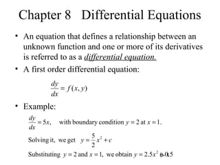
Chapter 8 Differential Equations
• An equation that defines a relationship between an
unknown function and one or more of its derivatives
is referred to as a differential equation.
• A first order differential equation:
• Example:
),( yxf
dx
dy
=
5.05.2obtainwe,1and2ngSubstituti
2
5
getweit,Solving
.1at2conditionboundarywith,5
2
2
−===
+=
===
xyxy
cxy
xyx
dx
dy
2. 8- 2
• Example:
• A second-order differential equation:
• Example:
),,(2
2
dx
dy
yxf
dx
yd
=
)( xyc
dx
dy
−=
'2'' yxyxy ++=
3. 8- 3
Taylor Series Expansion
• Fundamental case, the first-order ordinary differential
equation:
Integrate both sides
• The solution based on Taylor series expansion:
00 atsubject to)( xxyyxf
dx
dy
===
∫∫ =
x
x
y
y
dxxfdy
00
)( ∫+==
x
x
dxxfyxgy
0
)()(or 0
)()('and)(where
...)(''
!2
)(
)(')()()(
0000
0
2
0
00
xfxgxgy
xg
xx
xgxxxgxgy
==
+
−
+−+==
4. 8- 4
Example : First-order Differential
Equation
Given the following differential equation:
The higher-order derivatives:
1at1such that3 2
=== xyx
dx
dy
4nfor0
6
6
3
3
2
2
≥=
=
=
n
n
dx
yd
dx
yd
x
dx
yd
5. 8- 5
The final solution:
1where
)1()1(3)1(31
)6(
!3
)1(
)6(
!2
)1(
)3)(1(1
!3
)1(
!2
)1(
)1(1)(
0
32
3
0
2
2
0
3
33
2
22
=
−+−+−+=
−
+
−
+−+=
−
+
−
+−+=
x
xxx
x
x
x
xx
dx
ydx
dx
ydx
dx
dy
xxg
6. 8- 6
x One Term Two Terms Three Terms Four Terms
1 1 1 1 1
1.1 1 1.3 1.33 1.331
1.2 1 1.6 0.72 1.728
1.3 1 1.9 2.17 2.197
1.4 1 2.2 2.68 2.744
1.5 1 2.5 3.25 3.375
1.6 1 2.8 3.88 4.096
1.7 1 3.1 4.57 4.913
1.8 1 3.4 5.32 5.832
1.9 1 3.7 6.13 6.859
2 1 4 7 8
Table: Taylor Series Solution
8. 8- 8
General Case
• The general form of the first-order ordinary
differential equation:
• The solution based on Taylor series expansion:
00 atsubject to),( xxyyyxf
dx
dy
===
...),(''
!2
)(
),(')(),()( 00
0
00000 +
−
+−+== yxg
xx
yxgxxyxgxgy
9. 8- 9
Euler’s Method
• Only the term with the first derivative is used:
• This method is sometimes referred to as the one-step
Euler’s method, since it is performed one step at a
time.
e
dx
dy
xxxgxg +−+= )()()( 00
10. 8- 10
Example: One-step Euler’s Method
• Consider the differential equation:
• For x =1.1
Therefore, at x=1.1, y=1.44133 (true value).
1at1such that4 2
=== xyx
dx
dy
∫∫ =
1.1
1
2
1
4 dxxdy
y
44133.0
3
4
1
1.1
1
3
==− xy
12. 8- 12
Errors with Euler`s Method
• Local error: over one step size.
Global error: cumulative over the range of the solution.
• The error ε using Euler`s method can be approximated using the
second term of the Taylor series expansion as
• If the range is divided into n increments, then the error at the end
of range for x would be nε.
].,[inmaximumtheiswhere
!2
)(
02
2
2
22
0
xx
dx
yd
dx
ydxx −
=ε
18. 8- 18
Modified Euler’s Method
• Use an average slope, rather than the slope at the start
of the interval :
a. Evaluate the slope at the start of the interval
b. Estimate the value of the dependent variable y at the
end of the interval using the Euler’s metod.
c. Evaluate the slope at the end of the interval.
d. Find the average slope using the slopes in a and c.
e. Compute a revised value of the dependent variable y
at the end of the interval using the average slope of
step d with Euler’s method.
19. 8- 19
Example : Modified Euler’s Method
1at1thatsuch === xyyx
dx
dy
10768.1)07684.1(1.01)0.11.1()0.1()1.1(1e.
07684.1)15369.11(
2
1
1d.
15369.11.11.1c.1
1.1)1(1.01)0.11.1()0.1()1.1(1b.
111a.1
:1.0foriterationfirsttheofstepsfiveThe
1.1
1
1
=+=−+=
=+=
==
=+=−+=
==
=∆
a
a
dx
dy
gg
dx
dy
dx
dy
dx
dy
gg
dx
dy
x
21. 8- 21
Second-order Runge-Kutta Methods
• The modified Euler’s method is a case of the second-
order Runge-Kutta methods. It can be expressed as
xhxxx
xxgyxgy
hyxhfyhxfyxfyy
ii
iiii
iiiiiiii
∆=∆+=
∆+==
++++=
+
+
+
,
),(),(where
))],(,(),([5.0
1
1
1
22. 8- 22
• The computations according to Euler’s method:
1. Evaluate the slope at the start of an interval, that is,
at (xi,yi) .
2. Evaluate the slope at the end of the interval (xi+1,yi+1) :
3. Evaluate yi+1 using the average slope S1 of and S2 :
),(1 ii yxfS =
),( 12 hSyhxfS ii ++=
hSSyy ii )(5.0 211 ++=+
23. 8- 23
Third-order Runge-Kutta Methods
• The following is an example of the third-order Runge-
Kutta methods :
hyxhfyhxhfyxhfyhxf
yxhfyhxfyxfyy
iiiiiiii
iiiiiiii
)))],(5.0,5.0(2),(,(
)),(5.0,5.0(4),([
6
1
1
+++−+
+++++=+
24. 8- 24
• The computational steps for the third-order method:
1. Evaluate the slope at (xi,yi).
2. Evaluate a second slope S2 estimate at the mid-point
in of the step as
3. Evaluate a third slope S3 as
4. Estimate the quantity of interest yi+1 as
)5.0,5.0( 12 hSyhxfS ii ++=
)2,( 213 hShSyhxfS ii +−+=
hSSSyy ii ]4[
6
1
3211 +++=+
),(1 ii yxfS =
25. 8- 25
Fourth-order Runge-Kutta Methods
1. Compute the slope S1 at (xi,yi).
2. Estimate y at the mid-point of the interval.
3. Estimate the slope S2 at mid-interval.
4. Revise the estimate of y at mid-interval
.atthatsuch),( 00 hxxxyyyxf
dx
dy
=∆===
),(1 ii yxfS =
),(
2
2/1 iiii yxf
h
yy +=+
)5.0,5.0( 12 hSyhxfS ii ++=
22/1
2
S
h
yy ii +=+
26. 8- 26
5. Compute a revised estimate of the slope S3 at mid-
interval.
6. Estimate y at the end of the interval.
7. Estimate the slope S4 at the end of the interval
8. Estimate yi+1 again.
)5.0,5.0( 23 hSyhxfS ii ++=
31 hSyy ii +=+
),( 34 hSyhxfS ii ++=
)22(
6
43211 SSSS
h
yy ii ++++=+
27. 8- 27
Predictor-Corrector Methods
• Unless the step sizes are small, Euler’s method
and Runge-Kutta may not yield precise
solutions.
• The Predictor-Corrector Methods iterate
several times over the same interval until the
solution converges to within an acceptable
tolerance.
• Two parts: predictor part and corrector part.
28. 8- 28
Euler-trapezoidal Method
• Euler’s method is the predictor algorithm.
• The trapezoidal rule is the corrector equation.
• Eluer formula (predictor):
• Trapezoidal rule (corrector):
The corrector equation can be applied as many times as
necessary to get convergence.
,*
,*,1
i
iji
dx
dy
hyy +=+
][
2 1,1,*
,*,1
−+
+ ++=
jii
iji
dx
dy
dx
dyh
yy
29. 8- 29
Example 8-6: Euler-trapezoidal Mehtod
1at1thatsuch:Problem === xyyx
dx
dy
1.1)1(1.01
1.0
111
is1.1atforestimate)(predictorinitialThe
0,1
0,0
,*00,1
0,0
=+=
+=
==
=
y
dx
dy
yy
dx
dy
xy
15369.11.11.1
:estimatetheimprovetousedisequationcorrectorThe
0,1
==
dx
dy
33. 8- 33
Milne-Simpson Method
• Milne’s equation is the predictor euqation.
• The Simpson’s rule is the corrector formula.
• Milne’s equation (predictor):
For the two initial sampling points, a one-step
method such as Euler’s equation can be used.
• Simpsos’s rule (corrector):
]22[
3
4
,*2,*1,*
,*30,1
−−
−+ +−+=
iii
ii
dx
dy
dx
dy
dx
dyh
yy
]4[
3 ,*1,*,1
,*1,1
−+
−+ +++=
iiji
iji
dx
dy
dx
dy
dx
dyh
yy
34. 8- 34
Example 8-7: Milne-Simpson Mehtod
.4.1and3.1atestimatewant toWe
1at1thatsuch:Problem
==
===
xxy
xyyx
dx
dy
1 1 1
1.1 1.10789 1.15782
1.2 1.23239 1.33215
Assume that we have the following values,
obtained from the Euler-trapezoidal method
in Example 8-6.
x y dx
dy
39. 8- 39
Least-Squares Method
• The procedure for deriving the least-squares
function:
1. Assume the solution is an nth-order polynomial:
2. Use the boundary condition of the ordinary
differential equation to evaluate one of (bo,b1,b2,
…,bn).
3. Define the objective function:
n
nx xbxbbby ++++= 2
210ˆ
dxeF
x∫= 2
dx
dy
dx
yd
e −=
ˆ
where
40. 8- 40
4. Find the minimum of F with respect to the unknowns
(b1,b2, b3,…,bn) , that is
5. The integrals in Step 4 are called the normal
equations; the solution of the normal equations yields
value of the unknowns (b1,b2, b3,…,bn).
∫ =
∂
∂
=
∂
∂
xall
ii
dx
b
e
e
b
F
02
41. 8- 41
Example 8-8: Least-squares Method
2/2
:solutionAnalytical
1.x0intervalfor theitSolve
0at1thatsuch:Problem
x
ey
xyxy
dx
dy
=
≤≤
===
1
1
0
10
10
ˆ
1ˆ
ismodellineartheThus.1yields
)0(1ˆ
conditionboundarytheUsing
ˆ
b
dx
yd
xby
b
bby
xbby
=
+=
=
+==
+=
• First, assume a linear model is used:
43. 8- 43
x True y Value Numerical y Value Error (%)
0 1. 1. -
0.2 1.0202 1.0938 7.2
0.4 1.0833 1.1875 9.6
0.6 1.1972 1.2812 7.0
0.8 1.3771 1.3750 0.0
1.0 1.6487 1.46688 -10.9
Table: A linear model for the least-squares method
2/2
x
ey = xy 32
15
1ˆ +=
44. 8- 44
• Next, to improve the accuracy of estimates, a
quadratic model is used:
xxxbxb
xbxbxxbbxyxbbe
xbb
dx
yd
b
bbby
xbxbby
−−+−=
++−+=−+=
+=
=
++==
++=
)2()1(
)1(22
isfunctionerrorThe
2
ˆ
.1yields
)0()0(1ˆ
conditionboundarytheUsing
ˆ
3
2
2
1
2
212121
21
0
2
210
2
210
47. 8- 47
x True y Value Numerical y Value Error (%)
0 1. 1. -
0.2 1.0202 1.0022 -1.8
0.4 1.0833 1.0674 0.0
0.6 1.1972 1.1956 0.0
0.8 1.3771 1.38668 0.0
1.0 1.6487 1.6411 0.0
Table: A quadratic model for the least-squares method
2/2
x
ey = 2
78776.014669.01ˆ xxy +−=
48. 8- 48
Galerkin Method
• Example: Galerkin Method
The same problem as Example 8-8.
Use the quadratic approximating equation.
i
i
i
x
i
b
e
w
w
niedxw
∂
∂
=
==∫
method,squaresleastFor the
factor.nga weightiiswhere
...2,10
.andLet 2
21 xwxw ==
50. 8- 50
Table: Example for the Galerkin method
x True y value Numerical y value Error
(%)
0 1. 1. --
0.2 1.0202 0.9816 0.0
0.4 1.0833 1.0316 0.0
0.6 1.1972 1.1500 0.0
0.8 1.3771 1.3368 0.0
1.0 1.6487 1.5921 0.0
2/2
x
ey = 2
85526.026316.01ˆ xxy +−=
51. 8- 51
Higher-Order Differential Equations
• Second order differential equation:
Transform it into a system of first-order differential
equations.
dx
dy
dx
dy
yyy
y
dx
dy
yyxf
dx
dy
===
=
=
1
21
2
1
21
2
andwhere
),,(
=
dx
dy
yxf
dx
yd
,,2
2
52. 8- 52
• In general, any system of n equations of the following
type can be solved using any of the previously
discussed methods:
),...,,(
),...,,(
),...,,(
),...,,(
21
213
3
212
2
211
1
nn
n
n
n
n
yyyxf
dx
dy
yyyxf
dx
dy
yyyxf
dx
dy
yyyxf
dx
dy
=
=
=
=
53. 8- 53
Example: Second-order Differential Equation
EI
XX
EI
M
dX
Yd 2
2
2
10
:Problem
−
==
Z
dX
dY
EI
XX
EI
M
dX
dZ
=
−
==
10
:intomedtransforbecanIt
2
hZYXfYY
hZYXfZZ
ZYXEI
iiiii
iiiii
),,(
),,(
:equationsfollowingthesolvetomethodsEuler'Use
02314.0and0,0at3600Assume
11
21
+=
+=
−====
+
+
54. 8- 54
Table: Second-order Differential Equation
Using a Step Size of 0.1 Ft
X
(ft)
Y
(ft)
Exact Z Exact Y
(ft)
0 0 -0.0231481 0 -0.0231481 0
0.1 0.000275 -0.0231481 -0.0023148 -0.0231344 -0.0023144
0.2 0.0005444 -0.0231206 -0.0046296 -0.0230933 -0.004626
0.3 0.0008083 -0.0230662 -0.0069417 -0.0230256 -0.0069321
0.4 0.0010667 -0.0229854 -0.0092483 -0.0229319 -0.0092302
0.5 0.0013194 -0.0228787 -0.0115469 -0.0228125 -0.0115177
0.6 0.0015667 -0.0227468 -0.0138347 -0.0226681 -0.0137919
0.7 0.0018083 -0.0225901 -0.0161094 -0.0224994 -0.0160505
0.8 0.0020444 -0.0224093 -0.0183684 -0.0223067 -0.018291
0.9 0.002275 -0.0222048 -0.0206093 -0.0220906 -0.020511
dX
dZ
dX
dY
Z =
55. 8- 55
Table: Second-order Differential Equation
Using a Step Size of 0.1 Ft (continued)
dX
dZ
dX
dY
Z =
X
(ft)
Y
(ft)
Exact Z Exact Y
(ft)
1 0.0025 -0.0219773 -0.0228298 -0.0218519 -0.0227083
2 0.0044444 -0.0185565 -0.0434305 -0.0183333 -0.04296663
3 0.0058333 -0.0134412 -0.0298019 -0.0131481 -0.0588194
4 0.0066667 -0.007187 -0.0704998 -0.0068519 -0.0688889
5 0.0069444 -0.0003495 -0.0746352 0.00000000 -0.071228
6 0.0066667 0.0065157 -0.0718747 0.0068519 -0.0688889
7 0.0058333 0.0128532 -0.06244066 0.0131481 -0.0588194
8 0.0044444 0.0181074 -0.0471107 0.0183333 -0.042963
9 0.0025 0.0217227 -0.0272183 0.0278519 -0.0227083
10 0.000000 0.0231435 -0.00466523 0.0231481 0.000000