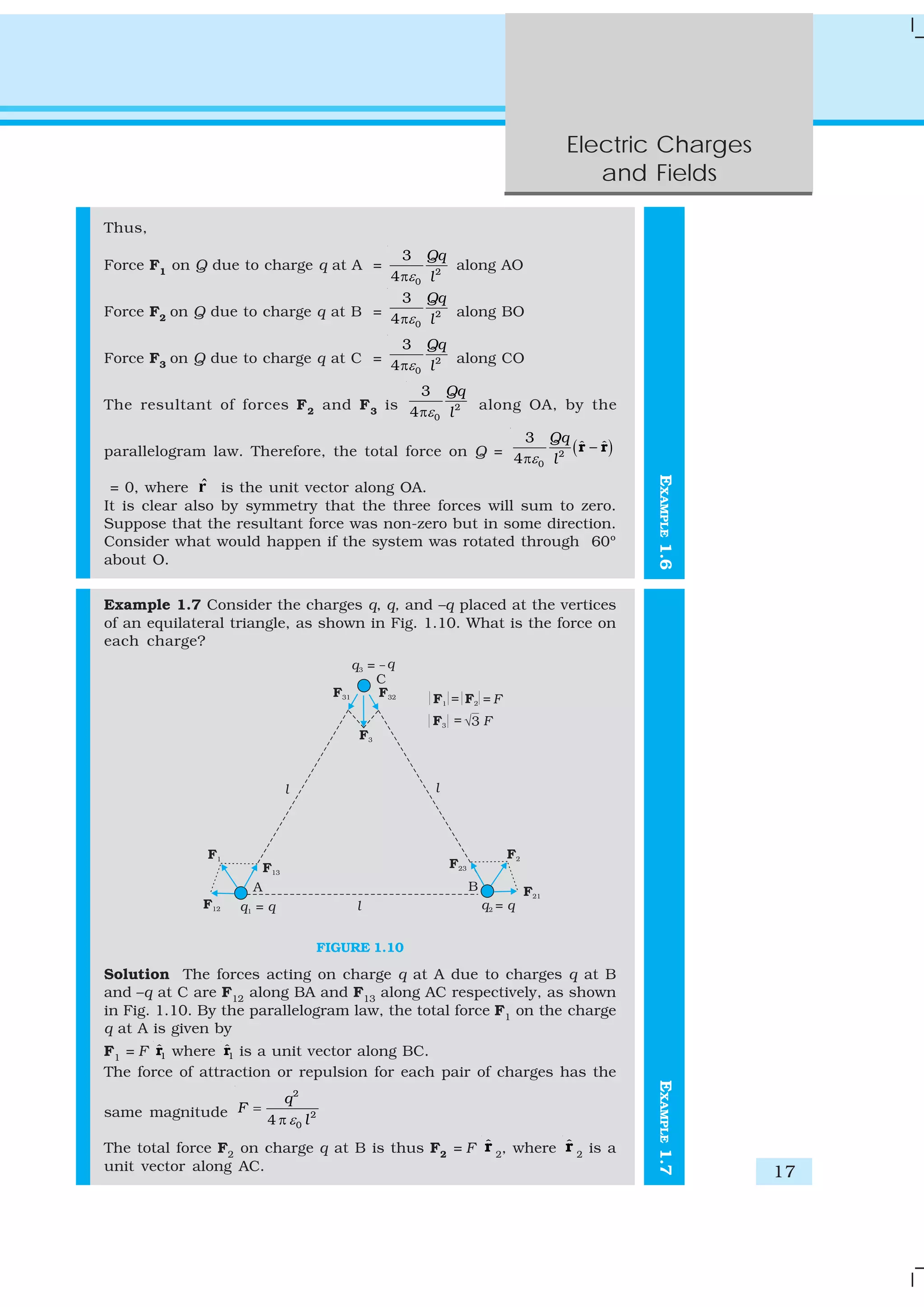
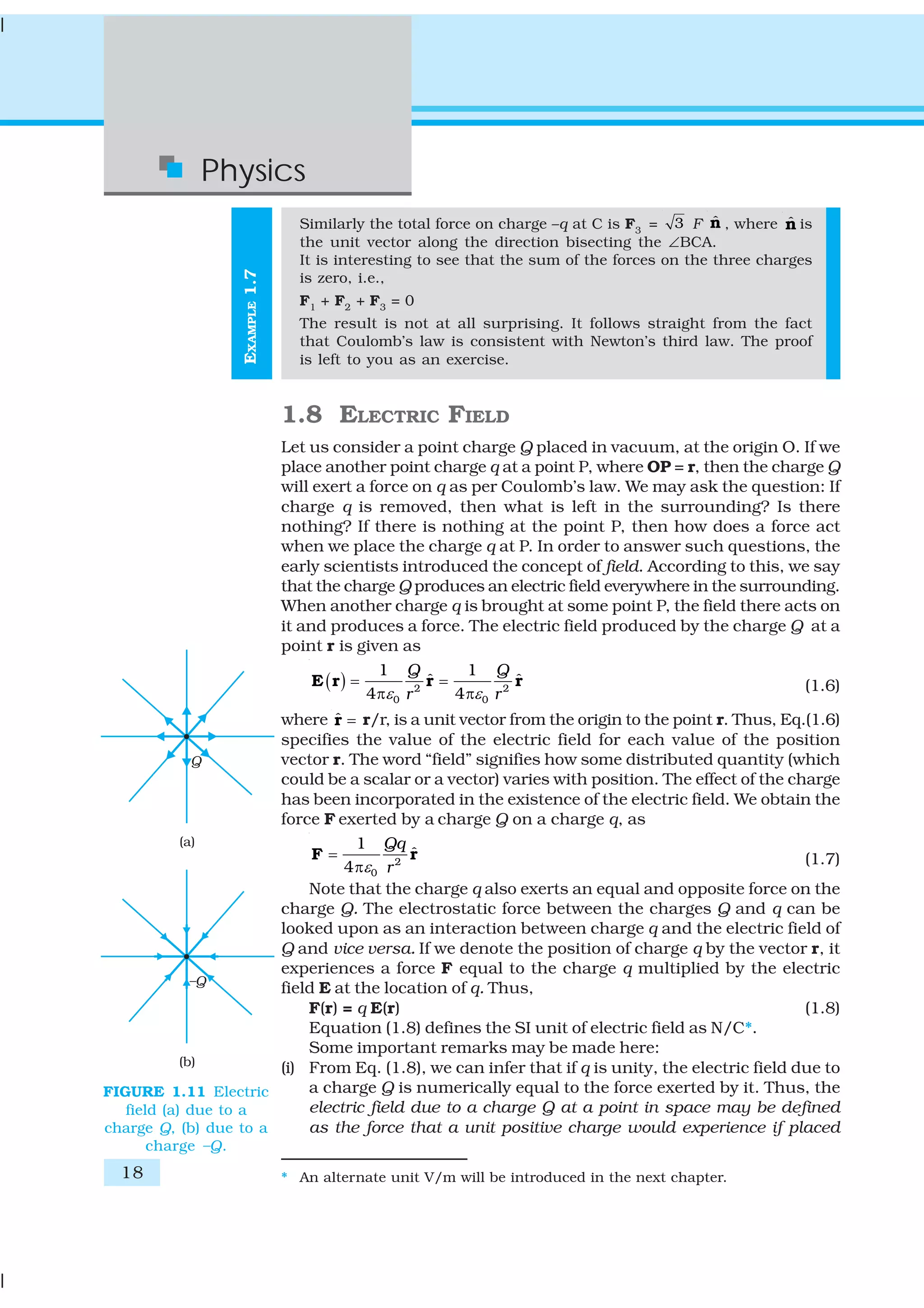
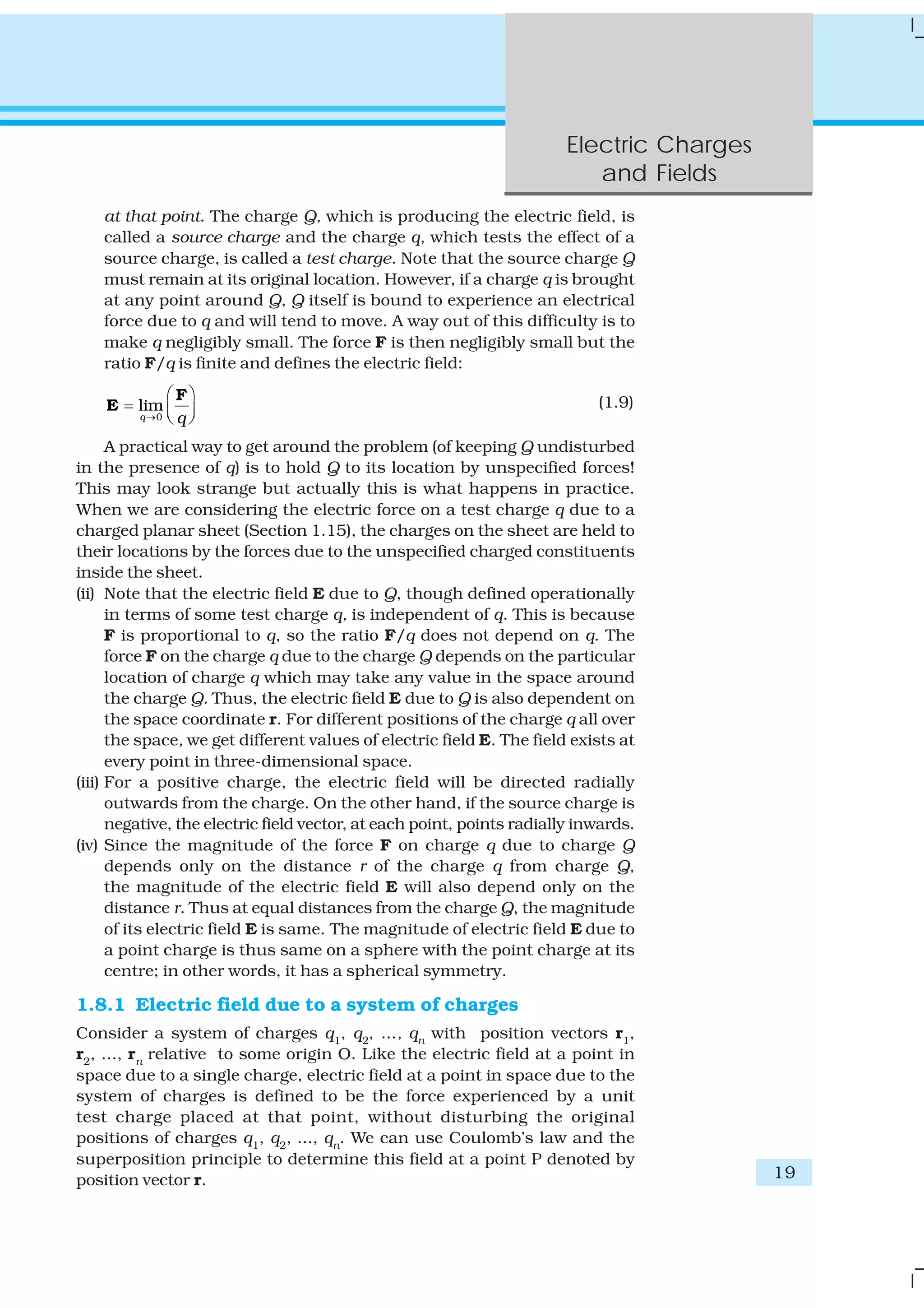
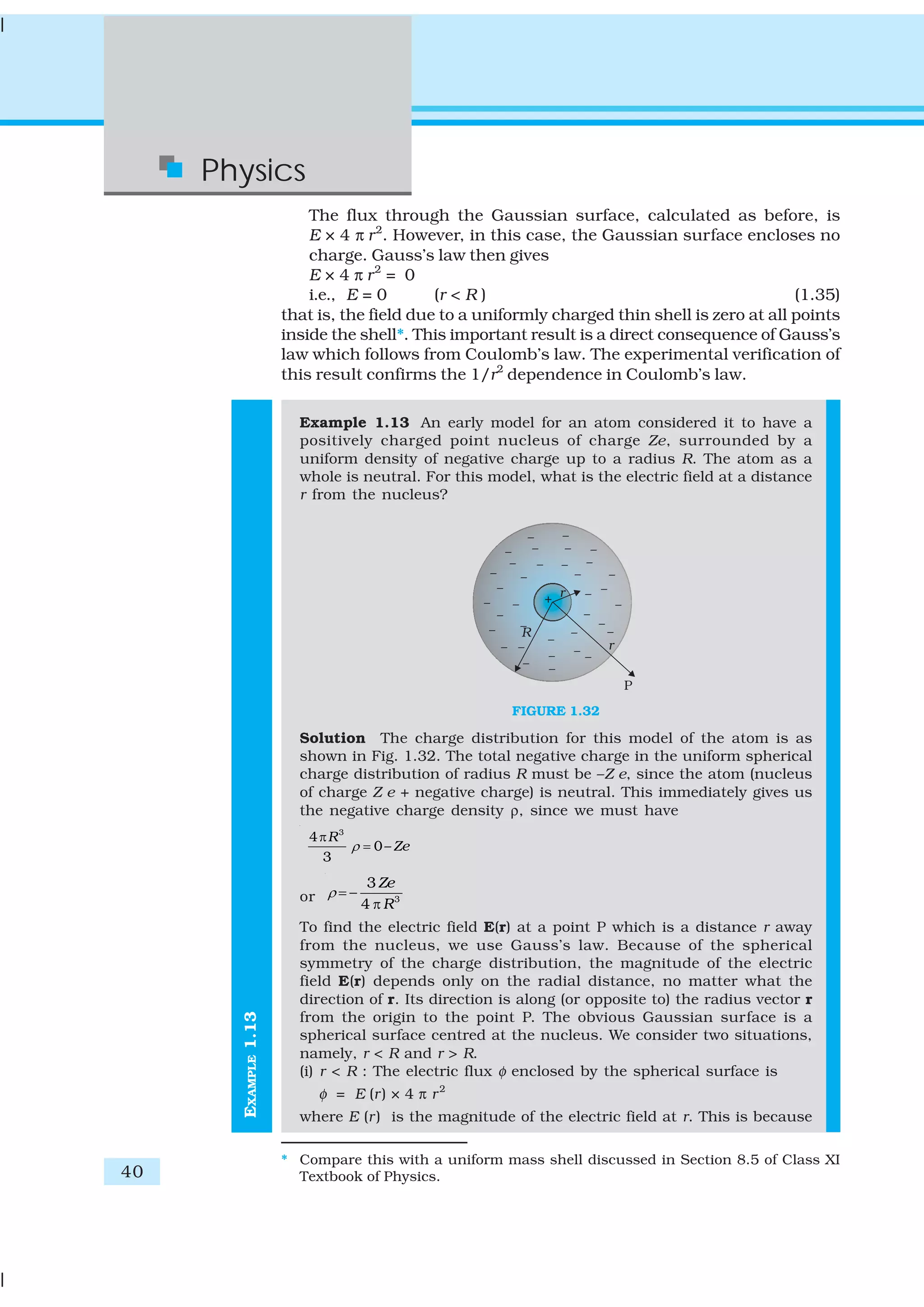
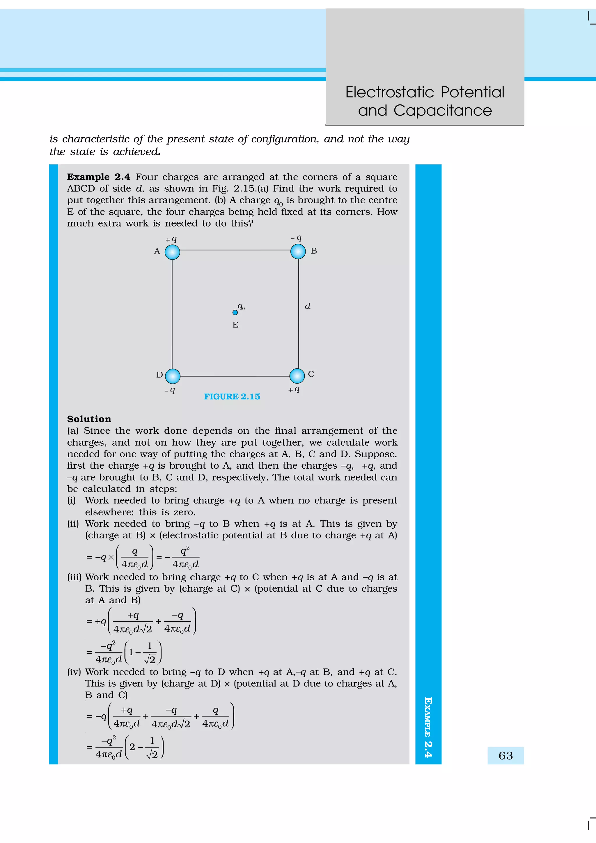
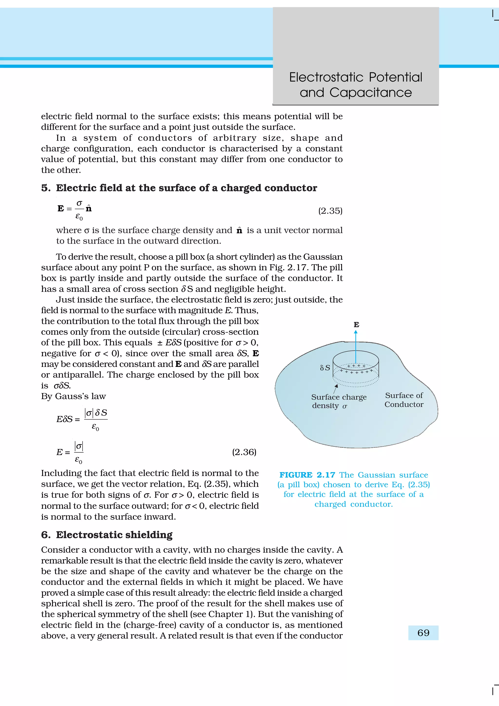
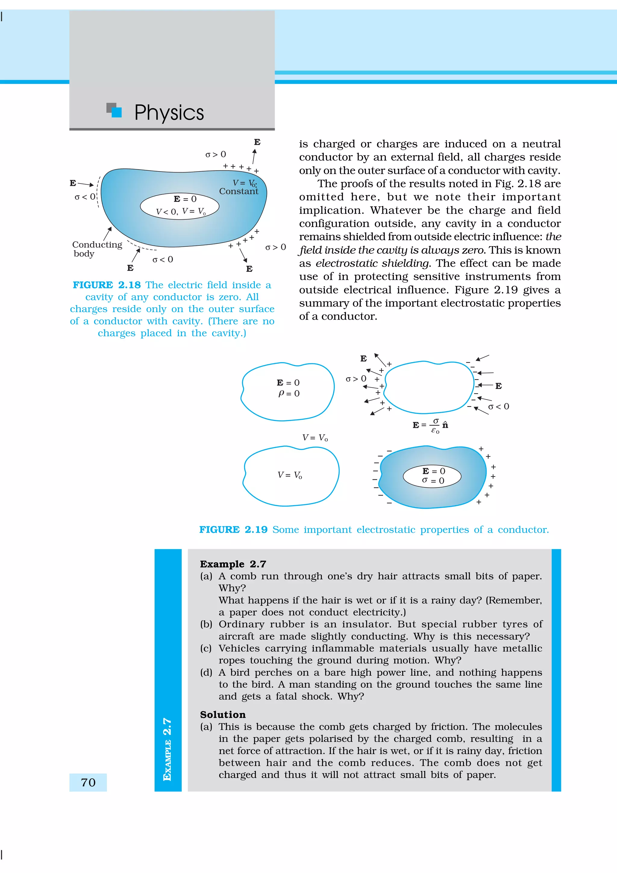
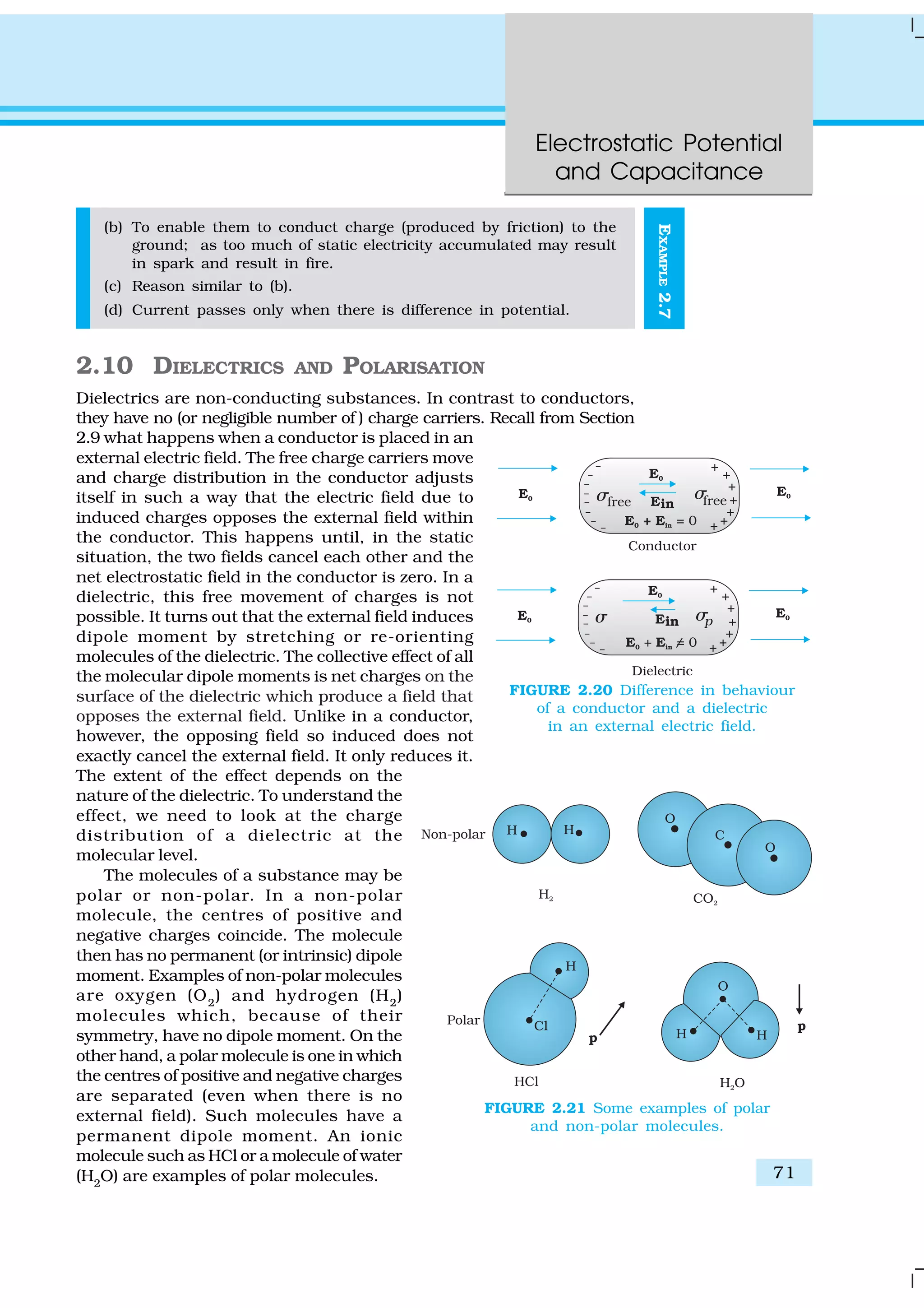
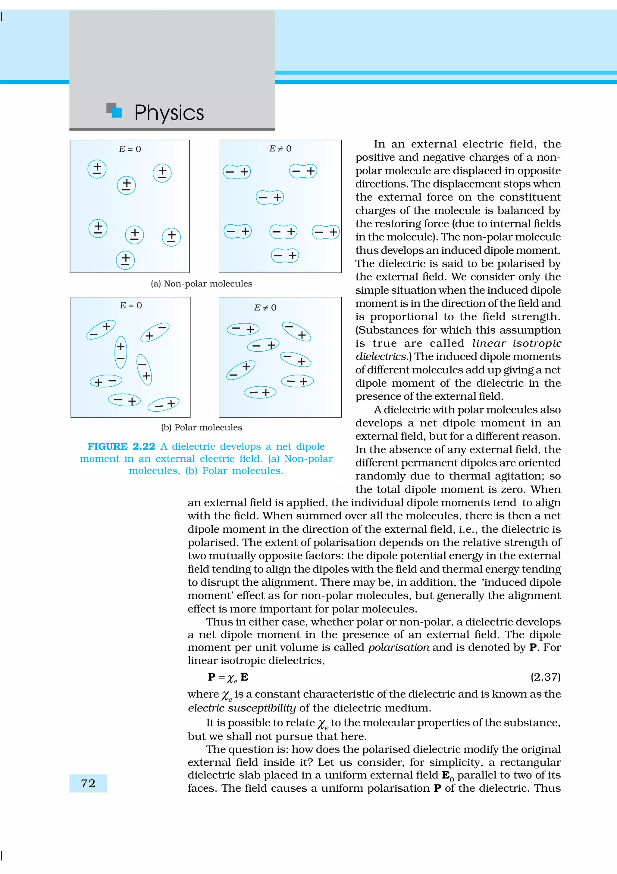
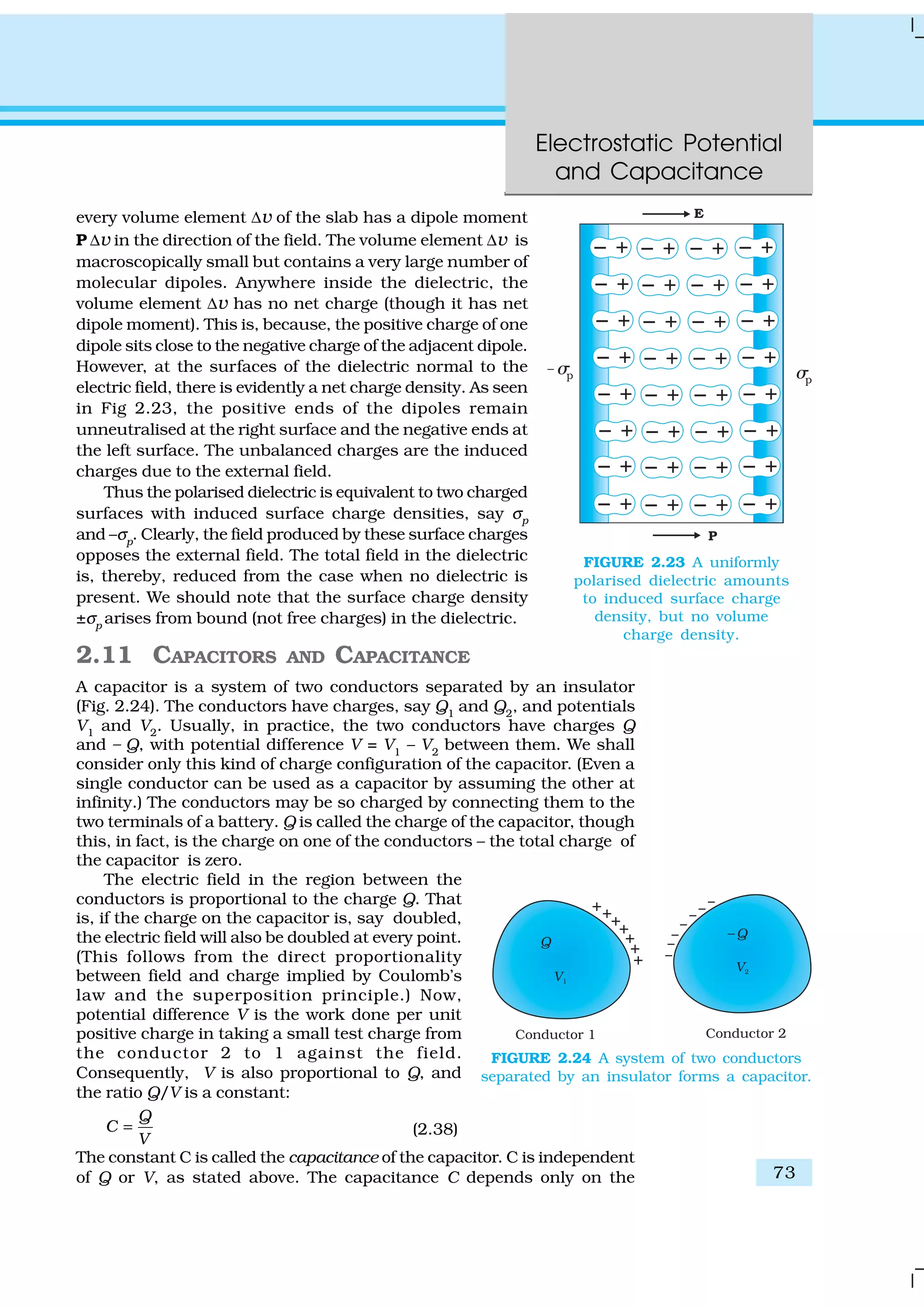
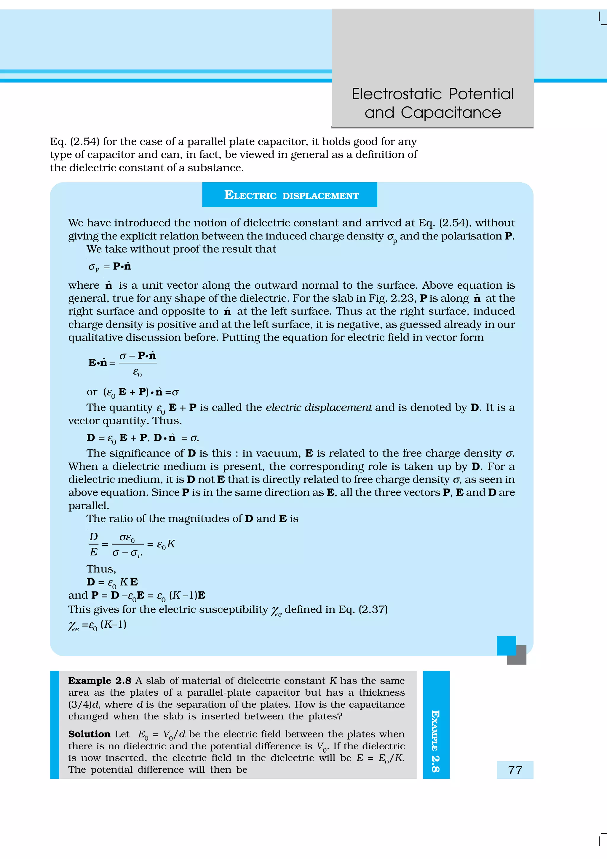
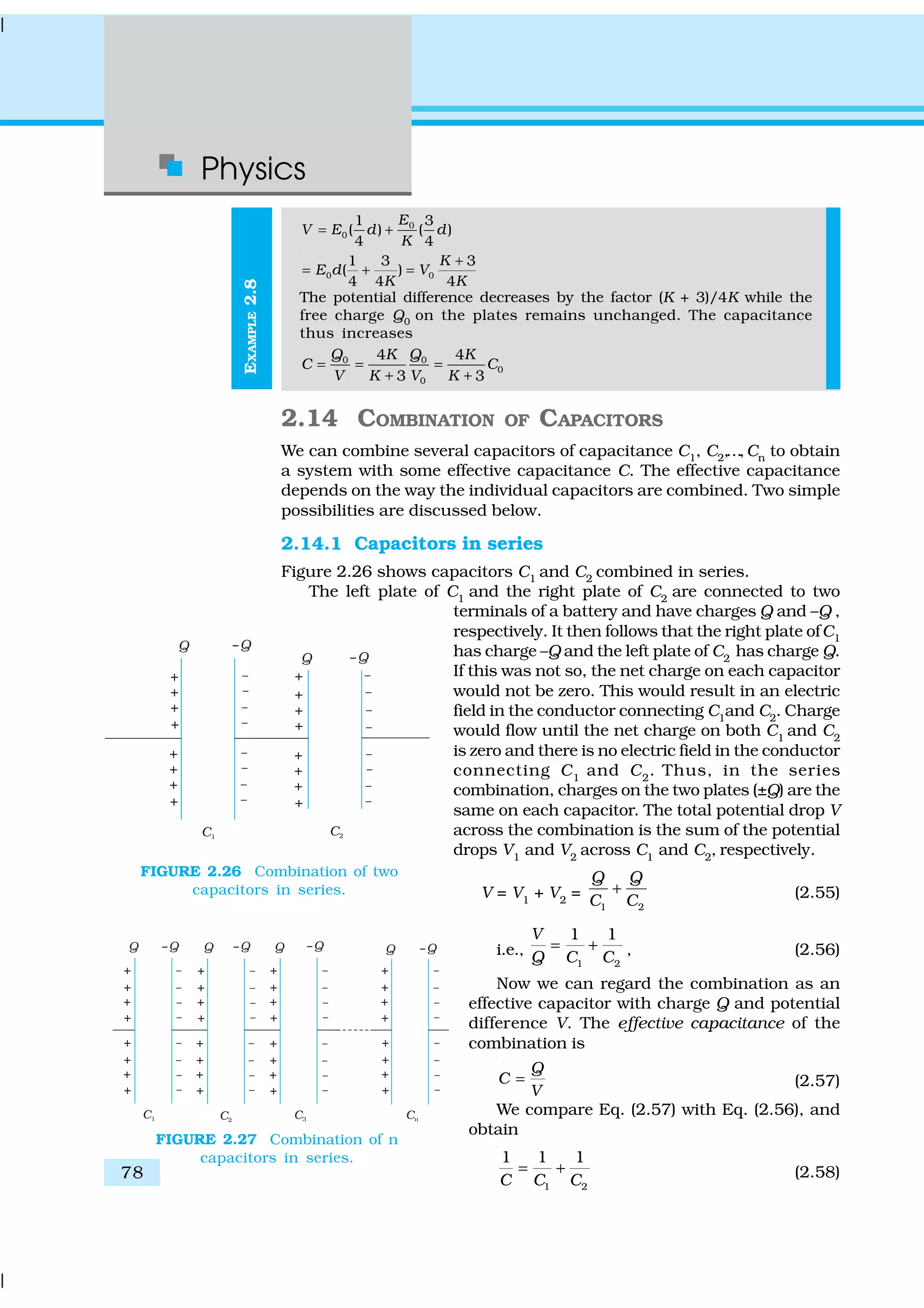
This document is the first chapter of a physics textbook on electric charges and fields. It introduces the topic of electrostatics and discusses how objects can acquire electric charges through rubbing. It describes early experiments showing that there are two types of charges (positive and negative) which attract if opposite but repel if like. Conductors and insulators are introduced, with conductors able to distribute charge easily over their surface. The chapter establishes the basics of electric charge and sets up further discussion of electric fields and forces.

1. -
I

2. CONTENTS
FOREWORD v
PREFACE xi
CHAPTER ONE
ELECTRIC CHARGES AND FIELDS
1.1 Introduction 1
1.2 Electric Charges 1
1.3 Conductors and Insulators 5
1.4 Charging by Induction 6
1.5 Basic Properties of Electric Charge 8
1.6 Coulomb’s Law 10
1.7 Forces between Multiple Charges 15
1.8 Electric Field 18
1.9 Electric Field Lines 23
1.10 Electric Flux 25
1.11 Electric Dipole 27
1.12 Dipole in a Uniform External Field 31
1.13 Continuous Charge Distribution 32
1.14 Gauss’s Law 33
1.15 Application of Gauss’s Law 37
CHAPTER TWO
ELECTROSTATIC POTENTIAL AND CAPACITANCE
2.1 Introduction 51
2.2 Electrostatic Potential 53
2.3 Potential due to a Point Charge 54
2.4 Potential due to an Electric Dipole 55
2.5 Potential due to a System of Charges 57
2.6 Equipotential Surfaces 60
2.7 Potential Energy of a System of Charges 61
2.8 Potential Energy in an External Field 64
2.9 Electrostatics of Conductors 67
2.10 Dielectrics and Polarisation 71
2.11 Capacitors and Capacitance 73
2.12 The Parallel Plate Capacitor 74
2.13 Effect of Dielectric on Capacitance 75

3. 2.14 Combination of Capacitors 78
2.15 Energy Stored in a Capacitor 80
2.16 Van de Graaff Generator 83
CHAPTER THREE
CURRENT ELECTRICITY
3.1 Introduction 93
3.2 Electric Current 93
3.3 Electric Currents in Conductors 94
3.4 Ohm’s law 95
3.5 Drift of Electrons and the Origin of Resistivity 97
3.6 Limitations of Ohm’s Law 101
3.7 Resistivity of various Materials 101
3.8 Temperature Dependence of Resistivity 103
3.9 Electrical Energy, Power 105
3.10 Combination of Resistors — Series and Parallel 107
3.11 Cells, emf, Internal Resistance 110
3.12 Cells in Series and in Parallel 113
3.13 Kirchhoff’s Laws 115
3.14 Wheatstone Bridge 118
3.15 Meter Bridge 120
3.16 Potentiometer 122
CHAPTER FOUR
MOVING CHARGES AND MAGNETISM
4.1 Introduction 132
4.2 Magnetic Force 133
4.3 Motion in a Magnetic Field 137
4.4 Motion in Combined Electric and Magnetic Fields 140
4.5 Magnetic Field due to a Current Element, Biot-Savart Law 143
4.6 Magnetic Field on the Axis of a Circular Current Loop 145
4.7 Ampere’s Circuital Law 147
4.8 The Solenoid and the Toroid 150
4.9 Force between Two Parallel Currents, the Ampere 154
4.10 Torque on Current Loop, Magnetic Dipole 157
4.11 The Moving Coil Galvanometer 163
CHAPTER FIVE
MAGNETISM AND MATTER
5.1 Introduction 173
5.2 The Bar Magnet 174
xiv

4. 5.3 Magnetism and Gauss’s Law 181
5.4 The Earth’s Magnetism 185
5.5 Magnetisation and Magnetic Intensity 189
5.6 Magnetic Properties of Materials 191
5.7 Permanent Magnets and Electromagnets 195
CHAPTER SIX
ELECTROMAGNETIC INDUCTION
6.1 Introduction 204
6.2 The Experiments of Faraday and Henry 205
6.3 Magnetic Flux 206
6.4 Faraday’s Law of Induction 207
6.5 Lenz’s Law and Conservation of Energy 210
6.6 Motional Electromotive Force 212
6.7 Energy Consideration: A Quantitative Study 215
6.8 Eddy Currents 218
6.9 Inductance 219
6.10 AC Generator 224
CHAPTER SEVEN
ALTERNATING CURRENT
7.1 Introduction 233
7.2 AC Voltage Applied to a Resistor 234
7.3 Representation of AC Current and Voltage by
Rotating Vectors — Phasors 237
7.4 AC Voltage Applied to an Inductor 237
7.5 AC Voltage Applied to a Capacitor 241
7.6 AC Voltage Applied to a Series LCR Circuit 244
7.7 Power in AC Circuit: The Power Factor 252
7.8 LC Oscillations 255
7.9 Transformers 259
CHAPTER EIGHT
ELECTROMAGNETIC WAVES
8.1 Introduction 269
8.2 Displacement Current 270
8.3 Electromagnetic Waves 274
8.4 Electromagnetic Spectrum 280
ANSWERS 288
xv

5. 1.1 INTRODUCTION
All of us have the experience of seeing a spark or hearing a crackle when
we take off our synthetic clothes or sweater, particularly in dry weather.
This is almost inevitable with ladies garments like a polyester saree. Have
you ever tried to find any explanation for this phenomenon? Another
common example of electric discharge is the lightning that we see in the
sky during thunderstorms. We also experience a sensation of an electric
shock either while opening the door of a car or holding the iron bar of a
bus after sliding from our seat. The reason for these experiences is
discharge of electric charges through our body, which were accumulated
due to rubbing of insulating surfaces. You might have also heard that
this is due to generation of static electricity. This is precisely the topic we
are going to discuss in this and the next chapter. Static means anything
that does not move or change with time. Electrostatics deals with the
study of forces, fields and potentials arising from static charges.
1.2 ELECTRIC CHARGE
Historically the credit of discovery of the fact that amber rubbed with
wool or silk cloth attracts light objects goes to Thales of Miletus, Greece,
around 600 BC. The name electricity is coined from the Greek word
elektron meaning amber. Many such pairs of materials were known which
Chapter One
ELECTRIC CHARGES
AND FIELDS

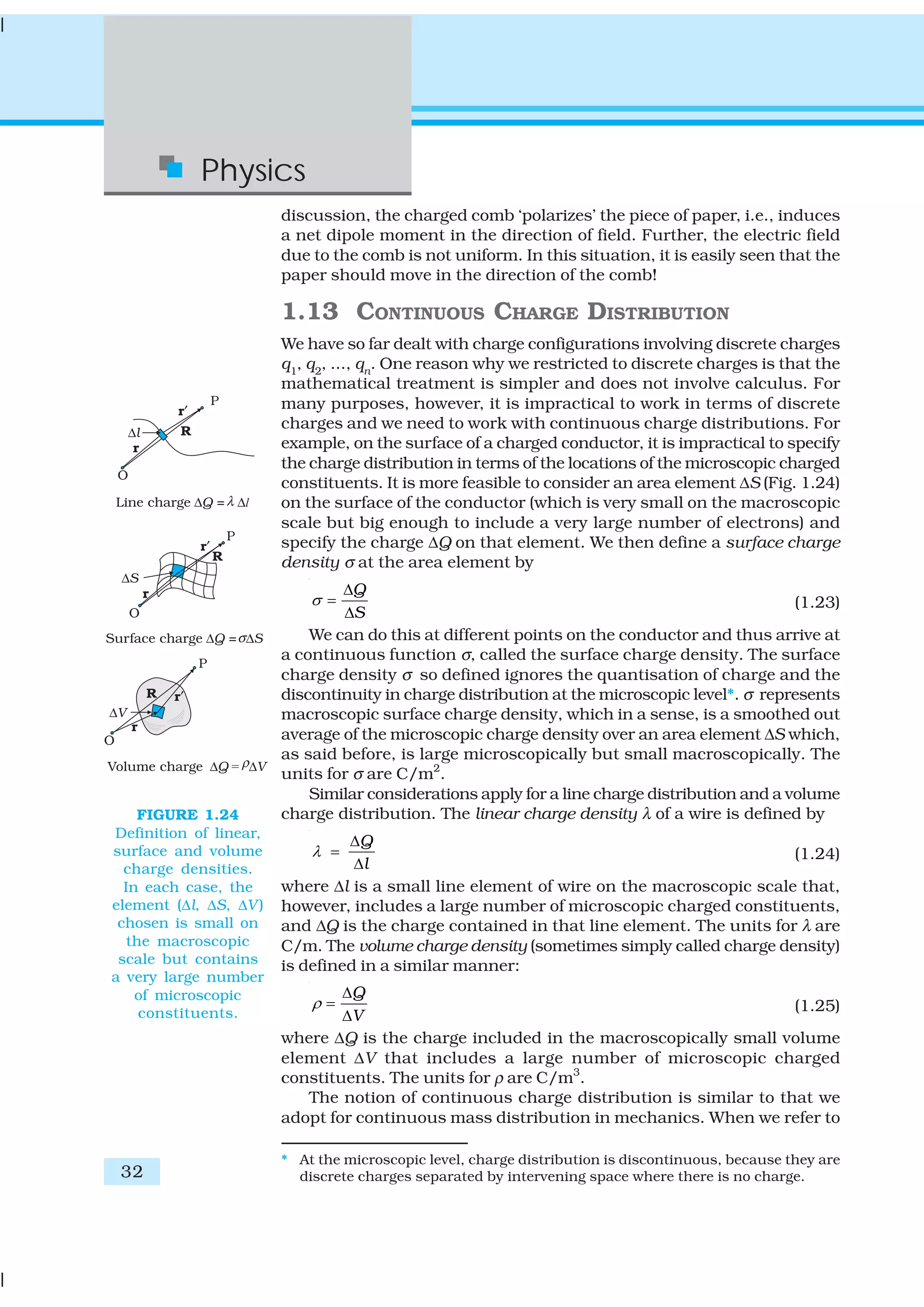
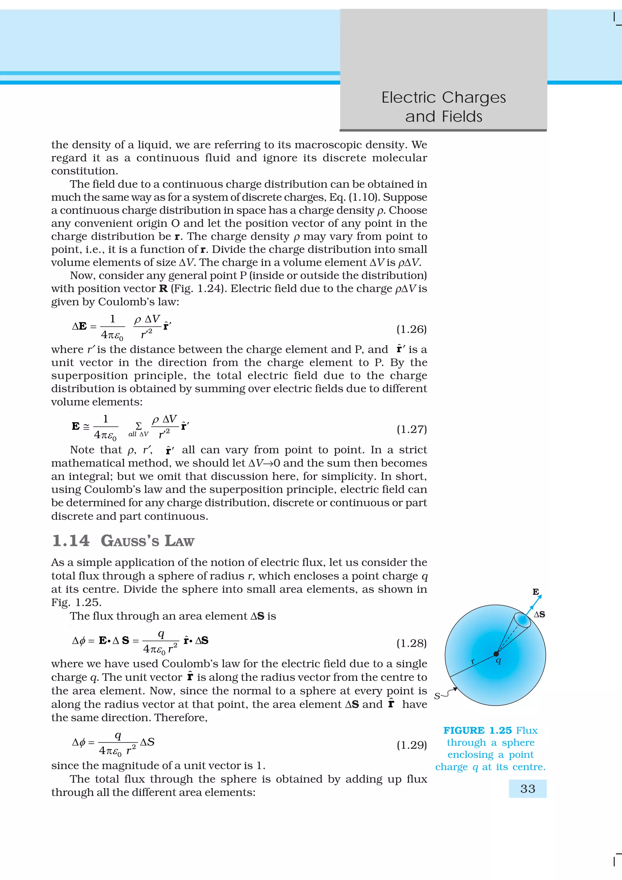
6. 2
Physics
on rubbing could attract light objects
like straw, pith balls and bits of papers.
You can perform the following activity
at home to experience such an effect.
Cut out long thin strips of white paper
and lightly iron them. Take them near a
TV screen or computer monitor. You will
see that the strips get attracted to the
screen. In fact they remain stuck to the
screen for a while.
It was observed that if two glass rods
rubbed with wool or silk cloth are
brought close to each other, they repel
each other [Fig. 1.1(a)]. The two strands
of wool or two pieces of silk cloth, with
which the rods were rubbed, also repel
each other. However, the glass rod and
wool attracted each other. Similarly, two plastic rods rubbed with cat’s
fur repelled each other [Fig. 1.1(b)] but attracted the fur. On the other
hand, the plastic rod attracts the glass rod [Fig. 1.1(c)] and repel the silk
or wool with which the glass rod is rubbed. The glass rod repels the fur.
If a plastic rod rubbed with fur is made to touch two small pith balls
(now-a-days we can use polystyrene balls) suspended by silk or nylon
thread, then the balls repel each other [Fig. 1.1(d)] and are also repelled
by the rod. A similar effect is found if the pith balls are touched with a
glass rod rubbed with silk [Fig. 1.1(e)]. A dramatic observation is that a
pith ball touched with glass rod attracts another pith ball touched with
plastic rod [Fig. 1.1(f )].
These seemingly simple facts were established from years of efforts
and careful experiments and their analyses. It was concluded, after many
careful studies by different scientists, that there were only two kinds of
an entity which is called the electric charge. We say that the bodies like
glass or plastic rods, silk, fur and pith balls are electrified. They acquire
an electric charge on rubbing. The experiments on pith balls suggested
that there are two kinds of electrification and we find that (i) like charges
repel and (ii) unlike charges attract each other. The experiments also
demonstrated that the charges are transferred from the rods to the pith
balls on contact. It is said that the pith balls are electrified or are charged
by contact. The property which differentiates the two kinds of charges is
called the polarity of charge.
When a glass rod is rubbed with silk, the rod acquires one kind of
charge and the silk acquires the second kind of charge. This is true for
any pair of objects that are rubbed to be electrified. Now if the electrified
glass rod is brought in contact with silk, with which it was rubbed, they
no longer attract each other. They also do not attract or repel other light
objects as they did on being electrified.
Thus, the charges acquired after rubbing are lost when the charged
bodies are brought in contact. What can you conclude from these
observations? It just tells us that unlike charges acquired by the objects
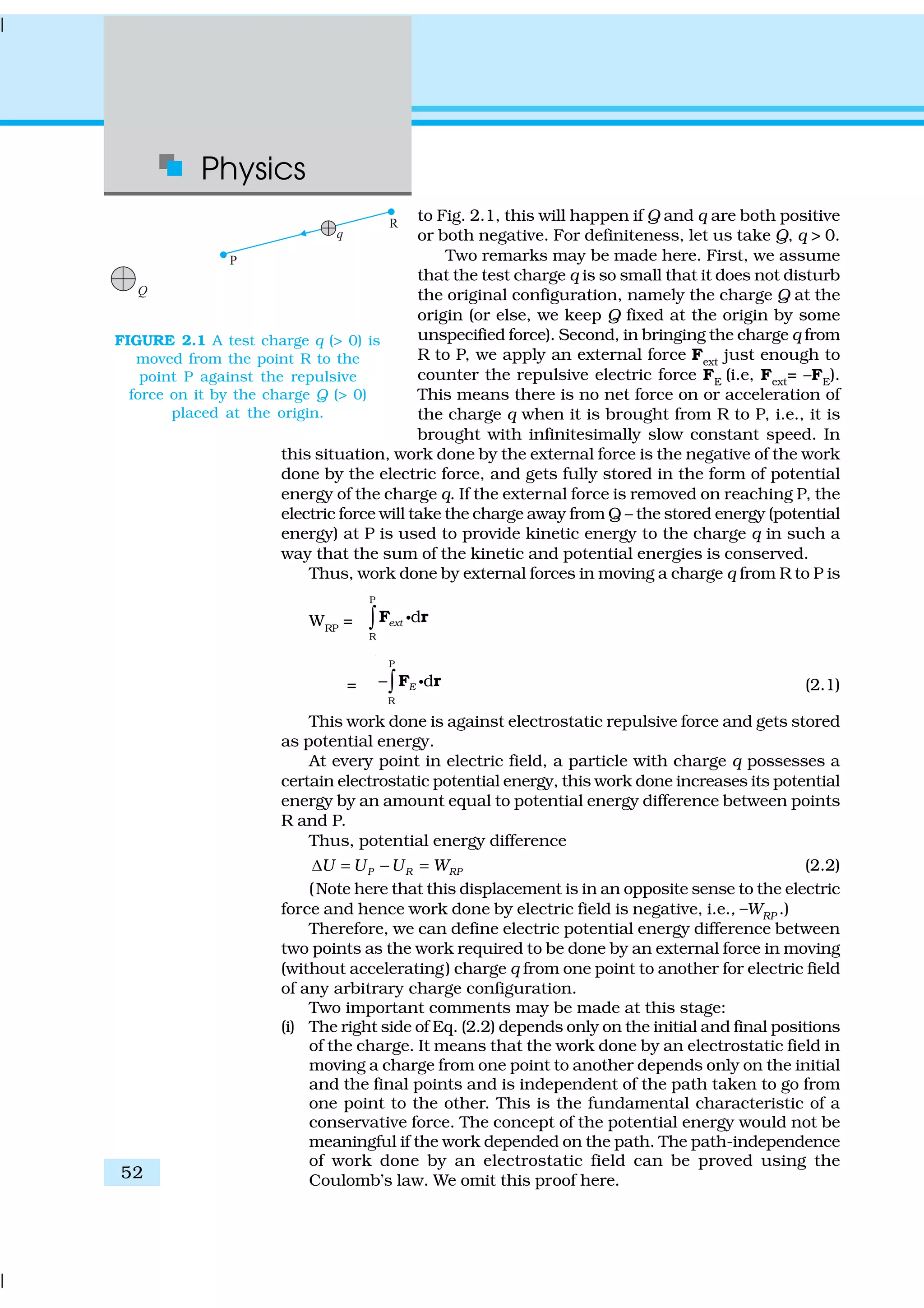
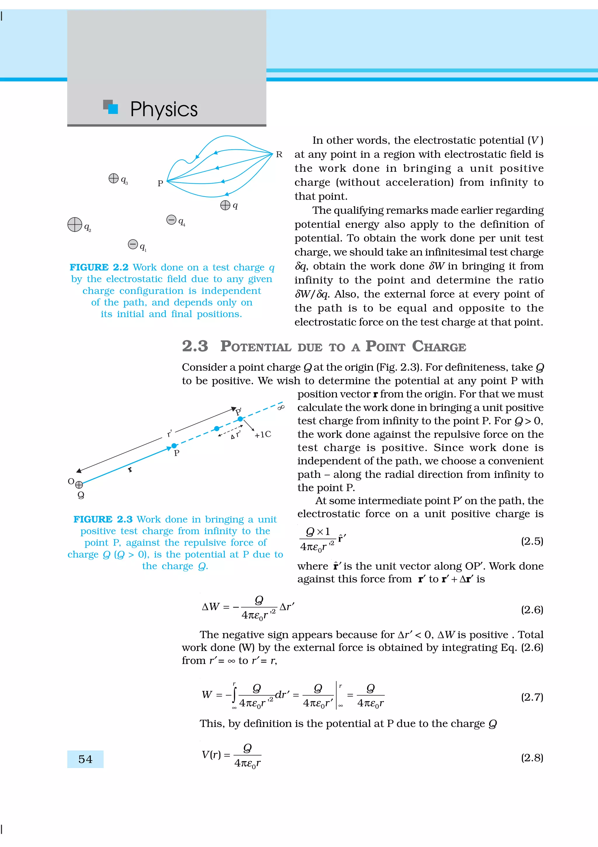
FIGURE 1.1 Rods and pith balls: like charges repel and
unlike charges attract each other.
Interactiveanimationonsimpleelectrostaticexperiments:
http://ephysics.physics.ucla.edu/travoltage/HTML/

7. Electric Charges
and Fields
3
neutralise or nullify each other’s effect. Therefore the charges were named
as positive and negative by the American scientist Benjamin Franklin.
We know that when we add a positive number to a negative number of
the same magnitude, the sum is zero. This might have been the
philosophy in naming the charges as positive and negative. By convention,
the charge on glass rod or cat’s fur is called positive and that on plastic
rod or silk is termed negative. If an object possesses an electric charge, it
is said to be electrified or charged. When it has no charge it is said to be
neutral.
UNIFICATION OF ELECTRICITY AND MAGNETISM
In olden days, electricity and magnetism were treated as separate subjects. Electricity
dealt with charges on glass rods, cat’s fur, batteries, lightning, etc., while magnetism
described interactions of magnets, iron filings, compass needles, etc. In 1820 Danish
scientist Oersted found that a compass needle is deflected by passing an electric current
through a wire placed near the needle. Ampere and Faraday supported this observation
by saying that electric charges in motion produce magnetic fields and moving magnets
generate electricity. The unification was achieved when the Scottish physicist Maxwell
and the Dutch physicist Lorentz put forward a theory where they showed the
interdependence of these two subjects. This field is called electromagnetism. Most of the
phenomena occurring around us can be described under electromagnetism. Virtually
every force that we can think of like friction, chemical force between atoms holding the
matter together, and even the forces describing processes occurring in cells of living
organisms, have its origin in electromagnetic force. Electromagnetic force is one of the
fundamental forces of nature.
Maxwell put forth four equations that play the same role in classical electromagnetism
as Newton’s equations of motion and gravitation law play in mechanics. He also argued
that light is electromagnetic in nature and its speed can be found by making purely
electric and magnetic measurements. He claimed that the science of optics is intimately
related to that of electricity and magnetism.
The science of electricity and magnetism is the foundation for the modern technological
civilisation. Electric power, telecommunication, radio and television, and a wide variety
of the practical appliances used in daily life are based on the principles of this science.
Although charged particles in motion exert both electric and magnetic forces, in the
frame of reference where all the charges are at rest, the forces are purely electrical. You
know that gravitational force is a long-range force. Its effect is felt even when the distance
between the interacting particles is very large because the force decreases inversely as
the square of the distance between the interacting bodies. We will learn in this chapter
that electric force is also as pervasive and is in fact stronger than the gravitational force
by several orders of magnitude (refer to Chapter 1 of Class XI Physics Textbook).
A simple apparatus to detect charge on a body is the gold-leaf
electroscope [Fig. 1.2(a)]. It consists of a vertical metal rod housed in a
box, with two thin gold leaves attached to its bottom end. When a charged
object touches the metal knob at the top of the rod, charge flows on to
the leaves and they diverge. The degree of divergance is an indicator of
the amount of charge.

8. 4
Physics
Students can make a simple electroscope as
follows [Fig. 1.2(b)]: Take a thin aluminium curtain
rod with ball ends fitted for hanging the curtain. Cut
out a piece of length about 20 cm with the ball at
one end and flatten the cut end. Take a large bottle
that can hold this rod and a cork which will fit in the
opening of the bottle. Make a hole in the cork
sufficient to hold the curtain rod snugly. Slide the
rod through the hole in the cork with the cut end on
the lower side and ball end projecting above the cork.
Fold a small, thin aluminium foil (about 6 cm in
length) in the middle and attach it to the flattened
end of the rod by cellulose tape. This forms the leaves
of your electroscope. Fit the cork in the bottle with
about 5 cm of the ball end projecting above the cork.
A paper scale may be put inside the bottle in advance
to measure the separation of leaves. The separation
is a rough measure of the amount of charge on the
electroscope.
To understand how the electroscope works, use
the white paper strips we used for seeing the
attraction of charged bodies. Fold the strips into half
so that you make a mark of fold. Open the strip and
iron it lightly with the mountain fold up, as shown
in Fig. 1.3. Hold the strip by pinching it at the fold.
You would notice that the two halves move apart.
This shows that the strip has acquired charge on ironing. When you fold
it into half, both the halves have the same charge. Hence they repel each
other. The same effect is seen in the leaf electroscope. On charging the
curtain rod by touching the ball end with an electrified body, charge is
transferred to the curtain rod and the attached aluminium foil. Both the
halves of the foil get similar charge and therefore repel each other. The
divergence in the leaves depends on the amount of charge on them. Let
us first try to understand why material bodies acquire charge.
You know that all matter is made up of atoms and/or molecules.
Although normally the materials are electrically neutral, they do contain
charges; but their charges are exactly balanced. Forces that hold the
molecules together, forces that hold atoms together in a solid, the adhesive
force of glue, forces associated with surface tension, all are basically
electrical in nature, arising from the forces between charged particles.
Thus the electric force is all pervasive and it encompasses almost each
and every field associated with our life. It is therefore essential that we
learn more about such a force.
To electrify a neutral body, we need to add or remove one kind of
charge. When we say that a body is charged, we always refer to this
excess charge or deficit of charge. In solids, some of the electrons, being
less tightly bound in the atom, are the charges which are transferred
from one body to the other. A body can thus be charged positively by
losing some of its electrons. Similarly, a body can be charged negatively
FIGURE 1.2 Electroscopes: (a) The gold leaf
electroscope, (b) Schematics of a simple
electroscope.
FIGURE 1.3 Paper strip
experiment.

9. Electric Charges
and Fields
5
by gaining electrons. When we rub a glass rod with silk, some of the
electrons from the rod are transferred to the silk cloth. Thus the rod gets
positively charged and the silk gets negatively charged. No new charge is
created in the process of rubbing. Also the number of electrons, that are
transferred, is a very small fraction of the total number of electrons in the
material body. Also only the less tightly bound electrons in a material
body can be transferred from it to another by rubbing. Therefore, when
a body is rubbed with another, the bodies get charged and that is why
we have to stick to certain pairs of materials to notice charging on rubbing
the bodies.
1.3 CONDUCTORS AND INSULATORS
A metal rod held in hand and rubbed with wool will not show any sign of
being charged. However, if a metal rod with a wooden or plastic handle is
rubbed without touching its metal part, it shows signs of charging.
Suppose we connect one end of a copper wire to a neutral pith ball and
the other end to a negatively charged plastic rod. We will find that the
pith ball acquires a negative charge. If a similar experiment is repeated
with a nylon thread or a rubber band, no transfer of charge will take
place from the plastic rod to the pith ball. Why does the transfer of charge
not take place from the rod to the ball?
Some substances readily allow passage of electricity through them,
others do not. Those which allow electricity to pass through them easily
are called conductors. They have electric charges (electrons) that are
comparatively free to move inside the material. Metals, human and animal
bodies and earth are conductors. Most of the non-metals like glass,
porcelain, plastic, nylon, wood offer high resistance to the passage of
electricity through them. They are called insulators. Most substances
fall into one of the two classes stated above*.
When some charge is transferred to a conductor, it readily gets
distributed over the entire surface of the conductor. In contrast, if some
charge is put on an insulator, it stays at the same place. You will learn
why this happens in the next chapter.
This property of the materials tells you why a nylon or plastic comb
gets electrified on combing dry hair or on rubbing, but a metal article
like spoon does not. The charges on metal leak through our body to the
ground as both are conductors of electricity.
When we bring a charged body in contact with the earth, all the
excess charge on the body disappears by causing a momentary current
to pass to the ground through the connecting conductor (such as our
body). This process of sharing the charges with the earth is called
grounding or earthing. Earthing provides a safety measure for electrical
circuits and appliances. A thick metal plate is buried deep into the earth
and thick wires are drawn from this plate; these are used in buildings
for the purpose of earthing near the mains supply. The electric wiring in
our houses has three wires: live, neutral and earth. The first two carry
* There is a third category called semiconductors, which offer resistance to the
movement of charges which is intermediate between the conductors and
insulators.

10. 6
Physics
electric current from the power station and the third is earthed by
connecting it to the buried metal plate. Metallic bodies of the electric
appliances such as electric iron, refrigerator, TV are connected to the
earth wire. When any fault occurs or live wire touches the metallic body,
the charge flows to the earth without damaging the appliance and without
causing any injury to the humans; this would have otherwise been
unavoidable since the human body is a conductor of electricity.
1.4 CHARGING BY INDUCTION
When we touch a pith ball with an electrified plastic rod, some of the
negative charges on the rod are transferred to the pith ball and it also
gets charged. Thus the pith ball is charged by contact. It is then repelled
by the plastic rod but is attracted by a glass rod which is oppositely
charged. However, why a electrified rod attracts light objects, is a question
we have still left unanswered. Let us try to understand what could be
happening by performing the following experiment.
(i) Bring two metal spheres, A and B, supported on insulating stands,
in contact as shown in Fig. 1.4(a).
(ii) Bring a positively charged rod near one of the spheres, say A, taking
care that it does not touch the sphere. The free electrons in the spheres
are attracted towards the rod. This leaves an excess of positive charge
on the rear surface of sphere B. Both kinds of charges are bound in
the metal spheres and cannot escape. They, therefore, reside on the
surfaces, as shown in Fig. 1.4(b). The left surface of sphere A, has an
excess of negative charge and the right surface of sphere B, has an
excess of positive charge. However, not all of the electrons in the spheres
have accumulated on the left surface of A. As the negative charge
starts building up at the left surface of A, other electrons are repelled
by these. In a short time, equilibrium is reached under the action of
force of attraction of the rod and the force of repulsion due to the
accumulated charges. Fig. 1.4(b) shows the equilibrium situation.
The process is called induction of charge and happens almost
instantly. The accumulated charges remain on the surface, as shown,
till the glass rod is held near the sphere. If the rod is removed, the
charges are not acted by any outside force and they redistribute to
their original neutral state.
(iii) Separate the spheres by a small distance while the glass rod is still
held near sphere A, as shown in Fig. 1.4(c). The two spheres are found
to be oppositely charged and attract each other.
(iv) Remove the rod. The charges on spheres rearrange themselves as
shown in Fig. 1.4(d). Now, separate the spheres quite apart. The
charges on them get uniformly distributed over them, as shown in
Fig. 1.4(e).
In this process, the metal spheres will each be equal and oppositely
charged. This is charging by induction. The positively charged glass rod
does not lose any of its charge, contrary to the process of charging by
contact.
When electrified rods are brought near light objects, a similar effect
takes place. The rods induce opposite charges on the near surfaces of
the objects and similar charges move to the farther side of the object.
FIGURE 1.4 Charging
by induction.

11. Electric Charges
and Fields
7
EXAMPLE1.1
[This happens even when the light object is not a conductor. The
mechanism for how this happens is explained later in Sections 1.10 and
2.10.] The centres of the two types of charges are slightly separated. We
know that opposite charges attract while similar charges repel. However,
the magnitude of force depends on the distance between the charges
and in this case the force of attraction overweighs the force of repulsion.
As a result the particles like bits of paper or pith balls, being light, are
pulled towards the rods.
Example 1.1 How can you charge a metal sphere positively without
touching it?
Solution Figure 1.5(a) shows an uncharged metallic sphere on an
insulating metal stand. Bring a negatively charged rod close to the
metallic sphere, as shown in Fig. 1.5(b). As the rod is brought close
to the sphere, the free electrons in the sphere move away due to
repulsion and start piling up at the farther end. The near end becomes
positively charged due to deficit of electrons. This process of charge
distribution stops when the net force on the free electrons inside the
metal is zero. Connect the sphere to the ground by a conducting
wire. The electrons will flow to the ground while the positive charges
at the near end will remain held there due to the attractive force of
the negative charges on the rod, as shown in Fig. 1.5(c). Disconnect
the sphere from the ground. The positive charge continues to be
held at the near end [Fig. 1.5(d)]. Remove the electrified rod. The
positive charge will spread uniformly over the sphere as shown in
Fig. 1.5(e).
FIGURE 1.5
In this experiment, the metal sphere gets charged by the process
of induction and the rod does not lose any of its charge.
Similar steps are involved in charging a metal sphere negatively
by induction, by bringing a positively charged rod near it. In this
case the electrons will flow from the ground to the sphere when the
sphere is connected to the ground with a wire. Can you explain why?
Interactiveanimationonchargingatwo-spheresystembyinduction:
http://www.physicsclassroom.com/mmedia/estatics/estaticTOC.html

12. 8
Physics
1.5 BASIC PROPERTIES OF ELECTRIC CHARGE
We have seen that there are two types of charges, namely positive and
negative and their effects tend to cancel each other. Here, we shall now
describe some other properties of the electric charge.
If the sizes of charged bodies are very small as compared to the
distances between them, we treat them as point charges. All the
charge content of the body is assumed to be concentrated at one point
in space.
1.5.1 Additivity of charges
We have not as yet given a quantitative definition of a charge; we shall
follow it up in the next section. We shall tentatively assume that this can
be done and proceed. If a system contains two point charges q1
and q2
,
the total charge of the system is obtained simply by adding algebraically
q1
and q2
, i.e., charges add up like real numbers or they are scalars like
the mass of a body. If a system contains n charges q1, q2, q3, …, qn, then
the total charge of the system is q1
+ q2
+ q3
+ … + qn
. Charge has
magnitude but no direction, similar to the mass. However, there is one
difference between mass and charge. Mass of a body is always positive
whereas a charge can be either positive or negative. Proper signs have to
be used while adding the charges in a system. For example, the
total charge of a system containing five charges +1, +2, –3, +4 and –5,
in some arbitrary unit, is (+1) + (+2) + (–3) + (+4) + (–5) = –1 in the
same unit.
1.5.2 Charge is conserved
We have already hinted to the fact that when bodies are charged by
rubbing, there is transfer of electrons from one body to the other; no new
charges are either created or destroyed. A picture of particles of electric
charge enables us to understand the idea of conservation of charge. When
we rub two bodies, what one body gains in charge the other body loses.
Within an isolated system consisting of many charged bodies, due to
interactions among the bodies, charges may get redistributed but it is
found that the total charge of the isolated system is always conserved.
Conservation of charge has been established experimentally.
It is not possible to create or destroy net charge carried by any isolated
system although the charge carrying particles may be created or destroyed
in a process. Sometimes nature creates charged particles: a neutron turns
into a proton and an electron. The proton and electron thus created have
equal and opposite charges and the total charge is zero before and after
the creation.
1.5.3 Quantisation of charge
Experimentally it is established that all free charges are integral multiples
of a basic unit of charge denoted by e. Thus charge q on a body is always
given by
q = ne

13. Electric Charges
and Fields
9
where n is any integer, positive or negative. This basic unit of charge is
the charge that an electron or proton carries. By convention, the charge
on an electron is taken to be negative; therefore charge on an electron is
written as –e and that on a proton as +e.
The fact that electric charge is always an integral multiple of e is termed
as quantisation of charge. There are a large number of situations in physics
where certain physical quantities are quantised. The quantisation of charge
was first suggested by the experimental laws of electrolysis discovered by
English experimentalist Faraday. It was experimentally demonstrated by
Millikan in 1912.
In the International System (SI) of Units, a unit of charge is called a
coulomb and is denoted by the symbol C. A coulomb is defined in terms
the unit of the electric current which you are going to learn in a
subsequent chapter. In terms of this definition, one coulomb is the charge
flowing through a wire in 1 s if the current is 1 A (ampere), (see Chapter 2
of Class XI, Physics Textbook , Part I). In this system, the value of the
basic unit of charge is
e = 1.602192 × 10–19
C
Thus, there are about 6 × 1018
electrons in a charge of –1C. In
electrostatics, charges of this large magnitude are seldom encountered
and hence we use smaller units 1 μC (micro coulomb) = 10–6
C or 1 mC
(milli coulomb) = 10–3
C.
If the protons and electrons are the only basic charges in the universe,
all the observable charges have to be integral multiples of e. Thus, if a
body contains n1
electrons and n2
protons, the total amount of charge
on the body is n2
× e + n1
× (–e) = (n2
– n1
) e. Since n1
and n2
are integers,
their difference is also an integer. Thus the charge on any body is always
an integral multiple of e and can be increased or decreased also in steps
of e.
The step size e is, however, very small because at the macroscopic
level, we deal with charges of a few μC. At this scale the fact that charge of
a body can increase or decrease in units of e is not visible. The grainy
nature of the charge is lost and it appears to be continuous.
This situation can be compared with the geometrical concepts of points
and lines. A dotted line viewed from a distance appears continuous to
us but is not continuous in reality. As many points very close to
each other normally give an impression of a continuous line, many
small charges taken together appear as a continuous charge
distribution.
At the macroscopic level, one deals with charges that are enormous
compared to the magnitude of charge e. Since e = 1.6 × 10–19
C, a charge
of magnitude, say 1 μC, contains something like 1013
times the electronic
charge. At this scale, the fact that charge can increase or decrease only in
units of e is not very different from saying that charge can take continuous
values. Thus, at the macroscopic level, the quantisation of charge has no
practical consequence and can be ignored. At the microscopic level, where
the charges involved are of the order of a few tens or hundreds of e, i.e.,

14. 10
Physics
EXAMPLE1.3EXAMPLE1.2
they can be counted, they appear in discrete lumps and quantisation of
charge cannot be ignored. It is the scale involved that is very important.
Example 1.2 If 109
electrons move out of a body to another body
every second, how much time is required to get a total charge of 1 C
on the other body?
Solution In one second 109
electrons move out of the body. Therefore
the charge given out in one second is 1.6 × 10–19
× 109
C = 1.6 × 10–10
C.
The time required to accumulate a charge of 1 C can then be estimated
to be 1 C ÷ (1.6 × 10–10
C/s) = 6.25 × 109
s = 6.25 × 109
÷ (365 × 24 ×
3600) years = 198 years. Thus to collect a charge of one coulomb,
from a body from which 109
electrons move out every second, we will
need approximately 200 years. One coulomb is, therefore, a very large
unit for many practical purposes.
It is, however, also important to know what is roughly the number of
electrons contained in a piece of one cubic centimetre of a material.
A cubic piece of copper of side 1 cm contains about 2.5 × 1024
electrons.
Example 1.3 How much positive and negative charge is there in a
cup of water?
Solution Let us assume that the mass of one cup of water is
250 g. The molecular mass of water is 18g. Thus, one mole
(= 6.02 × 1023
molecules) of water is 18 g. Therefore the number of
molecules in one cup of water is (250/18) × 6.02 × 1023
.
Each molecule of water contains two hydrogen atoms and one oxygen
atom, i.e., 10 electrons and 10 protons. Hence the total positive and
total negative charge has the same magnitude. It is equal to
(250/18) × 6.02 × 1023
× 10 × 1.6 × 10–19
C = 1.34 × 107
C.
1.6 COULOMB’S LAW
Coulomb’s law is a quantitative statement about the force between two
point charges. When the linear size of charged bodies are much smaller
than the distance separating them, the size may be ignored and the
charged bodies are treated as point charges. Coulomb measured the
force between two point charges and found that it varied inversely as
the square of the distance between the charges and was directly
proportional to the product of the magnitude of the two charges and
acted along the line joining the two charges. Thus, if two point charges
q1, q2 are separated by a distance r in vacuum, the magnitude of the
force (F) between them is given by
21
2
q q
F k
r
= (1.1)
How did Coulomb arrive at this law from his experiments? Coulomb
used a torsion balance* for measuring the force between two charged metallic
* A torsion balance is a sensitive device to measure force. It was also used later
by Cavendish to measure the very feeble gravitational force between two objects,
to verify Newton’s Law of Gravitation.

15. Electric Charges
and Fields
11
spheres. When the separation between two spheres is much
larger than the radius of each sphere, the charged spheres
may be regarded as point charges. However, the charges
on the spheres were unknown, to begin with. How then
could he discover a relation like Eq. (1.1)? Coulomb
thought of the following simple way: Suppose the charge
on a metallic sphere is q. If the sphere is put in contact
with an identical uncharged sphere, the charge will spread
over the two spheres. By symmetry, the charge on each
sphere will be q/2*. Repeating this process, we can get
charges q/2, q/4, etc. Coulomb varied the distance for a
fixed pair of charges and measured the force for different
separations. He then varied the charges in pairs, keeping
the distance fixed for each pair. Comparing forces for
different pairs of charges at different distances, Coulomb
arrived at the relation, Eq. (1.1).
Coulomb’s law, a simple mathematical statement,
was initially experimentally arrived at in the manner
described above. While the original experiments
established it at a macroscopic scale, it has also been
established down to subatomic level (r ~ 10–10
m).
Coulomb discovered his law without knowing the
explicit magnitude of the charge. In fact, it is the other
way round: Coulomb’s law can now be employed to
furnish a definition for a unit of charge. In the relation,
Eq. (1.1), k is so far arbitrary. We can choose any positive
value of k. The choice of k determines the size of the unit
of charge. In SI units, the value of k is about 9 × 109
.
The unit of charge that results from this choice is called
a coulomb which we defined earlier in Section 1.4.
Putting this value of k in Eq. (1.1), we see that for
q1
= q2
= 1 C, r = 1 m
F = 9 × 109
N
That is, 1 C is the charge that when placed at a
distance of 1 m from another charge of the same
magnitude in vacuum experiences an electrical force of
repulsion of magnitude 9 × 109
N. One coulomb is
evidently too big a unit to be used. In practice, in
electrostatics, one uses smaller units like 1 mC or 1 μC.
The constant k in Eq. (1.1) is usually put as
k = 1/4πε0
for later convenience, so that Coulomb’s law is written as
0
1 2
2
1
4
q q
F
rε
=
π
(1.2)
ε0
is called the permittivity of free space . The value of ε0
in SI units is
0ε = 8.854 × 10–12
C2
N–1
m–2
* Implicit in this is the assumption of additivity of charges and conservation:
two charges (q/2 each) add up to make a total charge q.
Charles Augustin de
Coulomb (1736 – 1806)
Coulomb, a French
physicist, began his career
as a military engineer in
the West Indies. In 1776, he
returned to Paris and
retired to a small estate to
do his scientific research.
He invented a torsion
balance to measure the
quantity of a force and used
it for determination of
forces of electric attraction
or repulsion between small
charged spheres. He thus
arrived in 1785 at the
inverse square law relation,
now known as Coulomb’s
law. The law had been
anticipated by Priestley and
also by Cavendish earlier,
though Cavendish never
published his results.
Coulomb also found the
inverse square law of force
between unlike and like
magnetic poles.
CHARLESAUGUSTINDECOULOMB(1736–1806)

16. 12
Physics
Since force is a vector, it is better to write
Coulomb’s law in the vector notation. Let the
position vectors of charges q1
and q2
be r1
and r2
respectively [see Fig.1.6(a)]. We denote force on
q1
due to q2
by F12
and force on q2
due to q1
by
F21
. The two point charges q1
and q2
have been
numbered 1 and 2 for convenience and the vector
leading from 1 to 2 is denoted by r21
:
r21
= r2
– r1
In the same way, the vector leading from 2 to
1 is denoted by r12
:
r12
= r1
– r2
= – r21
The magnitude of the vectors r21
and r12
is
denoted by r21
and r12
, respectively (r12
= r21
). The
direction of a vector is specified by a unit vector
along the vector. To denote the direction from 1
to 2 (or from 2 to 1), we define the unit vectors:
21
21
21
ˆ
r
=
r
r ,
12
12 21 12
12
ˆ ˆ ˆ,
r
= =
r
r r r
Coulomb’s force law between two point charges q1 and q2 located at
r1 and r2 is then expressed as
1 2
21 212
21
1
ˆ
4 o
q q
rε
=
π
F r (1.3)
Some remarks on Eq. (1.3) are relevant:
• Equation (1.3) is valid for any sign of q1
and q2
whether positive or
negative. If q1 and q2 are of the same sign (either both positive or both
negative), F21
is along ˆr 21
, which denotes repulsion, as it should be for
like charges. If q1
and q2
are of opposite signs, F21
is along – ˆr 21
(= ˆr 12
),
which denotes attraction, as expected for unlike charges. Thus, we do
not have to write separate equations for the cases of like and unlike
charges. Equation (1.3) takes care of both cases correctly [Fig. 1.6(b)].
• The force F12 on charge q1 due to charge q2, is obtained from Eq. (1.3),
by simply interchanging 1 and 2, i.e.,
1 2
12 12 212
0 12
1
ˆ
4
q q
rε
= = −
π
F r F
Thus, Coulomb’s law agrees with the Newton’s third law.
• Coulomb’s law [Eq. (1.3)] gives the force between two charges q1
and
q2 in vacuum. If the charges are placed in matter or the intervening
space has matter, the situation gets complicated due to the presence
of charged constituents of matter. We shall consider electrostatics in
matter in the next chapter.
FIGURE 1.6 (a) Geometry and
(b) Forces between charges.

17. Electric Charges
and Fields
13
EXAMPLE1.4
Example 1.4 Coulomb’s law for electrostatic force between two point
charges and Newton’s law for gravitational force between two
stationary point masses, both have inverse-square dependence on
the distance between the charges/masses. (a) Compare the strength
of these forces by determining the ratio of their magnitudes (i) for an
electron and a proton and (ii) for two protons. (b) Estimate the
accelerations of electron and proton due to the electrical force of their
mutual attraction when they are 1 Å (= 10-10
m) apart? (mp
= 1.67 ×
10–27
kg, me
= 9.11 × 10–31
kg)
Solution
(a) (i) The electric force between an electron and a proton at a distance
r apart is:
2
2
0
1
4
e
e
F
rε
= −
π
where the negative sign indicates that the force is attractive. The
corresponding gravitational force (always attractive) is:
2
p e
G
m m
F G
r
= −
where mp
and me
are the masses of a proton and an electron
respectively.
2
39
0
2.4 10
4
e
G p e
F e
F Gm mε
= = ×
π
(ii) On similar lines, the ratio of the magnitudes of electric force
to the gravitational force between two protons at a distance r
apart is :
2
04
e
G p p
F e
F Gm mε
= =
π
1.3 × 1036
However, it may be mentioned here that the signs of the two forces
are different. For two protons, the gravitational force is attractive
in nature and the Coulomb force is repulsive . The actual values
of these forces between two protons inside a nucleus (distance
between two protons is ~ 10-15
m inside a nucleus) are Fe
~ 230 N
whereas FG
~ 1.9 × 10–34
N.
The (dimensionless) ratio of the two forces shows that electrical
forces are enormously stronger than the gravitational forces.
(b) The electric force F exerted by a proton on an electron is same in
magnitude to the force exerted by an electron on a proton; however
the masses of an electron and a proton are different. Thus, the
magnitude of force is
|F| =
2
2
0
1
4
e
rεπ
= 8.987 × 109
Nm2
/C2
× (1.6 ×10–19
C)2
/ (10–10
m)2
= 2.3 × 10–8
N
Using Newton’s second law of motion, F = ma, the acceleration
that an electron will undergo is
a = 2.3×10–8
N / 9.11 ×10–31
kg = 2.5 × 1022
m/s2
Comparing this with the value of acceleration due to gravity, we
can conclude that the effect of gravitational field is negligible on
the motion of electron and it undergoes very large accelerations
under the action of Coulomb force due to a proton.
The value for acceleration of the proton is
2.3 × 10–8
N / 1.67 × 10–27
kg = 1.4 × 1019
m/s2
InteractiveanimationonCoulomb’slaw:
http://webphysics.davidson.edu/physlet_resources/bu_semester2/co1_coulomb.html

18. 14
Physics
EXAMPLE1.5
Example 1.5 A charged metallic sphere A is suspended by a nylon
thread. Another charged metallic sphere B held by an insulating
handle is brought close to A such that the distance between their
centres is 10 cm, as shown in Fig. 1.7(a). The resulting repulsion of A
is noted (for example, by shining a beam of light and measuring the
deflection of its shadow on a screen). Spheres A and B are touched
by uncharged spheres C and D respectively, as shown in Fig. 1.7(b).
C and D are then removed and B is brought closer to A to a
distance of 5.0 cm between their centres, as shown in Fig. 1.7(c).
What is the expected repulsion of A on the basis of Coulomb’s law?
Spheres A and C and spheres B and D have identical sizes. Ignore
the sizes of A and B in comparison to the separation between their
centres.
FIGURE 1.7

19. Electric Charges
and Fields
15
EXAMPLE1.5
Solution Let the original charge on sphere A be q and that on B be
q′. At a distance r between their centres, the magnitude of the
electrostatic force on each is given by
2
0
1
4
qq
F
rε
′
=
π
neglecting the sizes of spheres A and B in comparison to r. When an
identical but uncharged sphere C touches A, the charges redistribute
on A and C and, by symmetry, each sphere carries a charge q/2.
Similarly, after D touches B, the redistributed charge on each is
q′/2. Now, if the separation between A and B is halved, the magnitude
of the electrostatic force on each is
2 2
0 0
1 ( /2)( /2) 1 ( )
4 4( /2)
q q qq
F F
r rε ε
′ ′
= = =′
π π
Thus the electrostatic force on A, due to B, remains unaltered.
1.7 FORCES BETWEEN MULTIPLE CHARGES
The mutual electric force between two charges is given
by Coulomb’s law. How to calculate the force on a
charge where there are not one but several charges
around? Consider a system of n stationary charges
q1, q2, q3, ..., qn in vacuum. What is the force on q1 due
to q2
, q3
, ..., qn
? Coulomb’s law is not enough to answer
this question. Recall that forces of mechanical origin
add according to the parallelogram law of addition. Is
the same true for forces of electrostatic origin?
Experimentally it is verified that force on any
charge due to a number of other charges is the vector
sum of all the forces on that charge due to the other
charges, taken one at a time. The individual forces
are unaffected due to the presence of other charges.
This is termed as the principle of superposition.
To better understand the concept, consider a
system of three charges q1, q2 and q3, as shown in
Fig. 1.8(a). The force on one charge, say q1
, due to two
other charges q2
, q3
can therefore be obtained by
performing a vector addition of the forces due to each
one of these charges. Thus, if the force on q1
due to q2
is denoted by F12
, F12
is given by Eq. (1.3) even though
other charges are present.
Thus, F12
1 2
122
0 12
1
ˆ
4
q q
rε
=
π
r
In the same way, the force on q1 due to q3, denoted
by F13
, is given by
1 3
13 132
0 13
1
ˆ
4
q q
rε
=
π
F r
FIGURE 1.8 A system of (a) three
charges (b) multiple charges.

20. 16
Physics
EXAMPLE1.6
which again is the Coulomb force on q1
due to q3
, even though other
charge q2
is present.
Thus the total force F1 on q1 due to the two charges q2 and q3 is
given as
1 31 2
1 12 13 12 132 2
0 012 13
1 1
ˆ ˆ
4 4
q qq q
r rε ε
= + = +
π π
F F F r r (1.4)
The above calculation of force can be generalised to a system of
charges more than three, as shown in Fig. 1.8(b).
The principle of superposition says that in a system of charges q1,
q2
, ..., qn
, the force on q1
due to q2
is the same as given by Coulomb’s law,
i.e., it is unaffected by the presence of the other charges q3
, q4
, ..., qn
. The
total force F1 on the charge q1, due to all other charges, is then given by
the vector sum of the forces F12
, F13
, ..., F1n
:
i.e.,
1 3 11 2
1 12 13 1n 12 13 12 2 2
0 12 13 1
1
ˆ ˆ ˆ= + + ...+ ...
4
n
n
n
q q q qq q
r r rε
⎡ ⎤
= + + +⎢ ⎥
π ⎣ ⎦
F F F F r r r
1
12
20 1
ˆ
4
n
i
i
i i
qq
rε =
=
π
∑ r (1.5)
The vector sum is obtained as usual by the parallelogram law of
addition of vectors. All of electrostatics is basically a consequence of
Coulomb’s law and the superposition principle.
Example 1.6 Consider three charges q1
, q2
, q3
each equal to q at the
vertices of an equilateral triangle of side l. What is the force on a
charge Q (with the same sign as q) placed at the centroid of the
triangle, as shown in Fig. 1.9?
FIGURE 1.9
Solution In the given equilateral triangle ABC of sides of length l, if
we draw a perpendicular AD to the side BC,
AD = AC cos 30º = ( 3 /2 ) l and the distance AO of the centroid O
from A is (2/3) AD = (1/ 3 ) l. By symmatry AO = BO = CO.

21. Electric Charges
and Fields
17
EXAMPLE1.6
Thus,
Force F1
on Q due to charge q at A = 2
0
3
4
Qq
lεπ
along AO
Force F2
on Q due to charge q at B = 2
0
3
4
Qq
lεπ along BO
Force F3
on Q due to charge q at C = 2
0
3
4
Qq
lεπ along CO
The resultant of forces F2
and F3
is 2
0
3
4
Qq
lεπ along OA, by the
parallelogram law. Therefore, the total force on Q = ( )2
0
3
ˆ ˆ
4
Qq
lε
−
π
r r
= 0, where ˆr is the unit vector along OA.
It is clear also by symmetry that the three forces will sum to zero.
Suppose that the resultant force was non-zero but in some direction.
Consider what would happen if the system was rotated through 60º
about O.
Example 1.7 Consider the charges q, q, and –q placed at the vertices
of an equilateral triangle, as shown in Fig. 1.10. What is the force on
each charge?
FIGURE 1.10
Solution The forces acting on charge q at A due to charges q at B
and –q at C are F12
along BA and F13
along AC respectively, as shown
in Fig. 1.10. By the parallelogram law, the total force F1
on the charge
q at A is given by
F1
= F 1ˆr where 1ˆr is a unit vector along BC.
The force of attraction or repulsion for each pair of charges has the
same magnitude
2
2
04
q
F
lε
=
π
The total force F2
on charge q at B is thus F2
= F ˆr 2
, where ˆr 2
is a
unit vector along AC.
EXAMPLE1.7

22. 18
Physics
EXAMPLE1.7
Similarly the total force on charge –q at C is F3
= 3 F ˆn , where ˆn is
the unit vector along the direction bisecting the ∠BCA.
It is interesting to see that the sum of the forces on the three charges
is zero, i.e.,
F1
+ F2
+ F3
= 0
The result is not at all surprising. It follows straight from the fact
that Coulomb’s law is consistent with Newton’s third law. The proof
is left to you as an exercise.
1.8 ELECTRIC FIELD
Let us consider a point charge Q placed in vacuum, at the origin O. If we
place another point charge q at a point P, where OP = r, then the charge Q
will exert a force on q as per Coulomb’s law. We may ask the question: If
charge q is removed, then what is left in the surrounding? Is there
nothing? If there is nothing at the point P, then how does a force act
when we place the charge q at P. In order to answer such questions, the
early scientists introduced the concept of field. According to this, we say
that the charge Q produces an electric field everywhere in the surrounding.
When another charge q is brought at some point P, the field there acts on
it and produces a force. The electric field produced by the charge Q at a
point r is given as
( ) 2 2
0 0
1 1
ˆ ˆ
4 4
Q Q
r rε ε
= =
π π
E r r r (1.6)
where ˆ =r r/r, is a unit vector from the origin to the point r. Thus, Eq.(1.6)
specifies the value of the electric field for each value of the position
vector r. The word “field” signifies how some distributed quantity (which
could be a scalar or a vector) varies with position. The effect of the charge
has been incorporated in the existence of the electric field. We obtain the
force F exerted by a charge Q on a charge q, as
2
0
1
ˆ
4
Qq
rε
=
π
F r (1.7)
Note that the charge q also exerts an equal and opposite force on the
charge Q. The electrostatic force between the charges Q and q can be
looked upon as an interaction between charge q and the electric field of
Q and vice versa. If we denote the position of charge q by the vector r, it
experiences a force F equal to the charge q multiplied by the electric
field E at the location of q. Thus,
F(r) = q E(r) (1.8)
Equation (1.8) defines the SI unit of electric field as N/C*.
Some important remarks may be made here:
(i) From Eq. (1.8), we can infer that if q is unity, the electric field due to
a charge Q is numerically equal to the force exerted by it. Thus, the
electric field due to a charge Q at a point in space may be defined
as the force that a unit positive charge would experience if placed
* An alternate unit V/m will be introduced in the next chapter.
FIGURE 1.11 Electric
field (a) due to a
charge Q, (b) due to a
charge –Q.

23. Electric Charges
and Fields
19
at that point. The charge Q, which is producing the electric field, is
called a source charge and the charge q, which tests the effect of a
source charge, is called a test charge. Note that the source charge Q
must remain at its original location. However, if a charge q is brought
at any point around Q, Q itself is bound to experience an electrical
force due to q and will tend to move. A way out of this difficulty is to
make q negligibly small. The force F is then negligibly small but the
ratio F/q is finite and defines the electric field:
0
lim
q q→
⎛ ⎞
= ⎜ ⎟⎝ ⎠
F
E (1.9)
A practical way to get around the problem (of keeping Q undisturbed
in the presence of q) is to hold Q to its location by unspecified forces!
This may look strange but actually this is what happens in practice.
When we are considering the electric force on a test charge q due to a
charged planar sheet (Section 1.15), the charges on the sheet are held to
their locations by the forces due to the unspecified charged constituents
inside the sheet.
(ii) Note that the electric field E due to Q, though defined operationally
in terms of some test charge q, is independent of q. This is because
F is proportional to q, so the ratio F/q does not depend on q. The
force F on the charge q due to the charge Q depends on the particular
location of charge q which may take any value in the space around
the charge Q. Thus, the electric field E due to Q is also dependent on
the space coordinate r. For different positions of the charge q all over
the space, we get different values of electric field E. The field exists at
every point in three-dimensional space.
(iii) For a positive charge, the electric field will be directed radially
outwards from the charge. On the other hand, if the source charge is
negative, the electric field vector, at each point, points radially inwards.
(iv) Since the magnitude of the force F on charge q due to charge Q
depends only on the distance r of the charge q from charge Q,
the magnitude of the electric field E will also depend only on the
distance r. Thus at equal distances from the charge Q, the magnitude
of its electric field E is same. The magnitude of electric field E due to
a point charge is thus same on a sphere with the point charge at its
centre; in other words, it has a spherical symmetry.
1.8.1 Electric field due to a system of charges
Consider a system of charges q1
, q2
, ..., qn
with position vectors r1
,
r2
, ..., rn
relative to some origin O. Like the electric field at a point in
space due to a single charge, electric field at a point in space due to the
system of charges is defined to be the force experienced by a unit
test charge placed at that point, without disturbing the original
positions of charges q1
, q2
, ..., qn
. We can use Coulomb’s law and the
superposition principle to determine this field at a point P denoted by
position vector r.

24. 20
Physics
Electric field E1
at r due to q1
at r1
is given by
E1
= 1
1P2
0 1P
1
ˆ
4
q
rπε
r
where 1P
ˆr is a unit vector in the direction from q1 to P,
and r1P
is the distance between q1
and P.
In the same manner, electric field E2 at r due to q2 at
r2 is
E2
=
2
2P2
0 2P
1
ˆ
4
q
rπε
r
where 2P
ˆr is a unit vector in the direction from q2 to P
and r2P
is the distance between q2
and P. Similar
expressions hold good for fields E3
, E4
, ..., En
due to
charges q3, q4, ..., qn.
By the superposition principle, the electric field E at r
due to the system of charges is (as shown in Fig. 1.12)
E(r) = E1 (r) + E2 (r) + … + En(r)
= 1 2
1P 2P P2 2 2
0 0 01P 2P P
1 1 1
ˆ ˆ ˆ...
4 4 4
n
n
n
qq q
r r rε ε ε
+ + +
π π π
r r r
E(r) i P2
10 P
1
ˆ
4
n
i
i i
q
rε =
=
π
∑ r (1.10)
E is a vector quantity that varies from one point to another point in space
and is determined from the positions of the source charges.
1.8.2 Physical significance of electric field
You may wonder why the notion of electric field has been introduced
here at all. After all, for any system of charges, the measurable quantity
is the force on a charge which can be directly determined using Coulomb’s
law and the superposition principle [Eq. (1.5)]. Why then introduce this
intermediate quantity called the electric field?
For electrostatics, the concept of electric field is convenient, but not
really necessary. Electric field is an elegant way of characterising the
electrical environment of a system of charges. Electric field at a point in
the space around a system of charges tells you the force a unit positive
test charge would experience if placed at that point (without disturbing
the system). Electric field is a characteristic of the system of charges and
is independent of the test charge that you place at a point to determine
the field. The term field in physics generally refers to a quantity that is
defined at every point in space and may vary from point to point. Electric
field is a vector field, since force is a vector quantity.
The true physical significance of the concept of electric field, however,
emerges only when we go beyond electrostatics and deal with time-
dependent electromagnetic phenomena. Suppose we consider the force
between two distant charges q1, q2 in accelerated motion. Now the greatest
speed with which a signal or information can go from one point to another
is c, the speed of light. Thus, the effect of any motion of q1
on q2
cannot
FIGURE 1.12 Electric field at a
point due to a system of charges is
the vector sum of the electric fields
at the point due to individual
charges.

25. Electric Charges
and Fields
21
arise instantaneously. There will be some time delay between the effect
(force on q2
) and the cause (motion of q1
). It is precisely here that the
notion of electric field (strictly, electromagnetic field) is natural and very
useful. The field picture is this: the accelerated motion of charge q1
produces electromagnetic waves, which then propagate with the speed
c, reach q2 and cause a force on q2. The notion of field elegantly accounts
for the time delay. Thus, even though electric and magnetic fields can be
detected only by their effects (forces) on charges, they are regarded as
physical entities, not merely mathematical constructs. They have an
independent dynamics of their own, i.e., they evolve according to laws
of their own. They can also transport energy. Thus, a source of time-
dependent electromagnetic fields, turned on briefly and switched off, leaves
behind propagating electromagnetic fields transporting energy. The
concept of field was first introduced by Faraday and is now among the
central concepts in physics.
Example 1.8 An electron falls through a distance of 1.5 cm in a
uniform electric field of magnitude 2.0 × 104
N C–1
[Fig. 1.13(a)]. The
direction of the field is reversed keeping its magnitude unchanged
and a proton falls through the same distance [Fig. 1.13(b)]. Compute
the time of fall in each case. Contrast the situation with that of ‘free
fall under gravity’.
FIGURE 1.13
Solution In Fig. 1.13(a) the field is upward, so the negatively charged
electron experiences a downward force of magnitude eE where E is
the magnitude of the electric field. The acceleration of the electron is
ae
= eE/me
where me
is the mass of the electron.
Starting from rest, the time required by the electron to fall through a
distance h is given by
22
e
e
e
h mh
t
a e E
= =
For e = 1.6 × 10–19
C, me
= 9.11 × 10–31
kg,
E = 2.0 × 104
N C–1
, h = 1.5 × 10–2
m,
te
= 2.9 × 10–9
s
In Fig. 1.13 (b), the field is downward, and the positively charged
proton experiences a downward force of magnitude eE. The
acceleration of the proton is
ap
= eE/mp
where mp
is the mass of the proton; mp
= 1.67 × 10–27
kg. The time of
fall for the proton is
EXAMPLE1.8

26. 22
Physics
EXAMPLE1.9EXAMPLE1.8
–7
22
1 3 10 s
p
p
p
h mh
t .
a e E
= = = ×
Thus, the heavier particle (proton) takes a greater time to fall through
the same distance. This is in basic contrast to the situation of ‘free
fall under gravity’ where the time of fall is independent of the mass of
the body. Note that in this example we have ignored the acceleration
due to gravity in calculating the time of fall. To see if this is justified,
let us calculate the acceleration of the proton in the given electric
field:
p
p
e E
a
m
=
19 4 1
27
(1 6 10 C) (2 0 10 N C )
1 67 10 kg
. .
.
− −
−
× × ×
=
×
12 –2
1 9 10 m s.= ×
which is enormous compared to the value of g (9.8 m s–2
), the
acceleration due to gravity. The acceleration of the electron is even
greater. Thus, the effect of acceleration due to gravity can be ignored
in this example.
Example 1.9 Two point charges q1
and q2
, of magnitude +10–8
C and
–10–8
C, respectively, are placed 0.1 m apart. Calculate the electric
fields at points A, B and C shown in Fig. 1.14.
FIGURE 1.14
Solution The electric field vector E1A
at A due to the positive charge
q1
points towards the right and has a magnitude
9 2 -2 8
1A 2
(9 10 Nm C ) (10 C)
(0.05m)
E
−
× ×
= = 3.6 × 104
N C–1
The electric field vector E2A
at A due to the negative charge q2
points
towards the right and has the same magnitude. Hence the magnitude
of the total electric field EA
at A is
EA
= E1A
+ E2A
= 7.2 × 104
N C–1
EA
is directed toward the right.

27. Electric Charges
and Fields
23
The electric field vector E1B
at B due to the positive charge q1
points
towards the left and has a magnitude
9 2 –2 8
1B 2
(9 10 Nm C ) (10 C)
(0.05 m)
E
−
× ×
= = 3.6 × 104
N C–1
The electric field vector E2B
at B due to the negative charge q2
points
towards the right and has a magnitude
9 2 –2 8
2B 2
(9 10 Nm C ) (10 C)
(0.15 m)
E
−
× ×
= = 4 × 103
N C–1
The magnitude of the total electric field at B is
EB
= E1B
– E2B
= 3.2 × 104
N C–1
EB
is directed towards the left.
The magnitude of each electric field vector at point C, due to charge
q1
and q2
is
9 2 –2 8
1C 2C 2
(9 10 Nm C ) (10 C)
(0.10 m)
E E
−
× ×
= = = 9 × 103
N C–1
The directions in which these two vectors point are indicated in
Fig. 1.14. The resultant of these two vectors is
1 2cos cos
3 3
CE E E
π π
= + = 9 × 103
N C–1
EC
points towards the right.
1.9 ELECTRIC FIELD LINES
We have studied electric field in the last section. It is a vector quantity
and can be represented as we represent vectors. Let us try to represent E
due to a point charge pictorially. Let the point charge be placed at the
origin. Draw vectors pointing along the direction of the electric field with
their lengths proportional to the strength of the field at
each point. Since the magnitude of electric field at a point
decreases inversely as the square of the distance of that
point from the charge, the vector gets shorter as one goes
away from the origin, always pointing radially outward.
Figure 1.15 shows such a picture. In this figure, each
arrow indicates the electric field, i.e., the force acting on a
unit positive charge, placed at the tail of that arrow.
Connect the arrows pointing in one direction and the
resulting figure represents a field line. We thus get many
field lines, all pointing outwards from the point charge.
Have we lost the information about the strength or
magnitude of the field now, because it was contained in
the length of the arrow? No. Now the magnitude of the
field is represented by the density of field lines. E is strong
near the charge, so the density of field lines is more near
the charge and the lines are closer. Away from the charge,
the field gets weaker and the density of field lines is less,
resulting in well-separated lines.
Another person may draw more lines. But the number of lines is not
important. In fact, an infinite number of lines can be drawn in any region.
FIGURE 1.15 Field of a point charge.
EXAMPLE1.9

28. 24
Physics
It is the relative density of lines in different regions which is
important.
We draw the figure on the plane of paper, i.e., in two-
dimensions but we live in three-dimensions. So if one wishes
to estimate the density of field lines, one has to consider the
number of lines per unit cross-sectional area, perpendicular
to the lines. Since the electric field decreases as the square of
the distance from a point charge and the area enclosing the
charge increases as the square of the distance, the number
of field lines crossing the enclosing area remains constant,
whatever may be the distance of the area from the charge.
We started by saying that the field lines carry information
about the direction of electric field at different points in space.
Having drawn a certain set of field lines, the relative density
(i.e., closeness) of the field lines at different points indicates
the relative strength of electric field at those points. The field
lines crowd where the field is strong and are spaced apart
where it is weak. Figure 1.16 shows a set of field lines. We
can imagine two equal and small elements of area placed at points R and
S normal to the field lines there. The number of field lines in our picture
cutting the area elements is proportional to the magnitude of field at
these points. The picture shows that the field at R is stronger than at S.
To understand the dependence of the field lines on the area, or rather
the solid angle subtended by an area element, let us try to relate the
area with the solid angle, a generalization of angle to three dimensions.
Recall how a (plane) angle is defined in two-dimensions. Let a small
transverse line element Δl be placed at a distance r from a point O. Then
the angle subtended by Δl at O can be approximated as Δθ = Δl/r.
Likewise, in three-dimensions the solid angle* subtended by a small
perpendicular plane area ΔS, at a distance r, can be written as
ΔΩ = ΔS/r2
. We know that in a given solid angle the number of radial
field lines is the same. In Fig. 1.16, for two points P1
and P2
at distances
r1 and r2 from the charge, the element of area subtending the solid angle
ΔΩ is 2
1r ΔΩ at P1
and an element of area 2
2r ΔΩ at P2
, respectively. The
number of lines (say n) cutting these area elements are the same. The
number of field lines, cutting unit area element is therefore n/( 2
1r ΔΩ) at
P1 andn/( 2
2r ΔΩ) at P2, respectively. Since n and ΔΩ are common, the
strength of the field clearly has a 1/r2
dependence.
The picture of field lines was invented by Faraday to develop an
intuitive non- mathematical way of visualizing electric fields around
charged configurations. Faraday called them lines of force. This term is
somewhat misleading, especially in case of magnetic fields. The more
appropriate term is field lines (electric or magnetic) that we have
adopted in this book.
Electric field lines are thus a way of pictorially mapping the electric
field around a configuration of charges. An electric field line is, in general,
FIGURE 1.16 Dependence of
electric field strength on the
distance and its relation to the
number of field lines.
* Solid angle is a measure of a cone. Consider the intersection of the given cone
with a sphere of radius R. The solid angle ΔΩ of the cone is defined to be equal
to ΔS/R
2
, where ΔS is the area on the sphere cut out by the cone.

29. Electric Charges
and Fields
25
a curve drawn in such a way that the tangent to it at each
point is in the direction of the net field at that point. An
arrow on the curve is obviously necessary to specify the
direction of electric field from the two possible directions
indicated by a tangent to the curve. A field line is a space
curve, i.e., a curve in three dimensions.
Figure 1.17 shows the field lines around some simple
charge configurations. As mentioned earlier, the field lines
are in 3-dimensional space, though the figure shows them
only in a plane. The field lines of a single positive charge
are radially outward while those of a single negative
charge are radially inward. The field lines around a system
of two positive charges (q, q) give a vivid pictorial
description of their mutual repulsion, while those around
the configuration of two equal and opposite charges
(q, –q), a dipole, show clearly the mutual attraction
between the charges. The field lines follow some important
general properties:
(i) Field lines start from positive charges and end at
negative charges. If there is a single charge, they may
start or end at infinity.
(ii) In a charge-free region, electric field lines can be taken
to be continuous curves without any breaks.
(iii) Two field lines can never cross each other. (If they did,
the field at the point of intersection will not have a
unique direction, which is absurd.)
(iv) Electrostatic field lines do not form any closed loops.
This follows from the conservative nature of electric
field (Chapter 2).
1.10 ELECTRIC FLUX
Consider flow of a liquid with velocity v, through a small
flat surface dS, in a direction normal to the surface. The
rate of flow of liquid is given by the volume crossing the
area per unit time v dS and represents the flux of liquid
flowing across the plane. If the normal to the surface is
not parallel to the direction of flow of liquid, i.e., to v, but
makes an angle θ with it, the projected area in a plane
perpendicular to v is v dS cos θ. Therefore the flux going
out of the surface dS is v. ˆn dS.
For the case of the electric field, we define an
analogous quantity and call it electric flux.
We should however note that there is no flow of a
physically observable quantity unlike the case of liquid
flow.
In the picture of electric field lines described above,
we saw that the number of field lines crossing a unit area,
placed normal to the field at a point is a measure of the
strength of electric field at that point. This means that if
FIGURE 1.17 Field lines due to
some simple charge configurations.

30. 26
Physics
we place a small planar element of area ΔS
normal to E at a point, the number of field lines
crossing it is proportional* to E ΔS. Now
suppose we tilt the area element by angle θ.
Clearly, the number of field lines crossing the
area element will be smaller. The projection of
the area element normal to E is ΔS cosθ. Thus,
the number of field lines crossing ΔS is
proportional to E ΔS cosθ. When θ = 90°, field
lines will be parallel to ΔS and will not cross it
at all (Fig. 1.18).
The orientation of area element and not
merely its magnitude is important in many
contexts. For example, in a stream, the amount
of water flowing through a ring will naturally
depend on how you hold the ring. If you hold
it normal to the flow, maximum water will flow
through it than if you hold it with some other
orientation. This shows that an area element
should be treated as a vector. It has a
magnitude and also a direction. How to specify the direction of a planar
area? Clearly, the normal to the plane specifies the orientation of the
plane. Thus the direction of a planar area vector is along its normal.
How to associate a vector to the area of a curved surface? We imagine
dividing the surface into a large number of very small area elements.
Each small area element may be treated as planar and a vector associated
with it, as explained before.
Notice one ambiguity here. The direction of an area element is along
its normal. But a normal can point in two directions. Which direction do
we choose as the direction of the vector associated with the area element?
This problem is resolved by some convention appropriate to the given
context. For the case of a closed surface, this convention is very simple.
The vector associated with every area element of a closed surface is taken
to be in the direction of the outward normal. This is the convention used
in Fig. 1.19. Thus, the area element vector ΔS at a point on a closed
surface equals ΔS ˆn where ΔS is the magnitude of the area element and
ˆn is a unit vector in the direction of outward normal at that point.
We now come to the definition of electric flux. Electric flux Δφ through
an area element ΔS is defined by
Δφ = E.ΔS = E ΔS cosθ (1.11)
which, as seen before, is proportional to the number of field lines cutting
the area element. The angle θ here is the angle between E and ΔS. For a
closed surface, with the convention stated already, θ is the angle between
E and the outward normal to the area element. Notice we could look at
the expression E ΔS cosθ in two ways: E (ΔS cosθ ) i.e., E times the
FIGURE 1.18 Dependence of flux on the
inclination θ between E and ˆn .
FIGURE 1.19
Convention for
defining normal
ˆn and ΔS. * It will not be proper to say that the number of field lines is equal to EΔS. The
number of field lines is after all, a matter of how many field lines we choose to
draw. What is physically significant is the relative number of field lines crossing
a given area at different points.

31. Electric Charges
and Fields
27
projection of area normal to E, or E⊥
ΔS, i.e., component of E along the
normal to the area element times the magnitude of the area element. The
unit of electric flux is N C–1
m2
.
The basic definition of electric flux given by Eq. (1.11) can be used, in
principle, to calculate the total flux through any given surface. All we
have to do is to divide the surface into small area elements, calculate the
flux at each element and add them up. Thus, the total flux φ through a
surface S is
φ ~ Σ E.ΔS (1.12)
The approximation sign is put because the electric field E is taken to
be constant over the small area element. This is mathematically exact
only when you take the limit ΔS → 0 and the sum in Eq. (1.12) is written
as an integral.
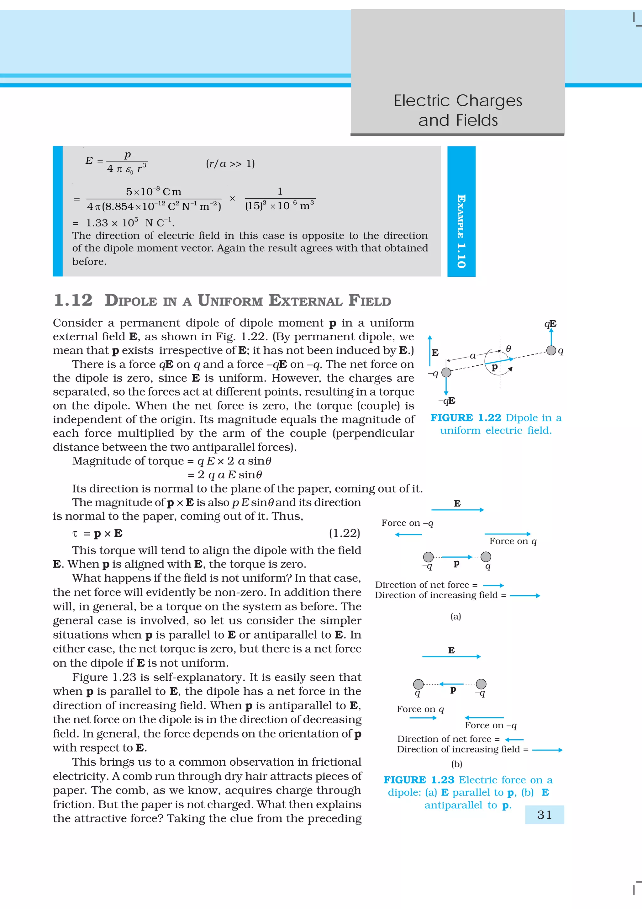
1.11 ELECTRIC DIPOLE
An electric dipole is a pair of equal and opposite point charges q and –q,
separated by a distance 2a. The line connecting the two charges defines
a direction in space. By convention, the direction from –q to q is said to
be the direction of the dipole. The mid-point of locations of –q and q is
called the centre of the dipole.
The total charge of the electric dipole is obviously zero. This does not
mean that the field of the electric dipole is zero. Since the charge q and
–q are separated by some distance, the electric fields due to them, when
added, do not exactly cancel out. However, at distances much larger than
the separation of the two charges forming a dipole (r >> 2a), the fields
due to q and –q nearly cancel out. The electric field due to a dipole
therefore falls off, at large distance, faster than like 1/r2
(the dependence
on r of the field due to a single charge q). These qualitative ideas are
borne out by the explicit calculation as follows:
1.11.1 The field of an electric dipole
The electric field of the pair of charges (–q and q) at any point in space
can be found out from Coulomb’s law and the superposition principle.
The results are simple for the following two cases: (i) when the point is on
the dipole axis, and (ii) when it is in the equatorial plane of the dipole,
i.e., on a plane perpendicular to the dipole axis through its centre. The
electric field at any general point P is obtained by adding the electric
fields E–q due to the charge –q and E+q due to the charge q, by the
parallelogram law of vectors.
(i) For points on the axis
Let the point P be at distance r from the centre of the dipole on the side of
the charge q, as shown in Fig. 1.20(a). Then
2
0
ˆ
4 ( )
q
q
r aε
− = −
π +
E p [1.13(a)]
where ˆp is the unit vector along the dipole axis (from –q to q). Also
2
0
ˆ
4 ( )
q
q
r aε
+ =
π −
E p [1.13(b)]

32. 28
Physics
The total field at P is
2 2
0
1 1
ˆ
4 ( ) ( )
q q
q
r a r aε+ −
⎡ ⎤
= + = −⎢ ⎥
π − +⎣ ⎦
E E E p
2 2 2
4
ˆ
4 ( )o
a rq
r aε
=
π −
p (1.14)
For r >> a
3
0
4
ˆ
4
q a
rε
=
π
E p (r >> a) (1.15)
(ii) For points on the equatorial plane
The magnitudes of the electric fields due to the two
charges +q and –q are given by
2 2
0
1
4
q
q
E
r aε+ =
π + [1.16(a)]
– 2 2
0
1
4
q
q
E
r aε
=
π +
[1.16(b)]
and are equal.
The directions of E+q and E–q are as shown in
Fig. 1.20(b). Clearly, the components normal to the dipole
axis cancel away. The components along the dipole axis
add up. The total electric field is opposite to ˆp. We have
E = – (E +q + E –q ) cosθ ˆp
2 2 3/2
2
ˆ
4 ( )o
q a
r aε
= −
π +
p (1.17)
At large distances (r >> a), this reduces to
3
2
ˆ ( )
4 o
q a
r a
rε
= − >>
π
E p (1.18)
From Eqs. (1.15) and (1.18), it is clear that the dipole field at large
distances does not involve q and a separately; it depends on the product
qa. This suggests the definition of dipole moment. The dipole moment
vector p of an electric dipole is defined by
p = q × 2a ˆp (1.19)
that is, it is a vector whose magnitude is charge q times the separation
2a (between the pair of charges q, –q) and the direction is along the line
from –q to q. In terms of p, the electric field of a dipole at large distances
takes simple forms:
At a point on the dipole axis
3
2
4 orε
=
π
p
E (r >> a) (1.20)
At a point on the equatorial plane
3
4 orε
= −
π
p
E (r >> a) (1.21)
FIGURE 1.20 Electric field of a dipole
at (a) a point on the axis, (b) a point
on the equatorial plane of the dipole.
p is the dipole moment vector of
magnitude p = q × 2a and
directed from –q to q.

33. Electric Charges
and Fields
29
EXAMPLE1.10
Notice the important point that the dipole field at large distances
falls off not as 1/r2
but as1/r3
. Further, the magnitude and the direction
of the dipole field depends not only on the distance r but also on the
angle between the position vector r and the dipole moment p.
We can think of the limit when the dipole size 2a approaches zero,
the charge q approaches infinity in such a way that the product
p = q × 2a is finite. Such a dipole is referred to as a point dipole. For a
point dipole, Eqs. (1.20) and (1.21) are exact, true for any r.
1.11.2 Physical significance of dipoles
In most molecules, the centres of positive charges and of negative charges*
lie at the same place. Therefore, their dipole moment is zero. CO2
and
CH4
are of this type of molecules. However, they develop a dipole moment
when an electric field is applied. But in some molecules, the centres of
negative charges and of positive charges do not coincide. Therefore they
have a permanent electric dipole moment, even in the absence of an electric
field. Such molecules are called polar molecules. Water molecules, H2O,
is an example of this type. Various materials give rise to interesting
properties and important applications in the presence or absence of
electric field.
Example 1.10 Two charges ±10 μC are placed 5.0 mm apart.
Determine the electric field at (a) a point P on the axis of the dipole
15 cm away from its centre O on the side of the positive charge, as
shown in Fig. 1.21(a), and (b) a point Q, 15 cm away from O on a line
passing through O and normal to the axis of the dipole, as shown in
Fig. 1.21(b).
FIGURE 1.21
* Centre of a collection of positive point charges is defined much the same way
as the centre of mass: cm
i ii
i
i
q
q
∑
=
∑
r
r .

34. 30
Physics
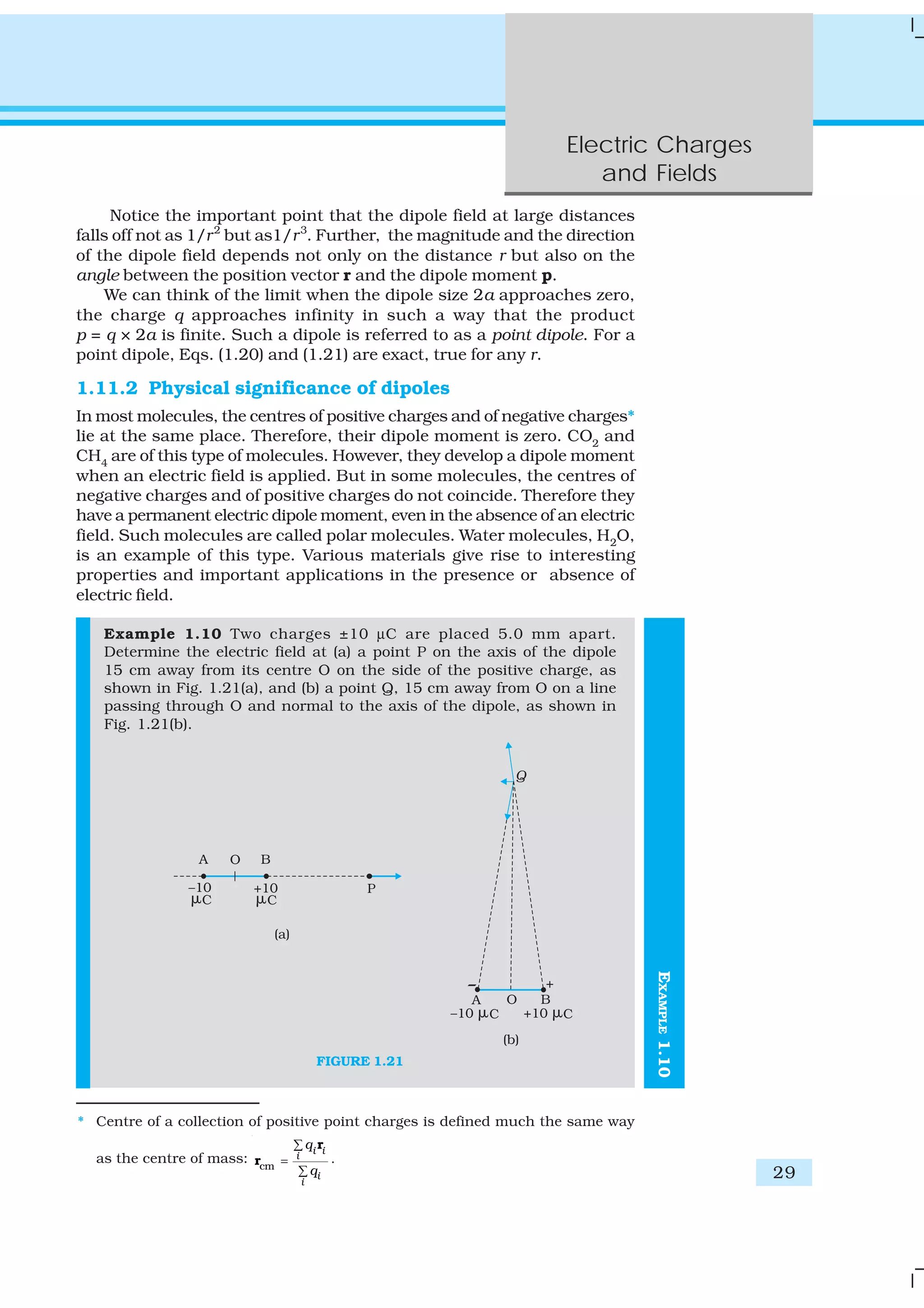
EXAMPLE1.10
Solution (a) Field at P due to charge +10 μC
=
5
12 2 1 2
10 C
4 (8.854 10 C N m )
−
− − −
π ×
2 4 2
1
(15 0.25) 10 m−
×
− ×
= 4.13 × 106
N C–1
along BP
Field at P due to charge –10 μC
–5
12 2 1 2
10 C
4 (8.854 10 C N m )− − −
=
π ×
2 4 2
1
(15 0.25) 10 m−
×
+ ×
= 3.86 × 106
N C–1
along PA
The resultant electric field at P due to the two charges at A and B is
= 2.7 × 105
N C–1
along BP.
In this example, the ratio OP/OB is quite large (= 60). Thus, we can
expect to get approximately the same result as above by directly using
the formula for electric field at a far-away point on the axis of a dipole.
For a dipole consisting of charges ± q, 2a distance apart, the electric
field at a distance r from the centre on the axis of the dipole has a
magnitude
3
0
2
4
p
E
rε
=
π
(r/a >> 1)
where p = 2a q is the magnitude of the dipole moment.
The direction of electric field on the dipole axis is always along the
direction of the dipole moment vector (i.e., from –q to q). Here,
p =10–5
C × 5 × 10–3
m = 5 × 10–8
C m
Therefore,
E =
8
12 2 1 2
2 5 10 C m
4 (8.854 10 C N m )
−
− − −
× ×
π ×
3 6 3
1
(15) 10 m−
×
×
= 2.6 × 105
N C–1
along the dipole moment direction AB, which is close to the result
obtained earlier.
(b) Field at Q due to charge + 10 μC at B
=
5
12 2 1 2
10 C
4 (8.854 10 C N m )
−
− − −
π × 2 2 4 2
1
[15 (0.25) ] 10 m−
+ ×
×
= 3.99 × 106
N C–1
along BQ
Field at Q due to charge –10 μC at A
=
5
12 2 1 2
10 C
4 (8.854 10 C N m )
−
− − −
π ×
2 2 4 2
1
[15 (0.25) ] 10 m−
+ ×
×
= 3.99 × 106
N C–1
along QA.
Clearly, the components of these two forces with equal magnitudes
cancel along the direction OQ but add up along the direction parallel
to BA. Therefore, the resultant electric field at Q due to the two
charges at A and B is
= 2 ×
6 –1
2 2
0.25
3.99 10 N C
15 (0.25)
× ×
+
along BA
= 1.33 × 105
N C–1
along BA.
As in (a), we can expect to get approximately the same result by
directly using the formula for dipole field at a point on the normal to
the axis of the dipole:

35. Electric Charges
and Fields
31
EXAMPLE1.10
3
4
p
E
rε0
=
π (r/a >> 1)
8
12 2 –1 –2
5 10 Cm
4 (8.854 10 C N m )
−
−
×
=
π ×
3 6 3
1
(15) 10 m−
×
×
= 1.33 × 105
N C–1
.
The direction of electric field in this case is opposite to the direction
of the dipole moment vector. Again the result agrees with that obtained
before.
1.12 DIPOLE IN A UNIFORM EXTERNAL FIELD
Consider a permanent dipole of dipole moment p in a uniform
external field E, as shown in Fig. 1.22. (By permanent dipole, we
mean that p exists irrespective of E; it has not been induced by E.)
There is a force qE on q and a force –qE on –q. The net force on
the dipole is zero, since E is uniform. However, the charges are
separated, so the forces act at different points, resulting in a torque
on the dipole. When the net force is zero, the torque (couple) is
independent of the origin. Its magnitude equals the magnitude of
each force multiplied by the arm of the couple (perpendicular
distance between the two antiparallel forces).
Magnitude of torque = q E × 2 a sinθ
= 2 q a E sinθ
Its direction is normal to the plane of the paper, coming out of it.
The magnitude of p × E is also p E sinθ and its direction
is normal to the paper, coming out of it. Thus,
τ = p × E (1.22)
This torque will tend to align the dipole with the field
E. When p is aligned with E, the torque is zero.
What happens if the field is not uniform? In that case,
the net force will evidently be non-zero. In addition there
will, in general, be a torque on the system as before. The
general case is involved, so let us consider the simpler
situations when p is parallel to E or antiparallel to E. In
either case, the net torque is zero, but there is a net force
on the dipole if E is not uniform.
Figure 1.23 is self-explanatory. It is easily seen that
when p is parallel to E, the dipole has a net force in the
direction of increasing field. When p is antiparallel to E,
the net force on the dipole is in the direction of decreasing
field. In general, the force depends on the orientation of p
with respect to E.
This brings us to a common observation in frictional
electricity. A comb run through dry hair attracts pieces of
paper. The comb, as we know, acquires charge through
friction. But the paper is not charged. What then explains
the attractive force? Taking the clue from the preceding
FIGURE 1.22 Dipole in a
uniform electric field.
FIGURE 1.23 Electric force on a
dipole: (a) E parallel to p, (b) E
antiparallel to p.

36. 32
Physics
discussion, the charged comb ‘polarizes’ the piece of paper, i.e., induces
a net dipole moment in the direction of field. Further, the electric field
due to the comb is not uniform. In this situation, it is easily seen that the
paper should move in the direction of the comb!
1.13 CONTINUOUS CHARGE DISTRIBUTION
We have so far dealt with charge configurations involving discrete charges
q1
, q2
, ..., qn
. One reason why we restricted to discrete charges is that the
mathematical treatment is simpler and does not involve calculus. For
many purposes, however, it is impractical to work in terms of discrete
charges and we need to work with continuous charge distributions. For
example, on the surface of a charged conductor, it is impractical to specify
the charge distribution in terms of the locations of the microscopic charged
constituents. It is more feasible to consider an area element ΔS (Fig. 1.24)
on the surface of the conductor (which is very small on the macroscopic
scale but big enough to include a very large number of electrons) and
specify the charge ΔQ on that element. We then define a surface charge
density σ at the area element by
Q
S
σ
Δ
=
Δ
(1.23)
We can do this at different points on the conductor and thus arrive at
a continuous function σ, called the surface charge density. The surface
charge density σ so defined ignores the quantisation of charge and the
discontinuity in charge distribution at the microscopic level*. σ represents
macroscopic surface charge density, which in a sense, is a smoothed out
average of the microscopic charge density over an area element ΔS which,
as said before, is large microscopically but small macroscopically. The
units for σ are C/m2
.
Similar considerations apply for a line charge distribution and a volume
charge distribution. The linear charge density λ of a wire is defined by
Q
l
λ
Δ
=
Δ
(1.24)
where Δl is a small line element of wire on the macroscopic scale that,
however, includes a large number of microscopic charged constituents,
and ΔQ is the charge contained in that line element. The units for λ are
C/m. The volume charge density (sometimes simply called charge density)
is defined in a similar manner:
Q
V
ρ
Δ
=
Δ
(1.25)
where ΔQ is the charge included in the macroscopically small volume
element ΔV that includes a large number of microscopic charged
constituents. The units for ρ are C/m3
.
The notion of continuous charge distribution is similar to that we
adopt for continuous mass distribution in mechanics. When we refer to
FIGURE 1.24
Definition of linear,
surface and volume
charge densities.
In each case, the
element (Δl, ΔS, ΔV)
chosen is small on
the macroscopic
scale but contains
a very large number
of microscopic
constituents.
* At the microscopic level, charge distribution is discontinuous, because they are
discrete charges separated by intervening space where there is no charge.

37. Electric Charges
and Fields
33
the density of a liquid, we are referring to its macroscopic density. We
regard it as a continuous fluid and ignore its discrete molecular
constitution.
The field due to a continuous charge distribution can be obtained in
much the same way as for a system of discrete charges, Eq. (1.10). Suppose
a continuous charge distribution in space has a charge density ρ. Choose
any convenient origin O and let the position vector of any point in the
charge distribution be r. The charge density ρ may vary from point to
point, i.e., it is a function of r. Divide the charge distribution into small
volume elements of size ΔV. The charge in a volume element ΔV is ρΔV.
Now, consider any general point P (inside or outside the distribution)
with position vector R (Fig. 1.24). Electric field due to the charge ρΔV is
given by Coulomb’s law:
2
0
1
ˆ
4
V
'
r'
ρ
ε
Δ
Δ =
π
E r (1.26)
where r′ is the distance between the charge element and P, and ˆr′ is a
unit vector in the direction from the charge element to P. By the
superposition principle, the total electric field due to the charge
distribution is obtained by summing over electric fields due to different
volume elements:
2
0
1
ˆ
4 all V
V
'
r'
ρ
ε Δ
Δ
≅ Σ
π
E r (1.27)
Note that ρ, r′, ˆ′r all can vary from point to point. In a strict
mathematical method, we should let ΔV→0 and the sum then becomes
an integral; but we omit that discussion here, for simplicity. In short,
using Coulomb’s law and the superposition principle, electric field can
be determined for any charge distribution, discrete or continuous or part
discrete and part continuous.
1.14 GAUSS’S LAW
As a simple application of the notion of electric flux, let us consider the
total flux through a sphere of radius r, which encloses a point charge q
at its centre. Divide the sphere into small area elements, as shown in
Fig. 1.25.
The flux through an area element ΔS is
2
0
ˆ
4
q
r
φ
ε
Δ = Δ = Δ
π
E S r Si i (1.28)
where we have used Coulomb’s law for the electric field due to a single
charge q. The unit vector ˆr is along the radius vector from the centre to
the area element. Now, since the normal to a sphere at every point is
along the radius vector at that point, the area element ΔS and ˆr have
the same direction. Therefore,
2
04
q
S
r
φ
ε
Δ = Δ
π (1.29)
since the magnitude of a unit vector is 1.
The total flux through the sphere is obtained by adding up flux
through all the different area elements:
FIGURE 1.25 Flux
through a sphere
enclosing a point
charge q at its centre.

38. 34
Physics
2
04all S
q
S
r
φ
εΔ
= Σ Δ
π
Since each area element of the sphere is at the same
distance r from the charge,
2 2
04 4all S
o
q q
S S
r r
φ
ε εΔ
= Σ Δ =
π π
Now S, the total area of the sphere, equals 4πr2
. Thus,
2
2
00
4
4
q q
r
r
φ
εε
= × π =
π (1.30)
Equation (1.30) is a simple illustration of a general result of
electrostatics called Gauss’s law.
We state Gauss’s law without proof:
Electric flux through a closed surface S
= q/ε0
(1.31)
q = total charge enclosed by S.
The law implies that the total electric flux through a closed surface is
zero if no charge is enclosed by the surface. We can see that explicitly in
the simple situation of Fig. 1.26.
Here the electric field is uniform and we are considering a closed
cylindrical surface, with its axis parallel to the uniform field E. The total
flux φ through the surface is φ = φ1
+ φ2
+ φ3
, where φ1
and φ2
represent
the flux through the surfaces 1 and 2 (of circular cross-section) of the
cylinder and φ3
is the flux through the curved cylindrical part of the
closed surface. Now the normal to the surface 3 at every point is
perpendicular to E, so by definition of flux, φ3 = 0. Further, the outward
normal to 2 is along E while the outward normal to 1 is opposite to E.
Therefore,
φ1
= –E S1
, φ2
= +E S2
S1
= S2
= S
where S is the area of circular cross-section. Thus, the total flux is zero,
as expected by Gauss’s law. Thus, whenever you find that the net electric
flux through a closed surface is zero, we conclude that the total charge
contained in the closed surface is zero.
The great significance of Gauss’s law Eq. (1.31), is that it is true in
general, and not only for the simple cases we have considered above. Let
us note some important points regarding this law:
(i) Gauss’s law is true for any closed surface, no matter what its shape
or size.
(ii) The term q on the right side of Gauss’s law, Eq. (1.31), includes the
sum of all charges enclosed by the surface. The charges may be located
anywhere inside the surface.
(iii) In the situation when the surface is so chosen that there are some
charges inside and some outside, the electric field [whose flux appears
on the left side of Eq. (1.31)] is due to all the charges, both inside and
outside S. The term q on the right side of Gauss’s law, however,
represents only the total charge inside S.
FIGURE 1.26 Calculation of the
flux of uniform electric field
through the surface of a cylinder.

39. Electric Charges
and Fields
35
EXAMPLE1.11
(iv) The surface that we choose for the application of Gauss’s law is called
the Gaussian surface. You may choose any Gaussian surface and
apply Gauss’s law. However, take care not to let the Gaussian surface
pass through any discrete charge. This is because electric field due
to a system of discrete charges is not well defined at the location of
any charge. (As you go close to the charge, the field grows without
any bound.) However, the Gaussian surface can pass through a
continuous charge distribution.
(v) Gauss’s law is often useful towards a much easier calculation of the
electrostatic field when the system has some symmetry. This is
facilitated by the choice of a suitable Gaussian surface.
(vi) Finally, Gauss’s law is based on the inverse square dependence on
distance contained in the Coulomb’s law. Any violation of Gauss’s
law will indicate departure from the inverse square law.
Example 1.11 The electric field components in Fig. 1.27 are
Ex
= αx1/2
, Ey
= Ez
= 0, in which α = 800 N/C m1/2
. Calculate (a) the
flux through the cube, and (b) the charge within the cube. Assume
that a = 0.1 m.
FIGURE 1.27
Solution
(a) Since the electric field has only an x component, for faces
perpendicular to x direction, the angle between E and ΔS is
± π/2. Therefore, the flux φ = E.ΔS is separately zero for each face
of the cube except the two shaded ones. Now the magnitude of
the electric field at the left face is
EL
= αx1/2
= αa1/2
(x = a at the left face).
The magnitude of electric field at the right face is
ER
= α x1/2
= α (2a)1/2
(x = 2a at the right face).
The corresponding fluxes are
φL
= EL
.ΔS = ˆL LSΔ E n⋅ =EL
ΔS cosθ = –EL
ΔS, since θ = 180°
= –EL
a2
φR
= ER
.ΔS = ER
ΔS cosθ = ER
ΔS, since θ = 0°
= ER
a2
Net flux through the cube

40. 36
Physics
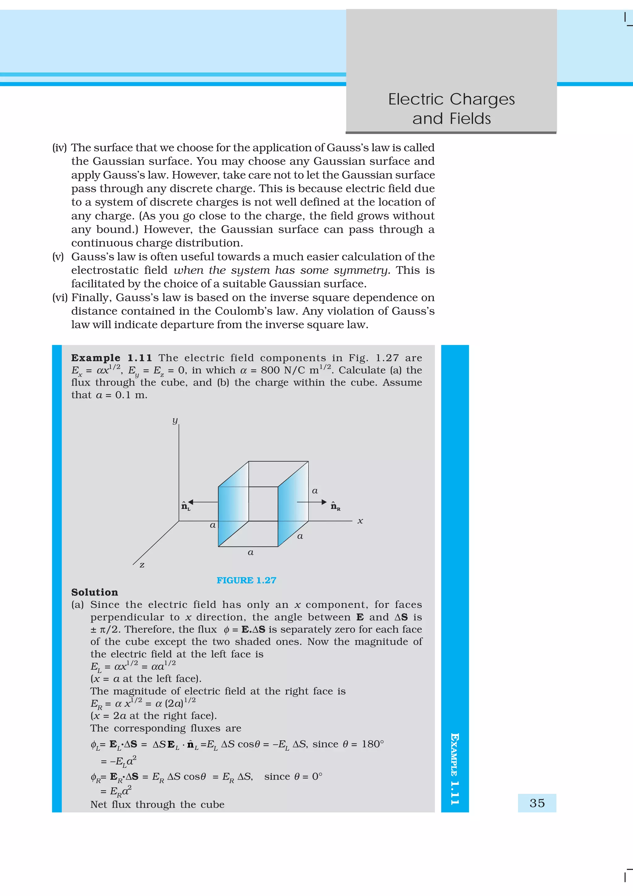
EXAMPLE1.12EXAMPLE1.11
= φR
+ φL
= ER
a2
– EL
a2
= a2
(ER
– EL
) = αa2
[(2a)1/2
– a1/2
]
= αa5/2
( )2 – 1
= 800 (0.1)5/2
( )2 – 1
= 1.05 N m2
C–1
(b) We can use Gauss’s law to find the total charge q inside the cube.
We have φ = q/ε0
or q = φε0
. Therefore,
q = 1.05 × 8.854 × 10–12
C = 9.27 × 10–12
C.
Example 1.12 An electric field is uniform, and in the positive x
direction for positive x, and uniform with the same magnitude but in
the negative x direction for negative x. It is given that E = 200 ˆi N/C
for x > 0 and E = –200 ˆi N/C for x < 0. A right circular cylinder of
length 20 cm and radius 5 cm has its centre at the origin and its axis
along the x-axis so that one face is at x = +10 cm and the other is at
x = –10 cm (Fig. 1.28). (a) What is the net outward flux through each
flat face? (b) What is the flux through the side of the cylinder?
(c) What is the net outward flux through the cylinder? (d) What is the
net charge inside the cylinder?
Solution
(a) We can see from the figure that on the left face E and ΔS are
parallel. Therefore, the outward flux is
φL
= E.ΔS = – 200 ˆ Δi Si
= + 200 ΔS, since ˆ Δi Si = – ΔS
= + 200 × π (0.05)2
= + 1.57 N m2
C–1
On the right face, E and ΔS are parallel and therefore
φR
= E.ΔS = + 1.57 N m2
C–1
.
(b) For any point on the side of the cylinder E is perpendicular to
ΔS and hence E.ΔS = 0. Therefore, the flux out of the side of the
cylinder is zero.
(c) Net outward flux through the cylinder
φ = 1.57 + 1.57 + 0 = 3.14 N m2
C–1
FIGURE 1.28
(d) The net charge within the cylinder can be found by using Gauss’s
law which gives
q = ε0
φ
= 3.14 × 8.854 × 10–12
C
= 2.78 × 10–11
C

41. Electric Charges
and Fields
37
1.15 APPLICATIONS OF GAUSS’S LAW
The electric field due to a general charge distribution is, as seen above,
given by Eq. (1.27). In practice, except for some special cases, the
summation (or integration) involved in this equation cannot be carried
out to give electric field at every point in
space. For some symmetric charge
configurations, however, it is possible to
obtain the electric field in a simple way using
the Gauss’s law. This is best understood by
some examples.
1.15.1 Field due to an infinitely
long straight uniformly
charged wire
Consider an infinitely long thin straight wire
with uniform linear charge density λ. The wire
is obviously an axis of symmetry. Suppose we
take the radial vector from O to P and rotate it
around the wire. The points P, P′, P′′ so
obtained are completely equivalent with
respect to the charged wire. This implies that
the electric field must have the same magnitude
at these points. The direction of electric field at
every point must be radial (outward if λ > 0,
inward if λ < 0). This is clear from Fig. 1.29.
Consider a pair of line elements P1
and P2
of the wire, as shown. The electric fields
produced by the two elements of the pair when
summed give a resultant electric field which
is radial (the components normal to the radial
vector cancel). This is true for any such pair
and hence the total field at any point P is
radial. Finally, since the wire is infinite,
electric field does not depend on the position
of P along the length of the wire. In short, the
electric field is everywhere radial in the plane
cutting the wire normally, and its magnitude
depends only on the radial distance r.
To calculate the field, imagine a cylindrical
Gaussian surface, as shown in the Fig. 1.29(b).
Since the field is everywhere radial, flux
through the two ends of the cylindrical
Gaussian surface is zero. At the cylindrical
part of the surface, E is normal to the surface
at every point, and its magnitude is constant,
since it depends only on r. The surface area
of the curved part is 2πrl, where l is the length
of the cylinder.
FIGURE 1.29 (a) Electric field due to an
infinitely long thin straight wire is radial,
(b) The Gaussian surface for a long thin
wire of uniform linear charge density.

42. 38
Physics
Flux through the Gaussian surface
= flux through the curved cylindrical part of the surface
= E × 2πrl
The surface includes charge equal to λ l. Gauss’s law then gives
E × 2πrl = λl/ε0
i.e., E =
02 r
λ
επ
Vectorially, E at any point is given by
0
ˆ
2 r
λ
ε
=
π
E n (1.32)
where ˆn is the radial unit vector in the plane normal to the wire passing
through the point. E is directed outward if λ is positive and inward if λ is
negative.
Note that when we write a vector A as a scalar multiplied by a unit
vector, i.e., as A = A ˆa , the scalar A is an algebraic number. It can be
negative or positive. The direction of A will be the same as that of the unit
vector ˆa if A > 0 and opposite to ˆa if A < 0. When we want to restrict to
non-negative values, we use the symbol A and call it the modulus of A.
Thus, 0≥A .
Also note that though only the charge enclosed by the surface (λl)
was included above, the electric field E is due to the charge on the entire
wire. Further, the assumption that the wire is infinitely long is crucial.
Without this assumption, we cannot take E to be normal to the curved
part of the cylindrical Gaussian surface. However, Eq. (1.32) is
approximately true for electric field around the central portions of a long
wire, where the end effects may be ignored.
1.15.2 Field due to a uniformly charged infinite plane sheet
Let σ be the uniform surface charge density of an infinite plane sheet
(Fig. 1.30). We take the x-axis normal to the given plane. By symmetry,
the electric field will not depend on y and z coordinates and its direction
at every point must be parallel to the x-direction.
We can take the Gaussian surface to be a
rectangular parallelepiped of cross sectional area
A, as shown. (A cylindrical surface will also do.) As
seen from the figure, only the two faces 1 and 2 will
contribute to the flux; electric field lines are parallel
to the other faces and they, therefore, do not
contribute to the total flux.
The unit vector normal to surface 1 is in –x
direction while the unit vector normal to surface 2
is in the +x direction. Therefore, flux E.ΔS through
both the surfaces are equal and add up. Therefore
the net flux through the Gaussian surface is 2 EA.
The charge enclosed by the closed surface is σA.
Therefore by Gauss’s law,
FIGURE 1.30 Gaussian surface for a
uniformly charged infinite plane sheet.

43. Electric Charges
and Fields
39
2 EA = σA/ε0
or, E = σ/2ε0
Vectorically,
0
ˆ
2
σ
ε
=E n (1.33)
where ˆn is a unit vector normal to the plane and going away from it.
E is directed away from the plate if σ is positive and toward the plate
if σ is negative. Note that the above application of the Gauss’ law has
brought out an additional fact: E is independent of x also.
For a finite large planar sheet, Eq. (1.33) is approximately true in the
middle regions of the planar sheet, away from the ends.
1.15.3 Field due to a uniformly charged thin spherical shell
Let σ be the uniform surface charge density of a thin spherical shell of
radius R (Fig. 1.31). The situation has obvious spherical symmetry. The
field at any point P, outside or inside, can depend only on r (the radial
distance from the centre of the shell to the point) and must be radial (i.e.,
along the radius vector).
(i) Field outside the shell: Consider a point P outside the
shell with radius vector r. To calculate E at P, we take the
Gaussian surface to be a sphere of radius r and with centre
O, passing through P. All points on this sphere are equivalent
relative to the given charged configuration. (That is what we
mean by spherical symmetry.) The electric field at each point
of the Gaussian surface, therefore, has the same magnitude
E and is along the radius vector at each point. Thus, E and
ΔS at every point are parallel and the flux through each
element is E ΔS. Summing over all ΔS, the flux through the
Gaussian surface is E × 4 π r2
. The charge enclosed is
σ × 4 π R2
. By Gauss’s law
E × 4 π r2
=
2
0
4 R
σ
ε
π
Or,
2
2 2
0 04
R q
E
r r
σ
ε ε
= =
π
where q = 4 π R2
σ is the total charge on the spherical shell.
Vectorially,
2
0
ˆ
4
q
rε
=
π
E r (1.34)
The electric field is directed outward if q > 0 and inward if
q < 0. This, however, is exactly the field produced by a charge
q placed at the centre O. Thus for points outside the shell, the field due
to a uniformly charged shell is as if the entire charge of the shell is
concentrated at its centre.
(ii) Field inside the shell: In Fig. 1.31(b), the point P is inside the
shell. The Gaussian surface is again a sphere through P centred at O.
FIGURE 1.31 Gaussian
surfaces for a point with
(a) r > R, (b) r < R.

44. 40
Physics
EXAMPLE1.13
The flux through the Gaussian surface, calculated as before, is
E × 4 π r2
. However, in this case, the Gaussian surface encloses no
charge. Gauss’s law then gives
E × 4 π r2
= 0
i.e., E = 0 (r < R ) (1.35)
that is, the field due to a uniformly charged thin shell is zero at all points
inside the shell*. This important result is a direct consequence of Gauss’s
law which follows from Coulomb’s law. The experimental verification of
this result confirms the 1/r2
dependence in Coulomb’s law.
Example 1.13 An early model for an atom considered it to have a
positively charged point nucleus of charge Ze, surrounded by a
uniform density of negative charge up to a radius R. The atom as a
whole is neutral. For this model, what is the electric field at a distance
r from the nucleus?
FIGURE 1.32
Solution The charge distribution for this model of the atom is as
shown in Fig. 1.32. The total negative charge in the uniform spherical
charge distribution of radius R must be –Z e, since the atom (nucleus
of charge Z e + negative charge) is neutral. This immediately gives us
the negative charge density ρ, since we must have
3
4
0–
3
R
Zeρ
π
=
or 3
3
4
Ze
R
ρ = −
π
To find the electric field E(r) at a point P which is a distance r away
from the nucleus, we use Gauss’s law. Because of the spherical
symmetry of the charge distribution, the magnitude of the electric
field E(r) depends only on the radial distance, no matter what the
direction of r. Its direction is along (or opposite to) the radius vector r
from the origin to the point P. The obvious Gaussian surface is a
spherical surface centred at the nucleus. We consider two situations,
namely, r < R and r > R.
(i) r < R : The electric flux φ enclosed by the spherical surface is
φ = E (r) × 4 π r2
where E (r) is the magnitude of the electric field at r. This is because
* Compare this with a uniform mass shell discussed in Section 8.5 of Class XI
Textbook of Physics.

45. Electric Charges
and Fields
41
EXAMPLE1.13
the field at any point on the spherical Gaussian surface has the
same direction as the normal to the surface there, and has the same
magnitude at all points on the surface.
The charge q enclosed by the Gaussian surface is the positive nuclear
charge and the negative charge within the sphere of radius r,
i.e.,
3
4
3
r
q Z e ρ
π
= +
Substituting for the charge density ρ obtained earlier, we have
3
3
r
q Z e Z e
R
= −
Gauss’s law then gives,
2 3
0
1
( ) ;
4
Z e r
E r r R
r Rε
⎛ ⎞
= − <⎜ ⎟⎝ ⎠π
The electric field is directed radially outward.
(ii) r > R: In this case, the total charge enclosed by the Gaussian
spherical surface is zero since the atom is neutral. Thus, from Gauss’s
law,
E (r) × 4 π r2
= 0 or E (r) = 0; r > R
At r = R, both cases give the same result: E = 0.
ON SYMMETRY OPERATIONS
In Physics, we often encounter systems with various symmetries. Consideration of these
symmetries helps one arrive at results much faster than otherwise by a straightforward
calculation. Consider, for example an infinite uniform sheet of charge (surface charge
density σ) along the y-z plane. This system is unchanged if (a) translated parallel to the
y-z plane in any direction, (b) rotated about the x-axis through any angle. As the system
is unchanged under such symmetry operation, so must its properties be. In particular,
in this example, the electric field E must be unchanged.
Translation symmetry along the y-axis shows that the electric field must be the same
at a point (0, y1
, 0) as at (0, y2
, 0). Similarly translational symmetry along the z-axis
shows that the electric field at two point (0, 0, z1
) and (0, 0, z2
) must be the same. By
using rotation symmetry around the x-axis, we can conclude that E must be
perpendicular to the y-z plane, that is, it must be parallel to the x-direction.
Try to think of a symmetry now which will tell you that the magnitude of the electric
field is a constant, independent of the x-coordinate. It thus turns out that the magnitude
of the electric field due to a uniformly charged infinite conducting sheet is the same at all
points in space. The direction, however, is opposite of each other on either side of the
sheet.
Compare this with the effort needed to arrive at this result by a direct calculation
using Coulomb’s law.

46. 42
Physics
SUMMARY
1. Electric and magnetic forces determine the properties of atoms,
molecules and bulk matter.
2. From simple experiments on frictional electricity, one can infer that
there are two types of charges in nature; and that like charges repel
and unlike charges attract. By convention, the charge on a glass rod
rubbed with silk is positive; that on a plastic rod rubbed with fur is
then negative.
3. Conductors allow movement of electric charge through them, insulators
do not. In metals, the mobile charges are electrons; in electrolytes
both positive and negative ions are mobile.
4. Electric charge has three basic properties: quantisation, additivity
and conservation.
Quantisation of electric charge means that total charge (q) of a body
is always an integral multiple of a basic quantum of charge (e) i.e.,
q = n e, where n = 0, ±1, ±2, ±3, .... Proton and electron have charges
+e, –e, respectively. For macroscopic charges for which n is a very large
number, quantisation of charge can be ignored.
Additivity of electric charges means that the total charge of a system
is the algebraic sum (i.e., the sum taking into account proper signs)
of all individual charges in the system.
Conservation of electric charges means that the total charge of an
isolated system remains unchanged with time. This means that when
bodies are charged through friction, there is a transfer of electric charge
from one body to another, but no creation or destruction of charge.
5. Coulomb’s Law: The mutual electrostatic force between two point
charges q1 and q2 is proportional to the product q1q2 and inversely
proportional to the square of the distance r21
separating them.
Mathematically,
F21
= force on q2
due to
1 2
1 212
21
ˆ
k (q q )
q
r
= r
where 21
ˆr is a unit vector in the direction from q1 to q2 and k =
0
1
4 επ
is the constant of proportionality.
In SI units, the unit of charge is coulomb. The experimental value of
the constant ε0
is
ε0 = 8.854 × 10–12
C2
N–1
m–2
The approximate value of k is
k = 9 × 109
N m2
C–2
6. The ratio of electric force and gravitational force between a proton
and an electron is
2
39
2 4 10
e p
k e
.
G m m
≅ ×
7. Superposition Principle: The principle is based on the property that the
forces with which two charges attract or repel each other are not
affected by the presence of a third (or more) additional charge(s). For
an assembly of charges q1, q2, q3, ..., the force on any charge, say q1, is

47. Electric Charges
and Fields
43
the vector sum of the force on q1
due to q2
, the force on q1
due to q3
,
and so on. For each pair, the force is given by the Coulomb’s law for
two charges stated earlier.
8. The electric field E at a point due to a charge configuration is the
force on a small positive test charge q placed at the point divided by
the magnitude of the charge. Electric field due to a point charge q has
a magnitude |q|/4πε0
r2
; it is radially outwards from q, if q is positive,
and radially inwards if q is negative. Like Coulomb force, electric field
also satisfies superposition principle.
9. An electric field line is a curve drawn in such a way that the tangent
at each point on the curve gives the direction of electric field at that
point. The relative closeness of field lines indicates the relative strength
of electric field at different points; they crowd near each other in regions
of strong electric field and are far apart where the electric field is
weak. In regions of constant electric field, the field lines are uniformly
spaced parallel straight lines.
10. Some of the important properties of field lines are: (i) Field lines are
continuous curves without any breaks. (ii) Two field lines cannot cross
each other. (iii) Electrostatic field lines start at positive charges and
end at negative charges —they cannot form closed loops.
11. An electric dipole is a pair of equal and opposite charges q and –q
separated by some distance 2a. Its dipole moment vector p has
magnitude 2qa and is in the direction of the dipole axis from –q to q.
12. Field of an electric dipole in its equatorial plane (i.e., the plane
perpendicular to its axis and passing through its centre) at a distance
r from the centre:
2 2 3/2
1
4 ( )o a rε
−
=
π +
p
E
3
,
4 o
for r a
rε
−
≅ >>
π
p
Dipole electric field on the axis at a distance r from the centre:
2 2 2
0
2
4 ( )
r
r aε
=
π −
p
E
3
0
2
4
for r a
rε
≅ >>
π
p
The 1/r3
dependence of dipole electric fields should be noted in contrast
to the 1/r2
dependence of electric field due to a point charge.
13. In a uniform electric field E, a dipole experiences a torque τ given by
τ = p × E
but experiences no net force.
14. The flux Δφ of electric field E through a small area element ΔS is
given by
Δφ = E.ΔS
The vector area element ΔS is
ΔS = ΔS ˆn
where ΔS is the magnitude of the area element and ˆn is normal to the
area element, which can be considered planar for sufficiently small ΔS.

48. 44
Physics
For an area element of a closed surface, ˆn is taken to be the direction
of outward normal, by convention.
15. Gauss’s law: The flux of electric field through any closed surface S is
1/ε0
times the total charge enclosed by S. The law is especially useful
in determining electric field E, when the source distribution has simple
symmetry:
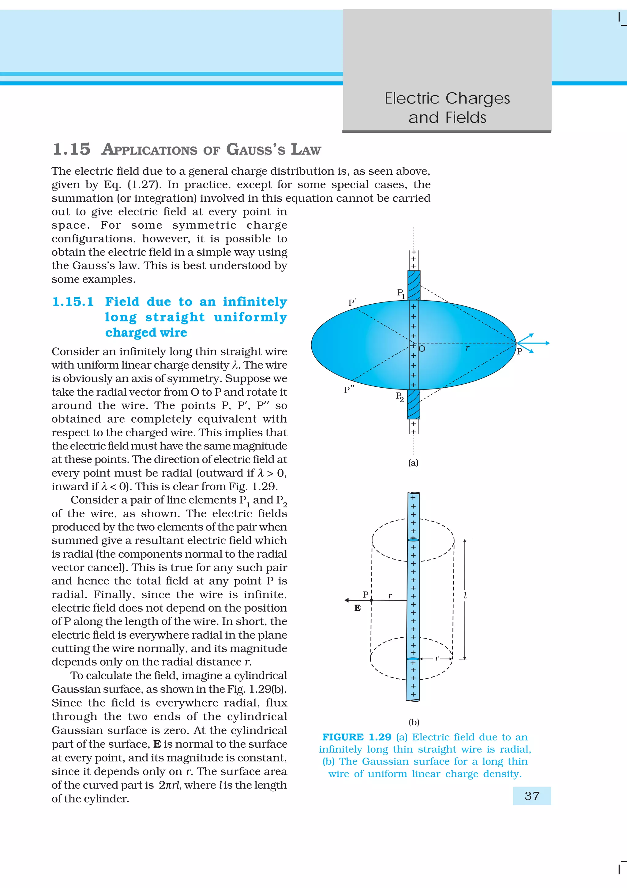
(i) Thin infinitely long straight wire of uniform linear charge density λ
0
ˆ
2 r
λ
ε
=
π
E n
where r is the perpendicular distance of the point from the wire and
ˆn is the radial unit vector in the plane normal to the wire passing
through the point.
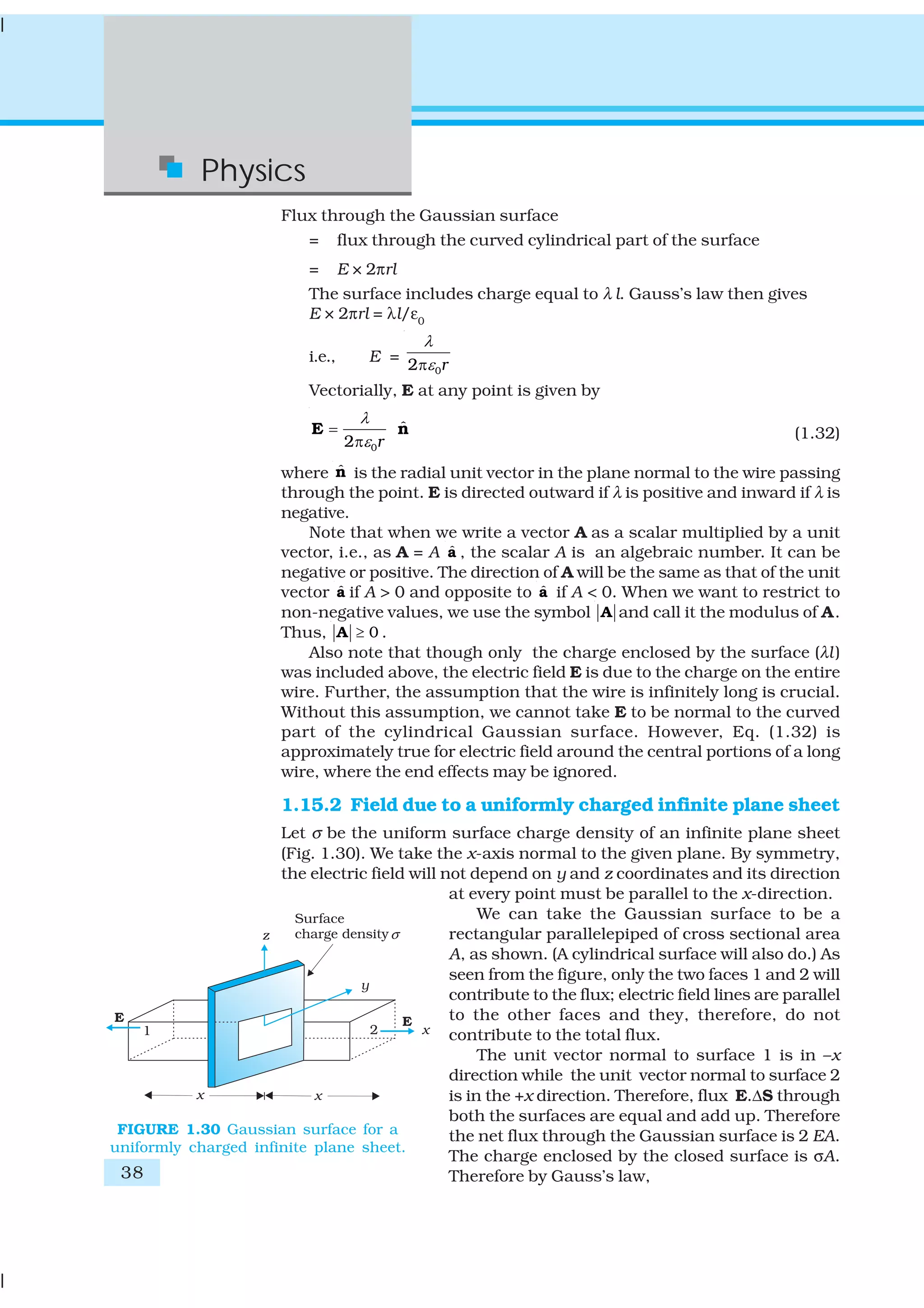
(ii) Infinite thin plane sheet of uniform surface charge density σ
0
ˆ
2
σ
ε
=E n
where ˆn is a unit vector normal to the plane, outward on either side.
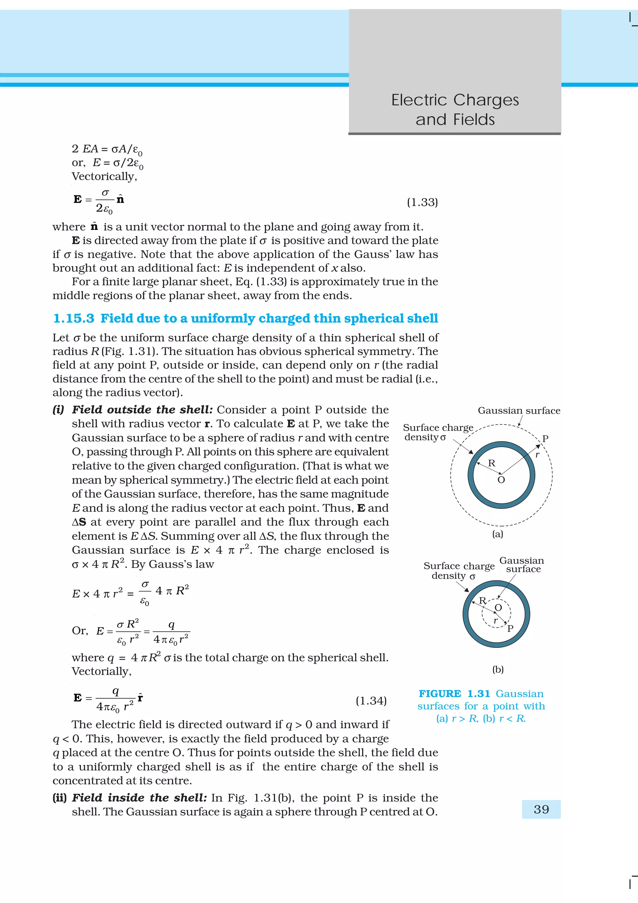
(iii) Thin spherical shell of uniform surface charge density σ
2
0
ˆ ( )
4
q
r R
rε
= ≥
π
E r
E = 0 (r < R)
where r is the distance of the point from the centre of the shell and R
the radius of the shell. q is the total charge of the shell: q = 4πR2
σ.
The electric field outside the shell is as though the total charge is
concentrated at the centre. The same result is true for a solid sphere
of uniform volume charge density. The field is zero at all points inside
the shell
Physical quantity Symbol Dimensions Unit Remarks
Vector area element Δ S [L2
] m2
ΔS = ΔS ˆn
Electric field E [MLT–3
A–1
] V m–1
Electric flux φ [ML3
T–3
A–1
] V m Δφ = E.ΔS
Dipole moment p [LTA] C m Vector directed
from negative to
positive charge
Charge density
linear λ [L–1
TA] C m–1
Charge/length
surface σ [L–2
TA] C m–2
Charge/area
volume ρ [L–3
TA] C m–3
Charge/volume

49. Electric Charges
and Fields
45
POINTS TO PONDER
1. You might wonder why the protons, all carrying positive charges, are
compactly residing inside the nucleus. Why do they not fly away? You
will learn that there is a third kind of a fundamental force, called the
strong force which holds them together. The range of distance where
this force is effective is, however, very small ~10-14
m. This is precisely
the size of the nucleus. Also the electrons are not allowed to sit on
top of the protons, i.e. inside the nucleus, due to the laws of quantum
mechanics. This gives the atoms their structure as they exist in nature.
2. Coulomb force and gravitational force follow the same inverse-square
law. But gravitational force has only one sign (always attractive), while
Coulomb force can be of both signs (attractive and repulsive), allowing
possibility of cancellation of electric forces. This is how gravity, despite
being a much weaker force, can be a dominating and more pervasive
force in nature.
3. The constant of proportionality k in Coulomb’s law is a matter of
choice if the unit of charge is to be defined using Coulomb’s law. In SI
units, however, what is defined is the unit of current (A) via its magnetic
effect (Ampere’s law) and the unit of charge (coulomb) is simply defined
by (1C = 1 A s). In this case, the value of k is no longer arbitrary; it is
approximately 9 × 109
N m2
C–2
.
4. The rather large value of k, i.e., the large size of the unit of charge
(1C) from the point of view of electric effects arises because (as
mentioned in point 3 already) the unit of charge is defined in terms of
magnetic forces (forces on current–carrying wires) which are generally
much weaker than the electric forces. Thus while 1 ampere is a unit
of reasonable size for magnetic effects, 1 C = 1 A s, is too big a unit for
electric effects.
5. The additive property of charge is not an ‘obvious’ property. It is related
to the fact that electric charge has no direction associated with it;
charge is a scalar.
6. Charge is not only a scalar (or invariant) under rotation; it is also
invariant for frames of reference in relative motion. This is not always
true for every scalar. For example, kinetic energy is a scalar under
rotation, but is not invariant for frames of reference in relative
motion.
7. Conservation of total charge of an isolated system is a property
independent of the scalar nature of charge noted in point 6.
Conservation refers to invariance in time in a given frame of reference.
A quantity may be scalar but not conserved (like kinetic energy in an
inelastic collision). On the other hand, one can have conserved vector
quantity (e.g., angular momentum of an isolated system).
8. Quantisation of electric charge is a basic (unexplained) law of nature;
interestingly, there is no analogous law on quantisation of mass.
9. Superposition principle should not be regarded as ‘obvious’, or equated
with the law of addition of vectors. It says two things: force on one
charge due to another charge is unaffected by the presence of other
charges, and there are no additional three-body, four-body, etc., forces
which arise only when there are more than two charges.
10. The electric field due to a discrete charge configuration is not defined
at the locations of the discrete charges. For continuous volume charge
distribution, it is defined at any point in the distribution. For a surface
charge distribution, electric field is discontinuous across the surface.

50. 46
Physics
11. The electric field due to a charge configuration with total charge zero
is not zero; but for distances large compared to the size of
the configuration, its field falls off faster than 1/r2
, typical of field
due to a single charge. An electric dipole is the simplest example of
this fact.
EXERCISES
1.1 What is the force between two small charged spheres having
charges of 2 × 10–7
C and 3 × 10–7
C placed 30 cm apart in air?
1.2 The electrostatic force on a small sphere of charge 0.4 μC due to
another small sphere of charge –0.8 μC in air is 0.2 N. (a) What is
the distance between the two spheres? (b) What is the force on the
second sphere due to the first?
1.3 Check that the ratio ke2
/G me
mp
is dimensionless. Look up a Table
of Physical Constants and determine the value of this ratio. What
does the ratio signify?
1.4 (a) Explain the meaning of the statement ‘electric charge of a body
is quantised’.
(b) Why can one ignore quantisation of electric charge when dealing
with macroscopic i.e., large scale charges?
1.5 When a glass rod is rubbed with a silk cloth, charges appear on
both. A similar phenomenon is observed with many other pairs of
bodies. Explain how this observation is consistent with the law of
conservation of charge.
1.6 Four point charges qA
= 2 μC, qB
= –5 μC, qC
= 2 μC, and qD
= –5 μC are
located at the corners of a square ABCD of side 10 cm. What is the
force on a charge of 1 μC placed at the centre of the square?
1.7 (a) An electrostatic field line is a continuous curve. That is, a field
line cannot have sudden breaks. Why not?
(b) Explain why two field lines never cross each other at any point?
1.8 Two point charges qA
= 3 μC and qB
= –3 μC are located 20 cm apart
in vacuum.
(a) What is the electric field at the midpoint O of the line AB joining
the two charges?
(b) If a negative test charge of magnitude 1.5 × 10–9
C is placed at
this point, what is the force experienced by the test charge?
1.9 A system has two charges qA
= 2.5 × 10–7
C and qB
= –2.5 × 10–7
C
located at points A: (0, 0, –15 cm) and B: (0,0, +15 cm), respectively.
What are the total charge and electric dipole moment of the system?
1.10 An electric dipole with dipole moment 4 × 10–9
C m is aligned at 30°
with the direction of a uniform electric field of magnitude 5 × 104
NC–1
.
Calculate the magnitude of the torque acting on the dipole.
1.11 A polythene piece rubbed with wool is found to have a negative
charge of 3 × 10–7
C.
(a) Estimate the number of electrons transferred (from which to
which?)
(b) Is there a transfer of mass from wool to polythene?
1.12 (a) Two insulated charged copper spheres A and B have their centres
separated by a distance of 50 cm. What is the mutual force of

51. Electric Charges
and Fields
47
electrostatic repulsion if the charge on each is 6.5 × 10–7
C? The
radii of A and B are negligible compared to the distance of
separation.
(b) What is the force of repulsion if each sphere is charged double
the above amount, and the distance between them is halved?
1.13 Suppose the spheres A and B in Exercise 1.12 have identical sizes.
A third sphere of the same size but uncharged is brought in contact
with the first, then brought in contact with the second, and finally
removed from both. What is the new force of repulsion between A
and B?
1.14 Figure 1.33 shows tracks of three charged particles in a uniform
electrostatic field. Give the signs of the three charges. Which particle
has the highest charge to mass ratio?
FIGURE 1.33
1.15 Consider a uniform electric field E = 3 × 103
î N/C. (a) What is the
flux of this field through a square of 10 cm on a side whose plane is
parallel to the yz plane? (b) What is the flux through the same
square if the normal to its plane makes a 60° angle with the x-axis?
1.16 What is the net flux of the uniform electric field of Exercise 1.15
through a cube of side 20 cm oriented so that its faces are parallel
to the coordinate planes?
1.17 Careful measurement of the electric field at the surface of a black
box indicates that the net outward flux through the surface of the
box is 8.0 × 103
Nm2
/C. (a) What is the net charge inside the box?
(b) If the net outward flux through the surface of the box were zero,
could you conclude that there were no charges inside the box? Why
or Why not?
1.18 A point charge +10 μC is a distance 5 cm directly above the centre
of a square of side 10 cm, as shown in Fig. 1.34. What is the
magnitude of the electric flux through the square? (Hint: Think of
the square as one face of a cube with edge 10 cm.)
FIGURE 1.34

52. 48
Physics
1.19 A point charge of 2.0 μC is at the centre of a cubic Gaussian
surface 9.0 cm on edge. What is the net electric flux through the
surface?
1.20 A point charge causes an electric flux of –1.0 × 103
Nm2
/C to pass
through a spherical Gaussian surface of 10.0 cm radius centred on
the charge. (a) If the radius of the Gaussian surface were doubled,
how much flux would pass through the surface? (b) What is the
value of the point charge?
1.21 A conducting sphere of radius 10 cm has an unknown charge. If
the electric field 20 cm from the centre of the sphere is 1.5 × 103
N/C
and points radially inward, what is the net charge on the sphere?
1.22 A uniformly charged conducting sphere of 2.4 m diameter has a
surface charge density of 80.0 μC/m2
. (a) Find the charge on the
sphere. (b) What is the total electric flux leaving the surface of the
sphere?
1.23 An infinite line charge produces a field of 9 × 104
N/C at a distance
of 2 cm. Calculate the linear charge density.
1.24 Two large, thin metal plates are parallel and close to each other. On
their inner faces, the plates have surface charge densities of opposite
signs and of magnitude 17.0 × 10–22
C/m2
. What is E: (a) in the outer
region of the first plate, (b) in the outer region of the second plate,
and (c) between the plates?
ADDITIONAL EXERCISES
1.25 An oil drop of 12 excess electrons is held stationary under a constant
electric field of 2.55 × 104
NC–1
in Millikan’s oil drop experiment. The
density of the oil is 1.26 g cm–3
. Estimate the radius of the drop.
(g = 9.81 m s–2
; e = 1.60 × 10–19
C).
1.26 Which among the curves shown in Fig. 1.35 cannot possibly
represent electrostatic field lines?

53. Electric Charges
and Fields
49
FIGURE 1.35
1.27 In a certain region of space, electric field is along the z-direction
throughout. The magnitude of electric field is, however, not constant
but increases uniformly along the positive z-direction, at the rate of
105
NC–1
per metre. What are the force and torque experienced by a
system having a total dipole moment equal to 10–7
Cm in the negative
z-direction ?
1.28 (a) A conductor A with a cavity as shown in Fig. 1.36(a) is given a
charge Q. Show that the entire charge must appear on the outer
surface of the conductor. (b) Another conductor B with charge q is
inserted into the cavity keeping B insulated from A. Show that the
total charge on the outside surface of A is Q + q [Fig. 1.36(b)]. (c) A
sensitive instrument is to be shielded from the strong electrostatic
fields in its environment. Suggest a possible way.
FIGURE 1.36
1.29 A hollow charged conductor has a tiny hole cut into its surface.
Show that the electric field in the hole is (σ/2ε0
) ˆn , where ˆn is the
unit vector in the outward normal direction, and σ is the surface
charge density near the hole.
1.30 Obtain the formula for the electric field due to a long thin wire of
uniform linear charge density λ without using Gauss’s law. [Hint:
Use Coulomb’s law directly and evaluate the necessary integral.]
1.31 It is now believed that protons and neutrons (which constitute nuclei
of ordinary matter) are themselves built out of more elementary units
called quarks. A proton and a neutron consist of three quarks each.
Two types of quarks, the so called ‘up’ quark (denoted by u) of charge
+ (2/3) e, and the ‘down’ quark (denoted by d) of charge (–1/3) e,
together with electrons build up ordinary matter. (Quarks of other
types have also been found which give rise to different unusual
varieties of matter.) Suggest a possible quark composition of a
proton and neutron.

54. 50
Physics
1.32 (a) Consider an arbitrary electrostatic field configuration. A small
test charge is placed at a null point (i.e., where E = 0) of the
configuration. Show that the equilibrium of the test charge is
necessarily unstable.
(b) Verify this result for the simple configuration of two charges of
the same magnitude and sign placed a certain distance apart.
1.33 A particle of mass m and charge (–q) enters the region between the
two charged plates initially moving along x-axis with speed vx
(like
particle 1 in Fig. 1.33). The length of plate is L and an uniform
electric field E is maintained between the plates. Show that the
vertical deflection of the particle at the far edge of the plate is
qEL2
/(2m vx
2
).
Compare this motion with motion of a projectile in gravitational field
discussed in Section 4.10 of Class XI Textbook of Physics.
1.34 Suppose that the particle in Exercise in 1.33 is an electron projected
with velocity vx
= 2.0 × 106
m s–1
. If E between the plates separated
by 0.5 cm is 9.1 × 102
N/C, where will the electron strike the upper
plate? (|e|=1.6 × 10–19
C, me
= 9.1 × 10–31
kg.)

55. 2.1 INTRODUCTION
In Chapters 6 and 8 (Class XI), the notion of potential energy was
introduced. When an external force does work in taking a body from a
point to another against a force like spring force or gravitational force,
that work gets stored as potential energy of the body. When the external
force is removed, the body moves, gaining kinetic energy and losing
an equal amount of potential energy. The sum of kinetic and
potential energies is thus conserved. Forces of this kind are called
conservative forces. Spring force and gravitational force are examples of
conservative forces.
Coulomb force between two (stationary) charges, like the gravitational
force, is also a conservative force. This is not surprising, since both have
inverse-square dependence on distance and differ mainly in the
proportionality constants – the masses in the gravitational law are
replaced by charges in Coulomb’s law. Thus, like the potential energy of
a mass in a gravitational field, we can define electrostatic potential energy
of a charge in an electrostatic field.
Consider an electrostatic field E due to some charge configuration.
First, for simplicity, consider the field E due to a charge Q placed at the
origin. Now, imagine that we bring a test charge q from a point R to a
point P against the repulsive force on it due to the charge Q. With reference
Chapter Two
ELECTROSTATIC
POTENTIAL AND
CAPACITANCE

56. Physics
52
to Fig. 2.1, this will happen if Q and q are both positive
or both negative. For definiteness, let us take Q, q > 0.
Two remarks may be made here. First, we assume
that the test charge q is so small that it does not disturb
the original configuration, namely the charge Q at the
origin (or else, we keep Q fixed at the origin by some
unspecified force). Second, in bringing the charge q from
R to P, we apply an external force Fext
just enough to
counter the repulsive electric force FE (i.e, Fext= –FE).
This means there is no net force on or acceleration of
the charge q when it is brought from R to P, i.e., it is
brought with infinitesimally slow constant speed. In
this situation, work done by the external force is the negative of the work
done by the electric force, and gets fully stored in the form of potential
energy of the charge q. If the external force is removed on reaching P, the
electric force will take the charge away from Q – the stored energy (potential
energy) at P is used to provide kinetic energy to the charge q in such a
way that the sum of the kinetic and potential energies is conserved.
Thus, work done by external forces in moving a charge q from R to P is
WRP
=
P
R
dext∫F rC
=
P
R
dE−∫F rC (2.1)
This work done is against electrostatic repulsive force and gets stored
as potential energy.
At every point in electric field, a particle with charge q possesses a
certain electrostatic potential energy, this work done increases its potential
energy by an amount equal to potential energy difference between points
R and P.
Thus, potential energy difference
P R RPU U U W∆ = − = (2.2)
(Note here that this displacement is in an opposite sense to the electric
force and hence work done by electric field is negative, i.e., –WRP .)
Therefore, we can define electric potential energy difference between
two points as the work required to be done by an external force in moving
(without accelerating) charge q from one point to another for electric field
of any arbitrary charge configuration.
Two important comments may be made at this stage:
(i) The right side of Eq. (2.2) depends only on the initial and final positions
of the charge. It means that the work done by an electrostatic field in
moving a charge from one point to another depends only on the initial
and the final points and is independent of the path taken to go from
one point to the other. This is the fundamental characteristic of a
conservative force. The concept of the potential energy would not be
meaningful if the work depended on the path. The path-independence
of work done by an electrostatic field can be proved using the
Coulomb’s law. We omit this proof here.
FIGURE 2.1 A test charge q (> 0) is
moved from the point R to the
point P against the repulsive
force on it by the charge Q (> 0)
placed at the origin.

57. Electrostatic Potential
and Capacitance
53
(ii) Equation (2.2) defines potential energy difference in terms
of the physically meaningful quantity work. Clearly,
potential energy so defined is undetermined to within an
additive constant.What this means is that the actual value
of potential energy is not physically significant; it is only
the difference of potential energy that is significant. We can
always add an arbitrary constant α to potential energy at
every point, since this will not change the potential energy
difference:
( ) ( )P R P RU U U Uα α+ − + = −
Put it differently, there is a freedom in choosing the point
where potential energy is zero. A convenient choice is to have
electrostatic potential energy zero at infinity. With this choice,
if we take the point R at infinity, we get from Eq. (2.2)
P P PW U U U∞ ∞= − = (2.3)
Since the point P is arbitrary, Eq. (2.3) provides us with a
definition of potential energy of a charge q at any point.
Potential energy of charge q at a point (in the presence of field
due to any charge configuration) is the work done by the
external force (equal and opposite to the electric force) in
bringing the charge q from infinity to that point.
2.2 ELECTROSTATIC POTENTIAL
Consider any general static charge configuration. We define
potential energy of a test charge q in terms of the work done
on the charge q. This work is obviously proportional to q, since
the force at any point is qE, where E is the electric field at that
point due to the given charge configuration. It is, therefore,
convenient to divide the work by the amount of charge q, so
that the resulting quantity is independent of q. In other words,
work done per unit test charge is characteristic of the electric
field associated with the charge configuration. This leads to
the idea of electrostatic potential V due to a given charge
configuration. From Eq. (2.1), we get:
Work done by external force in bringing a unit positive
charge from point R to P
= VP
– VR
P RU U
q
 −
=  
(2.4)
where VP
and VR
are the electrostatic potentials at P and R, respectively.
Note, as before, that it is not the actual value of potential but the potential
difference that is physically significant. If, as before, we choose the
potential to be zero at infinity, Eq. (2.4) implies:
Work done by an external force in bringing a unit positive charge
from infinity to a point = electrostatic potential (V ) at that point.
COUNTALESSANDROVOLTA(1745–1827)
Count Alessandro Volta
(1745 – 1827) Italian
physicist, professor at
Pavia. Volta established
that the animal electri-
city observed by Luigi
Galvani, 1737–1798, in
experiments with frog
muscle tissue placed in
contact with dissimilar
metals, was not due to
any exceptional property
of animal tissues but
was also generated
whenever any wet body
was sandwiched between
dissimilar metals. This
led him to develop the
first voltaic pile, or
battery, consisting of a
large stack of moist disks
of cardboard (electro-
lyte) sandwiched
between disks of metal
(electrodes).

58. Physics
54
In other words, the electrostatic potential (V )
at any point in a region with electrostatic field is
the work done in bringing a unit positive
charge (without acceleration) from infinity to
that point.
The qualifying remarks made earlier regarding
potential energy also apply to the definition of
potential. To obtain the work done per unit test
charge, we should take an infinitesimal test charge
δq, obtain the work done δW in bringing it from
infinity to the point and determine the ratio
δW/δq. Also, the external force at every point of
the path is to be equal and opposite to the
electrostatic force on the test charge at that point.
2.3 POTENTIAL DUE TO A POINT CHARGE
Consider a point charge Q at the origin (Fig. 2.3). For definiteness, take Q
to be positive. We wish to determine the potential at any point P with
position vector r from the origin. For that we must
calculate the work done in bringing a unit positive
test charge from infinity to the point P. For Q > 0,
the work done against the repulsive force on the
test charge is positive. Since work done is
independent of the path, we choose a convenient
path – along the radial direction from infinity to
the point P.
At some intermediate point P′ on the path, the
electrostatic force on a unit positive charge is
2
0
1
ˆ
4 '
Q
rε
×
′
π
r (2.5)
where ˆ′r is the unit vector along OP′. Work done
against this force from r′ to r′ + ∆r′ is
2
04 '
Q
W r
rε
∆ = − ∆ ′
π (2.6)
The negative sign appears because for ∆r′ < 0, ∆W is positive . Total
work done (W) by the external force is obtained by integrating Eq. (2.6)
from r′ = ∞ to r′ = r,
2
0 00 4 44 '
r r
Q Q Q
W dr
r rr ε εε ∞∞
= − = =′
π ππ ′∫ (2.7)
This, by definition is the potential at P due to the charge Q
0
( )
4
Q
V r
rε
=
π (2.8)
FIGURE 2.2 Work done on a test charge q
by the electrostatic field due to any given
charge configuration is independent
of the path, and depends only on
its initial and final positions.
FIGURE 2.3 Work done in bringing a unit
positive test charge from infinity to the
point P, against the repulsive force of
charge Q (Q > 0), is the potential at P due to
the charge Q.

59. Electrostatic Potential
and Capacitance
55
EXAMPLE2.1
Equation (2.8) is true for any
sign of the charge Q, though we
considered Q > 0 in its derivation.
For Q < 0, V < 0, i.e., work done (by
the external force) per unit positive
test charge in bringing it from
infinity to the point is negative. This
is equivalent to saying that work
done by the electrostatic force in
bringing the unit positive charge
form infinity to the point P is
positive. [This is as it should be,
since for Q < 0, the force on a unit
positive test charge is attractive, so
that the electrostatic force and the
displacement (from infinity to P) are
in the same direction.] Finally, we
note that Eq. (2.8) is consistent with
the choice that potential at infinity
be zero.
Figure (2.4) shows how the electrostatic potential ( ∝ 1/r) and the
electrostatic field ( ∝ 1/r2
) varies with r.
Example 2.1
(a) Calculate the potential at a point P due to a charge of 4 × 10–7
C
located 9 cm away.
(b) Hence obtain the work done in bringing a charge of 2 × 10–9
C
from infinity to the point P. Does the answer depend on the path
along which the charge is brought?
Solution
(a)
7
9 2 –2
0
1 4 10 C
9 10 Nm C
4 0.09m
Q
V
rε
−
×
= = × ×
π
= 4 × 104
V
(b) 9 4
2 10 C 4 10 VW qV −
= = × × ×
= 8 × 10–5
J
No, work done will be path independent. Any arbitrary infinitesimal
path can be resolved into two perpendicular displacements: One along
r and another perpendicular to r. The work done corresponding to
the later will be zero.
2.4 POTENTIAL DUE TO AN ELECTRIC DIPOLE
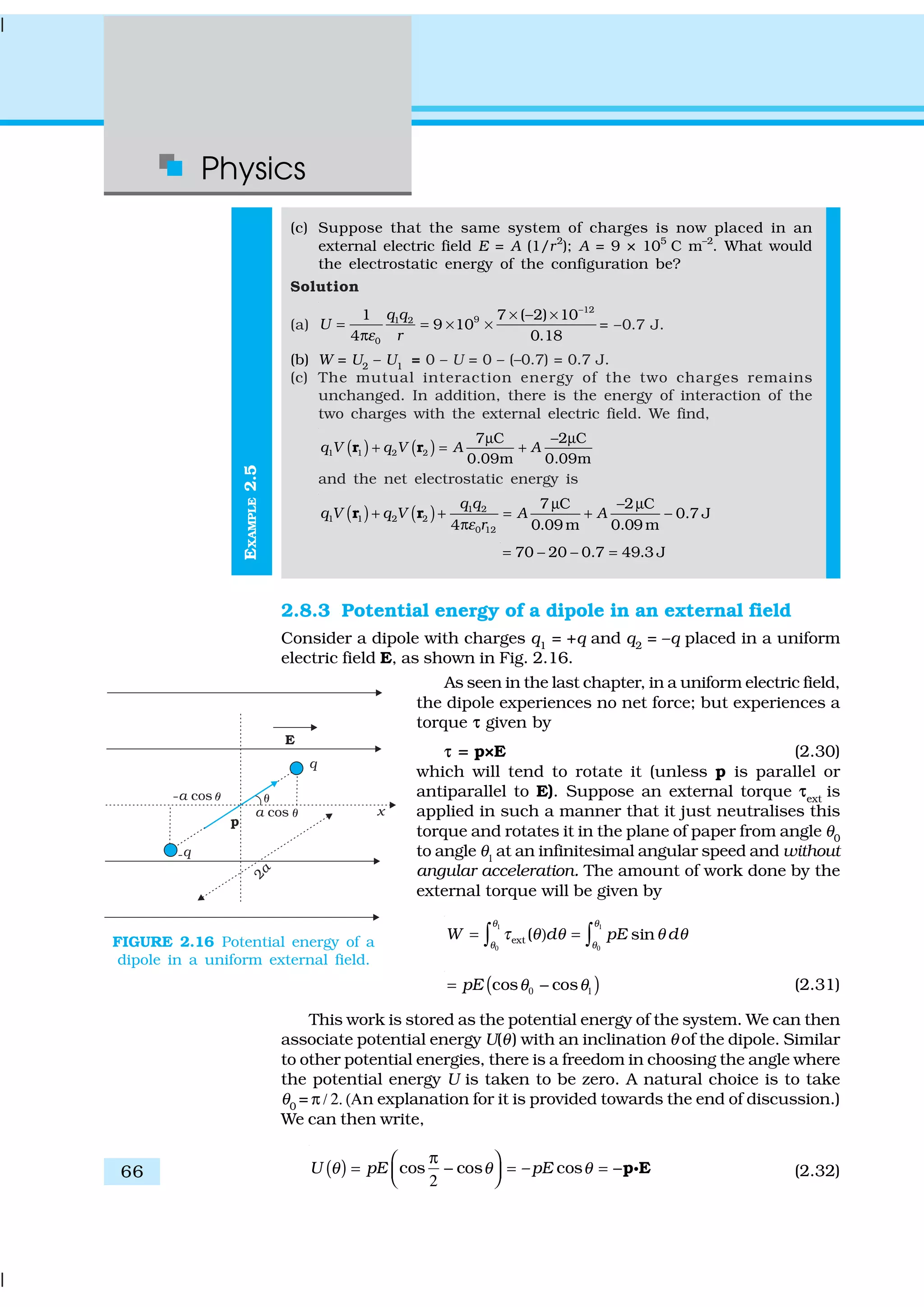
As we learnt in the last chapter, an electric dipole consists of two charges
q and –q separated by a (small) distance 2a. Its total charge is zero. It is
characterised by a dipole moment vector p whose magnitude is q × 2a
and which points in the direction from –q to q (Fig. 2.5). We also saw that
the electric field of a dipole at a point with position vector r depends not
just on the magnitude r, but also on the angle between r and p. Further,
FIGURE 2.4 Variation of potential V with r [in units of
(Q/4πε0
) m-1
] (blue curve) and field with r [in units
of (Q/4πε0
) m-2
] (black curve) for a point charge Q.

60. Physics
56
the field falls off, at large distance, not as
1/r 2
(typical of field due to a single charge)
but as 1/r3
.We, now, determine the electric
potential due to a dipole and contrast it
with the potential due to a single charge.
As before, we take the origin at the
centre of the dipole. Now we know that the
electric field obeys the superposition
principle. Since potential is related to the
work done by the field, electrostatic
potential also follows the superposition
principle. Thus, the potential due to the
dipole is the sum of potentials due to the
charges q and –q
0 1 2
1
4
q q
V
r rε
 
= − π  
(2.9)
where r1
and r2
are the distances of the
point P from q and –q, respectively.
Now, by geometry,
2 2 2
1 2r r a ar= + − cosθ
2 2 2
2 2r r a ar= + + cosθ (2.10)
We take r much greater than a ( ar >> ) and retain terms only upto
the first order in a/r
2
2 2
1 2
2 cos
1
a a
r r
r r
θ 
= − +  
2 2 cos
1
a
r
r
θ 
≅ −   (2.11)
Similarly,
2 2
2
2 cos
1
a
r r
r
θ 
≅ +   (2.12)
Using the Binomial theorem and retaining terms upto the first order
in a/r ; we obtain,
1/2
1
1 1 2 cos 1
1 1 cos
a a
r r r r r
θ
θ
−
   
≅ − ≅ +       [2.13(a)]
1/2
2
1 1 2 cos 1
1 1 cos
a a
r r r r r
θ
θ
−
   
≅ + ≅ −       [2.13(b)]
Using Eqs. (2.9) and (2.13) and p = 2qa, we get
2 2
0 0
2 cos cos
4 4
q a p
V
r r
θ θ
ε ε
= =
π π (2.14)
Now, p cos θ = ˆp rC
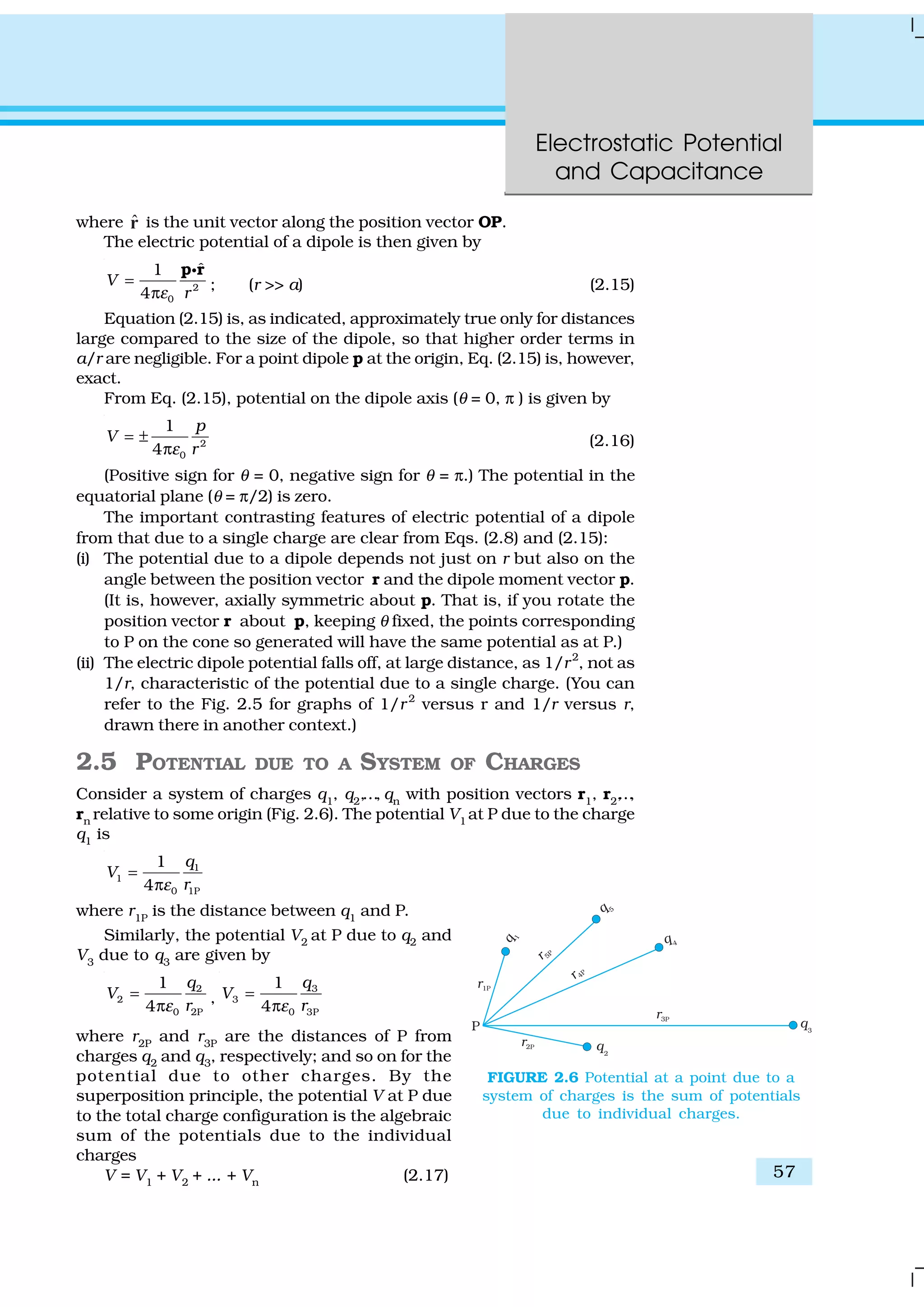
FIGURE 2.5 Quantities involved in the calculation
of potential due to a dipole.

61. Electrostatic Potential
and Capacitance
57
where ˆr is the unit vector along the position vector OP.
The electric potential of a dipole is then given by
2
0
ˆ1
4
V
rε
=
π
p rC
; (r >> a) (2.15)
Equation (2.15) is, as indicated, approximately true only for distances
large compared to the size of the dipole, so that higher order terms in
a/r are negligible. For a point dipole p at the origin, Eq. (2.15) is, however,
exact.
From Eq. (2.15), potential on the dipole axis (θ = 0, π ) is given by
2
0
1
4
p
V
rε
= ±
π
(2.16)
(Positive sign for θ = 0, negative sign for θ = π.) The potential in the
equatorial plane (θ = π/2) is zero.
The important contrasting features of electric potential of a dipole
from that due to a single charge are clear from Eqs. (2.8) and (2.15):
(i) The potential due to a dipole depends not just on r but also on the
angle between the position vector r and the dipole moment vector p.
(It is, however, axially symmetric about p. That is, if you rotate the
position vector r about p, keeping θ fixed, the points corresponding
to P on the cone so generated will have the same potential as at P.)
(ii) The electric dipole potential falls off, at large distance, as 1/r2
, not as
1/r, characteristic of the potential due to a single charge. (You can
refer to the Fig. 2.5 for graphs of 1/r2
versus r and 1/r versus r,
drawn there in another context.)
2.5 POTENTIAL DUE TO A SYSTEM OF CHARGES
Consider a system of charges q1
, q2
,…, qn
with position vectors r1
, r2
,…,
rn relative to some origin (Fig. 2.6). The potential V1 at P due to the charge
q1
is
1
1
0 1P
1
4
q
V
rε
=
π
where r1P
is the distance between q1
and P.
Similarly, the potential V2 at P due to q2 and
V3
due to q3
are given by
2
2
0 2P
1
4
q
V
rε
=
π
,
3
3
0 3P
1
4
q
V
rε
=
π
where r2P
and r3P
are the distances of P from
charges q2 and q3, respectively; and so on for the
potential due to other charges. By the
superposition principle, the potential V at P due
to the total charge configuration is the algebraic
sum of the potentials due to the individual
charges
V = V1 + V2 + ... + Vn (2.17)
FIGURE 2.6 Potential at a point due to a
system of charges is the sum of potentials
due to individual charges.

62. Physics
58
EXAMPLE2.2
1 2
0 1P 2P P
1
......
4
n
n
qq q
r r rε
 
= + + + π  
(2.18)
If we have a continuous charge distribution characterised by a charge
density ρ (r), we divide it, as before, into small volume elements each of
size ∆v and carrying a charge ρ∆v. We then determine the potential due
to each volume element and sum (strictly speaking , integrate) over all
such contributions, and thus determine the potential due to the entire
distribution.
We have seen in Chapter 1 that for a uniformly charged spherical shell,
the electric field outside the shell is as if the entire charge is concentrated
at the centre. Thus, the potential outside the shell is given by
0
1
4
q
V
rε
=
π ( )r R≥ [2.19(a)]
where q is the total charge on the shell and R its radius. The electric field
inside the shell is zero. This implies (Section 2.6) that potential is constant
inside the shell (as no work is done in moving a charge inside the shell),
and, therefore, equals its value at the surface, which is
0
1
4
q
V
Rε
=
π [2.19(b)]
Example 2.2 Two charges 3 × 10–8
C and –2 × 10–8
C are located
15 cm apart. At what point on the line joining the two charges is the
electric potential zero? Take the potential at infinity to be zero.
Solution Let us take the origin O at the location of the positive charge.
The line joining the two charges is taken to be the x-axis; the negative
charge is taken to be on the right side of the origin (Fig. 2.7).
FIGURE 2.7
Let P be the required point on the x-axis where the potential is zero.
If x is the x-coordinate of P, obviously x must be positive. (There is no
possibility of potentials due to the two charges adding up to zero for
x < 0.) If x lies between O and A, we have
–8 –8
–2 –2
0
1 3 10 2 10
0
10 (15 ) 104 ε
× ×
− =
× − ×π
 
 
 x x
where x is in cm. That is,
3 2
0
15x x
− =
−
which gives x = 9 cm.
If x lies on the extended line OA, the required condition is
3 2
0
15x x
− =
−

63. Electrostatic Potential
and Capacitance
59
EXAMPLE2.2
which gives
x = 45 cm
Thus, electric potential is zero at 9 cm and 45 cm away from the
positive charge on the side of the negative charge. Note that the
formula for potential used in the calculation required choosing
potential to be zero at infinity.
Example 2.3 Figures 2.8 (a) and (b) show the field lines of a positive
and negative point charge respectively.
FIGURE 2.8
(a) Give the signs of the potential difference VP
– VQ
; VB
– VA
.
(b) Give the sign of the potential energy difference of a small negative
charge between the points Q and P; A and B.
(c) Give the sign of the work done by the field in moving a small
positive charge from Q to P.
(d) Give the sign of the work done by the external agency in moving
a small negative charge from B to A.
(e) Does the kinetic energy of a small negative charge increase or
decrease in going from B to A?
Solution
(a) As
1
V
r
∝ , VP
> VQ
. Thus, (VP
– VQ
) is positive. Also VB
is less negative
than VA
. Thus, VB
> VA
or (VB
– VA
) is positive.
(b) A small negative charge will be attracted towards positive charge.
The negative charge moves from higher potential energy to lower
potential energy. Therefore the sign of potential energy difference
of a small negative charge between Q and P is positive.
Similarly, (P.E.)A
> (P.E.)B
and hence sign of potential energy
differences is positive.
(c) In moving a small positive charge from Q to P, work has to be
done by an external agency against the electric field. Therefore,
work done by the field is negative.
(d) In moving a small negative charge from B to A work has to be
done by the external agency. It is positive.
(e) Due to force of repulsion on the negative charge, velocity decreases
and hence the kinetic energy decreases in going from B to A.
EXAMPLE2.3
Electricpotential,equipotentialsurfaces:
http://sol.sci.uop.edu/~jfalward/electricpotential/electricpotential.html

64. Physics
60
FIGURE 2.10 Equipotential surfaces for a uniform electric field.
2.6 EQUIPOTENTIAL SURFACES
An equipotential surface is a surface with a constant value of potential
at all points on the surface. For a single charge q, the potential is given
by Eq. (2.8):
1
4 o
q
V
rε
=
π
This shows that V is a constant if r is constant . Thus, equipotential
surfaces of a single point charge are concentric spherical surfaces centred
at the charge.
Now the electric field lines for a single charge q are radial lines starting
from or ending at the charge, depending on whether q is positive or negative.
Clearly, the electric field at every point is normal to the equipotential surface
passing through that point. This is true in general: for any charge
configuration, equipotential surface through a point is normal to the
electric field at that point. The proof of this statement is simple.
If the field were not normal to the equipotential surface, it would
have non-zero component along the surface. To move a unit test charge
against the direction of the component of the field, work would have to
be done. But this is in contradiction to the definition of an equipotential
surface: there is no potential difference between any two points on the
surface and no work is required to move a test charge on the surface.
The electric field must, therefore, be normal to the equipotential surface
at every point. Equipotential surfaces offer an alternative visual picture
in addition to the picture of electric field lines around a charge
configuration.
FIGURE 2.9 For a
single charge q
(a) equipotential
surfaces are
spherical surfaces
centred at the
charge, and
(b) electric field
lines are radial,
starting from the
charge if q > 0.
For a uniform electric field E, say, along the x -axis, the equipotential
surfaces are planes normal to the x -axis, i.e., planes parallel to the y-z
plane (Fig. 2.10). Equipotential surfaces for (a) a dipole and (b) two
identical positive charges are shown in Fig. 2.11.
FIGURE 2.11 Some equipotential surfaces for (a) a dipole,
(b) two identical positive charges.

65. Electrostatic Potential
and Capacitance
61
2.6.1 Relation between field and potential
Consider two closely spaced equipotential surfaces A and B (Fig. 2.12)
with potential values V and V + δV, where δV is the change in V in the
direction of the electric field E. Let P be a point on the
surface B. δl is the perpendicular distance of the
surface A from P. Imagine that a unit positive charge
is moved along this perpendicular from the surface B
to surface A against the electric field. The work done
in this process is |E|δ l.
This work equals the potential difference
VA–VB.
Thus,
|E|δ l = V −(V +δV)= –δV
i.e., |E|=
V
l
δ
δ
− (2.20)
Since δV is negative, δV = – |δV|. we can rewrite
Eq (2.20) as
VV
l l
δδ
δ δ
= − = +E (2.21)
We thus arrive at two important conclusions concerning the relation
between electric field and potential:
(i) Electric field is in the direction in which the potential decreases
steepest.
(ii) Its magnitude is given by the change in the magnitude of potential
per unit displacement normal to the equipotential surface at the point.
2.7 POTENTIAL ENERGY OF A SYSTEM OF CHARGES
Consider first the simple case of two charges q1
and q2
with position vector
r1 and r2 relative to some origin. Let us calculate the work done
(externally) in building up this configuration. This means that we consider
the charges q1
and q2
initially at infinity and determine the work done by
an external agency to bring the charges to the given locations. Suppose,
first the charge q1
is brought from infinity to the point r1
. There is no
external field against which work needs to be done, so work done in
bringing q1 from infinity to r1 is zero. This charge produces a potential in
space given by
1
1
0 1P
1
4
q
V
rε
=
π
where r1P
is the distance of a point P in space from the location of q1
.
From the definition of potential, work done in bringing charge q2 from
infinity to the point r2
is q2
times the potential at r2
due to q1
:
work done on q2
=
1 2
0 12
1
4
q q
rεπ
FIGURE 2.12 From the
potential to the field.

66. Physics
62
where r12
is the distance between points 1 and 2.
Since electrostatic force is conservative, this work gets
stored in the form of potential energy of the system. Thus,
the potential energy of a system of two charges q1
and q2
is
1 2
0 12
1
4
q q
U
rε
=
π
(2.22)
Obviously, if q2
was brought first to its present location and
q1
brought later, the potential energy U would be the same.
More generally, the potential energy expression,
Eq. (2.22), is unaltered whatever way the charges are brought to the specified
locations, because of path-independence of work for electrostatic force.
Equation (2.22) is true for any sign of q1and q2. If q1q2 > 0, potential
energy is positive. This is as expected, since for like charges (q1
q2
> 0),
electrostatic force is repulsive and a positive amount of work is needed to
be done against this force to bring the charges from infinity to a finite
distance apart. For unlike charges (q1
q2
< 0), the electrostatic force is
attractive. In that case, a positive amount of work is needed against this
force to take the charges from the given location to infinity. In other words,
a negative amount of work is needed for the reverse path (from infinity to
the present locations), so the potential energy is negative.
Equation (2.22) is easily generalised for a system of any number of
point charges. Let us calculate the potential energy of a system of three
charges q1
, q2
and q3
located at r1
, r2
, r3
, respectively. To bring q1
first
from infinity to r1, no work is required. Next we bring q2 from infinity to
r2
. As before, work done in this step is
1 2
2 1 2
0 12
1
( )
4
q q
q V
rε
=
π
r (2.23)
The charges q1 and q2 produce a potential, which at any point P is
given by
1 2
1,2
0 1P 2P
1
4
q q
V
r rε
 
= + π  
(2.24)
Work done next in bringing q3
from infinity to the point r3
is q3
times
V1, 2 at r3
1 3 2 3
3 1,2 3
0 13 23
1
( )
4
q q q q
q V
r rε
 
= + π  
r (2.25)
The total work done in assembling the charges
at the given locations is obtained by adding the work
done in different steps [Eq. (2.23) and Eq. (2.25)],
1 3 2 31 2
0 12 13 23
1
4
q q q qq q
U
r r rε
 
= + + π  
(2.26)
Again, because of the conservative nature of the
electrostatic force (or equivalently, the path
independence of work done), the final expression for
U, Eq. (2.26), is independent of the manner in which
the configuration is assembled. The potential energy
FIGURE 2.13 Potential energy of a
system of charges q1
and q2
is
directly proportional to the product
of charges and inversely to the
distance between them.
FIGURE 2.14 Potential energy of a
system of three charges is given by
Eq. (2.26), with the notation given
in the figure.

67. Electrostatic Potential
and Capacitance
63
EXAMPLE2.4
is characteristic of the present state of configuration, and not the way
the state is achieved.
Example 2.4 Four charges are arranged at the corners of a square
ABCD of side d, as shown in Fig. 2.15.(a) Find the work required to
put together this arrangement. (b) A charge q0
is brought to the centre
E of the square, the four charges being held fixed at its corners. How
much extra work is needed to do this?
FIGURE 2.15
Solution
(a) Since the work done depends on the final arrangement of the
charges, and not on how they are put together, we calculate work
needed for one way of putting the charges at A, B, C and D. Suppose,
first the charge +q is brought to A, and then the charges –q, +q, and
–q are brought to B, C and D, respectively. The total work needed can
be calculated in steps:
(i) Work needed to bring charge +q to A when no charge is present
elsewhere: this is zero.
(ii) Work needed to bring –q to B when +q is at A. This is given by
(charge at B) × (electrostatic potential at B due to charge +q at A)
2
0 04 4
q q
q
d dε ε
 
= − × = − π π 
(iii) Work needed to bring charge +q to C when +q is at A and –q is at
B. This is given by (charge at C) × (potential at C due to charges
at A and B)
00
44 2
q q
q
dd εε
 + −
= + + ππ 
2
0
1
1
4 2
q
dε
−  
= −  π
(iv) Work needed to bring –q to D when +q at A,–q at B, and +q at C.
This is given by (charge at D) × (potential at D due to charges at A,
B and C)
0 00
4 44 2
q q q
q
d ddε εε
 + −
= − + + π ππ 
2
0
1
2
4 2
q
dε
−  
= −  π

68. Physics
64
EXAMPLE2.4
Add the work done in steps (i), (ii), (iii) and (iv). The total work
required is
2
0
1 1
(0) (1) 1 2
4 2 2
q
dε
 −    
= + + − + −       π  
( )
2
0
4 2
4
q
dε
−
= −
π
The work done depends only on the arrangement of the charges, and
not how they are assembled. By definition, this is the total
electrostatic energy of the charges.
(Students may try calculating same work/energy by taking charges
in any other order they desire and convince themselves that the energy
will remain the same.)
(b) The extra work necessary to bring a charge q0
to the point E when
the four charges are at A, B, C and D is q0
× (electrostatic potential at
E due to the charges at A, B, C and D). The electrostatic potential at
E is clearly zero since potential due to A and C is cancelled by that
due to B and D. Hence no work is required to bring any charge to
point E.
2.8 POTENTIAL ENERGY IN AN EXTERNAL FIELD
2.8.1 Potential energy of a single charge
In Section 2.7, the source of the electric field was specified – the charges
and their locations - and the potential energy of the system of those charges
was determined. In this section, we ask a related but a distinct question.
What is the potential energy of a charge q in a given field? This question
was, in fact, the starting point that led us to the notion of the electrostatic
potential (Sections 2.1 and 2.2). But here we address this question again
to clarify in what way it is different from the discussion in Section 2.7.
The main difference is that we are now concerned with the potential
energy of a charge (or charges) in an external field. The external field E is
not produced by the given charge(s) whose potential energy we wish to
calculate. E is produced by sources external to the given charge(s).The
external sources may be known, but often they are unknown or
unspecified; what is specified is the electric field E or the electrostatic
potential V due to the external sources. We assume that the charge q
does not significantly affect the sources producing the external field. This
is true if q is very small, or the external sources are held fixed by other
unspecified forces. Even if q is finite, its influence on the external sources
may still be ignored in the situation when very strong sources far away
at infinity produce a finite field E in the region of interest. Note again that
we are interested in determining the potential energy of a given charge q
(and later, a system of charges) in the external field; we are not interested
in the potential energy of the sources producing the external electric field.
The external electric field E and the corresponding external potential
V may vary from point to point. By definition, V at a point P is the work
done in bringing a unit positive charge from infinity to the point P.

69. Electrostatic Potential
and Capacitance
65
EXAMPLE2.5
(We continue to take potential at infinity to be zero.) Thus, work done in
bringing a charge q from infinity to the point P in the external field is qV.
This work is stored in the form of potential energy of q. If the point P has
position vector r relative to some origin, we can write:
Potential energy of q at r in an external field
= qV(r) (2.27)
where V(r) is the external potential at the point r.
Thus, if an electron with charge q = e = 1.6×10–19
C is accelerated by
a potential difference of ∆V = 1 volt, it would gain energy of q∆V = 1.6 ×
10–19
J. This unit of energy is defined as 1 electron volt or 1eV, i.e.,
1 eV=1.6 × 10–19
J. The units based on eV are most commonly used in
atomic, nuclear and particle physics, (1 keV = 103
eV = 1.6 × 10–16
J, 1 MeV
= 106
eV = 1.6 × 10–13
J, 1 GeV = 109
eV = 1.6 × 10–10
J and 1 TeV = 1012
eV
= 1.6 × 10–7
J). [This has already been defined on Page 117, XI Physics
Part I, Table 6.1.]
2.8.2 Potential energy of a system of two charges in an
external field
Next, we ask: what is the potential energy of a system of two charges q1
and q2
located at r1
and r2
, respectively, in an external field? First, we
calculate the work done in bringing the charge q1
from infinity to r1
.
Work done in this step is q1 V(r1), using Eq. (2.27). Next, we consider the
work done in bringing q2
to r2
. In this step, work is done not only against
the external field E but also against the field due to q1
.
Work done on q2 against the external field
= q2
V (r2
)
Work done on q2
against the field due to q1
1 2
124 o
q q
rε
=
π
where r12
is the distance between q1
and q2
. We have made use of Eqs.
(2.27) and (2.22). By the superposition principle for fields, we add up
the work done on q2 against the two fields (E and that due to q1):
Work done in bringing q2
to r2
1 2
2 2
12
( )
4 o
q q
q V
rε
= +
π
r (2.28)
Thus,
Potential energy of the system
= the total work done in assembling the configuration
1 2
1 1 2 2
0 12
( ) ( )
4
q q
q V q V
rε
= + +
π
r r (2.29)
Example 2.5
(a) Determine the electrostatic potential energy of a system consisting
of two charges 7 µC and –2 µC (and with no external field) placed
at (–9 cm, 0, 0) and (9 cm, 0, 0) respectively.
(b) How much work is required to separate the two charges infinitely
away from each other?

70. Physics
66
EXAMPLE2.5
(c) Suppose that the same system of charges is now placed in an
external electric field E = A (1/r2
); A = 9 × 105
C m–2
. What would
the electrostatic energy of the configuration be?
Solution
(a)
12
91 2
0
1 7 ( 2) 10
9 10
4 0.18
q q
U
rε
−
× − ×
= = × ×
π
= –0.7 J.
(b) W = U2
– U1
= 0 – U = 0 – (–0.7) = 0.7 J.
(c) The mutual interaction energy of the two charges remains
unchanged. In addition, there is the energy of interaction of the
two charges with the external electric field. We find,
( ) ( )1 1 2 2
7 C 2 C
0.09m 0.09m
q V q V A A
µ − µ
+ = +r r
and the net electrostatic energy is
( ) ( ) 1 2
1 1 2 2
0 12
7 C 2 C
0.7 J
4 0.09 m 0.09 m
q q
q V q V A A
rε
µ − µ
+ + = + −
π
r r
70 20 0.7 49.3 J= − − =
2.8.3 Potential energy of a dipole in an external field
Consider a dipole with charges q1
= +q and q2
= –q placed in a uniform
electric field E, as shown in Fig. 2.16.
As seen in the last chapter, in a uniform electric field,
the dipole experiences no net force; but experiences a
torque ττ given by
=τ ==τ = p×E (2.30)
which will tend to rotate it (unless p is parallel or
antiparallel to E). Suppose an external torque ττext
is
applied in such a manner that it just neutralises this
torque and rotates it in the plane of paper from angle θ0
to angle θ1
at an infinitesimal angular speed and without
angular acceleration. The amount of work done by the
external torque will be given by
ext ( sinW d pE d
θ θ
θ θ
τ θ θ θ θ
1 1
0 0
= ) =∫ ∫
( )cos cospE θ θ0 1= − (2.31)
This work is stored as the potential energy of the system. We can then
associate potential energy U(θ) with an inclination θ of the dipole. Similar
to other potential energies, there is a freedom in choosing the angle where
the potential energy U is taken to be zero. A natural choice is to take
θ0
= π / 2. (Αn explanation for it is provided towards the end of discussion.)
We can then write,
( ) cos cos – cosU pE pEθ θ θ
π 
= − = = −  2
p EC (2.32)
FIGURE 2.16 Potential energy of a
dipole in a uniform external field.

71. Electrostatic Potential
and Capacitance
67
EXAMPLE2.6
This expression can alternately be understood also from Eq. (2.29).
We apply Eq. (2.29) to the present system of two charges +q and –q. The
potential energy expression then reads
( ) ( ) ( )
2
1 2[ ]
4 2
q
U q V V
a
θ
ε0
= − −′
π ×
r r (2.33)
Here, r1
and r2
denote the position vectors of +q and –q. Now, the
potential difference between positions r1 and r2 equals the work done
in bringing a unit positive charge against field from r2
to r1
. The
displacement parallel to the force is 2a cosθ. Thus, [V(r1
)–V (r2
)] =
–E × 2a cosθ . We thus obtain,
( )
2 2
cos
4 2 4 2
q q
U pE
a a
θ θ
ε ε0 0
= − − = − −′
π × π ×
p EC (2.34)
We note that U′(θ) differs from U(θ ) by a quantity which is just a constant
for a given dipole. Since a constant is insignificant for potential energy, we
can drop the second term in Eq. (2.34) and it then reduces to Eq. (2.32).
We can now understand why we took θ0
=π/2. In this case, the work
done against the external field E in bringing +q and – q are equal and
opposite and cancel out, i.e., q [V (r1) – V (r2)]=0.
Example 2.6 A molecule of a substance has a permanent electric
dipole moment of magnitude 10–29
C m. A mole of this substance is
polarised (at low temperature) by applying a strong electrostatic field
of magnitude 106
V m–1
. The direction of the field is suddenly changed
by an angle of 60º. Estimate the heat released by the substance in
aligning its dipoles along the new direction of the field. For simplicity,
assume 100% polarisation of the sample.
Solution Here, dipole moment of each molecules = 10–29
C m
As 1 mole of the substance contains 6 × 1023
molecules,
total dipole moment of all the molecules, p = 6 × 1023
× 10–29
C m
= 6 × 10–6
C m
Initial potential energy, Ui
= –pE cos θ = –6×10–6
×106
cos 0° = –6 J
Final potential energy (when θ = 60°), Uf
= –6 × 10–6
× 106
cos 60° = –3 J
Change in potential energy = –3 J – (–6J) = 3 J
So, there is loss in potential energy. This must be the energy released
by the substance in the form of heat in aligning its dipoles.
2.9 ELECTROSTATICS OF CONDUCTORS
Conductors and insulators were described briefly in Chapter 1.
Conductors contain mobile charge carriers. In metallic conductors, these
charge carriers are electrons. In a metal, the outer (valence) electrons
part away from their atoms and are free to move. These electrons are free
within the metal but not free to leave the metal. The free electrons form a
kind of ‘gas’; they collide with each other and with the ions, and move
randomly in different directions. In an external electric field, they drift
against the direction of the field. The positive ions made up of the nuclei
and the bound electrons remain held in their fixed positions. In electrolytic
conductors, the charge carriers are both positive and negative ions; but

72. Physics
68
the situation in this case is more involved – the movement of the charge
carriers is affected both by the external electric field as also by the
so-called chemical forces (see Chapter 3). We shall restrict our discussion
to metallic solid conductors. Let us note important results regarding
electrostatics of conductors.
1. Inside a conductor, electrostatic field is zero
Consider a conductor, neutral or charged. There may also be an external
electrostatic field. In the static situation, when there is no current inside
or on the surface of the conductor, the electric field is zero everywhere
inside the conductor. This fact can be taken as the defining property of a
conductor. A conductor has free electrons. As long as electric field is not
zero, the free charge carriers would experience force and drift. In the
static situation, the free charges have so distributed themselves that the
electric field is zero everywhere inside. Electrostatic field is zero inside a
conductor.
2. At the surface of a charged conductor, electrostatic field
must be normal to the surface at every point
If E were not normal to the surface, it would have some non-zero
component along the surface. Free charges on the surface of the conductor
would then experience force and move. In the static situation, therefore,
E should have no tangential component. Thus electrostatic field at the
surface of a charged conductor must be normal to the surface at every
point. (For a conductor without any surface charge density, field is zero
even at the surface.) See result 5.
3. The interior of a conductor can have no excess charge in
the static situation
A neutral conductor has equal amounts of positive and negative charges
in every small volume or surface element. When the conductor is charged,
the excess charge can reside only on the surface in the static situation.
This follows from the Gauss’s law. Consider any arbitrary volume element
v inside a conductor. On the closed surface S bounding the volume
element v, electrostatic field is zero. Thus the total electric flux through S
is zero. Hence, by Gauss’s law, there is no net charge enclosed by S. But
the surface S can be made as small as you like, i.e., the volume v can be
made vanishingly small. This means there is no net charge at any point
inside the conductor, and any excess charge must reside at the surface.
4. Electrostatic potential is constant throughout the volume
of the conductor and has the same value (as inside) on
its surface
This follows from results 1 and 2 above. Since E = 0 inside the conductor
and has no tangential component on the surface, no work is done in
moving a small test charge within the conductor and on its surface. That
is, there is no potential difference between any two points inside or on
the surface of the conductor. Hence, the result. If the conductor is charged,

73. Electrostatic Potential
and Capacitance
69
electric field normal to the surface exists; this means potential will be
different for the surface and a point just outside the surface.
In a system of conductors of arbitrary size, shape and
charge configuration, each conductor is characterised by a constant
value of potential, but this constant may differ from one conductor to
the other.
5. Electric field at the surface of a charged conductor
0
ˆ
σ
ε
=E n (2.35)
where σ is the surface charge density and ˆn is a unit vector normal
to the surface in the outward direction.
To derive the result, choose a pill box (a short cylinder) as the Gaussian
surface about any point P on the surface, as shown in Fig. 2.17. The pill
box is partly inside and partly outside the surface of the conductor. It
has a small area of cross section δ S and negligible height.
Just inside the surface, the electrostatic field is zero; just outside, the
field is normal to the surface with magnitude E. Thus,
the contribution to the total flux through the pill box
comes only from the outside (circular) cross-section
of the pill box. This equals ± EδS (positive for σ > 0,
negative for σ < 0), since over the small area δS, E
may be considered constant and E and δS are parallel
or antiparallel. The charge enclosed by the pill box
is σδS.
By Gauss’s law
EδS =
0
Sσ δ
ε
E =
0
σ
ε
(2.36)
Including the fact that electric field is normal to the
surface, we get the vector relation, Eq. (2.35), which
is true for both signs of σ. For σ > 0, electric field is
normal to the surface outward; for σ < 0, electric field
is normal to the surface inward.
6. Electrostatic shielding
Consider a conductor with a cavity, with no charges inside the cavity. A
remarkable result is that the electric field inside the cavity is zero, whatever
be the size and shape of the cavity and whatever be the charge on the
conductor and the external fields in which it might be placed. We have
proved a simple case of this result already: the electric field inside a charged
spherical shell is zero. The proof of the result for the shell makes use of
the spherical symmetry of the shell (see Chapter 1). But the vanishing of
electric field in the (charge-free) cavity of a conductor is, as mentioned
above, a very general result. A related result is that even if the conductor
FIGURE 2.17 The Gaussian surface
(a pill box) chosen to derive Eq. (2.35)
for electric field at the surface of a
charged conductor.

74. Physics
70
EXAMPLE2.7
FIGURE 2.18 The electric field inside a
cavity of any conductor is zero. All
charges reside only on the outer surface
of a conductor with cavity. (There are no
charges placed in the cavity.)
is charged or charges are induced on a neutral
conductor by an external field, all charges reside
only on the outer surface of a conductor with cavity.
The proofs of the results noted in Fig. 2.18 are
omitted here, but we note their important
implication. Whatever be the charge and field
configuration outside, any cavity in a conductor
remains shielded from outside electric influence: the
field inside the cavity is always zero. This is known
as electrostatic shielding. The effect can be made
use of in protecting sensitive instruments from
outside electrical influence. Figure 2.19 gives a
summary of the important electrostatic properties
of a conductor.
Example 2.7
(a) A comb run through one’s dry hair attracts small bits of paper.
Why?
What happens if the hair is wet or if it is a rainy day? (Remember,
a paper does not conduct electricity.)
(b) Ordinary rubber is an insulator. But special rubber tyres of
aircraft are made slightly conducting. Why is this necessary?
(c) Vehicles carrying inflammable materials usually have metallic
ropes touching the ground during motion. Why?
(d) A bird perches on a bare high power line, and nothing happens
to the bird. A man standing on the ground touches the same line
and gets a fatal shock. Why?
Solution
(a) This is because the comb gets charged by friction. The molecules
in the paper gets polarised by the charged comb, resulting in a
net force of attraction. If the hair is wet, or if it is rainy day, friction
between hair and the comb reduces. The comb does not get
charged and thus it will not attract small bits of paper.
FIGURE 2.19 Some important electrostatic properties of a conductor.

75. Electrostatic Potential
and Capacitance
71
EXAMPLE2.7
(b) To enable them to conduct charge (produced by friction) to the
ground; as too much of static electricity accumulated may result
in spark and result in fire.
(c) Reason similar to (b).
(d) Current passes only when there is difference in potential.
2.10 DIELECTRICS AND POLARISATION
Dielectrics are non-conducting substances. In contrast to conductors,
they have no (or negligible number of ) charge carriers. Recall from Section
2.9 what happens when a conductor is placed in an
external electric field. The free charge carriers move
and charge distribution in the conductor adjusts
itself in such a way that the electric field due to
induced charges opposes the external field within
the conductor. This happens until, in the static
situation, the two fields cancel each other and the
net electrostatic field in the conductor is zero. In a
dielectric, this free movement of charges is not
possible. It turns out that the external field induces
dipole moment by stretching or re-orienting
molecules of the dielectric. The collective effect of all
the molecular dipole moments is net charges on the
surface of the dielectric which produce a field that
opposes the external field. Unlike in a conductor,
however, the opposing field so induced does not
exactly cancel the external field. It only reduces it.
The extent of the effect depends on the
nature of the dielectric. To understand the
effect, we need to look at the charge
distribution of a dielectric at the
molecular level.
The molecules of a substance may be
polar or non-polar. In a non-polar
molecule, the centres of positive and
negative charges coincide. The molecule
then has no permanent (or intrinsic) dipole
moment. Examples of non-polar molecules
are oxygen (O2
) and hydrogen (H2
)
molecules which, because of their
symmetry, have no dipole moment. On the
other hand, a polar molecule is one in which
the centres of positive and negative charges
are separated (even when there is no
external field). Such molecules have a
permanent dipole moment. An ionic
molecule such as HCl or a molecule of water
(H2
O) are examples of polar molecules.
FIGURE 2.20 Difference in behaviour
of a conductor and a dielectric
in an external electric field.
FIGURE 2.21 Some examples of polar
and non-polar molecules.

76. Physics
72
In an external electric field, the
positive and negative charges of a non-
polar molecule are displaced in opposite
directions. The displacement stops when
the external force on the constituent
charges of the molecule is balanced by
the restoring force (due to internal fields
in the molecule). The non-polar molecule
thus develops an induced dipole moment.
The dielectric is said to be polarised by
the external field. We consider only the
simple situation when the induced dipole
moment is in the direction of the field and
is proportional to the field strength.
(Substances for which this assumption
is true are called linear isotropic
dielectrics.) The induced dipole moments
of different molecules add up giving a net
dipole moment of the dielectric in the
presence of the external field.
A dielectric with polar molecules also
develops a net dipole moment in an
external field, but for a different reason.
In the absence of any external field, the
different permanent dipoles are oriented
randomly due to thermal agitation; so
the total dipole moment is zero. When
an external field is applied, the individual dipole moments tend to align
with the field. When summed over all the molecules, there is then a net
dipole moment in the direction of the external field, i.e., the dielectric is
polarised. The extent of polarisation depends on the relative strength of
two mutually opposite factors: the dipole potential energy in the external
field tending to align the dipoles with the field and thermal energy tending
to disrupt the alignment. There may be, in addition, the ‘induced dipole
moment’ effect as for non-polar molecules, but generally the alignment
effect is more important for polar molecules.
Thus in either case, whether polar or non-polar, a dielectric develops
a net dipole moment in the presence of an external field. The dipole
moment per unit volume is called polarisation and is denoted by P. For
linear isotropic dielectrics,
eχ=P E (2.37)
where χe
is a constant characteristic of the dielectric and is known as the
electric susceptibility of the dielectric medium.
It is possible to relate χe
to the molecular properties of the substance,
but we shall not pursue that here.
The question is: how does the polarised dielectric modify the original
external field inside it? Let us consider, for simplicity, a rectangular
dielectric slab placed in a uniform external field E0 parallel to two of its
faces. The field causes a uniform polarisation P of the dielectric. Thus
FIGURE 2.22 A dielectric develops a net dipole
moment in an external electric field. (a) Non-polar
molecules, (b) Polar molecules.

77. Electrostatic Potential
and Capacitance
73
every volume element ∆v of the slab has a dipole moment
P ∆v in the direction of the field. The volume element ∆v is
macroscopically small but contains a very large number of
molecular dipoles. Anywhere inside the dielectric, the
volume element ∆v has no net charge (though it has net
dipole moment). This is, because, the positive charge of one
dipole sits close to the negative charge of the adjacent dipole.
However, at the surfaces of the dielectric normal to the
electric field, there is evidently a net charge density. As seen
in Fig 2.23, the positive ends of the dipoles remain
unneutralised at the right surface and the negative ends at
the left surface. The unbalanced charges are the induced
charges due to the external field.
Thus the polarised dielectric is equivalent to two charged
surfaces with induced surface charge densities, say σp
and –σp
. Clearly, the field produced by these surface charges
opposes the external field. The total field in the dielectric
is, thereby, reduced from the case when no dielectric is
present. We should note that the surface charge density
±σp
arises from bound (not free charges) in the dielectric.
2.11 CAPACITORS AND CAPACITANCE
A capacitor is a system of two conductors separated by an insulator
(Fig. 2.24). The conductors have charges, say Q1
and Q2
, and potentials
V1 and V2. Usually, in practice, the two conductors have charges Q
and – Q, with potential difference V = V1
– V2
between them. We shall
consider only this kind of charge configuration of the capacitor. (Even a
single conductor can be used as a capacitor by assuming the other at
infinity.) The conductors may be so charged by connecting them to the
two terminals of a battery. Q is called the charge of the capacitor, though
this, in fact, is the charge on one of the conductors – the total charge of
the capacitor is zero.
The electric field in the region between the
conductors is proportional to the charge Q. That
is, if the charge on the capacitor is, say doubled,
the electric field will also be doubled at every point.
(This follows from the direct proportionality
between field and charge implied by Coulomb’s
law and the superposition principle.) Now,
potential difference V is the work done per unit
positive charge in taking a small test charge from
the conductor 2 to 1 against the field.
Consequently, V is also proportional to Q, and
the ratio Q/V is a constant:
Q
C
V
= (2.38)
The constant C is called the capacitance of the capacitor. C is independent
of Q or V, as stated above. The capacitance C depends only on the
FIGURE 2.23 A uniformly
polarised dielectric amounts
to induced surface charge
density, but no volume
charge density.
FIGURE 2.24 A system of two conductors
separated by an insulator forms a capacitor.

78. Physics
74
geometrical configuration (shape, size, separation) of the system of two
conductors. [As we shall see later, it also depends on the nature of the
insulator (dielectric) separating the two conductors.] The SI unit of
capacitance is 1 farad (=1 coulomb volt-1
) or 1 F = 1 C V–1
. A capacitor
with fixed capacitance is symbolically shown as ---||---, while the one with
variable capacitance is shown as .
Equation (2.38) shows that for large C, V is small for a given Q. This
means a capacitor with large capacitance can hold large amount of charge
Q at a relatively small V. This is of practical importance. High potential
difference implies strong electric field around the conductors. A strong
electric field can ionise the surrounding air and accelerate the charges so
produced to the oppositely charged plates, thereby neutralising the charge
on the capacitor plates, at least partly. In other words, the charge of the
capacitor leaks away due to the reduction in insulating power of the
intervening medium.
The maximum electric field that a dielectric medium can withstand
without break-down (of its insulating property) is called its dielectric
strength; for air it is about 3 × 106
Vm–1
. For a separation between
conductors of the order of 1 cm or so, this field corresponds to a potential
difference of 3 × 104
V between the conductors. Thus, for a capacitor to
store a large amount of charge without leaking, its capacitance should
be high enough so that the potential difference and hence the electric
field do not exceed the break-down limits. Put differently, there is a limit
to the amount of charge that can be stored on a given capacitor without
significant leaking. In practice, a farad is a very big unit; the most common
units are its sub-multiples 1 µF = 10–6
F, 1 nF = 10–9
F, 1 pF = 10–12
F,
etc. Besides its use in storing charge, a capacitor is a key element of most
ac circuits with important functions, as described in Chapter 7.
2.12 THE PARALLEL PLATE CAPACITOR
A parallel plate capacitor consists of two large plane parallel conducting
plates separated by a small distance (Fig. 2.25). We first take the
intervening medium between the plates to be
vacuum. The effect of a dielectric medium between
the plates is discussed in the next section. Let A be
the area of each plate and d the separation between
them. The two plates have charges Q and –Q. Since
d is much smaller than the linear dimension of the
plates (d2
<< A), we can use the result on electric
field by an infinite plane sheet of uniform surface
charge density (Section 1.15). Plate 1 has surface
charge density σ = Q/A and plate 2 has a surface
charge density –σ. Using Eq. (1.33), the electric field
in different regions is:
Outer region I (region above the plate 1),
0 0
0
2 2
E
σ σ
ε ε
= − = (2.39)
FIGURE 2.25 The parallel plate capacitor.

79. Electrostatic Potential
and Capacitance
75
Outer region II (region below the plate 2),
0 0
0
2 2
E
σ σ
ε ε
= − = (2.40)
In the inner region between the plates 1 and 2, the electric fields due
to the two charged plates add up, giving
0 0 0 02 2
Q
E
A
σ σ σ
ε ε ε ε
= + = = (2.41)
The direction of electric field is from the positive to the negative plate.
Thus, the electric field is localised between the two plates and is
uniform throughout. For plates with finite area, this will not be true near
the outer boundaries of the plates. The field lines bend outward at the
edges – an effect called ‘fringing of the field’. By the same token, σ will not
be strictly uniform on the entire plate. [E and σ are related by Eq. (2.35).]
However, for d2
<< A, these effects can be ignored in the regions sufficiently
far from the edges, and the field there is given by Eq. (2.41). Now for
uniform electric field, potential difference is simply the electric field times
the distance between the plates, that is,
0
1 Qd
V E d
Aε
= = (2.42)
The capacitance C of the parallel plate capacitor is then
Q
C
V
= =
0 A
d
ε
= (2.43)
which, as expected, depends only on the geometry of the system. For
typical values like A = 1 m2
, d = 1 mm, we get
12 2 –1 –2 2
9
3
8.85 10 C N m 1m
8.85 10 F
10 m
C
−
−
−
× ×
= = × (2.44)
(You can check that if 1F= 1C V–1
= 1C (NC–1
m)–1
= 1 C2
N–1
m–1
.)
This shows that 1F is too big a unit in practice, as remarked earlier.
Another way of seeing the ‘bigness’ of 1F is to calculate the area of the
plates needed to have C = 1F for a separation of, say 1 cm:
0
Cd
A
ε
= =
2
9 2
12 2 –1 –2
1F 10 m
10 m
8.85 10 C N m
−
−
×
=
×
(2.45)
which is a plate about 30 km in length and breadth!
2.13 EFFECT OF DIELECTRIC ON CAPACITANCE
With the understanding of the behavior of dielectrics in an external field
developed in Section 2.10, let us see how the capacitance of a parallel
plate capacitor is modified when a dielectric is present. As before, we
have two large plates, each of area A, separated by a distance d. The
charge on the plates is ±Q, corresponding to the charge density ±σ (with
σ = Q/A). When there is vacuum between the plates,
0
0
E
σ
ε
=
Factorsaffectingcapacitance,capacitorsinaction
InteractiveJavatutorial
http://micro.magnet.fsa.edu/electromag/java/capacitance/

80. Physics
76
and the potential difference V0
is
V0
= E0
d
The capacitance C0 in this case is
0 0
0
Q A
C
V d
ε= = (2.46)
Consider next a dielectric inserted between the plates fully occupying
the intervening region. The dielectric is polarised by the field and, as
explained in Section 2.10, the effect is equivalent to two charged sheets
(at the surfaces of the dielectric normal to the field) with surface charge
densities σp
and –σp
. The electric field in the dielectric then corresponds
to the case when the net surface charge density on the plates is ±(σ – σp
).
That is,
0
P
E
σ σ
ε
−
= (2.47)
so that the potential difference across the plates is
0
P
V E d d
σ σ
ε
−
= = (2.48)
For linear dielectrics, we expect σp
to be proportional to E0
, i.e., to σ.
Thus, (σ – σp) is proportional to σ and we can write
P
K
σ
σ σ− = (2.49)
where K is a constant characteristic of the dielectric. Clearly, K > 1. We
then have
0 0
d Qd
V
K A K
σ
ε ε
= = (2.50)
The capacitance C, with dielectric between the plates, is then
0KAQ
C
V d
ε
= = (2.51)
The product ε0
K is called the permittivity of the medium and is
denoted by ε
ε = ε0 K (2.52)
For vacuum K = 1 and ε = ε0
; ε0
is called the permittivity of the vacuum.
The dimensionless ratio
0
K
ε
ε
= (2.53)
is called the dielectric constant of the substance. As remarked before,
from Eq. (2.49), it is clear that K is greater than 1. From Eqs. (2.46) and
(2. 51)
0
C
K
C
= (2.54)
Thus, the dielectric constant of a substance is the factor (>1) by which
the capacitance increases from its vacuum value, when the dielectric is
inserted fully between the plates of a capacitor. Though we arrived at

81. Electrostatic Potential
and Capacitance
77
EXAMPLE2.8
Eq. (2.54) for the case of a parallel plate capacitor, it holds good for any
type of capacitor and can, in fact, be viewed in general as a definition of
the dielectric constant of a substance.
ELECTRIC DISPLACEMENT
We have introduced the notion of dielectric constant and arrived at Eq. (2.54), without
giving the explicit relation between the induced charge density σp and the polarisation P.
We take without proof the result that
P
ˆσ = P nC
where ˆn is a unit vector along the outward normal to the surface. Above equation is
general, true for any shape of the dielectric. For the slab in Fig. 2.23, P is along ˆn at the
right surface and opposite to ˆn at the left surface. Thus at the right surface, induced
charge density is positive and at the left surface, it is negative, as guessed already in our
qualitative discussion before. Putting the equation for electric field in vector form
0
ˆ
ˆ
σ
ε
−
=
P n
E n
C
C
or (ε0 E + P) ˆnC =σ
The quantity ε0
E + P is called the electric displacement and is denoted by D. It is a
vector quantity. Thus,
D = ε0 E + P, D ˆnC = σ,
The significance of D is this : in vacuum, E is related to the free charge density σ.
When a dielectric medium is present, the corresponding role is taken up by D. For a
dielectric medium, it is D not E that is directly related to free charge density σ, as seen in
above equation. Since P is in the same direction as E, all the three vectors P, E and D are
parallel.
The ratio of the magnitudes of D and E is
0
0
P
D
K
E
σε
ε
σ σ
= =
−
Thus,
D = ε0
K E
and P = D –ε0E = ε0 (K –1)E
This gives for the electric susceptibility χe
defined in Eq. (2.37)
χe =ε0 (K–1)
Example 2.8 A slab of material of dielectric constant K has the same
area as the plates of a parallel-plate capacitor but has a thickness
(3/4)d, where d is the separation of the plates. How is the capacitance
changed when the slab is inserted between the plates?
Solution Let E0
= V0
/d be the electric field between the plates when
there is no dielectric and the potential difference is V0
. If the dielectric
is now inserted, the electric field in the dielectric will be E = E0
/K.
The potential difference will then be

82. Physics
78
EXAMPLE2.8
0
0
1 3
( ) ( )
4 4
E
V E d d
K
= +
0 0
1 3 3
( )
4 4 4
K
E d V
K K
+
= + =
The potential difference decreases by the factor (K + 3)/4K while the
free charge Q0
on the plates remains unchanged. The capacitance
thus increases
0 0
0
0
4 4
3 3
Q QK K
C C
V K V K
= = =
+ +
2.14 COMBINATION OF CAPACITORS
We can combine several capacitors of capacitance C1, C2,…,Cn to obtain
a system with some effective capacitance C. The effective capacitance
depends on the way the individual capacitors are combined. Two simple
possibilities are discussed below.
2.14.1 Capacitors in series
Figure 2.26 shows capacitors C1 and C2 combined in series.
The left plate of C1
and the right plate of C2
are connected to two
terminals of a battery and have charges Q and –Q ,
respectively. It then follows that the right plate ofC1
has charge –Q and the left plate of C2
has charge Q.
If this was not so, the net charge on each capacitor
would not be zero. This would result in an electric
field in the conductor connecting C1
and C2
. Charge
would flow until the net charge on both C1
and C2
is zero and there is no electric field in the conductor
connecting C1
and C2
. Thus, in the series
combination, charges on the two plates (±Q) are the
same on each capacitor. The total potential drop V
across the combination is the sum of the potential
drops V1
and V2
across C1
and C2
, respectively.
V = V1
+ V2
=
1 2
Q Q
C C
+ (2.55)
i.e.,
1 2
1 1V
Q C C
= + , (2.56)
Now we can regard the combination as an
effective capacitor with charge Q and potential
difference V. The effective capacitance of the
combination is
Q
C
V
= (2.57)
We compare Eq. (2.57) with Eq. (2.56), and
obtain
1 2
1 1 1
C C C
= + (2.58)
FIGURE 2.26 Combination of two
capacitors in series.
FIGURE 2.27 Combination of n
capacitors in series.

83. Electrostatic Potential
and Capacitance
79
EXAMPLE2.9
The proof clearly goes through for any number of
capacitors arranged in a similar way. Equation (2.55),
for n capacitors arranged in series, generalises to
1 2 n
1 2 n
... ...
Q Q Q
V V V V
C C C
= + + + = + + + (2.59)
Following the same steps as for the case of two
capacitors, we get the general formula for effective
capacitance of a series combination of n capacitors:
1 2 3 n
1 1 1 1 1
...
C C C C C
= + + + + (2.60)
2.14.2 Capacitors in parallel
Figure 2.28 (a) shows two capacitors arranged in
parallel. In this case, the same potential difference is
applied across both the capacitors. But the plate charges
(±Q1) on capacitor 1 and the plate charges (±Q2) on the
capacitor 2 are not necessarily the same:
Q1
= C1
V, Q2
= C2
V (2.61)
The equivalent capacitor is one with charge
Q = Q1 + Q2 (2.62)
and potential difference V.
Q = CV = C1
V + C2
V (2.63)
The effective capacitance C is, from Eq. (2.63),
C = C1
+ C2
(2.64)
The general formula for effective capacitance C for
parallel combination of n capacitors [Fig. 2.28 (b)]
follows similarly,
Q = Q1
+ Q2
+ ... + Qn
(2.65)
i.e., CV = C1
V + C2
V + ... Cn
V (2.66)
which gives
C = C1
+ C2
+ ... Cn
(2.67)
Example 2.9 A network of four 10 µF capacitors is connected to a 500 V
supply, as shown in Fig. 2.29. Determine (a) the equivalent capacitance
of the network and (b) the charge on each capacitor. (Note, the charge
on a capacitor is the charge on the plate with higher potential, equal
and opposite to the charge on the plate with lower potential.)
FIGURE 2.28 Parallel combination of
(a) two capacitors, (b) n capacitors.
FIGURE 2.29

84. Physics
80
EXAMPLE2.9
Solution
(a) In the given network, C1
, C2
and C3
are connected in series. The
effective capacitance C′ of these three capacitors is given by
1 2 3
1 1 1 1
C C C C
= + +
′
For C1
= C2
= C3
= 10 µF, C′ = (10/3) µF. The network has C′ and C4
connected in parallel. Thus, the equivalent capacitance C of the
network is
C = C′ + C4
=
10
10
3
 
+  
µF =13.3µF
(b) Clearly, from the figure, the charge on each of the capacitors, C1
,
C2
and C3
is the same, say Q. Let the charge on C4
be Q′. Now, since
the potential difference across AB is Q/C1
, across BC is Q/C2
, across
CD is Q/C3
, we have
1 2 3
500 V
Q Q Q
C C C
+ + = .
Also, Q′/C4
= 500 V.
This gives for the given value of the capacitances,
310
500 F 1.7 10 C
3
Q V −
= × µ = × and
3
500 10 F 5.0 10 CQ V −
= × µ = ×′
2.15 ENERGY STORED IN A CAPACITOR
A capacitor, as we have seen above, is a system of two conductors with
charge Q and –Q. To determine the energy stored in this configuration,
consider initially two uncharged conductors 1 and 2. Imagine next a
process of transferring charge from conductor 2 to conductor 1 bit by
bit, so that at the end, conductor 1 gets charge Q. By
charge conservation, conductor 2 has charge –Q at
the end (Fig 2.30 ).
In transferring positive charge from conductor 2
to conductor 1, work will be done externally, since at
any stage conductor 1 is at a higher potential than
conductor 2. To calculate the total work done, we first
calculate the work done in a small step involving
transfer of an infinitesimal (i.e., vanishingly small)
amount of charge. Consider the intermediate situation
when the conductors 1 and 2 have charges Q′ and
–Q′ respectively. At this stage, the potential difference
V′ between conductors 1 to 2 is Q′/C, where C is the
capacitance of the system. Next imagine that a small
charge δ Q′ is transferred from conductor 2 to 1. Work
done in this step (δ W′), resulting in charge Q′ on
conductor 1 increasing to Q′+ δ Q′, is given by
Q
W V Q Q
C
δ δ δ
′
= =′ ′ ′ (2.68)
FIGURE 2.30 (a) Work done in a small
step of building charge on conductor 1
from Q′ to Q′ + δ Q′. (b) Total work done
in charging the capacitor may be
viewed as stored in the energy of
electric field between the plates.

85. Electrostatic Potential
and Capacitance
81
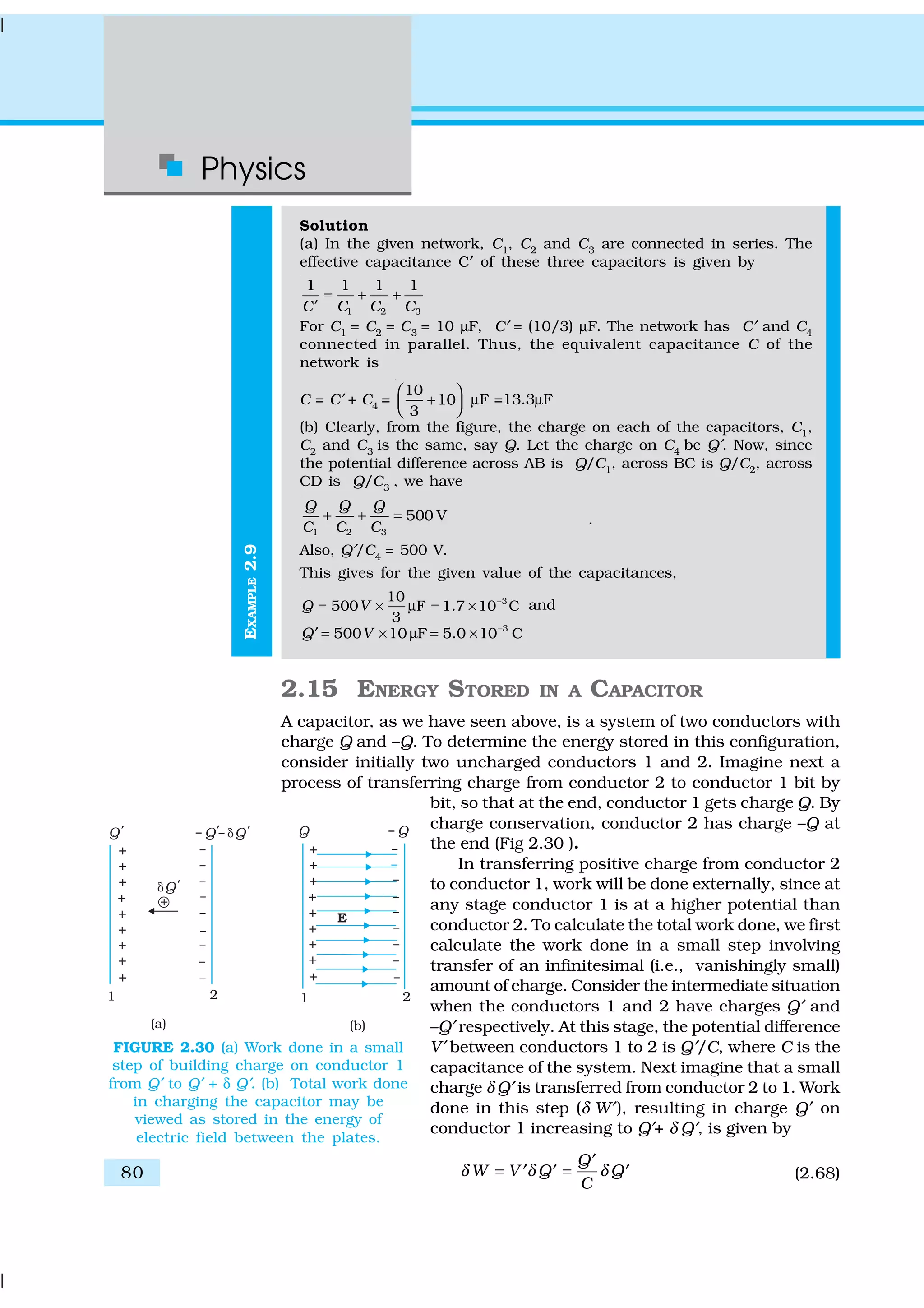
Since δQ′ can be made as small as we like, Eq. (2.68) can be written as
2 21
[( ) ]
2
W Q Q Q
C
δ δ= + −′ ′ ′ (2.69)
Equations (2.68) and (2.69) are identical because the term of second
order in δ Q′, i.e., δ Q′ 2
/2C, is negligible, since δ Q′ is arbitrarily small. The
total work done (W) is the sum of the small work (δ W) over the very large
number of steps involved in building the charge Q′ from zero to Q.
sum over all steps
W Wδ= ∑
=
2 2
sum over all steps
1
[( ) ]
2
Q Q Q
C
δ+ −′ ′ ′∑ (2.70)
=
2 2 21
[{ 0} {(2 ) }
2
Q Q Q
C
δ δ δ− + −′ ′ ′ 2 2
{(3 ) (2 ) } ...Q Qδ δ+ − +′ ′
2 2
{ ( ) }]Q Q Qδ+ − − (2.71)
2
21
[ 0]
2 2
Q
Q
C C
= − = (2.72)
The same result can be obtained directly from Eq. (2.68) by integration
2 2
0 0
1
'
2 2
QQ
Q Q Q
W Q
C C C
δ
′ ′
= = =∫
This is not surprising since integration is nothing but summation of
a large number of small terms.
We can write the final result, Eq. (2.72) in different ways
2
21 1
2 2 2
Q
W CV QV
C
= = = (2.73)
Since electrostatic force is conservative, this work is stored in the form
of potential energy of the system. For the same reason, the final result for
potential energy [Eq. (2.73)] is independent of the manner in which the
charge configuration of the capacitor is built up. When the capacitor
discharges, this stored-up energy is released. It is possible to view the
potential energy of the capacitor as ‘stored’ in the electric field between
the plates. To see this, consider for simplicity, a parallel plate capacitor
[of area A(of each plate) and separation d between the plates].
Energy stored in the capacitor
=
2 2
0
1 ( )
2 2
Q A d
C A
σ
ε
= × (2.74)
The surface charge density σ is related to the electric field E between
the plates,
0
E
σ
ε
= (2.75)
From Eqs. (2.74) and (2.75) , we get
Energy stored in the capacitor
U = ( ) 2
01/2 E A dε × (2.76)

86. Physics
82
EXAMPLE2.10
Note that Ad is the volume of the region between the plates (where
electric field alone exists). If we define energy density as energy stored
per unit volume of space, Eq (2.76) shows that
Energy density of electric field,
u =(1/2)ε0E2
(2.77)
Though we derived Eq. (2.77) for the case of a parallel plate capacitor,
the result on energy density of an electric field is, in fact, very general and
holds true for electric field due to any configuration of charges.
Example 2.10 (a) A 900 pF capacitor is charged by 100 V battery
[Fig. 2.31(a)]. How much electrostatic energy is stored by the capacitor?
(b) The capacitor is disconnected from the battery and connected to
another 900 pF capacitor [Fig. 2.31(b)]. What is the electrostatic energy
stored by the system?
FIGURE 2.31
Solution
(a) The charge on the capacitor is
Q = CV = 900 × 10–12
F × 100 V = 9 × 10–8
C
The energy stored by the capacitor is
= (1/2) CV2
= (1/2) QV
= (1/2) × 9 × 10–8
C × 100 V = 4.5 × 10–6
J
(b) In the steady situation, the two capacitors have their positive
plates at the same potential, and their negative plates at the
same potential. Let the common potential difference be V′. The
charge on each capacitor is then Q′ = CV′. By charge conservation,
Q′ = Q/2. This implies V′ = V/2. The total energy of the system is
61 1
2 ' ' 2.25 10 J
2 4
Q V QV −
= × = = ×
Thus in going from (a) to (b), though no charge is lost; the final
energy is only half the initial energy. Where has the remaining
energy gone?
There is a transient period before the system settles to the
situation (b). During this period, a transient current flows from
the first capacitor to the second. Energy is lost during this time
in the form of heat and electromagnetic radiation.

87. Electrostatic Potential
and Capacitance
83
2.16 VAN DE GRAAFF GENERATOR
This is a machine that can build up high voltages of the order of a few
million volts. The resulting large electric fields are used to accelerate
charged particles (electrons, protons, ions) to high energies needed for
experiments to probe the small scale structure of matter. The principle
underlying the machine is as follows.
Suppose we have a large spherical conducting shell of radius R, on
which we place a charge Q. This charge spreads itself uniformly all over
the sphere. As we have seen in Section 1.14, the field outside the sphere
is just that of a point charge Q at the centre; while the field inside the
sphere vanishes. So the potential outside is that of a point charge; and
inside it is constant, namely the value at the radius R. We thus have:
Potential inside conducting spherical shell of radius R carrying charge Q
= constant
0
1
4
Q
Rε
=
π
(2.78)
Now, as shown in Fig. 2.32, let us suppose that in some way we
introduce a small sphere of radius r, carrying some charge q, into the
large one, and place it at the centre. The potential due to this new charge
clearly has the following values at the radii indicated:
Potential due to small sphere of radius r carrying charge q
0
1
4
q
rε
=
π
at surface of small sphere
0
1
4
q
Rε
=
π
at large shell of radius R. (2.79)
Taking both charges q and Q into account we have for the total
potential V and the potential difference the values
0
1
( )
4
Q q
V R
R Rε
 
= +  π
0
1
( )
4
Q q
V r
R rε
 
= +  π
0
1 1
( ) – ( ) –
4
q
V r V R
r Rε
 
=   π
(2.80)
Assume now that q is positive. We see that,
independent of the amount of charge Q that may have
accumulated on the larger sphere and even if it is
positive, the inner sphere is always at a higher
potential: the difference V(r)–V(R) is positive. The
potential due to Q is constant upto radius R and so
cancels out in the difference!
This means that if we now connect the smaller and
larger sphere by a wire, the charge q on the former
FIGURE 2.32 Illustrating the principle
of the electrostatic generator.
VandeGraaffgenerator,principleanddemonstration:
http://amasce.com/emotor/vdg.html
http://www.coe.ufrj.br/~acmg/myvdg.html

88. Physics
84
will immediately flow onto the matter, even
though the charge Q may be quite large. The
natural tendency is for positive charge to
move from higher to lower potential. Thus,
provided we are somehow able to introduce
the small charged sphere into the larger one,
we can in this way keep piling up larger and
larger amount of charge on the latter. The
potential (Eq. 2.78) at the outer sphere would
also keep rising, at least until we reach the
breakdown field of air.
This is the principle of the van de Graaff
generator. It is a machine capable of building
up potential difference of a few million volts,
and fields close to the breakdown field of air
which is about 3 × 106
V/m. A schematic
diagram of the van de Graaff generator is given
in Fig. 2.33. A large spherical conducting
shell (of few metres radius) is supported at a
height several meters above the ground on
an insulating column. A long narrow endless
belt insulating material, like rubber or silk, is wound around two pulleys –
one at ground level, one at the centre of the shell. This belt is kept
continuously moving by a motor driving the lower pulley. It continuously
carries positive charge, sprayed on to it by a brush at ground level, to the
top. There it transfers its positive charge to another conducting brush
connected to the large shell. Thus positive charge is transferred to the
shell, where it spreads out uniformly on the outer surface. In this way,
voltage differences of as much as 6 or 8 million volts (with respect to
ground) can be built up.
SUMMARY
1. Electrostatic force is a conservative force. Work done by an external
force (equal and opposite to the electrostatic force) in bringing a charge
q from a point R to a point P is VP – VR, which is the difference in
potential energy of charge q between the final and initial points.
2. Potential at a point is the work done per unit charge (by an external
agency) in bringing a charge from infinity to that point. Potential at a
point is arbitrary to within an additive constant, since it is the potential
difference between two points which is physically significant. If potential
at infinity is chosen to be zero; potential at a point with position vector
r due to a point charge Q placed at the origin is given is given by
1
( )
4 o
Q
V
rε
=
π
r
3. The electrostatic potential at a point with position vector r due to a
point dipole of dipole moment p placed at the origin is
2
ˆ1
( )
4 o
V
rε
=
π
p r
r
C
FIGURE 2.33 Principle of construction
of Van de Graaff generator.

89. Electrostatic Potential
and Capacitance
85
The result is true also for a dipole (with charges –q and q separated by
2a) for r >> a.
4. For a charge configuration q1
, q2
, ..., qn
with position vectors r1
,
r2
, ... rn
, the potential at a point P is given by the superposition principle
1 2
0 1P 2P P
1
( ... )
4
n
n
qq q
V
r r rε
= + + +
π
where r1P
is the distance between q1
and P, as and so on.
5. An equipotential surface is a surface over which potential has a constant
value. For a point charge, concentric spheres centered at a location of
the charge are equipotential surfaces. The electric field E at a point is
perpendicular to the equipotential surface through the point. E is in the
direction of the steepest decrease of potential.
6. Potential energy stored in a system of charges is the work done (by an
external agency) in assembling the charges at their locations. Potential
energy of two charges q1, q2 at r1, r2 is given by
1 2
0 12
1
4
q q
U
rε
=
π
where r12 is distance between q1 and q2.
7. The potential energy of a charge q in an external potential V(r) is qV(r).
The potential energy of a dipole moment p in a uniform electric field E
is –p.E.
8. Electrostatics field E is zero in the interior of a conductor; just outside
the surface of a charged conductor, E is normal to the surface given by
0
ˆ
σ
ε
=E n where ˆn is the unit vector along the outward normal to the
surface and σ is the surface charge density. Charges in a conductor can
reside only at its surface. Potential is constant within and on the surface
of a conductor. In a cavity within a conductor (with no charges), the
electric field is zero.
9. A capacitor is a system of two conductors separated by an insulator. Its
capacitance is defined by C = Q/V, where Q and –Q are the charges on
the two conductors and V is the potential difference between them. C is
determined purely geometrically, by the shapes, sizes and relative
positions of the two conductors. The unit of capacitance is farad:,
1 F = 1 C V –1
. For a parallel plate capacitor (with vacuum between the
plates),
C = 0
A
d
ε
where A is the area of each plate and d the separation between them.
10. If the medium between the plates of a capacitor is filled with an insulating
substance (dielectric), the electric field due to the charged plates induces
a net dipole moment in the dielectric. This effect, called polarisation,
gives rise to a field in the opposite direction. The net electric field inside
the dielectric and hence the potential difference between the plates is
thus reduced. Consequently, the capacitance C increases from its value
C0
when there is no medium (vacuum),
C = KC0
where K is the dielectric constant of the insulating substance.

90. Physics
86
11. For capacitors in the series combination, the total capacitance C is given by
1 2 3
1 1 1 1
...
C C C C
= + + +
In the parallel combination, the total capacitance C is:
C = C1
+ C2
+ C3
+ ...
where C1
, C2
, C3
... are individual capacitances.
12. The energy U stored in a capacitor of capacitance C, with charge Q and
voltage V is
2
21 1 1
2 2 2
Q
U QV CV
C
= = =
The electric energy density (energy per unit volume) in a region with
electric field is (1/2)ε0
E2
.
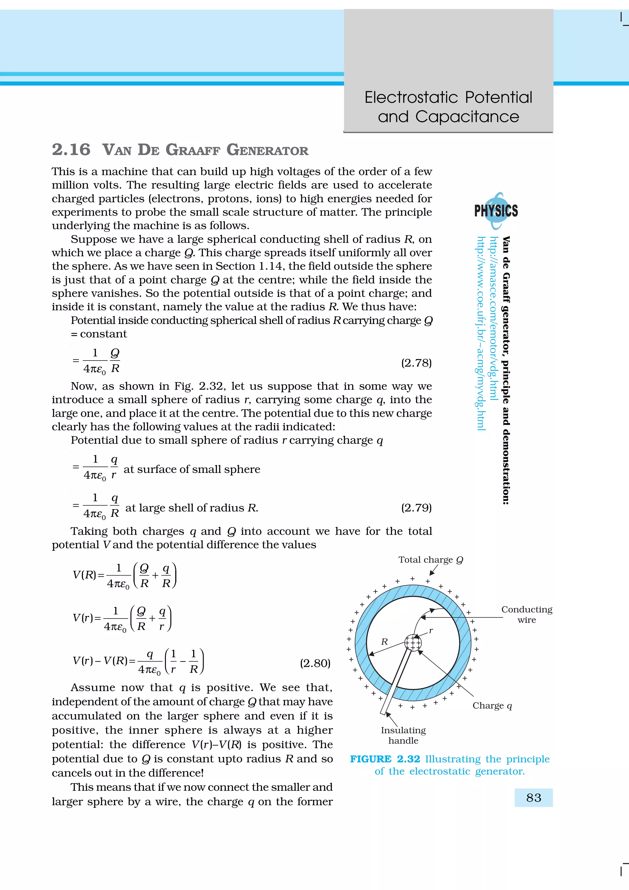
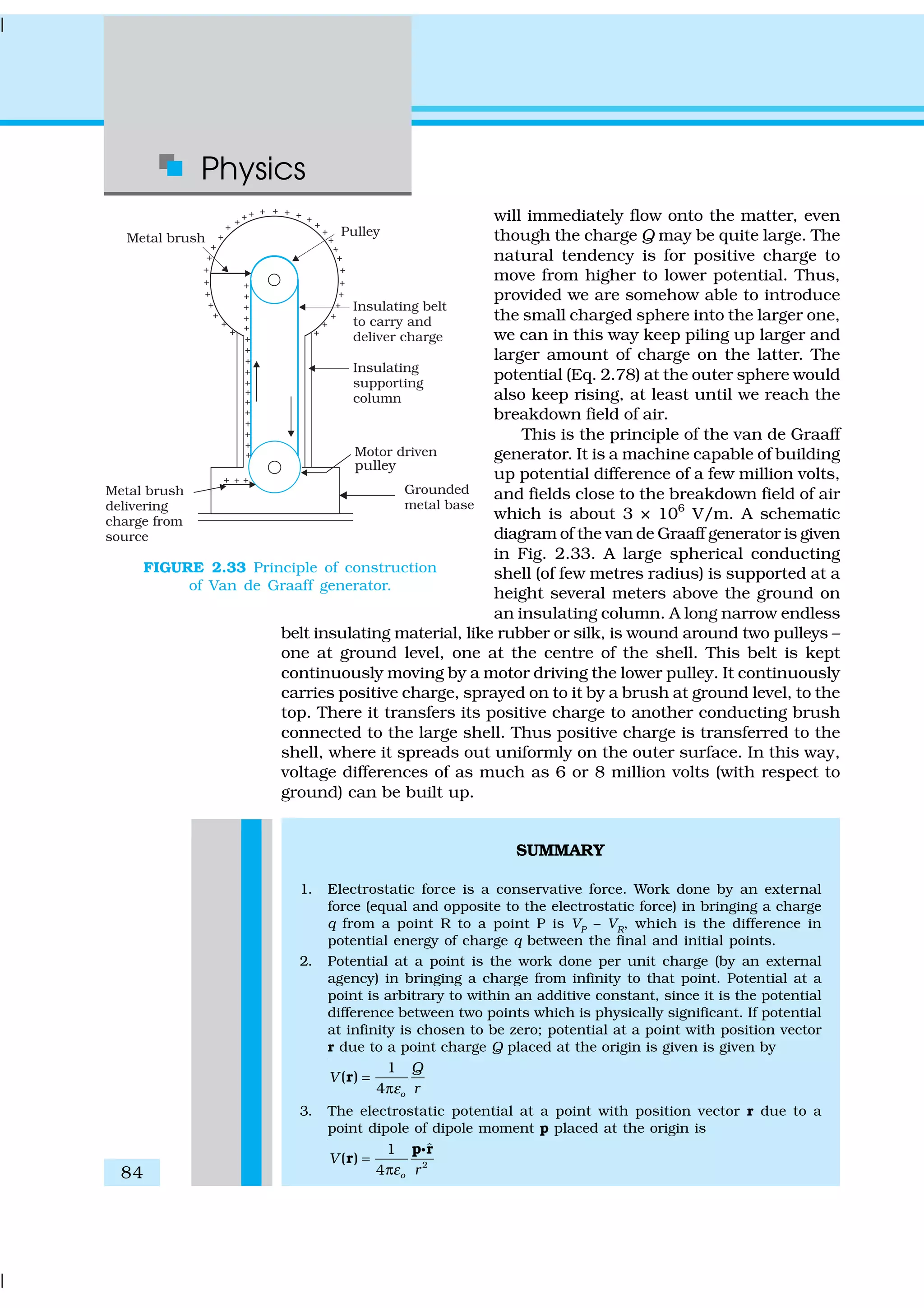
13. A Van de Graaff generator consists of a large spherical conducting shell
(a few metre in diameter). By means of a moving belt and suitable brushes,
charge is continuously transferred to the shell and potential difference
of the order of several million volts is built up, which can be used for
accelerating charged particles.
Physical quantity Symbol Dimensions Unit Remark
Potential φ or V [M1
L2
T–3
A–1
] V Potential difference is
physically significant
Capacitance C [M–1
L–2
T–4
A2
] F
Polarisation P [L–2
AT] C m-2
Dipole moment per unit
volume
Dielectric constant K [Dimensionless]
POINTS TO PONDER
1. Electrostatics deals with forces between charges at rest. But if there is a
force on a charge, how can it be at rest? Thus, when we are talking of
electrostatic force between charges, it should be understood that each
charge is being kept at rest by some unspecified force that opposes the
net Coulomb force on the charge.
2. A capacitor is so configured that it confines the electric field lines within
a small region of space. Thus, even though field may have considerable
strength, the potential difference between the two conductors of a
capacitor is small.
3. Electric field is discontinuous across the surface of a spherical charged
shell. It is zero inside and 0
ˆσ
ε n outside. Electric potential is, however
continuous across the surface, equal to q/4πε0R at the surface.
4. The torque p × E on a dipole causes it to oscillate about E. Only if there
is a dissipative mechanism, the oscillations are damped and the dipole
eventually aligns with E.

91. Electrostatic Potential
and Capacitance
87
EXERCISES
2.1 Two charges 5 × 10–8
C and –3 × 10–8
C are located 16 cm apart. At
what point(s) on the line joining the two charges is the electric
potential zero? Take the potential at infinity to be zero.
2.2 A regular hexagon of side 10 cm has a charge 5 µC at each of its
vertices. Calculate the potential at the centre of the hexagon.
2.3 Two charges 2 µC and –2 µC are placed at points A and B 6 cm
apart.
(a) Identify an equipotential surface of the system.
(b) What is the direction of the electric field at every point on this
surface?
2.4 A spherical conductor of radius 12 cm has a charge of 1.6 × 10–7
C
distributed uniformly on its surface. What is the electric field
(a) inside the sphere
(b) just outside the sphere
(c) at a point 18 cm from the centre of the sphere?
2.5 A parallel plate capacitor with air between the plates has a
capacitance of 8 pF (1pF = 10–12
F). What will be the capacitance if
the distance between the plates is reduced by half, and the space
between them is filled with a substance of dielectric constant 6?
2.6 Three capacitors each of capacitance 9 pF are connected in series.
(a) What is the total capacitance of the combination?
(b) What is the potential difference across each capacitor if the
combination is connected to a 120 V supply?
2.7 Three capacitors of capacitances 2 pF, 3 pF and 4 pF are connected
in parallel.
(a) What is the total capacitance of the combination?
(b) Determine the charge on each capacitor if the combination is
connected to a 100 V supply.
2.8 In a parallel plate capacitor with air between the plates, each plate
has an area of 6 × 10–3
m2
and the distance between the plates is 3 mm.
Calculate the capacitance of the capacitor. If this capacitor is
connected to a 100 V supply, what is the charge on each plate of
the capacitor?
5. Potential due to a charge q at its own location is not defined – it is
infinite.
6. In the expression qV (r) for potential energy of a charge q, V (r) is the
potential due to external charges and not the potential due to q. As seen
in point 5, this expression will be ill-defined if V (r) includes potential
due to a charge q itself.
7. A cavity inside a conductor is shielded from outside electrical influences.
It is worth noting that electrostatic shielding does not work the other
way round; that is, if you put charges inside the cavity, the exterior of
the conductor is not shielded from the fields by the inside charges.

92. Physics
88
2.9 Explain what would happen if in the capacitor given in Exercise
2.8, a 3 mm thick mica sheet (of dielectric constant = 6) were inserted
between the plates,
(a) while the voltage supply remained connected.
(b) after the supply was disconnected.
2.10 A 12pF capacitor is connected to a 50V battery. How much
electrostatic energy is stored in the capacitor?
2.11 A 600pF capacitor is charged by a 200V supply. It is then
disconnected from the supply and is connected to another
uncharged 600 pF capacitor. How much electrostatic energy is lost
in the process?
ADDITIONAL EXERCISES
2.12 A charge of 8 mC is located at the origin. Calculate the work done in
taking a small charge of –2 × 10–9
C from a point P (0, 0, 3 cm) to a
point Q (0, 4 cm, 0), via a point R (0, 6 cm, 9 cm).
2.13 A cube of side b has a charge q at each of its vertices. Determine the
potential and electric field due to this charge array at the centre of
the cube.
2.14 Two tiny spheres carrying charges 1.5 µC and 2.5 µC are located 30 cm
apart. Find the potential and electric field:
(a) at the mid-point of the line joining the two charges, and
(b) at a point 10 cm from this midpoint in a plane normal to the
line and passing through the mid-point.
2.15 A spherical conducting shell of inner radius r1
and outer radius r2
has a charge Q.
(a) A charge q is placed at the centre of the shell. What is the
surface charge density on the inner and outer surfaces of the
shell?
(b) Is the electric field inside a cavity (with no charge) zero, even if
the shell is not spherical, but has any irregular shape? Explain.
2.16 (a) Show that the normal component of electrostatic field has a
discontinuity from one side of a charged surface to another
given by
2 1
0
ˆ( )
σ
ε
− =E E nC
where ˆn is a unit vector normal to the surface at a point and
σ is the surface charge density at that point. (The direction of
ˆn is from side 1 to side 2.) Hence show that just outside a
conductor, the electric field is σ ˆn /ε0
.
(b) Show that the tangential component of electrostatic field is
continuous from one side of a charged surface to another. [Hint:
For (a), use Gauss’s law. For, (b) use the fact that work done by
electrostatic field on a closed loop is zero.]
2.17 A long charged cylinder of linear charged density λ is surrounded
by a hollow co-axial conducting cylinder. What is the electric field in
the space between the two cylinders?
2.18 In a hydrogen atom, the electron and proton are bound at a distance
of about 0.53 Å:

93. Electrostatic Potential
and Capacitance
89
(a) Estimate the potential energy of the system in eV, taking the
zero of the potential energy at infinite separation of the electron
from proton.
(b) What is the minimum work required to free the electron, given
that its kinetic energy in the orbit is half the magnitude of
potential energy obtained in (a)?
(c) What are the answers to (a) and (b) above if the zero of potential
energy is taken at 1.06 Å separation?
2.19 If one of the two electrons of a H2
molecule is removed, we get a
hydrogen molecular ion H+
2
. In the ground state of an H+
2
, the two
protons are separated by roughly 1.5 Å, and the electron is roughly
1 Å from each proton. Determine the potential energy of the system.
Specify your choice of the zero of potential energy.
2.20 Two charged conducting spheres of radii a and b are connected to
each other by a wire. What is the ratio of electric fields at the surfaces
of the two spheres? Use the result obtained to explain why charge
density on the sharp and pointed ends of a conductor is higher
than on its flatter portions.
2.21 Two charges –q and +q are located at points (0, 0, –a) and (0, 0, a),
respectively.
(a) What is the electrostatic potential at the points (0, 0, z) and
(x, y, 0) ?
(b) Obtain the dependence of potential on the distance r of a point
from the origin when r/a >> 1.
(c) How much work is done in moving a small test charge from the
point (5,0,0) to (–7,0,0) along the x-axis? Does the answer
change if the path of the test charge between the same points
is not along the x-axis?
2.22 Figure 2.34 shows a charge array known as an electric quadrupole.
For a point on the axis of the quadrupole, obtain the dependence
of potential on r for r/a >> 1, and contrast your results with that
due to an electric dipole, and an electric monopole (i.e., a single
charge).
FIGURE 2.34
2.23 An electrical technician requires a capacitance of 2 µF in a circuit
across a potential difference of 1 kV. A large number of 1 µF capacitors
are available to him each of which can withstand a potential
difference of not more than 400 V. Suggest a possible arrangement
that requires the minimum number of capacitors.
2.24 What is the area of the plates of a 2 F parallel plate capacitor, given
that the separation between the plates is 0.5 cm? [You will realise
from your answer why ordinary capacitors are in the range of µF or
less. However, electrolytic capacitors do have a much larger
capacitance (0.1 F) because of very minute separation between the
conductors.]

94. Physics
90
2.25 Obtain the equivalent capacitance of the network in Fig. 2.35. For a
300 V supply, determine the charge and voltage across each capacitor.
FIGURE 2.35
2.26 The plates of a parallel plate capacitor have an area of 90 cm2
each
and are separated by 2.5 mm. The capacitor is charged by connecting
it to a 400 V supply.
(a) How much electrostatic energy is stored by the capacitor?
(b) View this energy as stored in the electrostatic field between
the plates, and obtain the energy per unit volume u. Hence
arrive at a relation between u and the magnitude of electric
field E between the plates.
2.27 A 4 µF capacitor is charged by a 200 V supply. It is then disconnected
from the supply, and is connected to another uncharged 2 µF
capacitor. How much electrostatic energy of the first capacitor is
lost in the form of heat and electromagnetic radiation?
2.28 Show that the force on each plate of a parallel plate capacitor has a
magnitude equal to (½) QE, where Q is the charge on the capacitor,
and E is the magnitude of electric field between the plates. Explain
the origin of the factor ½.
2.29 A spherical capacitor consists of two concentric spherical conductors,
held in position by suitable insulating supports (Fig. 2.36). Show
FIGURE 2.36

95. Electrostatic Potential
and Capacitance
91
that the capacitance of a spherical capacitor is given by
0 1 2
1 2
4
–
r r
C
r r
επ
=
where r1
and r2
are the radii of outer and inner spheres,
respectively.
2.30 A spherical capacitor has an inner sphere of radius 12 cm and an
outer sphere of radius 13 cm. The outer sphere is earthed and the
inner sphere is given a charge of 2.5 µC. The space between the
concentric spheres is filled with a liquid of dielectric constant 32.
(a) Determine the capacitance of the capacitor.
(b) What is the potential of the inner sphere?
(c) Compare the capacitance of this capacitor with that of an
isolated sphere of radius 12 cm. Explain why the latter is much
smaller.
2.31 Answer carefully:
(a) Two large conducting spheres carrying charges Q1
and Q2
are
brought close to each other. Is the magnitude of electrostatic
force between them exactly given by Q1
Q2
/4πε0
r2
, where r is
the distance between their centres?
(b) If Coulomb’s law involved 1/r3
dependence (instead of 1/r2
),
would Gauss’s law be still true ?
(c) A small test charge is released at rest at a point in an
electrostatic field configuration. Will it travel along the field
line passing through that point?
(d) What is the work done by the field of a nucleus in a complete
circular orbit of the electron? What if the orbit is elliptical?
(e) We know that electric field is discontinuous across the surface
of a charged conductor. Is electric potential also discontinuous
there?
(f ) What meaning would you give to the capacitance of a single
conductor?
(g) Guess a possible reason why water has a much greater
dielectric constant (= 80) than say, mica (= 6).
2.32 A cylindrical capacitor has two co-axial cylinders of length 15 cm
and radii 1.5 cm and 1.4 cm. The outer cylinder is earthed and the
inner cylinder is given a charge of 3.5 µC. Determine the capacitance
of the system and the potential of the inner cylinder. Neglect end
effects (i.e., bending of field lines at the ends).
2.33 A parallel plate capacitor is to be designed with a voltage rating
1 kV, using a material of dielectric constant 3 and dielectric strength
about 107
Vm–1
. (Dielectric strength is the maximum electric field a
material can tolerate without breakdown, i.e., without starting to
conduct electricity through partial ionisation.) For safety, we should
like the field never to exceed, say 10% of the dielectric strength.
What minimum area of the plates is required to have a capacitance
of 50 pF?
2.34 Describe schematically the equipotential surfaces corresponding to
(a) a constant electric field in the z-direction,
(b) a field that uniformly increases in magnitude but remains in a
constant (say, z) direction,

96. Physics
92
(c) a single positive charge at the origin, and
(d) a uniform grid consisting of long equally spaced parallel charged
wires in a plane.
2.35 In a Van de Graaff type generator a spherical metal shell is to be a
15 × 106
V electrode. The dielectric strength of the gas surrounding
the electrode is 5 × 107
Vm–1
. What is the minimum radius of the
spherical shell required? (You will learn from this exercise why one
cannot build an electrostatic generator using a very small shell
which requires a small charge to acquire a high potential.)
2.36 A small sphere of radius r1
and charge q1
is enclosed by a spherical
shell of radius r2
and charge q2
. Show that if q1
is positive, charge
will necessarily flow from the sphere to the shell (when the two are
connected by a wire) no matter what the charge q2
on the shell is.
2.37 Answer the following:
(a) The top of the atmosphere is at about 400 kV with respect to
the surface of the earth, corresponding to an electric field that
decreases with altitude. Near the surface of the earth, the field
is about 100 Vm–1
. Why then do we not get an electric shock as
we step out of our house into the open? (Assume the house to
be a steel cage so there is no field inside!)
(b) A man fixes outside his house one evening a two metre high
insulating slab carrying on its top a large aluminium sheet of
area 1m2
. Will he get an electric shock if he touches the metal
sheet next morning?
(c) The discharging current in the atmosphere due to the small
conductivity of air is known to be 1800 A on an average over
the globe. Why then does the atmosphere not discharge itself
completely in due course and become electrically neutral? In
other words, what keeps the atmosphere charged?
(d) What are the forms of energy into which the electrical energy
of the atmosphere is dissipated during a lightning?
(Hint: The earth has an electric field of about 100 Vm–1
at its
surface in the downward direction, corresponding to a surface
charge density = –10–9
C m–2
. Due to the slight conductivity of
the atmosphere up to about 50 km (beyond which it is good
conductor), about + 1800 C is pumped every second into the
earth as a whole. The earth, however, does not get discharged
since thunderstorms and lightning occurring continually all
over the globe pump an equal amount of negative charge on
the earth.)

97. 3.1 INTRODUCTION
In Chapter 1, all charges whether free or bound, were considered to be at
rest. Charges in motion constitute an electric current. Such currents occur
naturally in many situations. Lightning is one such phenomenon in
which charges flow from the clouds to the earth through the atmosphere,
sometimes with disastrous results. The flow of charges in lightning is not
steady, but in our everyday life we see many devices where charges flow
in a steady manner, like water flowing smoothly in a river. A torch and a
cell-driven clock are examples of such devices. In the present chapter, we
shall study some of the basic laws concerning steady electric currents.
3.2 ELECTRIC CURRENT
Imagine a small area held normal to the direction of flow of charges. Both
the positive and the negative charges may flow forward and backward
across the area. In a given time interval t, let q+
be the net amount (i.e.,
forward minus backward) of positive charge that flows in the forward
direction across the area. Similarly, let q–
be the net amount of negative
charge flowing across the area in the forward direction. The net amount
of charge flowing across the area in the forward direction in the time
interval t, then, is q = q+– q–. This is proportional to t for steady current
Chapter Three
CURRENT
ELECTRICITY

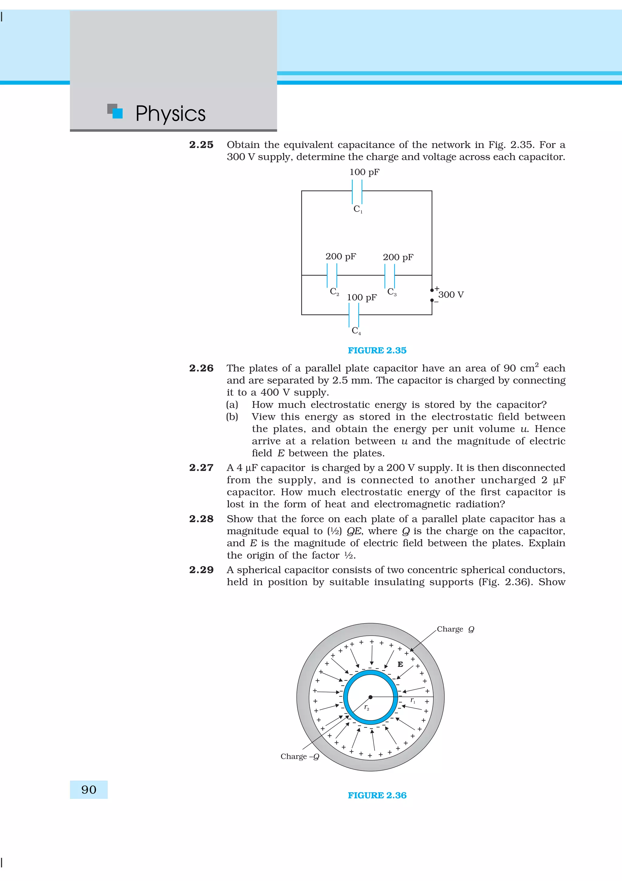
98. Physics
94
and the quotient
q
I
t
= (3.1)
is defined to be the current across the area in the forward direction. (If it
turn out to be a negative number, it implies a current in the backward
direction.)
Currents are not always steady and hence more generally, we define
the current as follows. Let ∆Q be the net charge flowing across a cross-
section of a conductor during the time interval ∆t [i.e., between times t
and (t + ∆t)]. Then, the current at time t across the cross-section of the
conductor is defined as the value of the ratio of ∆Q to ∆t in the limit of ∆t
tending to zero,
( ) 0
lim
t
Q
I t
t∆ →
∆
≡
∆
(3.2)
In SI units, the unit of current is ampere. An ampere is defined
through magnetic effects of currents that we will study in the following
chapter. An ampere is typically the order of magnitude of currents in
domestic appliances. An average lightning carries currents of the order
of tens of thousands of amperes and at the other extreme, currents in
our nerves are in microamperes.
3.3 ELECTRIC CURRENTS IN CONDUCTORS
An electric charge will experience a force if an electric field is applied. If it is
free to move, it will thus move contributing to a current. In nature, free
charged particles do exist like in upper strata of atmosphere called the
ionosphere. However, in atoms and molecules, the negatively charged
electrons and the positively charged nuclei are bound to each other and
are thus not free to move. Bulk matter is made up of many molecules, a
gram of water, for example, contains approximately 1022
molecules. These
molecules are so closely packed that the electrons are no longer attached
to individual nuclei. In some materials, the electrons will still be bound,
i.e., they will not accelerate even if an electric field is applied. In other
materials, notably metals, some of the electrons are practically free to move
within the bulk material. These materials, generally called conductors,
develop electric currents in them when an electric field is applied.
If we consider solid conductors, then of course the atoms are tightly
bound to each other so that the current is carried by the negatively
charged electrons. There are, however, other types of conductors like
electrolytic solutions where positive and negative charges both can move.
In our discussions, we will focus only on solid conductors so that the
current is carried by the negatively charged electrons in the background
of fixed positive ions.
Consider first the case when no electric field is present. The electrons
will be moving due to thermal motion during which they collide with the
fixed ions. An electron colliding with an ion emerges with the same speed
as before the collision. However, the direction of its velocity after the
collision is completely random. At a given time, there is no preferential
direction for the velocities of the electrons. Thus on the average, the

99. Current
Electricity
95
number of electrons travelling in any direction will be equal to the number
of electrons travelling in the opposite direction. So, there will be no net
electric current.
Let us now see what happens to such a
piece of conductor if an electric field is applied.
To focus our thoughts, imagine the conductor
in the shape of a cylinder of radius R (Fig. 3.1).
Suppose we now take two thin circular discs
of a dielectric of the same radius and put
positive charge +Q distributed over one disc
and similarly –Q at the other disc. We attach
the two discs on the two flat surfaces of the
cylinder. An electric field will be created and
is directed from the positive towards the
negative charge. The electrons will be accelerated due to this field towards
+Q. They will thus move to neutralise the charges. The electrons, as long
as they are moving, will constitute an electric current. Hence in the
situation considered, there will be a current for a very short while and no
current thereafter.
We can also imagine a mechanism where the ends of the cylinder are
supplied with fresh charges to make up for any charges neutralised by
electrons moving inside the conductor. In that case, there will be a steady
electric field in the body of the conductor. This will result in a continuous
current rather than a current for a short period of time. Mechanisms,
which maintain a steady electric field are cells or batteries that we shall
study later in this chapter. In the next sections, we shall study the steady
current that results from a steady electric field in conductors.
3.4 OHM’S LAW
A basic law regarding flow of currents was discovered by G.S. Ohm in
1828, long before the physical mechanism responsible for flow of currents
was discovered. Imagine a conductor through which a current I is flowing
and let V be the potential difference between the ends of the conductor.
Then Ohm’s law states that
V ∝ I
or, V = R I (3.3)
where the constant of proportionality R is called the resistance of the
conductor. The SI units of resistance is ohm, and is denoted by the symbol
Ω. The resistance R not only depends on the material of the conductor
but also on the dimensions of the conductor. The dependence of R on the
dimensions of the conductor can easily be determined as follows.
Consider a conductor satisfying Eq. (3.3) to be in the form of a slab of
length l and cross sectional area A [Fig. 3.2(a)]. Imagine placing two such
identical slabs side by side [Fig. 3.2(b)], so that the length of the
combination is 2l. The current flowing through the combination is the
same as that flowing through either of the slabs. If V is the potential
difference across the ends of the first slab, then V is also the potential
difference across the ends of the second slab since the second slab is
FIGURE 3.1 Charges +Q and –Q put at the ends
of a metallic cylinder. The electrons will drift
because of the electric field created to
neutralise the charges. The current thus
will stop after a while unless the charges +Q
and –Q are continuously replenished.
FIGURE 3.2
Illustrating the
relation R = ρl/A for
a rectangular slab
of length l and area
of cross-section A.

100. Physics
96
identical to the first and the same current I flows through
both. The potential difference across the ends of the
combination is clearly sum of the potential difference
across the two individual slabs and hence equals 2V. The
current through the combination is I and the resistance
of the combination RC is [from Eq. (3.3)],
2
2C
V
R R
I
= = (3.4)
since V/I = R, the resistance of either of the slabs. Thus,
doubling the length of a conductor doubles the
resistance. In general, then resistance is proportional to
length,
R l∝ (3.5)
Next, imagine dividing the slab into two by cutting it
lengthwise so that the slab can be considered as a
combination of two identical slabs of length l, but each
having a cross sectional area of A/2 [Fig. 3.2(c)].
For a given voltage V across the slab, if I is the current
through the entire slab, then clearly the current flowing
through each of the two half-slabs is I/2. Since the
potential difference across the ends of the half-slabs is V,
i.e., the same as across the full slab, the resistance of each
of the half-slabs R1
is
1 2 2 .
( /2)
V V
R R
I I
= = = (3.6)
Thus, halving the area of the cross-section of a conductor doubles
the resistance. In general, then the resistance R is inversely proportional
to the cross-sectional area,
1
R
A
∝ (3.7)
Combining Eqs. (3.5) and (3.7), we have
l
R
A
∝ (3.8)
and hence for a given conductor
l
R
A
ρ= (3.9)
where the constant of proportionality ρ depends on the material of the
conductor but not on its dimensions. ρ is called resistivity.
Using the last equation, Ohm’s law reads
I l
V I R
A
ρ
= × = (3.10)
Current per unit area (taken normal to the current), I/A, is called
current density and is denoted by j. The SI units of the current density
are A/m2
. Further, if E is the magnitude of uniform electric field in the
conductor whose length is l, then the potential difference V across its
ends is El. Using these, the last equation reads
GEORGSIMONOHM(1787–1854)
Georg Simon Ohm (1787–
1854) German physicist,
professor at Munich. Ohm
was led to his law by an
analogy between the
conduction of heat: the
electric field is analogous to
the temperature gradient,
and the electric current is
analogous to the heat flow.

101. Current
Electricity
97
E l = j ρ l
or, E = j ρ (3.11)
The above relation for magnitudes E and j can indeed be cast in a
vector form. The current density, (which we have defined as the current
through unit area normal to the current) is also directed along E, and is
also a vector j (≡ j E/E). Thus, the last equation can be written as,
E = jρ (3.12)
or, j = σ E (3.13)
where σ ≡1/ρ is called the conductivity. Ohm’s law is often stated in an
equivalent form, Eq. (3.13) in addition to Eq.(3.3). In the next section, we
will try to understand the origin of the Ohm’s law as arising from the
characteristics of the drift of electrons.
3.5 DRIFT OF ELECTRONS AND THE ORIGIN OF
RESISTIVITY
As remarked before, an electron will suffer collisions with the heavy fixed
ions, but after collision, it will emerge with the same speed but in random
directions. If we consider all the electrons, their average velocity will be
zero since their directions are random. Thus, if there are N electrons and
the velocity of the ith
electron (i = 1, 2, 3, ... N) at a given time is vi
, then
1
1
0
N
i
iN =
=∑v (3.14)
Consider now the situation when an electric field is
present. Electrons will be accelerated due to this
field by
–e
m
=
E
a (3.15)
where –e is the charge and m is the mass of an electron.
Consider again the ith
electron at a given time t. This
electron would have had its last collision some time
before t, and let ti be the time elapsed after its last
collision. If vi
was its velocity immediately after the last
collision, then its velocity Vi
at time t is
–i i i
e
t
m
=
E
V v (3.16)
since starting with its last collision it was accelerated
(Fig. 3.3) with an acceleration given by Eq. (3.15) for a
time interval ti
. The average velocity of the electrons at
time t is the average of all the Vi’s. The average of vi’s is
zero [Eq. (3.14)] since immediately after any collision,
the direction of the velocity of an electron is completely
random. The collisions of the electrons do not occur at
regular intervals but at random times. Let us denote by
τ, the average time between successive collisions. Then
at a given time, some of the electrons would have spent
FIGURE 3.3 A schematic picture of
an electron moving from a point A to
another point B through repeated
collisions, and straight line travel
between collisions (full lines). If an
electric field is applied as shown, the
electron ends up at point B′ (dotted
lines). A slight drift in a direction
opposite the electric field is visible.

102. Physics
98
time more than τ and some less than τ. In other words, the time ti
in
Eq. (3.16) will be less than τ for some and more than τ for others as we go
through the values of i = 1, 2 ..... N. The average value of ti then is τ
(known as relaxation time). Thus, averaging Eq. (3.16) over the
N-electrons at any given time t gives us for the average velocity vd
( ) ( ) ( )d i i iaverage average average
e
t
m
≡ = −
E
v V v
0 –
e e
m m
τ τ= = −
E E
(3.17)
This last result is surprising. It tells us that the
electrons move with an average velocity which is
independent of time, although electrons are
accelerated. This is the phenomenon of drift and the
velocity vd in Eq. (3.17) is called the drift velocity.
Because of the drift, there will be net transport of
charges across any area perpendicular to E. Consider
a planar area A, located inside the conductor such that
the normal to the area is parallel to E
(Fig. 3.4). Then because of the drift, in an infinitesimal
amount of time ∆t, all electrons to the left of the area at
distances upto |vd
|∆t would have crossed the area. If
n is the number of free electrons per unit volume in
the metal, then there are n ∆t |vd|A such electrons.
Since each electron carries a charge –e, the total charge transported across
this area A to the right in time ∆t is –ne A|vd
|∆t. E is directed towards the
left and hence the total charge transported along E across the area is
negative of this. The amount of charge crossing the area A in time ∆t is by
definition [Eq. (3.2)] I ∆t, where I is the magnitude of the current. Hence,
dI t n e A t∆ = + ∆v (3.18)
Substituting the value of |vd| from Eq. (3.17)
2
e A
I t n t
m
τ∆ = ∆ E (3.19)
By definition I is related to the magnitude |j| of the current density by
I = |j|A (3.20)
Hence, from Eqs.(3.19) and (3.20),
2
ne
m
τ=j E (3.21)
The vector j is parallel to E and hence we can write Eq. (3.21) in the
vector form
2
ne
m
τ=j E (3.22)
Comparison with Eq. (3.13) shows that Eq. (3.22) is exactly the Ohm’s
law, if we identify the conductivity σ as
FIGURE 3.4 Current in a metallic
conductor. The magnitude of current
density in a metal is the magnitude of
charge contained in a cylinder of unit
area and length vd
.

103. Current
Electricity
99
EXAMPLE3.1
2
ne
m
σ τ= (3.23)
We thus see that a very simple picture of electrical conduction
reproduces Ohm’s law. We have, of course, made assumptions that τ
and n are constants, independent of E. We shall, in the next section,
discuss the limitations of Ohm’s law.
Example 3.1 (a) Estimate the average drift speed of conduction
electrons in a copper wire of cross-sectional area 1.0 × 10–7
m2
carrying
a current of 1.5 A. Assume that each copper atom contributes roughly
one conduction electron. The density of copper is 9.0 × 103
kg/m3
,
and its atomic mass is 63.5 u. (b) Compare the drift speed obtained
above with, (i) thermal speeds of copper atoms at ordinary
temperatures, (ii) speed of propagation of electric field along the
conductor which causes the drift motion.
Solution
(a) The direction of drift velocity of conduction electrons is opposite
to the electric field direction, i.e., electrons drift in the direction
of increasing potential. The drift speed vd
is given by Eq. (3.18)
vd
= (I/neA)
Now, e = 1.6 × 10–19
C, A = 1.0 × 10–7
m2
, I = 1.5 A. The density of
conduction electrons, n is equal to the number of atoms per cubic
metre (assuming one conduction electron per Cu atom as is
reasonable from its valence electron count of one). A cubic metre
of copper has a mass of 9.0 × 103
kg. Since 6.0 × 1023
copper
atoms have a mass of 63.5 g,
23
66.0 10
9.0 10
63.5
n
×
= × ×
= 8.5 × 1028
m–3
which gives,
28 –19 –7
1.5
8.5 10 1.6 10 1.0 10
=
× × × × ×
dv
= 1.1 × 10–3
m s–1
= 1.1 mm s–1
(b) (i) At a temperature T, the thermal speed* of a copper atom of
mass M is obtained from [<(1/2) Mv2
> = (3/2) kB
T ] and is thus
typically of the order of /Bk T M , where kB
is the Boltzmann
constant. For copper at 300 K, this is about 2 × 102
m/s. This
figure indicates the random vibrational speeds of copper atoms
in a conductor. Note that the drift speed of electrons is much
smaller, about 10–5
times the typical thermal speed at ordinary
temperatures.
(ii) An electric field travelling along the conductor has a speed of
an electromagnetic wave, namely equal to 3.0 × 108
m s–1
(You will learn about this in Chapter 8). The drift speed is, in
comparison, extremely small; smaller by a factor of 10–11
.
* See Eq. (13.23) of Chapter 13 from Class XI book.

104. Physics
100
EXAMPLE3.2
Example 3.2
(a) In Example 3.1, the electron drift speed is estimated to be only a
few mm s–1
for currents in the range of a few amperes? How then
is current established almost the instant a circuit is closed?
(b) The electron drift arises due to the force experienced by electrons
in the electric field inside the conductor. But force should cause
acceleration. Why then do the electrons acquire a steady average
drift speed?
(c) If the electron drift speed is so small, and the electron’s charge is
small, how can we still obtain large amounts of current in a
conductor?
(d) When electrons drift in a metal from lower to higher potential,
does it mean that all the ‘free’ electrons of the metal are moving
in the same direction?
(e) Are the paths of electrons straight lines between successive
collisions (with the positive ions of the metal) in the (i) absence of
electric field, (ii) presence of electric field?
Solution
(a) Electric field is established throughout the circuit, almost instantly
(with the speed of light) causing at every point a local electron
drift. Establishment of a current does not have to wait for electrons
from one end of the conductor travelling to the other end. However,
it does take a little while for the current to reach its steady value.
(b) Each ‘free’ electron does accelerate, increasing its drift speed until
it collides with a positive ion of the metal. It loses its drift speed
after collision but starts to accelerate and increases its drift speed
again only to suffer a collision again and so on. On the average,
therefore, electrons acquire only a drift speed.
(c) Simple, because the electron number density is enormous,
~1029
m–3
.
(d) By no means. The drift velocity is superposed over the large
random velocities of electrons.
(e) In the absence of electric field, the paths are straight lines; in the
presence of electric field, the paths are, in general, curved.
3.5.1 Mobility
As we have seen, conductivity arises from mobile charge carriers. In
metals, these mobile charge carriers are electrons; in an ionised gas, they
are electrons and positive charged ions; in an electrolyte, these can be
both positive and negative ions.
An important quantity is the mobility µ defined as the magnitude of
the drift velocity per unit electric field:
| |d
E
µ =
v
(3.24)
The SI unit of mobility is m2
/Vs and is 104
of the mobility in practical
units (cm2
/Vs). Mobility is positive. From Eq. (3.17), we have
vd =
e E
m
τ

105. Current
Electricity
101
Hence,
dv e
E m
τ
µ = = (3.25)
where τ is the average collision time for electrons.
3.6 LIMITATIONS OF OHM’S LAW
Although Ohm’s law has been found valid over a large class
of materials, there do exist materials and devices used in
electric circuits where the proportionality of V and I does not
hold. The deviations broadly are one or more of the following
types:
(a) V ceases to be proportional to I (Fig. 3.5).
(b) The relation between V and I depends on the sign of V. In
other words, if I is the current for a certain V, then reversing
the direction of V keeping its magnitude fixed, does not
produce a current of the same magnitude as I in the opposite direction
(Fig. 3.6). This happens, for example, in a diode which we will study
in Chapter 14.
(c) The relation between V and I is not unique, i.e., there is more than
one value of V for the same current I (Fig. 3.7). A material exhibiting
such behaviour is GaAs.
Materials and devices not obeying Ohm’s law in the form of Eq. (3.3)
are actually widely used in electronic circuits. In this and a few
subsequent chapters, however, we will study the electrical currents in
materials that obey Ohm’s law.
3.7 RESISTIVITY OF VARIOUS MATERIALS
The resistivities of various common materials are listed in Table 3.1. The
materials are classified as conductors, semiconductors and insulators
FIGURE 3.5 The dashed line
represents the linear Ohm’s
law. The solid line is the voltage
V versus current I for a good
conductor.
FIGURE 3.6 Characteristic curve
of a diode. Note the different
scales for negative and positive
values of the voltage and current.
FIGURE 3.7 Variation of current
versus voltage for GaAs.

106. Physics
102
depending on their resistivities, in an increasing order of their values.
Metals have low resistivities in the range of 10–8
Ωm to 10–6
Ωm. At the
other end are insulators like ceramic, rubber and plastics having
resistivities 1018
times greater than metals or more. In between the two
are the semiconductors. These, however, have resistivities
characteristically decreasing with a rise in temperature. The resistivities
of semiconductors are also affected by presence of small amount of
impurities. This last feature is exploited in use of semiconductors for
electronic devices.
TABLE 3.1 RESISTIVITIES OF SOME MATERIALS
Material Resistivity, ρ Temperature coefficient
(Ω m) at 0°C of resistivity, α (°C) –1
1 d
at 0 C
dT
ρ
ρ
 
°  
Conductors
Silver 1.6 × 10–8
0.0041
Copper 1.7 × 10–8
0.0068
Aluminium 2.7 × 10–8
0.0043
Tungsten 5.6 × 10–8
0.0045
Iron 10 × 10–8
0.0065
Platinum 11 × 10–8
0.0039
Mercury 98 × 10–8
0.0009
Nichrome ~100 × 10–8
0.0004
(alloy of Ni, Fe, Cr)
Manganin (alloy) 48 × 10–8
0.002 × 10–3
Semiconductors
Carbon (graphite) 3.5 × 10–5
– 0.0005
Germanium 0.46 – 0.05
Silicon 2300 – 0.07
Insulators
Pure Water 2.5 × 105
Glass 1010
– 1014
Hard Rubber 1013
– 1016
NaCl ~1014
Fused Quartz ~1016
Commercially produced resistors for domestic use or in laboratories
are of two major types: wire bound resistors and carbon resistors. Wire
bound resistors are made by winding the wires of an alloy, viz., manganin,
constantan, nichrome or similar ones. The choice of these materials is
dictated mostly by the fact that their resistivities are relatively insensitive
to temperature. These resistances are typically in the range of a fraction
of an ohm to a few hundred ohms.

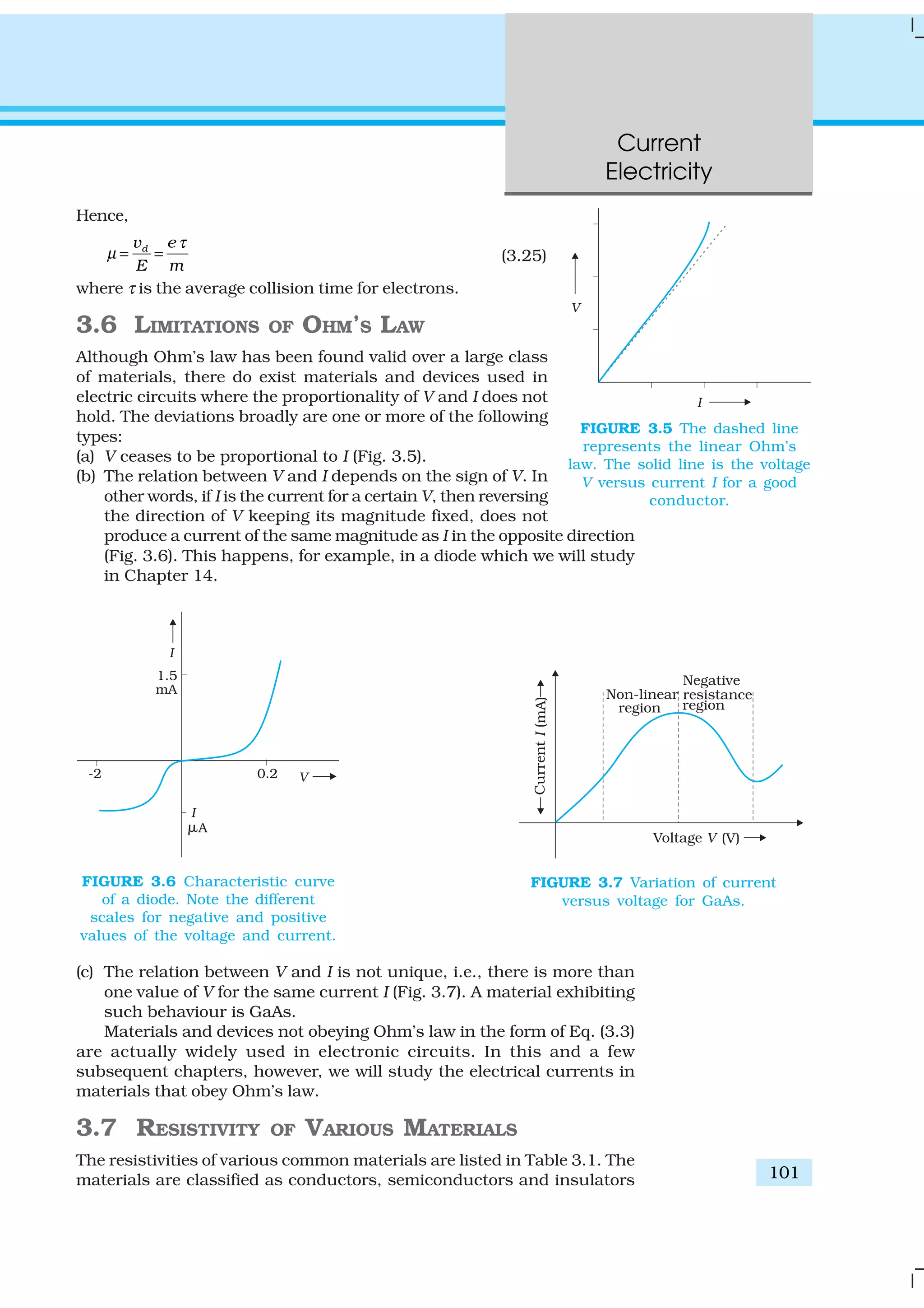
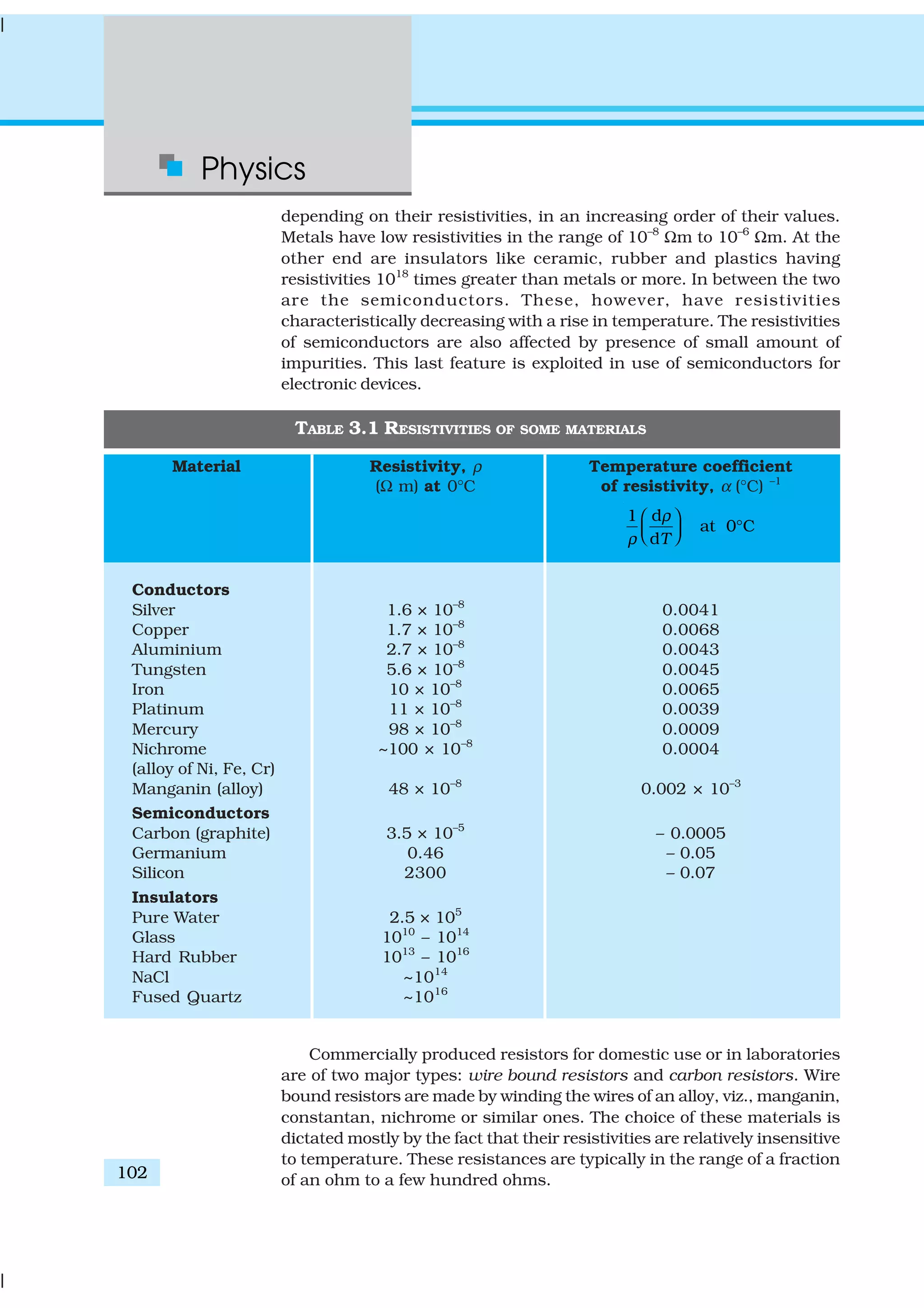
107. Current
Electricity
103
Resistors in the higher range are made mostly from carbon. Carbon
resistors are compact, inexpensive and thus find extensive use in electronic
circuits. Carbon resistors are small in size and hence their values are
given using a colour code.
TABLE 3.2 RESISTOR COLOUR CODES
Colour Number Multiplier Tolerance (%)
Black 0 1
Brown 1 101
Red 2 102
Orange 3 103
Yellow 4 104
Green 5 105
Blue 6 106
Violet 7 107
Gray 8 108
White 9 109
Gold 10–1
5
Silver 10–2
10
No colour 20
The resistors have a set of co-axial coloured rings
on them whose significance are listed in Table 3.2. The
first two bands from the end indicate the first two
significant figures of the resistance in ohms. The third
band indicates the decimal multiplier (as listed in Table
3.2). The last band stands for tolerance or possible
variation in percentage about the indicated values.
Sometimes, this last band is absent and that indicates
a tolerance of 20% (Fig. 3.8). For example, if the four
colours are orange, blue, yellow and gold, the resistance
value is 36 × 104
Ω, with a tolerence value of 5%.
3.8 TEMPERATURE DEPENDENCE OF
RESISTIVITY
The resistivity of a material is found to be dependent on
the temperature. Different materials do not exhibit the
same dependence on temperatures. Over a limited range
of temperatures, that is not too large, the resistivity of a
metallic conductor is approximately given by,
ρT
= ρ0
[1 + α (T–T0
)] (3.26)
where ρT is the resistivity at a temperature T and ρ0 is the same at a
reference temperature T0
. α is called the temperature co-efficient of
resistivity, and from Eq. (3.26), the dimension of α is (Temperature)–1
.
FIGURE 3.8 Colour coded resistors
(a) (22 × 102
Ω) ± 10%,
(b) (47 × 10 Ω) ± 5%.

108. Physics
104
For metals, α is positive and values of α for some metals at T0
= 0°C are
listed in Table 3.1.
The relation of Eq. (3.26) implies that a graph of ρT
plotted against T
would be a straight line. At temperatures much lower than 0°C, the graph,
however, deviates considerably from a straight line (Fig. 3.9).
Equation (3.26) thus, can be used approximately over a limited range
of T around any reference temperature T0
, where the graph can be
approximated as a straight line.
Some materials like Nichrome (which is an alloy of nickel, iron and
chromium) exhibit a very weak dependence of resistivity with temperature
(Fig. 3.10). Manganin and constantan have similar properties. These
materials are thus widely used in wire bound standard resistors since
their resistance values would change very little with temperatures.
Unlike metals, the resistivities of semiconductors decrease with
increasing temperatures. A typical dependence is shown in Fig. 3.11.
We can qualitatively understand the temperature dependence of
resistivity, in the light of our derivation of Eq. (3.23). From this equation,
resistivity of a material is given by
2
1 m
n e
ρ
σ τ
= = (3.27)
ρ thus depends inversely both on the number n of free electrons per unit
volume and on the average time τ between collisions. As we increase
temperature, average speed of the electrons, which act as the carriers of
current, increases resulting in more frequent collisions. The average time
of collisions τ, thus decreases with temperature.
In a metal, n is not dependent on temperature to any appreciable
extent and thus the decrease in the value of τ with rise in temperature
causes ρ to increase as we have observed.
For insulators and semiconductors, however, n increases with
temperature. This increase more than compensates any decrease in τ in
Eq.(3.23) so that for such materials, ρ decreases with temperature.
FIGURE 3.9
Resistivity ρT
of
copper as a function
of temperature T.
FIGURE 3.10 Resistivity
ρT
of nichrome as a
function of absolute
temperature T.
FIGURE 3.11
Temperature dependence
of resistivity for a typical
semiconductor.

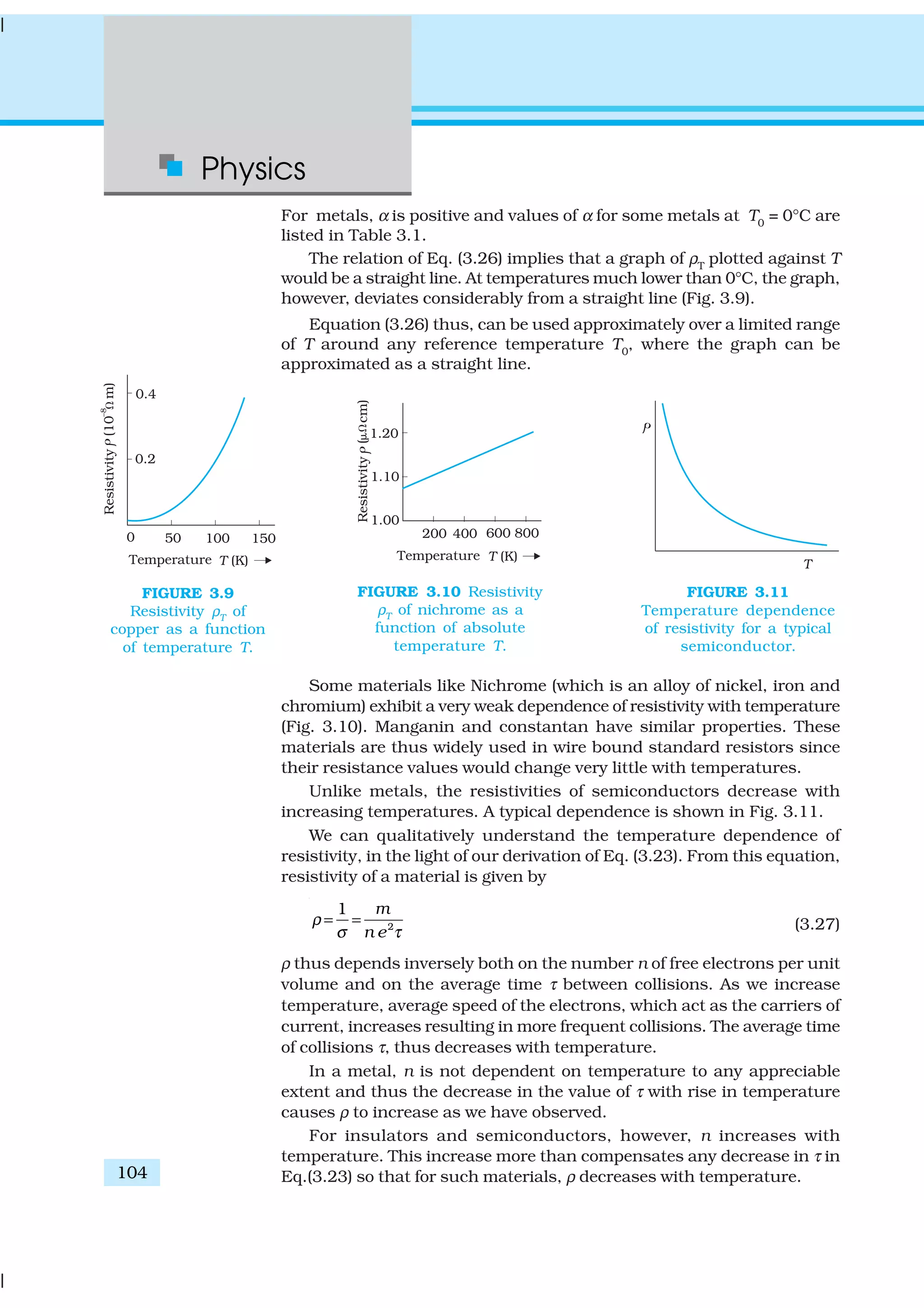
109. Current
Electricity
105
EXAMPLE3.4
Example 3.3 An electric toaster uses nichrome for its heating
element. When a negligibly small current passes through it, its
resistance at room temperature (27.0 °C) is found to be 75.3 Ω. When
the toaster is connected to a 230 V supply, the current settles, after
a few seconds, to a steady value of 2.68 A. What is the steady
temperature of the nichrome element? The temperature coefficient
of resistance of nichrome averaged over the temperature range
involved, is 1.70 × 10–4
°C–1
.
Solution When the current through the element is very small, heating
effects can be ignored and the temperature T1
of the element is the
same as room temperature. When the toaster is connected to the
supply, its initial current will be slightly higher than its steady value
of 2.68 A. But due to heating effect of the current, the temperature
will rise. This will cause an increase in resistance and a slight
decrease in current. In a few seconds, a steady state will be reached
when temperature will rise no further, and both the resistance of the
element and the current drawn will achieve steady values. The
resistance R2
at the steady temperature T2
is
R2
230 V
85.8
2.68 A
= = Ω
Using the relation
R2
= R1
[1 + α (T2
– T1
)]
with α = 1.70 × 10–4
°C–1
, we get
T2
– T1 –4
(85.8 – 75.3)
(75.3) 1.70 10
=
× ×
= 820 °C
that is, T2
= (820 + 27.0) °C = 847 °C
Thus, the steady temperature of the heating element (when heating
effect due to the current equals heat loss to the surroundings) is
847 °C.
Example 3.4 The resistance of the platinum wire of a platinum
resistance thermometer at the ice point is 5 Ω and at steam point is
5.23 Ω. When the thermometer is inserted in a hot bath, the resistance
of the platinum wire is 5.795 Ω. Calculate the temperature of the
bath.
Solution R0
= 5 Ω, R100
= 5.23 Ω and Rt
= 5.795 Ω
Now,
0
0
100 0
100, (1 )t
t
R R
t R R t
R R
α
−
= × = +
−
5.795 5
100
5.23 5
−
= ×
−
=
0.795
100
0.23
× = 345.65 °C
3.9 ELECTRICAL ENERGY, POWER
Consider a conductor with end points A and B, in which a current I is
flowing from A to B. The electric potential at A and B are denoted by V(A)
EXAMPLE3.3

110. Physics
106
and V(B) respectively. Since current is flowing from A to B, V(A) > V(B)
and the potential difference across AB is V = V(A) – V(B) > 0.
In a time interval ∆t, an amount of charge ∆Q = I ∆t travels from A to
B. The potential energy of the charge at A, by definition, was Q V(A) and
similarly at B, it is Q V(B). Thus, change in its potential energy ∆Upot
is
∆Upot = Final potential energy – Initial potential energy
= ∆Q[(V (B) – V (A)] = –∆Q V
= –I V∆t < 0 (3.28)
If charges moved without collisions through the conductor, their
kinetic energy would also change so that the total energy is unchanged.
Conservation of total energy would then imply that,
∆K = –∆Upot
(3.29)
that is,
∆K = I V∆t > 0 (3.30)
Thus, in case charges were moving freely through the conductor under
the action of electric field, their kinetic energy would increase as they
move. We have, however, seen earlier that on the average, charge carriers
do not move with acceleration but with a steady drift velocity. This is
because of the collisions with ions and atoms during transit. During
collisions, the energy gained by the charges thus is shared with the atoms.
The atoms vibrate more vigorously, i.e., the conductor heats up. Thus,
in an actual conductor, an amount of energy dissipated as heat in the
conductor during the time interval ∆t is,
∆W = I V∆t (3.31)
The energy dissipated per unit time is the power dissipated
P = ∆W/∆t and we have,
P = I V (3.32)
Using Ohm’s law V = IR, we get
P = I 2
R = V 2
/R (3.33)
as the power loss (“ohmic loss”) in a conductor of resistance R carrying a
current I. It is this power which heats up, for example, the coil of an
electric bulb to incandescence, radiating out heat and
light.
Where does the power come from? As we have
reasoned before, we need an external source to keep
a steady current through the conductor. It is clearly
this source which must supply this power. In the
simple circuit shown with a cell (Fig.3.12), it is the
chemical energy of the cell which supplies this power
for as long as it can.
The expressions for power, Eqs. (3.32) and (3.33),
show the dependence of the power dissipated in a
resistor R on the current through it and the voltage
across it.
Equation (3.33) has an important application to
power transmission. Electrical power is transmitted
from power stations to homes and factories, which
FIGURE 3.12 Heat is produced in the
resistor R which is connected across
the terminals of a cell. The energy
dissipated in the resistor R comes from
the chemical energy of the electrolyte.

111. Current
Electricity
107
may be hundreds of miles away, via transmission cables. One obviously
wants to minimise the power loss in the transmission cables connecting
the power stations to homes and factories. We shall see now how this
can be achieved. Consider a device R, to which a power P is to be delivered
via transmission cables having a resistance Rc
to be dissipated by it finally.
If V is the voltage across R and I the current through it, then
P = V I (3.34)
The connecting wires from the power station to the device has a finite
resistance Rc. The power dissipated in the connecting wires, which is
wasted is Pc
with
Pc
= I2
Rc
2
2
cP R
V
= (3.35)
from Eq. (3.32). Thus, to drive a device of power P, the power wasted in the
connecting wires is inversely proportional to V 2
. The transmission cables
from power stations are hundreds of miles long and their resistance Rc
is
considerable. To reduce Pc
, these wires carry current at enormous values
of V and this is the reason for the high voltage danger signs on transmission
lines — a common sight as we move away from populated areas. Using
electricity at such voltages is not safe and hence at the other end, a device
called a transformer lowers the voltage to a value suitable for use.
3.10 COMBINATION OF RESISTORS – SERIES AND
PARALLEL
The current through a single resistor R across which there is a potential
difference V is given by Ohm’s law I = V/R. Resistors are sometimes joined
together and there are simple rules for calculation of equivalent resistance
of such combination.
FIGURE 3.13 A series combination of two resistor R1
and R2
.
Two resistors are said to be in series if only one of their end points is
joined (Fig. 3.13). If a third resistor is joined with the series combination
of the two (Fig. 3.14), then all three are said to be in series. Clearly, we
can extend this definition to series combination of any number of resistors.
FIGURE 3.14 A series combination of three resistors R1
, R2
, R3
.
Two or more resistors are said to be in parallel if one end of all the
resistors is joined together and similarly the other ends joined together
(Fig. 3.15).
FIGURE 3.15 Two resistors R1
and R2
connected in parallel.

112. Physics
108
Consider two resistors R1
and R2
in series. The charge which leaves R1
must be entering R2
. Since current measures the rate of flow of charge,
this means that the same current I flows through R1 and R2. By Ohm’s law:
Potential difference across R1 = V1 = I R1, and
Potential difference across R2
= V2
= I R2
.
The potential difference V across the combination is V1+V2. Hence,
V = V1+ V2 = I (R1 + R2) (3.36)
This is as if the combination had an equivalent resistance Req
, which
by Ohm’s law is
Req
V
I
≡ = (R1
+ R2
) (3.37)
If we had three resistors connected in series, then similarly
V = I R1
+ I R2
+ I R3
= I (R1
+ R2
+ R3
). (3.38)
This obviously can be extended to a series combination of any number
n of resistors R1
, R2
....., Rn
. The equivalent resistance Req
is
Req
= R1
+ R2
+ . . . + Rn
(3.39)
Consider now the parallel combination of two resistors (Fig. 3.15).
The charge that flows in at A from the left flows out partly through R1
and partly through R2. The currents I, I1, I2 shown in the figure are the
rates of flow of charge at the points indicated. Hence,
I = I1 + I2 (3.40)
The potential difference between A and B is given by the Ohm’s law
applied to R1
V = I1
R1
(3.41)
Also, Ohm’s law applied to R2 gives
V = I2 R2 (3.42)
∴ I = I1
+ I2
=
1 2 1 2
1 1V V
V
R R R R
 
+ = +  
(3.43)
If the combination was replaced by an equivalent resistance Req
, we
would have, by Ohm’s law
eq
V
I
R
= (3.44)
Hence,
1 2
1 1 1
eqR R R
= + (3.45)
We can easily see how this extends to three resistors in parallel
(Fig. 3.16).
FIGURE 3.16 Parallel combination of three resistors R1
, R2
and R3
.

113. Current
Electricity
109
Exactly as before
I = I1
+ I2
+ I3
(3.46)
and applying Ohm’s law to R1, R2 and R3 we get,
V = I1 R1, V = I2 R2, V = I3 R3 (3.47)
So that
I = I1 + I2 + I3 =
1 2 3
1 1 1
V
R R R
 
+ +  
(3.48)
An equivalent resistance Req
that replaces the combination, would be
such that
eq
V
I
R
= (3.49)
and hence
1 2 3
1 1 1 1
eqR R R R
= + + (3.50)
We can reason similarly for any number of resistors in parallel. The
equivalent resistance of n resistors R1
, R2
. . . ,Rn
is
1 2 n
1 1 1 1
...
eqR R R R
= + + + (3.51)
These formulae for equivalent resistances can be used to find out
currents and voltages in more complicated circuits. Consider for example,
the circuit in Fig. (3.17), where there are three resistors R1, R2 and R3.
R2
and R3
are in parallel and hence we can
replace them by an equivalent
23
eqR between
point B and C with
23
2 3
1 1 1
eq R RR
= +
or,
23 2 3
2 3
Req
R R
R R
=
+ (3.52)
The circuit now has R1
and 23
eqR in series
and hence their combination can be
replaced by an equivalent resistance 123
eqR
with
123 23
1eq eqR R R= + (3.53)
If the voltage between A and C is V, the
current I is given by
( )123
1 2 3 2 3/eq
V V
I
R R R R R R
= =
 + + 
( )2 3
1 2 1 3 2 3
V R R
R R R R R R
+
=
+ +
(3.54)
FIGURE 3.17 A combination of three resistors R1
,
R2
and R3
. R2
, R3
are in parallel with an
equivalent resistance
23
eqR . R1
and
23
eqR are in
series with an equivalent resistance
123
eqR .

114. Physics
110
3.11 CELLS, EMF, INTERNAL RESISTANCE
We have already mentioned that a simple device to maintain a steady
current in an electric circuit is the electrolytic cell. Basically a cell has
two electrodes, called the positive (P) and the negative (N), as shown in
Fig. 3.18. They are immersed in an electrolytic solution. Dipped in the
solution, the electrodes exchange charges with the electrolyte. The
positive electrode has a potential difference V+ (V+ > 0) between
itself and the electrolyte solution immediately adjacent to it marked
A in the figure. Similarly, the negative electrode develops a negative
potential – (V– ) (V– ≥ 0) relative to the electrolyte adjacent to it,
marked as B in the figure. When there is no current, the electrolyte
has the same potential throughout, so that the potential difference
between P and N is V+
– (–V–
) = V+
+ V–
. This difference is called the
electromotive force (emf) of the cell and is denoted by ε. Thus
ε = V+
+V–
> 0 (3.55)
Note that ε is, actually, a potential difference and not a force. The
name emf, however, is used because of historical reasons, and was
given at a time when the phenomenon was not understood properly.
To understand the significance of ε, consider a resistor R
connected across the cell (Fig. 3.18). A current I flows across R
from C to D. As explained before, a steady current is maintained
because current flows from N to P through the electrolyte. Clearly,
across the electrolyte the same current flows through the electrolyte
but from N to P, whereas through R, it flows from P to N.
The electrolyte through which a current flows has a finite
resistance r, called the internal resistance. Consider first the
situation when R is infinite so that I = V/R = 0, where V is the
potential difference between P and N. Now,
V = Potential difference between P and A
+ Potential difference between A and B
+ Potential difference between B and N
= ε (3.56)
Thus, emf ε is the potential difference between the positive and
negative electrodes in an open circuit, i.e., when no current is
flowing through the cell.
If however R is finite, I is not zero. In that case the potential
difference between P and N is
V = V+
+ V–
– I r
= ε – I r (3.57)
Note the negative sign in the expression (I r) for the potential difference
between A and B. This is because the current I flows from B to A in the
electrolyte.
In practical calculations, internal resistances of cells in the circuit
may be neglected when the current I is such that ε >> I r. The actual
values of the internal resistances of cells vary from cell to cell. The internal
resistance of dry cells, however, is much higher than the common
electrolytic cells.
FIGURE 3.18 (a) Sketch of
an electrolyte cell with
positive terminal P and
negative terminal N. The
gap between the electrodes
is exaggerated for clarity. A
and B are points in the
electrolyte typically close to
P and N. (b) the symbol for
a cell, + referring to P and
– referring to the N
electrode. Electrical
connections to the cell are
made at P and N.

115. Current
Electricity
111
We also observe that since V is the potential difference across R, we
have from Ohm’s law
V = I R (3.58)
Combining Eqs. (3.57) and (3.58), we get
I R = ε – I r
Or, I
R r
ε
=
+
(3.59)
The maximum current that can be drawn from a cell is for R = 0 and
it is Imax
= ε/r. However, in most cells the maximum allowed current is
much lower than this to prevent permanent damage to the cell.
CHARGES IN CLOUDS
In olden days lightning was considered as an atmospheric flash of supernatural origin.
It was believed to be the great weapon of Gods. But today the phenomenon of lightning
can be explained scientifically by elementary principles of physics.
Atmospheric electricity arises due to the separation of electric charges. In the
ionosphere and magnetosphere strong electric current is generated from the solar-
terrestrial interaction. In the lower atmosphere the current is weaker and is maintained
by thunderstorm.
There are ice particles in the clouds, which grow, collide, fracture and break apart.
The smaller particles acquire positive charge and the larger ones negative charge. These
charged particles get separated by updrafts in the clouds and gravity. The upper portion
of the cloud becomes positively charged and the middle negatively charged, leading to
dipole structure. Sometimes a very weak positive charge is found near the base of the
cloud. The ground is positively charged at the time of thunderstorm development. Also
cosmic and radioactive radiations ionise air into positive and negative ions and air becomes
(weakly) electrically conductive. The separation of charges produce tremendous amount
of electrical potential within the cloud as well as between the cloud and ground. This can
amount to millions of volts and eventually the electrical resistance in the air breaks
down and lightning flash begins and thousands of amperes of current flows. The electric
field is of the order of 105
V/m. A lightning flash is composed of a series of strokes with
an average of about four and the duration of each flash is about 30 seconds. The average
peak power per stroke is about 1012
watts.
During fair weather also there is charge in the atmosphere. The fair weather electric
field arises due to the existence of a surface charge density at ground and an atmospheric
conductivity as well as due to the flow of current from the ionosphere to the earth’s
surface, which is of the order of picoampere / square metre. The surface charge density
at ground is negative; the electric field is directed downward. Over land the average
electric field is about 120 V/m, which corresponds to a surface charge density of
–1.2 × 10–9
C/m2
. Over the entire earth’s surface, the total negative charge amount to
about 600 kC. An equal positive charge exists in the atmosphere. This electric field is not
noticeable in daily life. The reason why it is not noticed is that virtually everything, including
our bodies, is conductor compared to air.

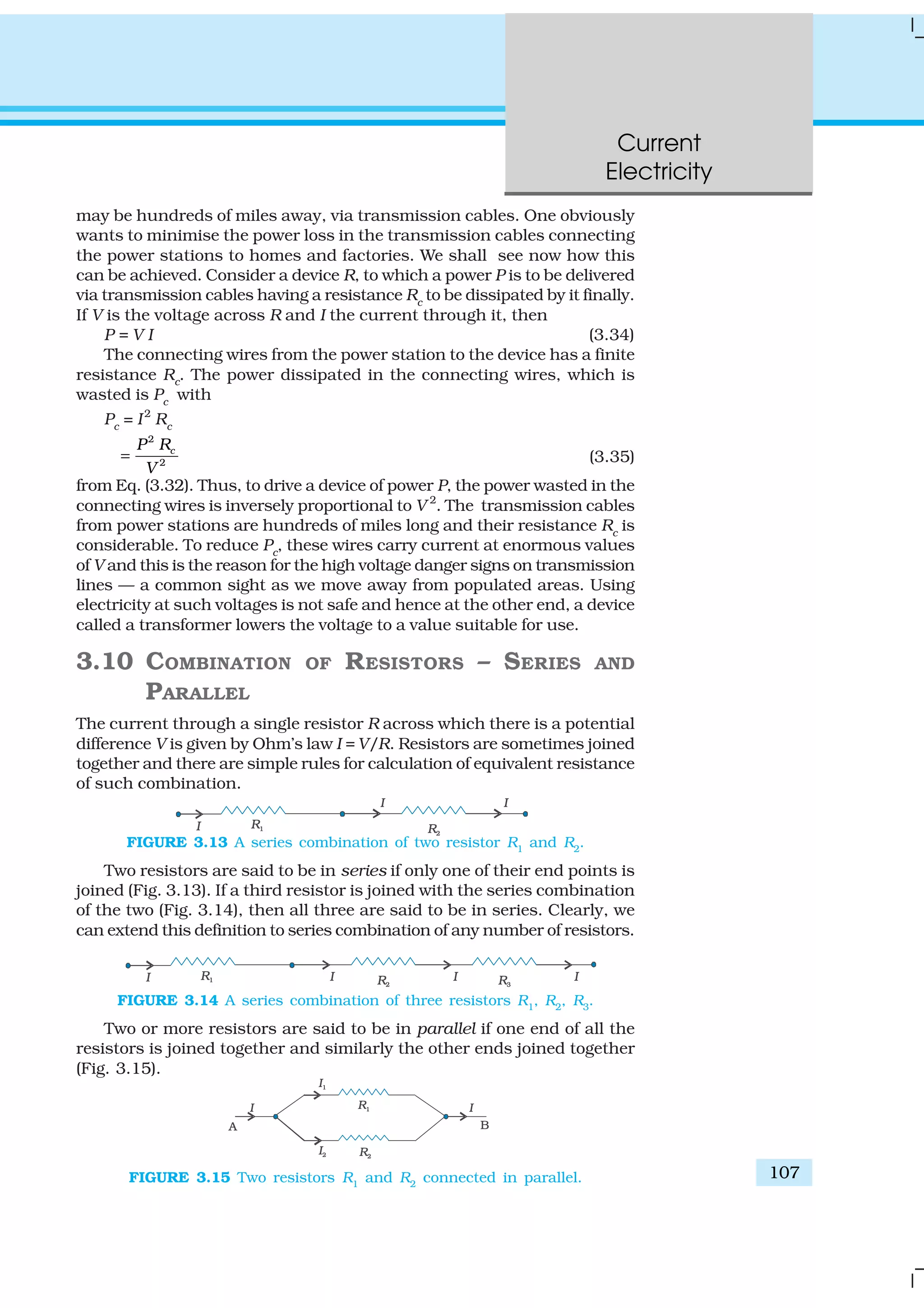
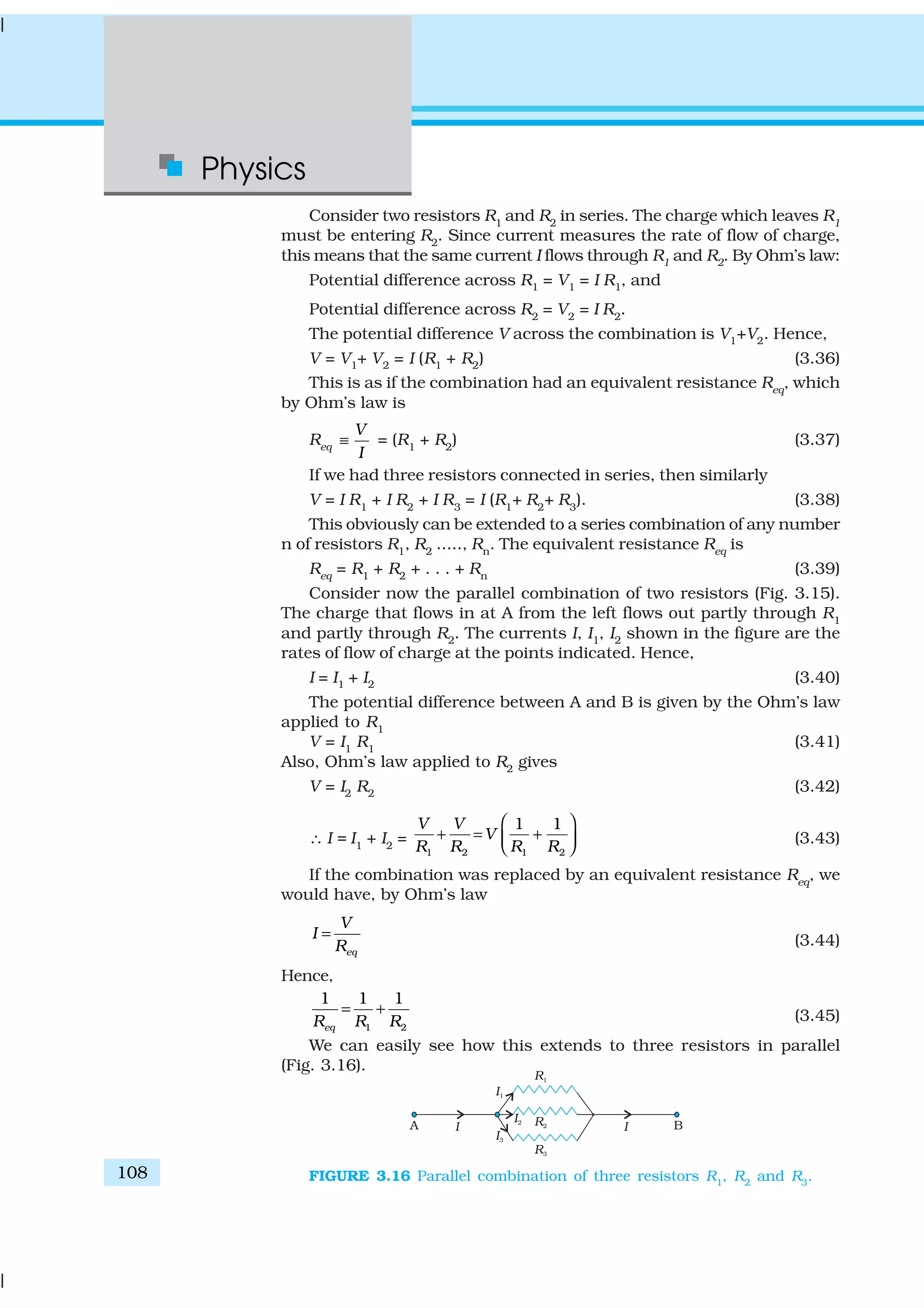
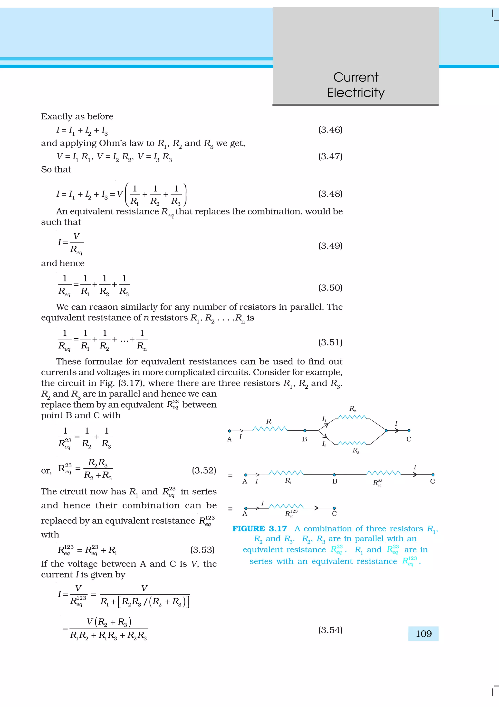
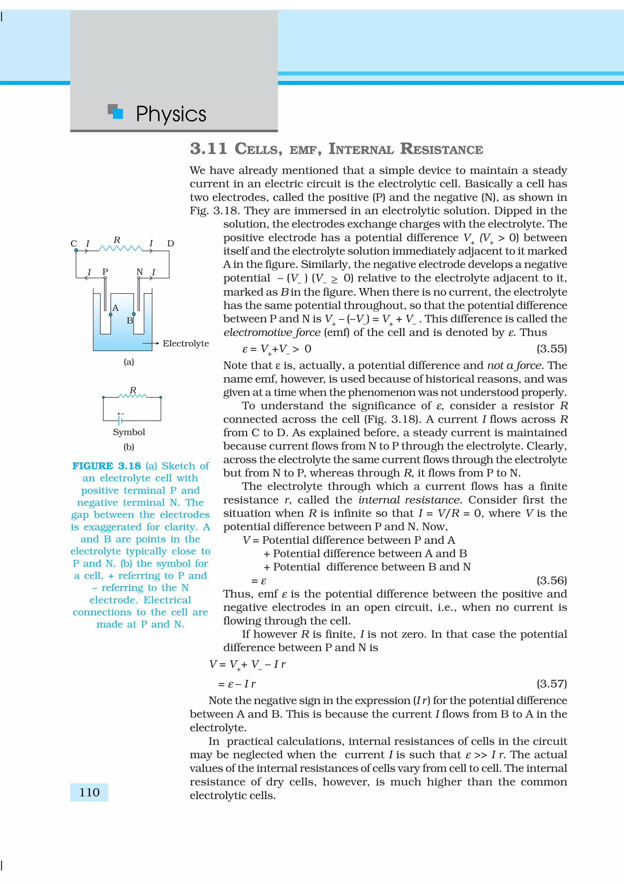
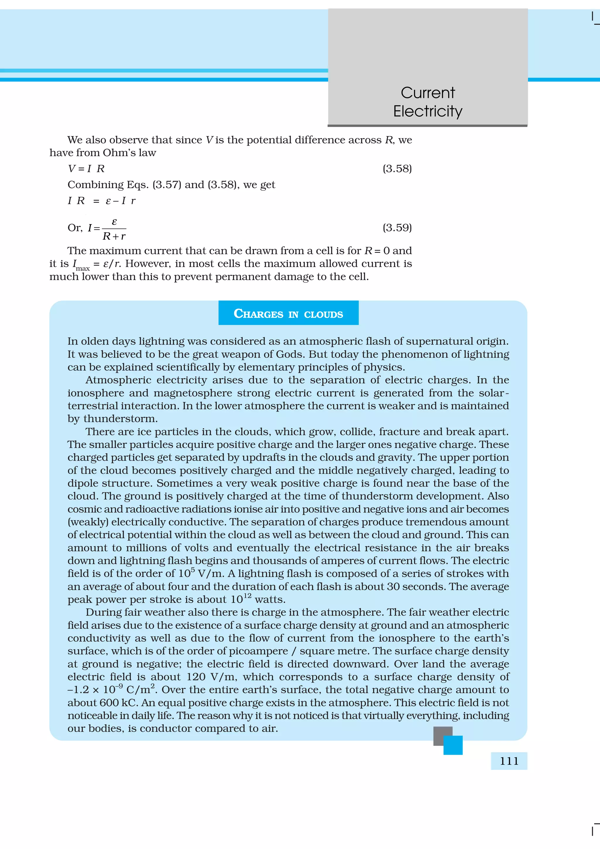
116. Physics
112
EXAMPLE3.5
Example 3.5 A network of resistors is connected to a 16 V battery
with internal resistance of 1Ω, as shown in Fig. 3.19: (a) Compute
the equivalent resistance of the network. (b) Obtain the current in
each resistor. (c) Obtain the voltage drops VAB
, VBC
and VCD
.
FIGURE 3.19
Solution
(a) The network is a simple series and parallel combination of
resistors. First the two 4Ω resistors in parallel are equivalent to a
resistor = [(4 × 4)/(4 + 4)] Ω = 2 Ω.
In the same way, the 12 Ω and 6 Ω resistors in parallel are
equivalent to a resistor of
[(12 × 6)/(12 + 6)] Ω = 4 Ω.
The equivalent resistance R of the network is obtained by
combining these resistors (2 Ω and 4 Ω) with 1 Ω in series,
that is,
R = 2 Ω + 4 Ω + 1 Ω = 7 Ω.
(b) The total current I in the circuit is
16
2 A
(7 1)
V
I
R r
ε
= = =
+ + Ω
Consider the resistors between A and B. If I1
is the current in one
of the 4 Ω resistors and I2
the current in the other,
I1
× 4 = I2
× 4
that is, I1
= I2
, which is otherwise obvious from the symmetry of
the two arms. But I1
+ I2
= I = 2 A. Thus,
I1
= I2
= 1 A
that is, current in each 4 Ω resistor is 1 A. Current in 1 Ω resistor
between B and C would be 2 A.
Now, consider the resistances between C and D. If I3
is the current
in the 12 Ω resistor, and I4
in the 6 Ω resistor,
I3
× 12 = I4
× 6, i.e., I4
= 2I3
But, I3
+ I4
= I = 2 A
Thus, I3
=
2
3
 
   A, I4
=
4
3
 
   A
that is, the current in the 12 Ω resistor is (2/3) A, while the current
in the 6 Ω resistor is (4/3) A.
(c) The voltage drop across AB is
VAB
= I1
× 4 = 1 A × 4 Ω = 4 V,
This can also be obtained by multiplying the total current between
A and B by the equivalent resistance between A and B, that is,

117. Current
Electricity
113
EXAMPLE3.5
VAB
= 2 A × 2 Ω = 4 V
The voltage drop across BC is
VBC
= 2 A × 1 Ω = 2 V
Finally, the voltage drop across CD is
VCD
= 12 Ω × I3
= 12 Ω ×
2
3
 
   A = 8 V.
This can alternately be obtained by multiplying total current
between C and D by the equivalent resistance between C and D,
that is,
VCD
= 2 A × 4 Ω = 8 V
Note that the total voltage drop across AD is 4 V + 2 V + 8 V = 14 V.
Thus, the terminal voltage of the battery is 14 V, while its emf is 16 V.
The loss of the voltage (= 2 V) is accounted for by the internal resistance
1 Ω of the battery [2 A × 1 Ω = 2 V].
3.12 CELLS IN SERIES AND IN PARALLEL
Like resistors, cells can be combined together in an electric circuit. And
like resistors, one can, for calculating currents and voltages in a circuit,
replace a combination of cells by an equivalent cell.
FIGURE 3.20 Two cells of emf’s ε1
and ε2
in the series. r1
, r2
are their
internal resistances. For connections across A and C, the combination
can be considered as one cell of emf εeq
and an internal resistance req
.
Consider first two cells in series (Fig. 3.20), where one terminal of the
two cells is joined together leaving the other terminal in either cell free.
ε1
, ε2
are the emf’s of the two cells and r1
, r2
their internal resistances,
respectively.
Let V (A), V (B), V (C) be the potentials at points A, B and C shown in
Fig. 3.20. Then V (A) – V (B) is the potential difference between the positive
and negative terminals of the first cell. We have already calculated it in
Eq. (3.57) and hence,
AB 1 1(A) – (B) –V V V I rε≡ = (3.60)
Similarly,
BC 2 2(B)– (C) –V V V I rε≡ = (3.61)
Hence, the potential difference between the terminals A and C of the
combination is
( ) ( ) ( ) ( )AC (A) – (C) A – B B – CV V V V V V V≡ = +      
( ) ( )1 2 1 2– I r rε ε= + + (3.62)

118. Physics
114
If we wish to replace the combination by a single cell between A and
C of emf εeq
and internal resistance req
, we would have
VAC
= εeq
– I req
(3.63)
Comparing the last two equations, we get
εeq
= ε1
+ ε2
(3.64)
and req
= r1
+ r2
(3.65)
In Fig.3.20, we had connected the negative electrode of the first to the
positive electrode of the second. If instead we connect the two negatives,
Eq. (3.61) would change to VBC = –ε2–Ir2 and we will get
εeq = ε1 – ε2 (ε1 > ε2) (3.66)
The rule for series combination clearly can be extended to any number
of cells:
(i) The equivalent emf of a series combination of n cells is just the sum of
their individual emf’s, and
(ii) The equivalent internal resistance of a series combination of n cells is
just the sum of their internal resistances.
This is so, when the current leaves each cell from the positive
electrode. If in the combination, the current leaves any cell from
the negative electrode, the emf of the cell enters the expression
for εeq
with a negative sign, as in Eq. (3.66).
Next, consider a parallel combination of the cells (Fig. 3.21).
I1
and I2
are the currents leaving the positive electrodes of the
cells. At the point B1
, I1
and I2
flow in whereas the current I flows
out. Since as much charge flows in as out, we have
I = I1 + I2 (3.67)
Let V (B1
) and V (B2
) be the potentials at B1
and B2
, respectively.
Then, considering the first cell, the potential difference across its
terminals is V (B1
) – V (B2
). Hence, from Eq. (3.57)
( ) ( )1 2 1 1 1– –V V B V B I rε≡ = (3.68)
Points B1
and B2
are connected exactly similarly to the second
cell. Hence considering the second cell, we also have
( ) ( )1 2 2 2 2– –V V B V B I rε≡ = (3.69)
Combining the last three equations
1 2I I I= +
1 2 1 2
1 2 1 2 1 2
– – 1 1
–
V V
V
r r r r r r
ε ε ε ε   
= + = + +      
(3.70)
Hence, V is given by,
1 2 2 1 1 2
1 2 1 2
–
r r r r
V I
r r r r
ε ε+
=
+ +
(3.71)
If we want to replace the combination by a single cell, between B1 and
B2
, of emf εeq
and internal resistance req
, we would have
V = εeq
– I req
(3.72)
FIGURE 3.21 Two cells in
parallel. For connections
across A and C, the
combination can be
replaced by one cell of emf
εeq
and internal resistances
req
whose values are given in
Eqs. (3.64) and (3.65).

119. Current
Electricity
115
The last two equations should be the same and hence
1 2 2 1
1 2
eq
r r
r r
ε ε
ε
+
=
+
(3.73)
1 2
1 2
eq
r r
r
r r
=
+ (3.74)
We can put these equations in a simpler way,
1 2
1 1 1
eqr r r
= + (3.75)
1 2
1 2
eq
eqr r r
ε ε ε
= + (3.76)
In Fig. (3.21), we had joined the positive terminals
together and similarly the two negative ones, so that the
currents I1, I2 flow out of positive terminals. If the negative
terminal of the second is connected to positive terminal
of the first, Eqs. (3.75) and (3.76) would still be valid with
ε 2 → –ε2
Equations (3.75) and (3.76) can be extended easily.
If there an n cells of emf ε1
, . . . εn
and of internal resistances
r1, . . . rn respectively, connected in parallel, the
combination is equivalent to a single cell of emf εeq
and
internal resistance req
, such that
1
1 1 1
eq nr r r
= + +L (3.77)
1
1
eq n
eq nr r r
ε εε
= + +L (3.78)
3.13 KIRCHHOFF’S RULES
Electric circuits generally consist of a number of resistors and cells
interconnected sometimes in a complicated way. The formulae we have
derived earlier for series and parallel combinations of resistors are not
always sufficient to determine all the currents and potential differences
in the circuit. Two rules, called Kirchhoff’s rules, are very useful for
analysis of electric circuits.
Given a circuit, we start by labelling currents in each resistor by a
symbol, say I, and a directed arrow to indicate that a current I flows
along the resistor in the direction indicated. If ultimately I is determined
to be positive, the actual current in the resistor is in the direction of the
arrow. If I turns out to be negative, the current actually flows in a direction
opposite to the arrow. Similarly, for each source (i.e., cell or some other
source of electrical power) the positive and negative electrodes are labelled
as well as a directed arrow with a symbol for the current flowing through
the cell. This will tell us the potential difference, V = V (P) – V (N) = ε – I r
Gustav Robert Kirchhoff
(1824 – 1887) German
physicist, professor at
Heidelberg and at
Berlin. Mainly known for
his development of
spectroscopy, he also
made many important
contributions to mathe-
matical physics, among
them, his first and
second rules for circuits.
GUSTAVROBERTKIRCHHOFF(1824–1887)

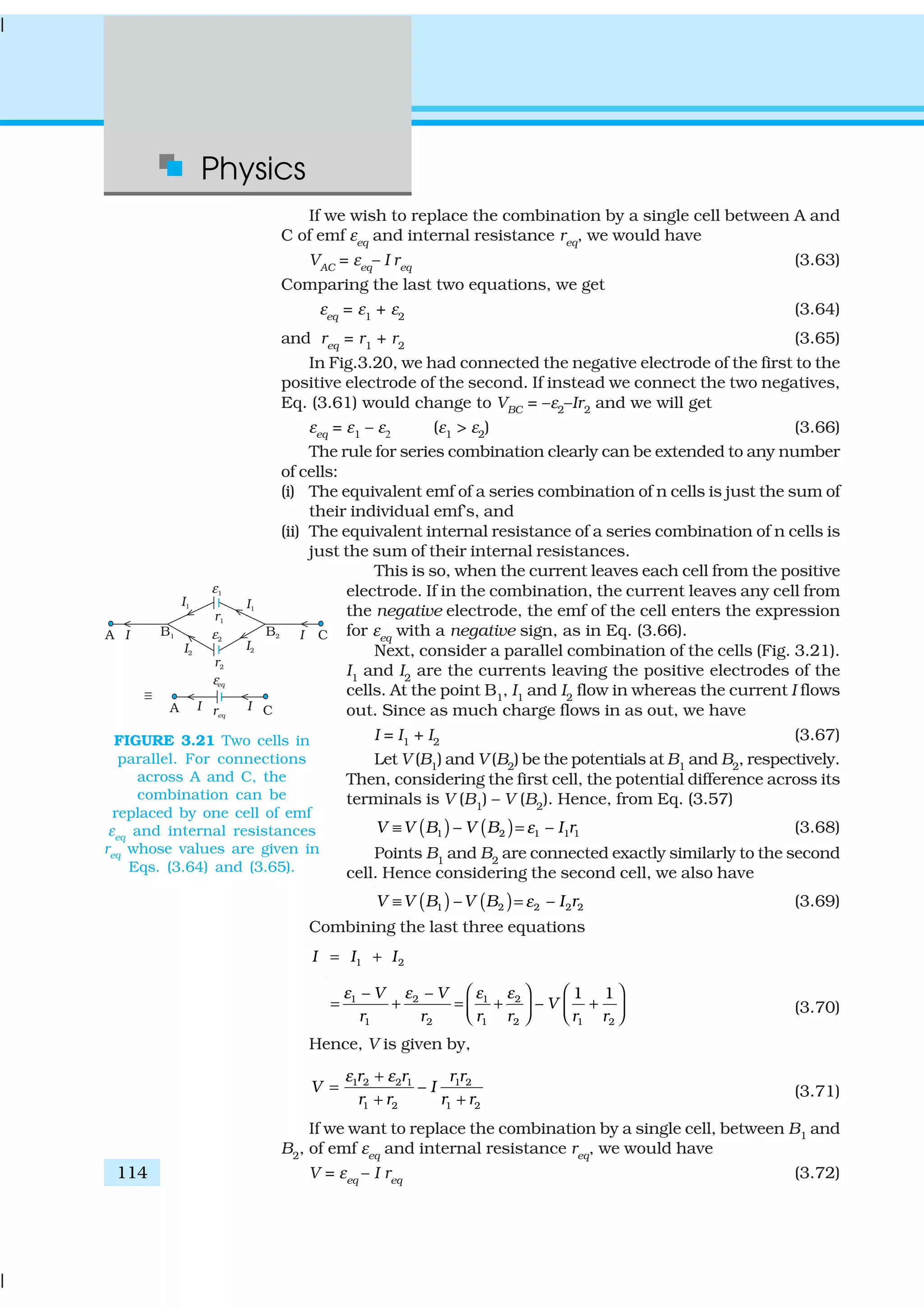
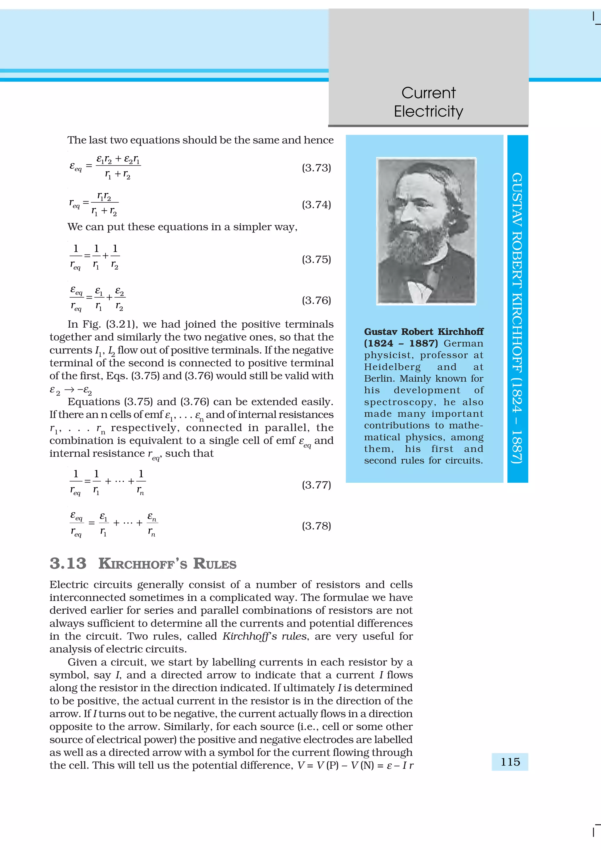
120. Physics
116
EXAMPLE3.6
[Eq. (3.57) between the positive terminal P and the negative terminal N; I
here is the current flowing from N to P through the cell]. If, while labelling
the current I through the cell one goes from P to N,
then of course
V = ε + I r (3.79)
Having clarified labelling, we now state the rules
and the proof:
(a) Junction rule: At any junction, the sum of the
currents entering the junction is equal to the
sum of currents leaving the junction (Fig. 3.22).
This applies equally well if instead of a junction of
several lines, we consider a point in a line.
The proof of this rule follows from the fact that
when currents are steady, there is no accumulation
of charges at any junction or at any point in a line.
Thus, the total current flowing in, (which is the rate
at which charge flows into the junction), must equal
the total current flowing out.
(b) Loop rule: The algebraic sum of changes in
potential around any closed loop involving
resistors and cells in the loop is zero (Fig. 3.22).
This rule is also obvious, since electric potential is
dependent on the location of the point. Thus starting with any point if we
come back to the same point, the total change must be zero. In a closed
loop, we do come back to the starting point and hence the rule.
Example 3.6 A battery of 10 V and negligible internal resistance is
connected across the diagonally opposite corners of a cubical network
consisting of 12 resistors each of resistance 1 Ω (Fig. 3.23). Determine
the equivalent resistance of the network and the current along each
edge of the cube.
FIGURE 3.23
FIGURE 3.22 At junction a the current
leaving is I1
+ I2
and current entering is I3
.
The junction rule says I3
= I1
+ I2
. At point
h current entering is I1
. There is only one
current leaving h and by junction rule
that will also be I1
. For the loops ‘ahdcba’
and ‘ahdefga’, the loop rules give –30I1
–
41 I3
+ 45 = 0 and –30I1
+ 21 I2
– 80 = 0.

121. Current
Electricity
117
EXAMPLE3.6
Solution The network is not reducible to a simple series and parallel
combinations of resistors. There is, however, a clear symmetry in the
problem which we can exploit to obtain the equivalent resistance of
the network.
The paths AA′, AD and AB are obviously symmetrically placed in the
network. Thus, the current in each must be the same, say, I. Further,
at the corners A′, B and D, the incoming current I must split equally
into the two outgoing branches. In this manner, the current in all
the 12 edges of the cube are easily written down in terms of I, using
Kirchhoff’s first rule and the symmetry in the problem.
Next take a closed loop, say, ABCC′EA, and apply Kirchhoff’s second
rule:
–IR – (1/2)IR – IR + ε = 0
where R is the resistance of each edge and ε the emf of battery. Thus,
ε =
5
2
I R
The equivalent resistance Req
of the network is
5
3 6
eqR R
I
ε
= =
For R = 1 Ω, Req
= (5/6) Ω and for ε = 10 V, the total current (= 3I) in
the network is
3I = 10 V/(5/6) Ω = 12 A, i.e., I = 4 A
The current flowing in each edge can now be read off from the
Fig. 3.23.
It should be noted that because of the symmetry of the network, the
great power of Kirchhoff’s rules has not been very apparent in Example 3.6.
In a general network, there will be no such simplification due to
symmetry, and only by application of Kirchhoff’s rules to junctions and
closed loops (as many as necessary to solve the unknowns in the network)
can we handle the problem. This will be illustrated in Example 3.7.
Example 3.7 Determine the current in each branch of the network
shown in Fig. 3.24.
FIGURE 3.24
SimilationforapplicationofKirchhoffísrules:
http://www.phys.hawaii.edu/~teb/optics/java/kirch3/
EXAMPLE3.7

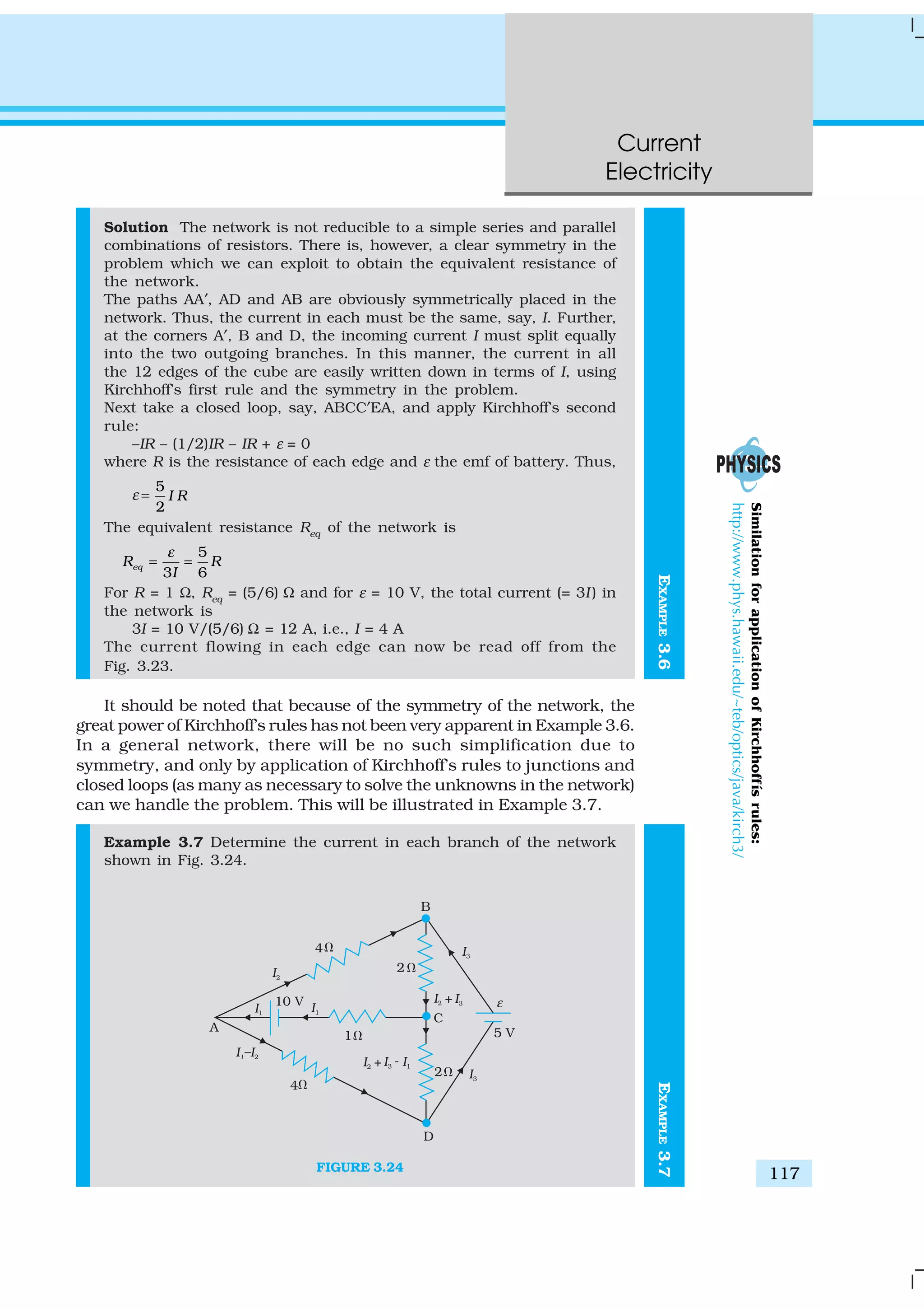
122. Physics
118
EXAMPLE3.7
Solution Each branch of the network is assigned an unknown current
to be determined by the application of Kirchhoff’s rules. To reduce
the number of unknowns at the outset, the first rule of Kirchhoff is
used at every junction to assign the unknown current in each branch.
We then have three unknowns I1
, I2
and I3
which can be found by
applying the second rule of Kirchhoff to three different closed loops.
Kirchhoff’s second rule for the closed loop ADCA gives,
10 – 4(I1
– I2
) + 2(I2
+ I3
– I1
) – I1
= 0 [3.80(a)]
that is, 7I1
– 6I2
– 2I3
= 10
For the closed loop ABCA, we get
10 – 4I2
– 2 (I2
+ I3
) – I1
= 0
that is, I1
+ 6I2
+ 2I3
=10 [3.80(b)]
For the closed loop BCDEB, we get
5 – 2 (I2
+ I3
) – 2 (I2
+ I3
– I1
) = 0
that is, 2I1
– 4I2
– 4I3
= –5 [3.80(c)]
Equations (3.80 a, b, c) are three simultaneous equations in three
unknowns. These can be solved by the usual method to give
I1
= 2.5A, I2
=
5
8
A, I3
=
7
1
8
A
The currents in the various branches of the network are
AB :
5
8
A, CA :
1
2
2
A, DEB :
7
1
8
A
AD :
7
1
8
A, CD : 0 A, BC :
1
2
2
A
It is easily verified that Kirchhoff’s second rule applied to the
remaining closed loops does not provide any additional independent
equation, that is, the above values of currents satisfy the second
rule for every closed loop of the network. For example, the total voltage
drop over the closed loop BADEB
5 15
5 V 4 V 4 V
8 8
   
+ × − ×      
equal to zero, as required by Kirchhoff’s second rule.
3.14 WHEATSTONE BRIDGE
As an application of Kirchhoff’s rules consider the circuit shown in
Fig. 3.25, which is called the Wheatstone bridge. The bridge has
four resistors R1, R2, R3 and R4. Across one pair of diagonally opposite
points (A and C in the figure) a source is connected. This (i.e., AC) is
called the battery arm. Between the other two vertices, B and D, a
galvanometer G (which is a device to detect currents) is connected. This
line, shown as BD in the figure, is called the galvanometer arm.
For simplicity, we assume that the cell has no internal resistance. In
general there will be currents flowing across all the resistors as well as a
current Ig through G. Of special interest, is the case of a balanced bridge
where the resistors are such that Ig
= 0. We can easily get the balance
condition, such that there is no current through G. In this case, the
Kirchhoff’s junction rule applied to junctions D and B (see the figure)

123. Current
Electricity
119
immediately gives us the relations I1
= I3
and I2
= I4
. Next, we apply
Kirchhoff’s loop rule to closed loops ADBA and CBDC. The first
loop gives
–I1 R1 + 0 + I2 R2 = 0 (Ig = 0) (3.81)
and the second loop gives, upon using I3
= I1
, I4
= I2
I2
R4
+ 0 – I1
R3
= 0 (3.82)
From Eq. (3.81), we obtain,
1 2
2 1
I R
I R
=
whereas from Eq. (3.82), we obtain,
1 4
2 3
I R
I R
=
Hence, we obtain the condition
2 4
1 3
R R
R R
= [3.83(a)]
This last equation relating the four resistors is called the balance
condition for the galvanometer to give zero or null deflection.
The Wheatstone bridge and its balance condition provide a practical
method for determination of an unknown resistance. Let us suppose we
have an unknown resistance, which we insert in the fourth arm; R4
is
thus not known. Keeping known resistances R1
and R2
in the first and
second arm of the bridge, we go on varying R3
till the galvanometer shows
a null deflection. The bridge then is balanced, and from the balance
condition the value of the unknown resistance R4
is given by,
2
4 3
1
R
R R
R
= [3.83(b)]
A practical device using this principle is called the meter bridge. It
will be discussed in the next section.
Example 3.8 The four arms of a Wheatstone bridge (Fig. 3.26) have
the following resistances:
AB = 100Ω, BC = 10Ω, CD = 5Ω, and DA = 60Ω.
FIGURE 3.26
FIGURE 3.25
EXAMPLE3.8

124. Physics
120
EXAMPLE3.8
A galvanometer of 15Ω resistance is connected across BD. Calculate
the current through the galvanometer when a potential difference of
10 V is maintained across AC.
Solution Considering the mesh BADB, we have
100I1
+ 15Ig
– 60I2
= 0
or 20I1
+ 3Ig
– 12I2
= 0 [3.84(a)]
Considering the mesh BCDB, we have
10 (I1
– Ig
) – 15Ig
– 5 (I2
+ Ig
) = 0
10I1
– 30Ig
–5I2
= 0
2I1
– 6Ig
– I2
= 0 [3.84(b)]
Considering the mesh ADCEA,
60I2
+ 5 (I2
+ Ig
) = 10
65I2
+ 5Ig
= 10
13I2
+ Ig
= 2 [3.84(c)]
Multiplying Eq. (3.84b) by 10
20I1
– 60Ig
– 10I2
= 0 [3.84(d)]
From Eqs. (3.84d) and (3.84a) we have
63Ig
– 2I2
= 0
I2
= 31.5Ig
[3.84(e)]
Substituting the value of I2
into Eq. [3.84(c)], we get
13 (31.5Ig
) + Ig
= 2
410.5 Ig
= 2
Ig
= 4.87 mA.
3.15 METER BRIDGE
The meter bridge is shown in Fig. 3.27. It consists of
a wire of length 1m and of uniform cross sectional
area stretched taut and clamped between two thick
metallic strips bent at right angles, as shown. The
metallic strip has two gaps across which resistors can
be connected. The end points where the wire is
clamped are connected to a cell through a key. One
end of a galvanometer is connected to the metallic
strip midway between the two gaps. The other end of
the galvanometer is connected to a ‘jockey’. The jockey
is essentially a metallic rod whose one end has a
knife-edge which can slide over the wire to make
electrical connection.
R is an unknown resistance whose value we want to determine. It is
connected across one of the gaps. Across the other gap, we connect a
FIGURE 3.27 A meter bridge. Wire AC
is 1 m long. R is a resistance to be
measured and S is a standard
resistance.

125. Current
Electricity
121
standard known resistance S. The jockey is connected to some point D
on the wire, a distance l cm from the end A. The jockey can be moved
along the wire. The portion AD of the wire has a resistance Rcml, where
Rcm
is the resistance of the wire per unit centimetre. The portion DC of
the wire similarly has a resistance Rcm
(100-l).
The four arms AB, BC, DA and CD [with resistances R, S, Rcm l and
Rcm
(100-l)] obviously form a Wheatstone bridge with AC as the battery
arm and BD the galvanometer arm. If the jockey is moved along the wire,
then there will be one position where the galvanometer will show no
current. Let the distance of the jockey from the end A at the balance
point be l= l1
. The four resistances of the bridge at the balance point then
are R, S, Rcm l1 and Rcm(100–l1). The balance condition, Eq. [3.83(a)]
gives
( )
1 1
1 1100 – 100 –
cm
cm
R l lR
S R l l
= = (3.85)
Thus, once we have found out l1
, the unknown resistance R is known
in terms of the standard known resistance S by
1
1100 –
l
R S
l
= (3.86)
By choosing various values of S, we would get various values of l1
,
and calculate R each time. An error in measurement of l1 would naturally
result in an error in R. It can be shown that the percentage error in R can
be minimised by adjusting the balance point near the middle of the
bridge, i.e., when l1 is close to 50 cm. (This requires a suitable choice
of S.)
Example 3.9 In a metre bridge (Fig. 3.27), the null point is found at a
distance of 33.7 cm from A. If now a resistance of 12Ω is connected in
parallel with S, the null point occurs at 51.9 cm. Determine the values
of R and S.
Solution From the first balance point, we get
33.7
66.3
R
S
= (3.87)
After S is connected in parallel with a resistance of 12Ω , the resistance
across the gap changes from S to Seq
, where
12
12
eq
S
S
S
=
+
and hence the new balance condition now gives
( )1251.9
48.1 12eq
R SR
S S
+
= = (3.88)
Substituting the value of R/S from Eq. (3.87), we get
51.9 12 33.7
48.1 12 66.3
S +
= g
which gives S = 13.5Ω. Using the value of R/S above, we get
R = 6.86 Ω.
EXAMPLE3.9

126. Physics
122
3.16 POTENTIOMETER
This is a versatile instrument. It is basically a long piece of uniform wire,
sometimes a few meters in length across which a standard cell is
connected. In actual design, the wire is sometimes cut in several pieces
placed side by side and connected at the ends by thick metal strip.
(Fig. 3.28). In the figure, the wires run from A to C. The small vertical
portions are the thick metal strips connecting the various sections of
the wire.
A current I flows through the wire which can be varied by a variable
resistance (rheostat, R) in the circuit. Since the wire is uniform, the
potential difference between A and any point at a distance l from A is
( )ε φ=l l (3.89)
where φ is the potential drop per unit length.
Figure 3.28 (a) shows an application of the potentiometer to compare
the emf of two cells of emf ε1
and ε2
. The points marked 1, 2, 3 form a two
way key. Consider first a position of the key where 1 and 3 are connected
so that the galvanometer is connected to ε1
. The jockey
is moved along the wire till at a point N1
, at a distance l1
from A, there is no deflection in the galvanometer. We
can apply Kirchhoff’s loop rule to the closed loop
AN1
G31A and get,
φ l1 + 0 – ε1 = 0 (3.90)
Similarly, if another emf ε2
is balanced against l2
(AN2
)
φ l2
+ 0 – ε2
= 0 (3.91)
From the last two equations
1 1
2 2
l
l
ε
ε
= (3.92)
This simple mechanism thus allows one to compare
the emf’s of any two sources. In practice one of the cells
is chosen as a standard cell whose emf is known to a
high degree of accuracy. The emf of the other cell is then
easily calculated from Eq. (3.92).
We can also use a potentiometer to measure internal
resistance of a cell [Fig. 3.28 (b)]. For this the cell (emf ε )
whose internal resistance (r) is to be determined is
connected across a resistance box through a key K2
, as
shown in the figure. With key K2
open, balance is
obtained at length l1 (AN1). Then,
ε = φ l1
[3.93(a)]
When key K2
is closed, the cell sends a current (I )
through the resistance box (R). If V is the terminal
potential difference of the cell and balance is obtained at
length l2
(AN2
),
V = φ l2
[3.93(b)]
FIGURE 3.28 A potentiometer. G is
a galvanometer and R a variable
resistance (rheostat). 1, 2, 3 are
terminals of a two way key
(a) circuit for comparing emfs of two
cells; (b) circuit for determining
internal resistance of a cell.

127. Current
Electricity
123
So, we have ε/V = l1
/l2
[3.94(a)]
But, ε = I (r + R) and V = IR. This gives
ε/V = (r+R)/R [3.94(b)]
From Eq. [3.94(a)] and [3.94(b)] we have
(R+r)/R = l1
/l2
1
2
– 1
l
r R
l
 
=   
(3.95)
Using Eq. (3.95) we can find the internal resistance of a given cell.
The potentiometer has the advantage that it draws no current from
the voltage source being measured. As such it is unaffected by the internal
resistance of the source.
Example 3.10 A resistance of R Ω draws current from a
potentiometer. The potentiometer has a total resistance R0
Ω
(Fig. 3.29). A voltage V is supplied to the potentiometer. Derive an
expression for the voltage across R when the sliding contact is in the
middle of the potentiometer.
FIGURE 3.29
Solution While the slide is in the middle of the potentiometer only
half of its resistance (R0
/2) will be between the points A and B. Hence,
the total resistance between A and B, say, R1
, will be given by the
following expression:
1 0
1 1 1
( /2)R R R
= +
0
1
0 2
R R
R
R R
=
+
The total resistance between A and C will be sum of resistance between
A and B and B and C, i.e., R1
+ R0
/2
∴ The current flowing through the potentiometer will be
1 0 1 0
2
/2 2
V V
I
R R R R
= =
+ +
The voltage V1
taken from the potentiometer will be the product of
current I and resistance R1
,
V1
= I R1
= 1
1 0
2
2
V
R
R R
 
× + 
EXAMPLE3.10

128. Physics
124
EXAMPLE3.10
Substituting for R1
, we have a
0
1
00
0
0
2
2
2
2
R RV
V
R RR R
R
R R
×
= ×
+ ×
+ + 
1
0
2
2 2
VR
V
R R R
=
+ +
or V1
0
2
4
VR
R R
=
+
.
SUMMARY
1. Current through a given area of a conductor is the net charge passing
per unit time through the area.
2. To maintain a steady current, we must have a closed circuit in which
an external agency moves electric charge from lower to higher potential
energy. The work done per unit charge by the source in taking the
charge from lower to higher potential energy (i.e., from one terminal
of the source to the other) is called the electromotive force, or emf, of
the source. Note that the emf is not a force; it is the voltage difference
between the two terminals of a source in open circuit.
3. Ohm’s law: The electric current I flowing through a substance is
proportional to the voltage V across its ends, i.e., V ∝ I or V = RI,
where R is called the resistance of the substance. The unit of resistance
is ohm: 1Ω = 1 V A–1
.
4. The resistance R of a conductor depends on its length l and constant
cross-sectional area A through the relation,
l
R
A
ρ
=
where ρ, called resistivity is a property of the material and depends on
temperature and pressure.
5. Electrical resistivity of substances varies over a very wide range. Metals
have low resistivity, in the range of 10–8
Ω m to 10–6
Ω m. Insulators
like glass and rubber have 1022
to 1024
times greater resistivity.
Semiconductors like Si and Ge lie roughly in the middle range of
resistivity on a logarithmic scale.
6. In most substances, the carriers of current are electrons; in some
cases, for example, ionic crystals and electrolytic liquids, positive and
negative ions carry the electric current.
7. Current density j gives the amount of charge flowing per second per
unit area normal to the flow,
j = nq vd
where n is the number density (number per unit volume) of charge
carriers each of charge q, and vd is the drift velocity of the charge
carriers. For electrons q = – e. If j is normal to a cross-sectional area
A and is constant over the area, the magnitude of the current I through
the area is nevd
A.

129. Current
Electricity
125
8. Using E = V/l, I = nevd
A, and Ohm’s law, one obtains
2
d
eE ne
v
m m
ρ=
The proportionality between the force eE on the electrons in a metal
due to the external field E and the drift velocity vd (not acceleration)
can be understood, if we assume that the electrons suffer collisions
with ions in the metal, which deflect them randomly. If such collisions
occur on an average at a time interval τ,
vd
= aτ = eEτ/m
where a is the acceleration of the electron. This gives
2
m
ne
ρ
τ
=
9. In the temperature range in which resistivity increases linearly with
temperature, the temperature coefficient of resistivity α is defined as
the fractional increase in resistivity per unit increase in temperature.
10. Ohm’s law is obeyed by many substances, but it is not a fundamental
law of nature. It fails if
(a) V depends on I non-linearly.
(b) the relation between V and I depends on the sign of V for the same
absolute value of V.
(c) The relation between V and I is non-unique.
An example of (a) is when ρ increases with I (even if temperature is
kept fixed). A rectifier combines features (a) and (b). GaAs shows the
feature (c).
11. When a source of emf ε is connected to an external resistance R, the
voltage Vext
across R is given by
Vext = IR = R
R r
ε
+
where r is the internal resistance of the source.
12. (a) Total resistance R of n resistors connected in series is given by
R = R1
+ R2
+..... + Rn
(b) Total resistance R of n resistors connected in parallel is given by
1 2
1 1 1 1
......
n
R R R R
= + + +
13. Kirchhoff’s Rules –
(a) Junction Rule: At any junction of circuit elements, the sum of
currents entering the junction must equal the sum of currents
leaving it.
(b) Loop Rule: The algebraic sum of changes in potential around any
closed loop must be zero.
14. The Wheatstone bridge is an arrangement of four resistances – R1
, R2
,
R3
, R4
as shown in the text. The null-point condition is given by
31
2 4
RR
R R
=
using which the value of one resistance can be determined, knowing
the other three resistances.
15. The potentiometer is a device to compare potential differences. Since
the method involves a condition of no current flow, the device can be
used to measure potential difference; internal resistance of a cell and
compare emf’s of two sources.

130. Physics
126
POINTS TO PONDER
1. Current is a scalar although we represent current with an arrow.
Currents do not obey the law of vector addition. That current is a
scalar also follows from it’s definition. The current I through an area
of cross-section is given by the scalar product of two vectors:
I = j . ∆S
where j and ∆S are vectors.
2. Refer to V-I curves of a resistor and a diode as drawn in the text. A
resistor obeys Ohm’s law while a diode does not. The assertion that
V = IR is a statement of Ohm’s law is not true. This equation defines
resistance and it may be applied to all conducting devices whether
they obey Ohm’s law or not. The Ohm’s law asserts that the plot of I
versus V is linear i.e., R is independent of V.
Equation E = ρ j leads to another statement of Ohm’s law, i.e., a
conducting material obeys Ohm’s law when the resistivity of the
material does not depend on the magnitude and direction of applied
electric field.
3. Homogeneous conductors like silver or semiconductors like pure
germanium or germanium containing impurities obey Ohm’s law
within some range of electric field values. If the field becomes too
strong, there are departures from Ohm’s law in all cases.
4. Motion of conduction electrons in electric field E is the sum of (i)
motion due to random collisions and (ii) that due to E. The motion
Physical Quantity Symbol Dimensions Unit Remark
Electric current I [A] A SI base unit
Charge Q, q [T A] C
Voltage, Electric V [M L
2
T
–3
A
–1
] V Work/charge
potential difference
Electromotive force ε [M L
2
T
–3
A
–1
] V Work/charge
Resistance R [M L
2
T
–3
A
–2
] Ω R = V/I
Resistivity ρ [M L
3
T
–3
A
–2
] Ω m R = ρl/A
Electrical σ [M
–1
L
–3
T
3
A
2
] S σ = 1/ρ
conductivity
Electric field E [M L T
–3
A
–1
] V m
–1 Electric force
charge
Drift speed vd
[L T–1
] m s–1
vd
e E
m
=
τ
Relaxation time τ [T] s
Current density j [L
–2
A] A m
–2
current/area
Mobility µ [M L
3
T
–4
A
–1
] m
2
V
–1
s
–1
/dv E

131. Current
Electricity
127
EXERCISES
3.1 The storage battery of a car has an emf of 12 V. If the internal
resistance of the battery is 0.4 Ω, what is the maximum current
that can be drawn from the battery?
3.2 A battery of emf 10 V and internal resistance 3 Ω is connected to a
resistor. If the current in the circuit is 0.5 A, what is the resistance
of the resistor? What is the terminal voltage of the battery when the
circuit is closed?
3.3 (a) Three resistors 1 Ω, 2 Ω, and 3 Ω are combined in series. What
is the total resistance of the combination?
(b) If the combination is connected to a battery of emf 12 V and
negligible internal resistance, obtain the potential drop across
each resistor.
3.4 (a) Three resistors 2 Ω, 4 Ω and 5 Ω are combined in parallel. What
is the total resistance of the combination?
(b) If the combination is connected to a battery of emf 20 V and
negligible internal resistance, determine the current through
each resistor, and the total current drawn from the battery.
3.5 At room temperature (27.0 °C) the resistance of a heating element
is 100 Ω. What is the temperature of the element if the resistance is
found to be 117 Ω, given that the temperature coefficient of the
material of the resistor is 1.70 × 10–4
°C–1
.
3.6 A negligibly small current is passed through a wire of length 15 m
and uniform cross-section 6.0 × 10–7
m2
, and its resistance is
measured to be 5.0 Ω. What is the resistivity of the material at the
temperature of the experiment?
3.7 A silver wire has a resistance of 2.1 Ω at 27.5 °C, and a resistance
of 2.7 Ω at 100 °C. Determine the temperature coefficient of
resistivity of silver.
3.8 A heating element using nichrome connected to a 230 V supply
draws an initial current of 3.2 A which settles after a few seconds to
due to random collisions averages to zero and does not contribute to
vd
(Chapter 11, Textbook of Class XI). vd
, thus is only due to applied
electric field on the electron.
5. The relation j = ρ v should be applied to each type of charge carriers
separately. In a conducting wire, the total current and charge density
arises from both positive and negative charges:
j = ρ+
v+
+ ρ–
v–
ρ = ρ+
+ ρ–
Now in a neutral wire carrying electric current,
ρ+
= – ρ–
Further, v+
~ 0 which gives
ρ = 0
j = ρ–
v
Thus, the relation j = ρ v does not apply to the total current charge
density.
6. Kirchhoff’s junction rule is based on conservation of charge and the
outgoing currents add up and are equal to incoming current at a
junction. Bending or reorienting the wire does not change the validity
of Kirchhoff’s junction rule.

132. Physics
128
a steady value of 2.8 A. What is the steady temperature of the heating
element if the room temperature is 27.0 °C? Temperature coefficient
of resistance of nichrome averaged over the temperature range
involved is 1.70 × 10–4
°C–1
.
3.9 Determine the current in each branch of the network shown in
Fig. 3.30:
FIGURE 3.30
3.10 (a) In a metre bridge [Fig. 3.27], the balance point is found to be at
39.5 cm from the end A, when the resistor Y is of 12.5 Ω.
Determine the resistance of X. Why are the connections between
resistors in a Wheatstone or meter bridge made of thick copper
strips?
(b) Determine the balance point of the bridge above if X and Y are
interchanged.
(c) What happens if the galvanometer and cell are interchanged at
the balance point of the bridge? Would the galvanometer show
any current?
3.11 A storage battery of emf 8.0 V and internal resistance 0.5 Ω is being
charged by a 120 V dc supply using a series resistor of 15.5 Ω. What
is the terminal voltage of the battery during charging? What is the
purpose of having a series resistor in the charging circuit?
3.12 In a potentiometer arrangement, a cell of emf 1.25 V gives a balance
point at 35.0 cm length of the wire. If the cell is replaced by another
cell and the balance point shifts to 63.0 cm, what is the emf of the
second cell?
3. 13 The number density of free electrons in a copper conductor
estimated in Example 3.1 is 8.5 × 1028
m–3
. How long does an electron
take to drift from one end of a wire 3.0 m long to its other end? The
area of cross-section of the wire is 2.0 × 10–6
m2
and it is carrying a
current of 3.0 A.
ADDITIONAL EXERCISES
3. 14 The earth’s surface has a negative surface charge density of 10–9
C
m–2
. The potential difference of 400 kV between the top of the
atmosphere and the surface results (due to the low conductivity of
the lower atmosphere) in a current of only 1800 A over the entire
globe. If there were no mechanism of sustaining atmospheric electric

133. Current
Electricity
129
field, how much time (roughly) would be required to neutralise the
earth’s surface? (This never happens in practice because there is a
mechanism to replenish electric charges, namely the continual
thunderstorms and lightning in different parts of the globe). (Radius
of earth = 6.37 × 106
m.)
3.15 (a) Six lead-acid type of secondary cells each of emf 2.0 V and internal
resistance 0.015 Ω are joined in series to provide a supply to a
resistance of 8.5 Ω. What are the current drawn from the supply
and its terminal voltage?
(b) A secondary cell after long use has an emf of 1.9 V and a large
internal resistance of 380 Ω. What maximum current can be drawn
from the cell? Could the cell drive the starting motor of a car?
3.16 Two wires of equal length, one of aluminium and the other of copper
have the same resistance. Which of the two wires is lighter? Hence
explain why aluminium wires are preferred for overhead power cables.
(ρAl
= 2.63 × 10–8
Ω m, ρCu
= 1.72 × 10–8
Ω m, Relative density of
Al = 2.7, of Cu = 8.9.)
3.17 What conclusion can you draw from the following observations on a
resistor made of alloy manganin?
Current Voltage Current Voltage
A V A V
0.2 3.94 3.0 59.2
0.4 7.87 4.0 78.8
0.6 11.8 5.0 98.6
0.8 15.7 6.0 118.5
1.0 19.7 7.0 138.2
2.0 39.4 8.0 158.0
3.18 Answer the following questions:
(a) A steady current flows in a metallic conductor of non-uniform
cross-section. Which of these quantities is constant along the
conductor: current, current density, electric field, drift speed?
(b) Is Ohm’s law universally applicable for all conducting elements?
If not, give examples of elements which do not obey Ohm’s law.
(c) A low voltage supply from which one needs high currents must
have very low internal resistance. Why?
(d) A high tension (HT) supply of, say, 6 kV must have a very large
internal resistance. Why?
3.19 Choose the correct alternative:
(a) Alloys of metals usually have (greater/less) resistivity than that
of their constituent metals.
(b) Alloys usually have much (lower/higher) temperature
coefficients of resistance than pure metals.
(c) The resistivity of the alloy manganin is nearly independent of/
increases rapidly with increase of temperature.
(d) The resistivity of a typical insulator (e.g., amber) is greater than
that of a metal by a factor of the order of (1022
/103
).
3.20 (a) Given n resistors each of resistance R, how will you combine
them to get the (i) maximum (ii) minimum effective resistance?
What is the ratio of the maximum to minimum resistance?
(b) Given the resistances of 1 Ω, 2 Ω, 3 Ω, how will be combine them
to get an equivalent resistance of (i) (11/3) Ω (ii) (11/5) Ω, (iii) 6
Ω, (iv) (6/11) Ω?
(c) Determine the equivalent resistance of networks shown in
Fig. 3.31.

134. Physics
130
FIGURE 3.31
3.21 Determine the current drawn from a 12V supply with internal
resistance 0.5Ω by the infinite network shown in Fig. 3.32. Each
resistor has 1Ω resistance.
FIGURE 3.32
3.22 Figure 3.33 shows a potentiometer with a cell of 2.0 V and internal
resistance 0.40 Ω maintaining a potential drop across the resistor
wire AB. A standard cell which maintains a constant emf of 1.02 V
(for very moderate currents upto a few mA) gives a balance point at
67.3 cm length of the wire. To ensure very low currents drawn from
the standard cell, a very high resistance of 600 kΩ is put in series
with it, which is shorted close to the balance point. The standard
cell is then replaced by a cell of unknown emf ε and the balance
point found similarly, turns out to be at 82.3 cm length of the wire.
FIGURE 3.33
(a) What is the value ε?
(b) What purpose does the high resistance of 600 kΩ have?

135. Current
Electricity
131
(c) Is the balance point affected by this high resistance?
(d) Is the balance point affected by the internal resistance of the
driver cell?
(e) Would the method work in the above situation if the driver cell
of the potentiometer had an emf of 1.0V instead of 2.0V?
(f ) Would the circuit work well for determining an extremely small
emf, say of the order of a few mV (such as the typical emf of a
thermo-couple)? If not, how will you modify the circuit?
3.23 Figure 3.34 shows a potentiometer circuit for comparison of two
resistances. The balance point with a standard resistor R = 10.0 Ω
is found to be 58.3 cm, while that with the unknown resistance X is
68.5 cm. Determine the value of X. What might you do if you failed
to find a balance point with the given cell of emf ε ?
FIGURE 3.34
3.24 Figure 3.35 shows a 2.0 V potentiometer used for the determination
of internal resistance of a 1.5 V cell. The balance point of the cell in
open circuit is 76.3 cm. When a resistor of 9.5 Ω is used in the external
circuit of the cell, the balance point shifts to 64.8 cm length of the
potentiometer wire. Determine the internal resistance of the cell.
FIGURE 3.35

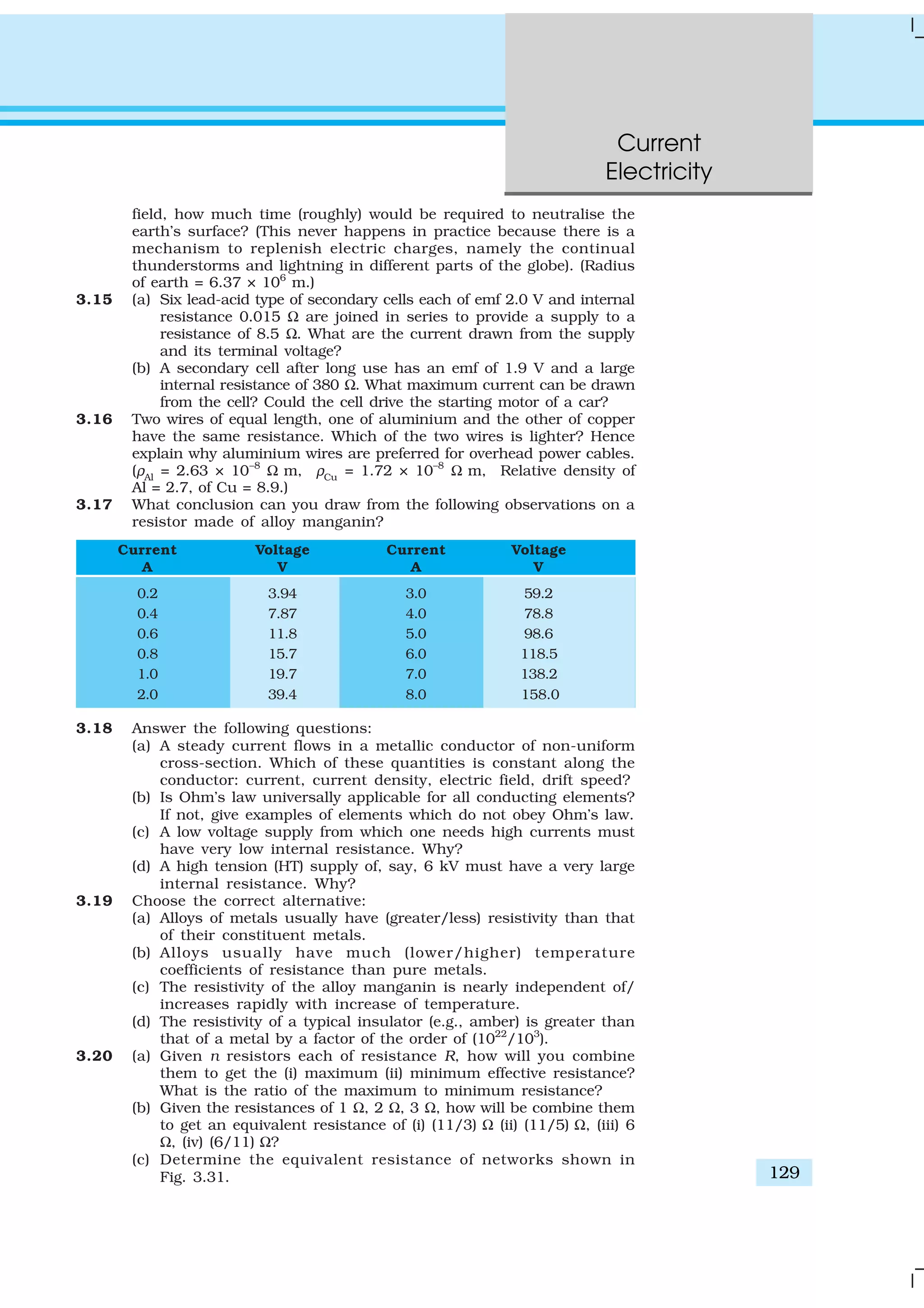
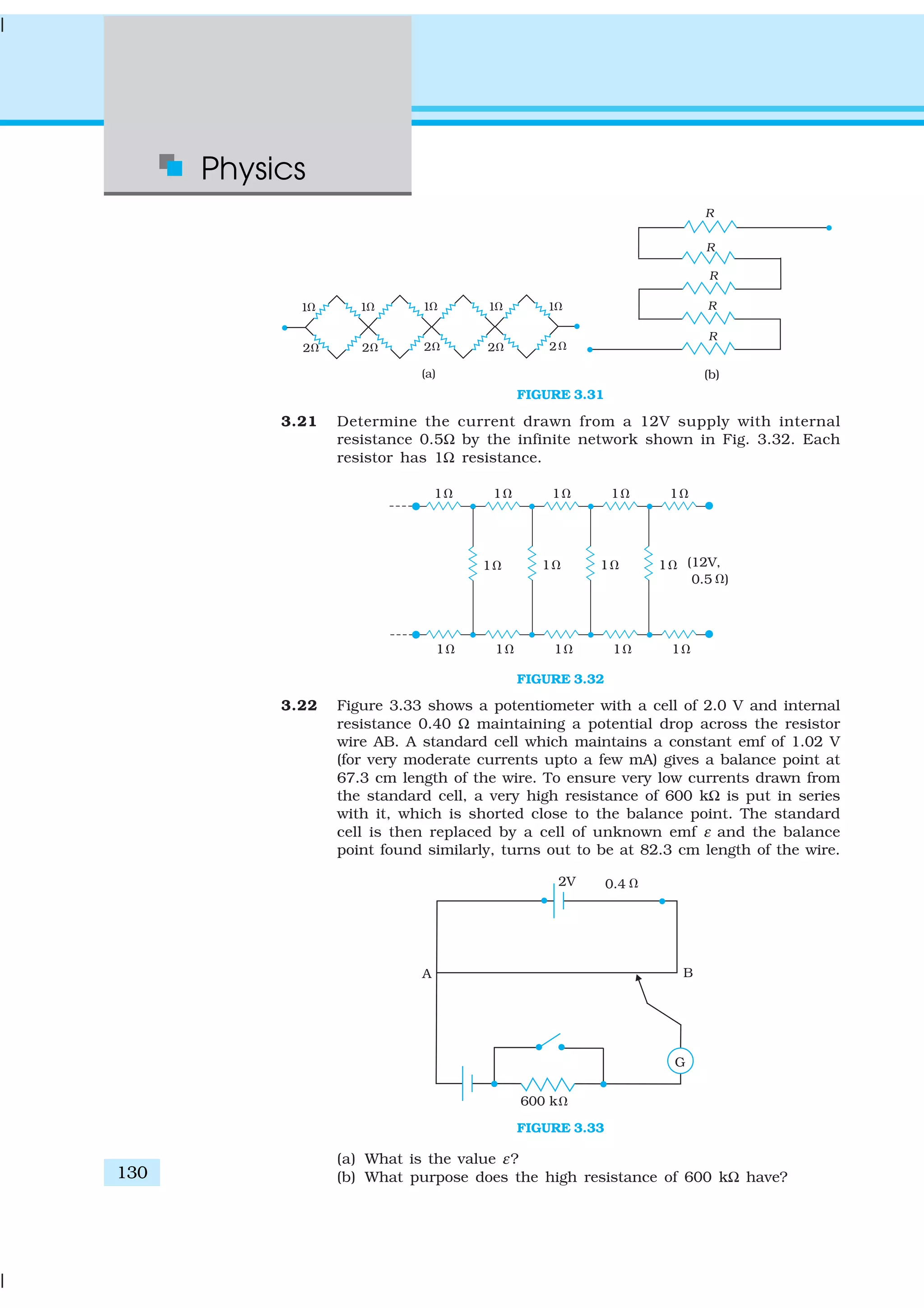
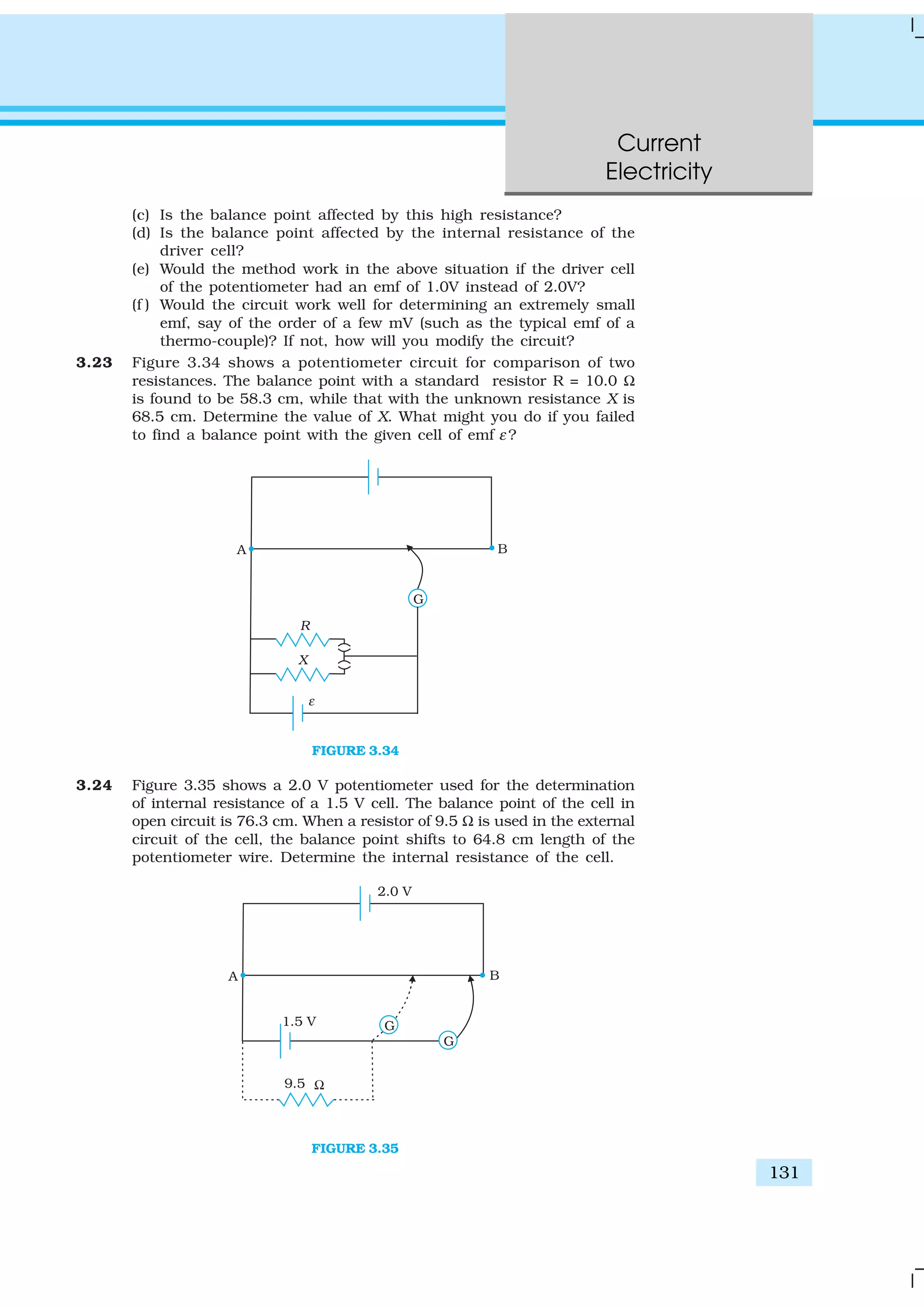
136. 4.1 INTRODUCTION
Both Electricity and Magnetism have been known for more than 2000
years. However, it was only about 200 years ago, in 1820, that it was
realised that they were intimately related*. During a lecture demonstration
in the summer of 1820, the Danish physicist Hans Christian Oersted
noticed that a current in a straight wire caused a noticeable deflection in
a nearby magnetic compass needle. He investigated this phenomenon.
He found that the alignment of the needle is tangential to an imaginary
circle which has the straight wire as its centre and has its plane
perpendicular to the wire. This situation is depicted in Fig.4.1(a). It is
noticeable when the current is large and the needle sufficiently close to
the wire so that the earth’s magnetic field may be ignored. Reversing the
direction of the current reverses the orientation of the needle [Fig. 4.1(b)].
The deflection increases on increasing the current or bringing the needle
closer to the wire. Iron filings sprinkled around the wire arrange
themselves in concentric circles with the wire as the centre [Fig. 4.1(c)].
Oersted concluded that moving charges or currents produced a
magnetic field in the surrounding space.
Following this there was intense experimentation. In 1864, the laws
obeyed by electricity and magnetism were unified and formulated by
Chapter Four
MOVING CHARGES
AND MAGNETISM
* See the box in Chapter 1, Page 3.

137. Moving Charges and
Magnetism
133
James Maxwell who then realised that light was electromagnetic waves.
Radio waves were discovered by Hertz, and produced by J.C.Bose and
G. Marconi by the end of the 19th
century. A remarkable scientific and
technological progress has taken place in the 20th
century. This is due to
our increased understanding of electromagnetism and the invention of
devices for production, amplification, transmission and detection of
electromagnetic waves.
In this chapter, we will see how magnetic field exerts
forces on moving charged particles, like electrons,
protons, and current-carrying wires. We shall also learn
how currents produce magnetic fields. We shall see how
particles can be accelerated to very high energies in a
cyclotron. We shall study how currents and voltages are
detected by a galvanometer.
In this and subsequent Chapter on magnetism,
we adopt the following convention: A current or a
field (electric or magnetic) emerging out of the plane of the
paper is depicted by a dot (¤). A current or a field going
into the plane of the paper is depicted by a cross ( ⊗ )*.
Figures. 4.1(a) and 4.1(b) correspond to these two
situations, respectively.
4.2 MAGNETIC FORCE
4.2.1 Sources and fields
Before we introduce the concept of a magnetic field B, we
shall recapitulate what we have learnt in Chapter 1 about
the electric field E. We have seen that the interaction
between two charges can be considered in two stages.
The charge Q, the source of the field, produces an electric
field E, where
FIGURE 4.1 The magnetic field due to a straight long current-carrying
wire. The wire is perpendicular to the plane of the paper. A ring of
compass needles surrounds the wire. The orientation of the needles is
shown when (a) the current emerges out of the plane of the paper,
(b) the current moves into the plane of the paper. (c) The arrangement of
iron filings around the wire. The darkened ends of the needle represent
north poles. The effect of the earth’s magnetic field is neglected.
Hans Christian Oersted
(1777–1851) Danish
physicist and chemist,
professor at Copenhagen.
He observed that a
compass needle suffers a
deflection when placed
near a wire carrying an
electric current. This
discovery gave the first
empirical evidence of a
connection between electric
and magnetic phenomena.
HANSCHRISTIANOERSTED(1777–1851)
* A dot appears like the tip of an arrow pointed at you, a cross is like the feathered
tail of an arrow moving away from you.

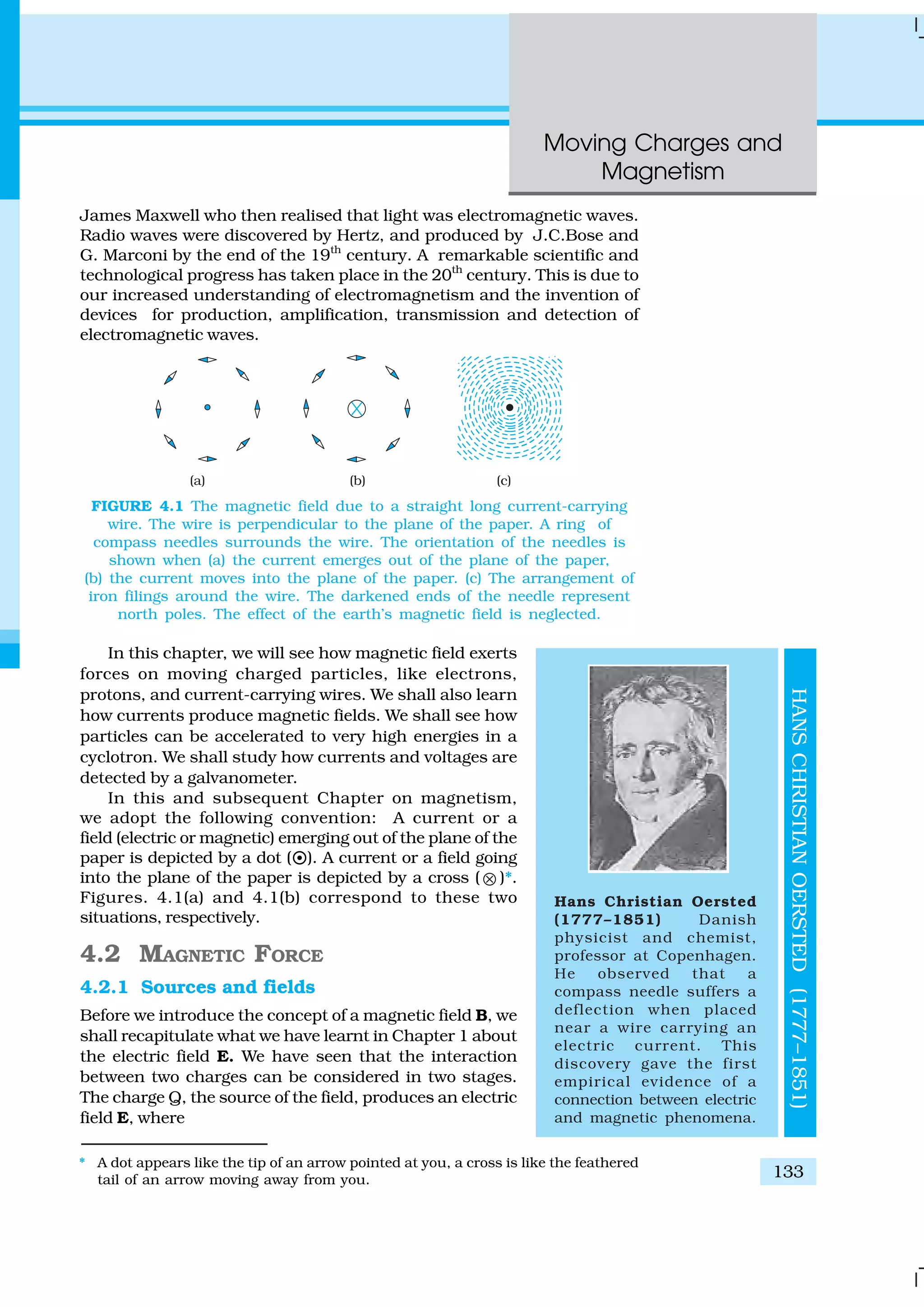
138. Physics
134
E = Q ˆr / (4πε0
)r2
(4.1)
where ˆr is unit vector along r, and the field E is a vector
field. A charge q interacts with this field and experiences
a force F given by
F = q E = q Q ˆr / (4πε0
) r2
(4.2)
As pointed out in the Chapter 1, the field E is not
just an artefact but has a physical role. It can convey
energy and momentum and is not established
instantaneously but takes finite time to propagate. The
concept of a field was specially stressed by Faraday and
was incorporated by Maxwell in his unification of
electricity and magnetism. In addition to depending on
each point in space, it can also vary with time, i.e., be a
function of time. In our discussions in this chapter, we
will assume that the fields do not change with time.
The field at a particular point can be due to one or
more charges. If there are more charges the fields add
vectorially. You have already learnt in Chapter 1 that this
is called the principle of superposition. Once the field is
known, the force on a test charge is given by Eq. (4.2).
Just as static charges produce an electric field, the
currents or moving charges produce (in addition) a
magnetic field, denoted by B (r), again a vector field. It
has several basic properties identical to the electric field.
It is defined at each point in space (and can in addition
depend on time). Experimentally, it is found to obey the
principle of superposition: the magnetic field of several
sources is the vector addition of magnetic field of each
individual source.
4.2.2 Magnetic Field, Lorentz Force
Let us suppose that there is a point charge q (moving
with a velocity v and, located at r at a given time t) in
presence of both the electric field E (r) and the magnetic
field B (r). The force on an electric charge q due to both of
them can be written as
F = q [ E (r) + v × B (r)] ≡ Felectric
+Fmagnetic
(4.3)
This force was given first by H.A. Lorentz based on the extensive
experiments of Ampere and others. It is called the Lorentz force. You
have already studied in detail the force due to the electric field. If we
look at the interaction with the magnetic field, we find the following
features.
(i) It depends on q, v and B (charge of the particle, the velocity and the
magnetic field). Force on a negative charge is opposite to that on a
positive charge.
(ii) The magnetic force q [ v × B ] includes a vector product of velocity
and magnetic field. The vector product makes the force due to magnetic
HENDRIKANTOONLORENTZ(1853–1928)
Hendrik Antoon Lorentz
(1853 – 1928) Dutch
theoretical physicist,
professor at Leiden. He
investigated the
relationship between
electricity, magnetism, and
mechanics. In order to
explain the observed effect
of magnetic fields on
emitters of light (Zeeman
effect), he postulated the
existence of electric charges
in the atom, for which he
was awarded the Nobel Prize
in 1902. He derived a set of
transformation equations
(known after him, as
Lorentz transformation
equations) by some tangled
mathematical arguments,
but he was not aware that
these equations hinge on a
new concept of space and
time.

139. Moving Charges and
Magnetism
135
field vanish (become zero) if velocity and magnetic field are parallel
or anti-parallel. The force acts in a (sideways) direction perpendicular
to both the velocity and the magnetic field.
Its direction is given by the screw rule or
right hand rule for vector (or cross) product
as illustrated in Fig. 4.2.
(iii) The magnetic force is zero if charge is not
moving (as then |v|= 0). Only a moving
charge feels the magnetic force.
The expression for the magnetic force helps
us to define the unit of the magnetic field, if
one takes q, F and v, all to be unity in the force
equation F = q [ v × B] =q v B sin θ ˆn , where θ
is the angle between v and B [see Fig. 4.2 (a)].
The magnitude of magnetic field B is 1 SI unit,
when the force acting on a unit charge (1 C),
moving perpendicular to B with a speed 1m/s,
is one newton.
Dimensionally, we have [B] = [F/qv] and the unit
of B are Newton second / (coulomb metre). This
unit is called tesla (T) named after Nikola Tesla
(1856 – 1943). Tesla is a rather large unit. A smaller unit (non-SI) called
gauss (=10–4
tesla) is also often used. The earth’s magnetic field is about
3.6 × 10–5
T. Table 4.1 lists magnetic fields over a wide range in the
universe.
FIGURE 4.2 The direction of the magnetic
force acting on a charged particle. (a) The
force on a positively charged particle with
velocity v and making an angle θ with the
magnetic field B is given by the right-hand
rule. (b) A moving charged particle q is
deflected in an opposite sense to –q in the
presence of magnetic field.
TABLE 4.1 ORDER OF MAGNITUDES OF MAGNETIC FIELDS IN A VARIETY OF PHYSICAL SITUATIONS
Physical situation Magnitude of B (in tesla)
Surface of a neutron star 108
Typical large field in a laboratory 1
Near a small bar magnet 10–2
On the earth’s surface 10–5
Human nerve fibre 10–10
Interstellar space 10–12
4.2.3 Magnetic force on a current-carrying conductor
We can extend the analysis for force due to magnetic field on a single
moving charge to a straight rod carrying current. Consider a rod of a
uniform cross-sectional area A and length l. We shall assume one kind
of mobile carriers as in a conductor (here electrons). Let the number
density of these mobile charge carriers in it be n. Then the total number
of mobile charge carriers in it is nAl. For a steady current I in this
conducting rod, we may assume that each mobile carrier has an average

140. Physics
136
EXAMPLE4.1
drift velocity vd
(see Chapter 3). In the presence of an external magnetic
field B, the force on these carriers is:
F = (nAl)q vd
× B
where q is the value of the charge on a carrier. Now nqvd
is the current
density j and |(nq vd
)|A is the current I (see Chapter 3 for the discussion
of current and current density). Thus,
F = [(nqevd
)Al] × B = [ jAl ] × B
= I1 × B (4.4)
where l is a vector of magnitude l, the length of the rod, and with a direction
identical to the current I. Note that the current I is not a vector. In the last
step leading to Eq. (4.4), we have transferred the vector sign from j to l.
Equation (4.4) holds for a straight rod. In this equation, B is the external
magnetic field. It is not the field produced by the current-carrying rod. If
the wire has an arbitrary shape we can calculate the Lorentz force on it
by considering it as a collection of linear strips dlj
and summing
d j
j
I= ∑F l × B
This summation can be converted to an integral in most cases.
ON PERMITTIVITY AND PERMEABILITY
In the universal law of gravitation, we say that any two point masses exert a force on
each other which is proportional to the product of the masses m1
, m2
and inversely
proportional to the square of the distance r between them. We write it as F = Gm1
m2
/r2
where G is the universal constant of gravitation. Similarly in Coulomb’s law of electrostatics
we write the force between two point charges q1
, q2
, separated by a distance r as
F = kq1
q2
/r2
where k is a constant of proportionality. In SI units, k is taken as
1/4πε where ε is the permittivity of the medium. Also in magnetism, we get another
constant, which in SI units, is taken as µ/4π where µ is the permeability of the medium.
Although G, ε and µ arise as proportionality constants, there is a difference between
gravitational force and electromagnetic force. While the gravitational force does not depend
on the intervening medium, the electromagnetic force depends on the medium between
the two charges or magnets. Hence while G is a universal constant, ε and µ depend on
the medium. They have different values for different media. The product εµ turns out to
be related to the speed v of electromagnetic radiation in the medium through εµ =1/ v 2
.
Electric permittivity ε is a physical quantity that describes how an electric field affects
and is affected by a medium. It is determined by the ability of a material to polarise in
response to an applied field, and thereby to cancel, partially, the field inside the material.
Similarly, magnetic permeability µ is the ability of a substance to acquire magnetisation in
magnetic fields. It is a measure of the extent to which magnetic field can penetrate matter.
Example 4.1 A straight wire of mass 200 g and length 1.5 m carries
a current of 2 A. It is suspended in mid-air by a uniform horizontal
magnetic field B (Fig. 4.3). What is the magnitude of the magnetic
field?

141. Moving Charges and
Magnetism
137
EXAMPLE4.1
FIGURE 4.3
Solution From Eq. (4.4), we find that there is an upward force F, of
magnitude IlB,. For mid-air suspension, this must be balanced by
the force due to gravity:
m g = I lB
m g
B
I l
=
0.2 9.8
0.65 T
2 1.5
×
= =
×
Note that it would have been sufficient to specify m/l, the mass per
unit length of the wire. The earth’s magnetic field is approximately
4 × 10–5
T and we have ignored it.
Example 4.2 If the magnetic field is parallel to the positive y-axis
and the charged particle is moving along the positive x-axis (Fig. 4.4),
which way would the Lorentz force be for (a) an electron (negative
charge), (b) a proton (positive charge).
FIGURE 4.4
Solution The velocity v of particle is along the x-axis, while B, the
magnetic field is along the y-axis, so v × B is along the z-axis (screw
rule or right-hand thumb rule). So, (a) for electron it will be along –z
axis. (b) for a positive charge (proton) the force is along +z axis.
4.3 MOTION IN A MAGNETIC FIELD
We will now consider, in greater detail, the motion of a charge moving in
a magnetic field. We have learnt in Mechanics (see Class XI book, Chapter
6) that a force on a particle does work if the force has a component along
(or opposed to) the direction of motion of the particle. In the case of motion
EXAMPLE4.2
Chargedparticlesmovinginamagneticfield.
Interactivedemonstration:
http://www.phys.hawaii.edu/~teb/optics/java/partmagn/index.html

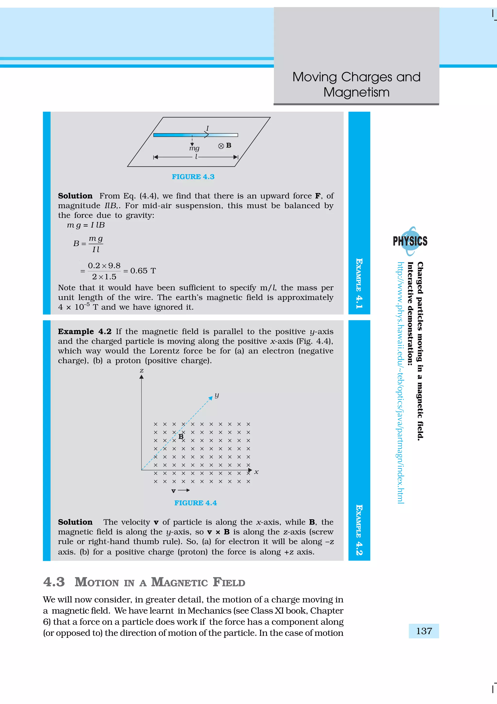
142. Physics
138
of a charge in a magnetic field, the magnetic force is
perpendicular to the velocity of the particle. So no work is done
and no change in the magnitude of the velocity is produced
(though the direction of momentum may be changed). [Notice
that this is unlike the force due to an electric field, qE, which
can have a component parallel (or antiparallel) to motion and
thus can transfer energy in addition to momentum.]
We shall consider motion of a charged particle in a uniform
magnetic field. First consider the case of v perpendicular to B.
The perpendicular force, q v × B, acts as a centripetal force and
produces a circular motion perpendicular to the magnetic field.
The particle will describe a circle if v and B are perpendicular
to each other (Fig. 4.5).
If velocity has a component along B, this component
remains unchanged as the motion along the magnetic field will
not be affected by the magnetic field. The motion
in a plane perpendicular to B is as before a
circular one, thereby producing a helical motion
(Fig. 4.6).
You have already learnt in earlier classes
(See Class XI, Chapter 4) that if r is the radius
of the circular path of a particle, then a force of
m v2
/ r, acts perpendicular to the path towards
the centre of the circle, and is called the
centripetal force. If the velocity v is
perpendicular to the magnetic field B, the
magnetic force is perpendicular to both v and
B and acts like a centripetal force. It has a
magnitude q v B. Equating the two expressions
for centripetal force,
m v 2
/r = q v B, which gives
r = m v / qB (4.5)
for the radius of the circle described by the
charged particle. The larger the momentum,
the larger is the radius and bigger the circle described. If ω is the angular
frequency, then v = ω r. So,
ω = 2π ν = q B/ m [4.6(a)]
which is independent of the velocity or energy . Here ν is the frequency of
rotation. The independence of ν from energy has important application
in the design of a cyclotron (see Section 4.4.2).
The time taken for one revolution is T= 2π/ω ≡ 1/ν. If there is a
component of the velocity parallel to the magnetic field (denoted by v||
), it
will make the particle move along the field and the path of the particle
would be a helical one (Fig. 4.6). The distance moved along the magnetic
field in one rotation is called pitch p. Using Eq. [4.6 (a)], we have
p = v||
T = 2πm v||
/ q B [4.6(b)]
The radius of the circular component of motion is called the radius of
the helix.
FIGURE 4.5 Circular motion
FIGURE 4.6 Helical motion

143. Moving Charges and
Magnetism
139
EXAMPLE4.3
Example 4.3 What is the radius of the path of an electron (mass
9 × 10-31
kg and charge 1.6 × 10–19
C) moving at a speed of 3 ×107
m/s in
a magnetic field of 6 × 10–4
T perpendicular to it? What is its
frequency? Calculate its energy in keV. ( 1 eV = 1.6 × 10–19
J).
Solution Using Eq. (4.5) we find
r = m v / (qB) = 9 ×10–31
kg × 3 × 107
m s–1
/ ( 1.6 × 10–19
C × 6 × 10–4
T)
= 26 × 10–2
m = 26 cm
ν = v / (2 πr) = 2×106
s–1
= 2×106
Hz =2 MHz.
E = (½ )mv 2
= (½ ) 9 × 10–31
kg × 9 × 1014
m2
/s2
= 40.5 ×10–17
J
≈ 4×10–16
J = 2.5 keV.
HELICAL MOTION OF CHARGED PARTICLES AND AURORA BORIOLIS
In polar regions like Alaska and Northern Canada, a splendid display of colours is seen
in the sky. The appearance of dancing green pink lights is fascinating, and equally
puzzling. An explanation of this natural phenomenon is now found in physics, in terms
of what we have studied here.
Consider a charged particle of mass m and charge q, entering a region of magnetic
field B with an initial velocity v. Let this velocity have a component vp
parallel to the
magnetic field and a component vn
normal to it. There is no force on a charged particle in
the direction of the field. Hence the particle continues to travel with the velocity vp
parallel
to the field. The normal component vn
of the particle results in a Lorentz force (vn
× B)
which is perpendicular to both vn
and B. As seen in Section 4.3.1 the particle thus has a
tendency to perform a circular motion in a plane perpendicular to the magnetic field.
When this is coupled with the velocity parallel to the field, the resulting trajectory will be
a helix along the magnetic field line, as shown in Figure (a) here. Even if the field line
bends, the helically moving particle is trapped and guided to move around the field line.
Since the Lorentz force is normal to the velocity of each point, the field does no work on
the particle and the magnitude of velocity remains the same.
During a solar flare, a large number of electrons and protons are ejected from the sun.
Some of them get trapped in the earth’s magnetic field and move in helical paths along the
field lines. The field lines come closer to each other near the magnetic poles; see figure (b).
Hence the density of charges increases near the poles. These particles collide with atoms
and molecules of the atmosphere. Excited oxygen atoms emit green light and excited
nitrogen atoms emits pink light. This phenomenon is called Aurora Boriolis in physics.

144. Physics
140
4.4 MOTION IN COMBINED ELECTRIC AND MAGNETIC
FIELDS
4.4.1 Velocity selector
You know that a charge q moving with velocity v in presence of both
electric and magnetic fields experiences a force given by Eq. (4.3), that is,
F = q (E + v × B) = FE
+ FB
We shall consider the simple case in which electric and magnetic
fields are perpendicular to each other and also perpendicular to
the velocity of the particle, as shown in Fig. 4.7. We have,
ˆ ˆ ˆ, ,E B v= = =E j B k v i
( )ˆ ˆ ˆ ˆ, , –E Bq qE q q v B qB= = = = =F E j F v × B i × k j
Therefore, ( )ˆ–q E vB=F j .
Thus, electric and magnetic forces are in opposite directions as
shown in the figure. Suppose, we adjust the value of E and B such
that magnitude of the two forces are equal. Then, total force on the
charge is zero and the charge will move in the fields undeflected.
This happens when,
or
E
qE qvB v
B
= = (4.7)
This condition can be used to select charged particles of a particular
velocity out of a beam containing charges moving with different speeds
(irrespective of their charge and mass). The crossed E and B fields, therefore,
serve as a velocity selector. Only particles with speed E/B pass
undeflected through the region of crossed fields. This method was
employed by J. J. Thomson in 1897 to measure the charge to mass ratio
(e/m) of an electron. The principle is also employed in Mass Spectrometer –
a device that separates charged particles, usually ions, according to their
charge to mass ratio.
4.4.2 Cyclotron
The cyclotron is a machine to accelerate charged particles or ions to high
energies. It was invented by E.O. Lawrence and M.S. Livingston in 1934
to investigate nuclear structure. The cyclotron uses both electric and
magnetic fields in combination to increase the energy of charged particles.
As the fields are perpendicular to each other they are called crossed
fields. Cyclotron uses the fact that the frequency of revolution of the
charged particle in a magnetic field is independent of its energy. The
particles move most of the time inside two semicircular disc-like metal
containers, D1
and D2
, which are called dees as they look like the letter
D. Figure 4.8 shows a schematic view of the cyclotron. Inside the metal
boxes the particle is shielded and is not acted on by the electric field. The
magnetic field, however, acts on the particle and makes it go round in a
circular path inside a dee. Every time the particle moves from one dee to
another it is acted upon by the electric field. The sign of the electric field
is changed alternately in tune with the circular motion of the particle.
This ensures that the particle is always accelerated by the electric field.
Each time the acceleration increases the energy of the particle. As energy
FIGURE 4.7
Cyclotron
Interactivedemonstration:
http://www.phy.ntnu.edu.tw/ntnujava/viewtopic.php?t=50

145. Moving Charges and
Magnetism
141
increases, the radius of the circular path increases. So the path is a
spiral one.
The whole assembly is evacuated to minimise collisions between the
ions and the air molecules. A high frequency alternating voltage is applied
to the dees. In the sketch shown in Fig. 4.8, positive ions or positively
charged particles (e.g., protons) are released at the centre P. They move
in a semi-circular path in one of the dees and arrive in the gap between
the dees in a time interval T/2; where T, the period of revolution, is given
by Eq. (4.6),
1 2
c
m
T
qBν
π
= =
or
2
c
qB
m
ν =
π
(4.8)
This frequency is called the cyclotron frequency for obvious reasons
and is denoted by νc
.
The frequency νa
of the applied voltage is adjusted so that the polarity
of the dees is reversed in the same time that it takes the ions to complete
one half of the revolution. The requirement νa
= νc
is called the resonance
condition. The phase of the supply is adjusted so that when the positive
ions arrive at the edge of D1
, D2
is at a lower
potential and the ions are accelerated across the
gap. Inside the dees the particles travel in a region
free of the electric field. The increase in their
kinetic energy is qV each time they cross from
one dee to another (V refers to the voltage across
the dees at that time). From Eq. (4.5), it is clear
that the radius of their path goes on increasing
each time their kinetic energy increases. The ions
are repeatedly accelerated across the dees until
they have the required energy to have a radius
approximately that of the dees. They are then
deflected by a magnetic field and leave the system
via an exit slit. From Eq. (4.5) we have,
qBR
v
m
= (4.9)
where R is the radius of the trajectory at exit, and
equals the radius of a dee.
Hence, the kinetic energy of the ions is,
2 2 2
21
2 2
q B R
m
m
=v (4.10)
The operation of the cyclotron is based on the
fact that the time for one revolution of an ion is
independent of its speed or radius of its orbit.
The cyclotron is used to bombard nuclei with
energetic particles, so accelerated by it, and study
FIGURE 4.8 A schematic sketch of the
cyclotron. There is a source of charged
particles or ions at P which move in a
circular fashion in the dees, D1
and D2
, on
account of a uniform perpendicular
magnetic field B. An alternating voltage
source accelerates these ions to high
speeds. The ions are eventually ‘extracted’
at the exit port.

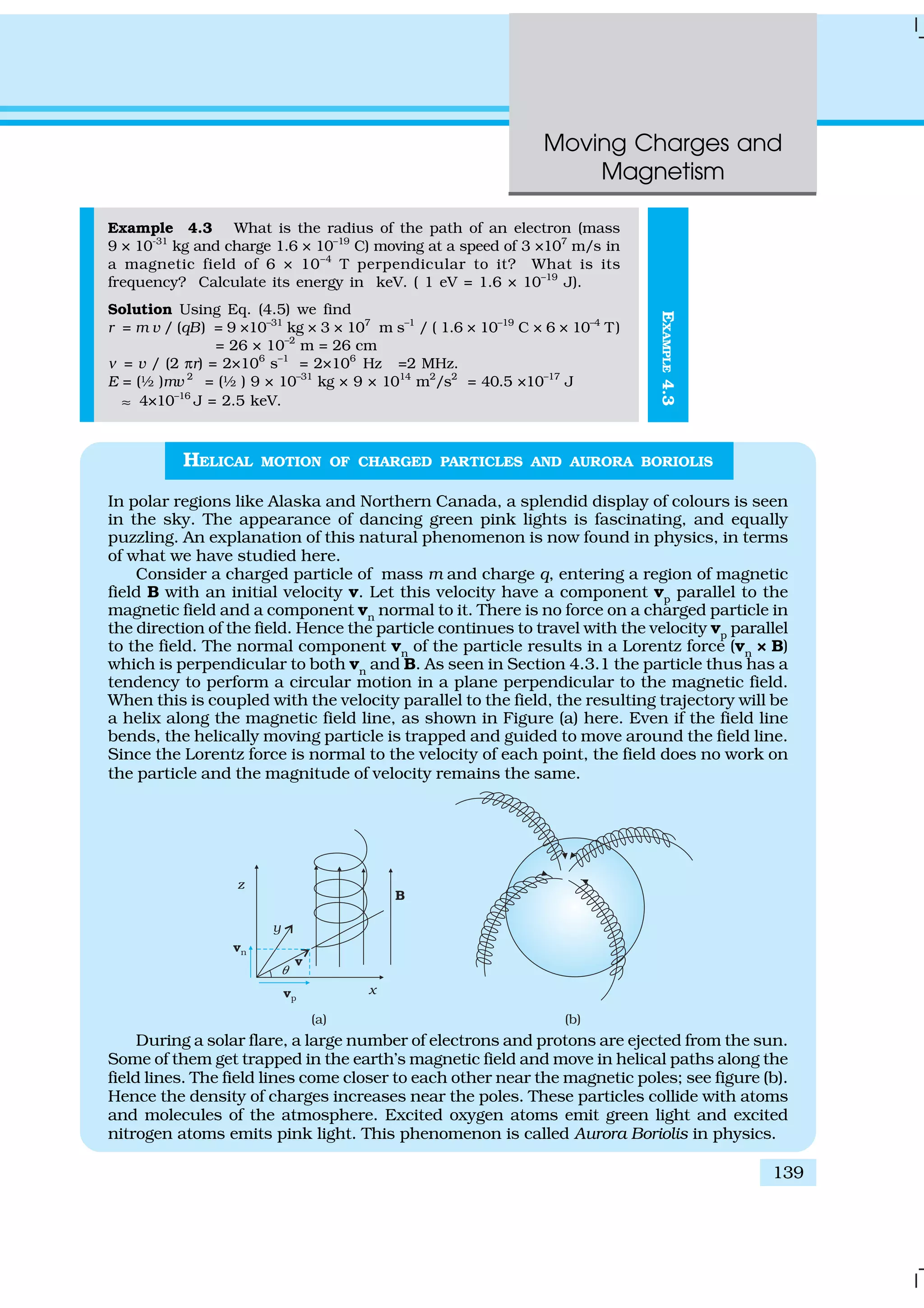
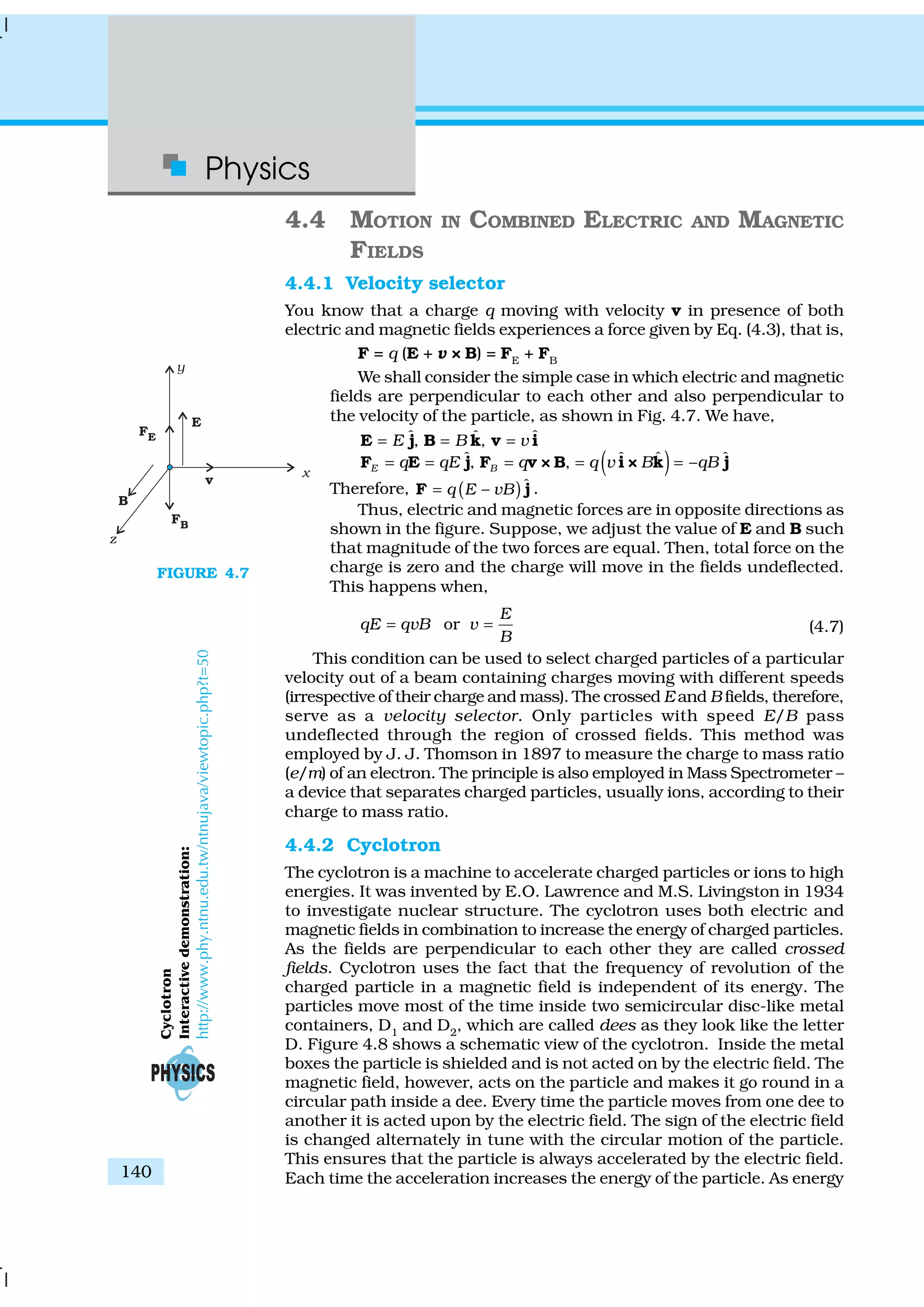
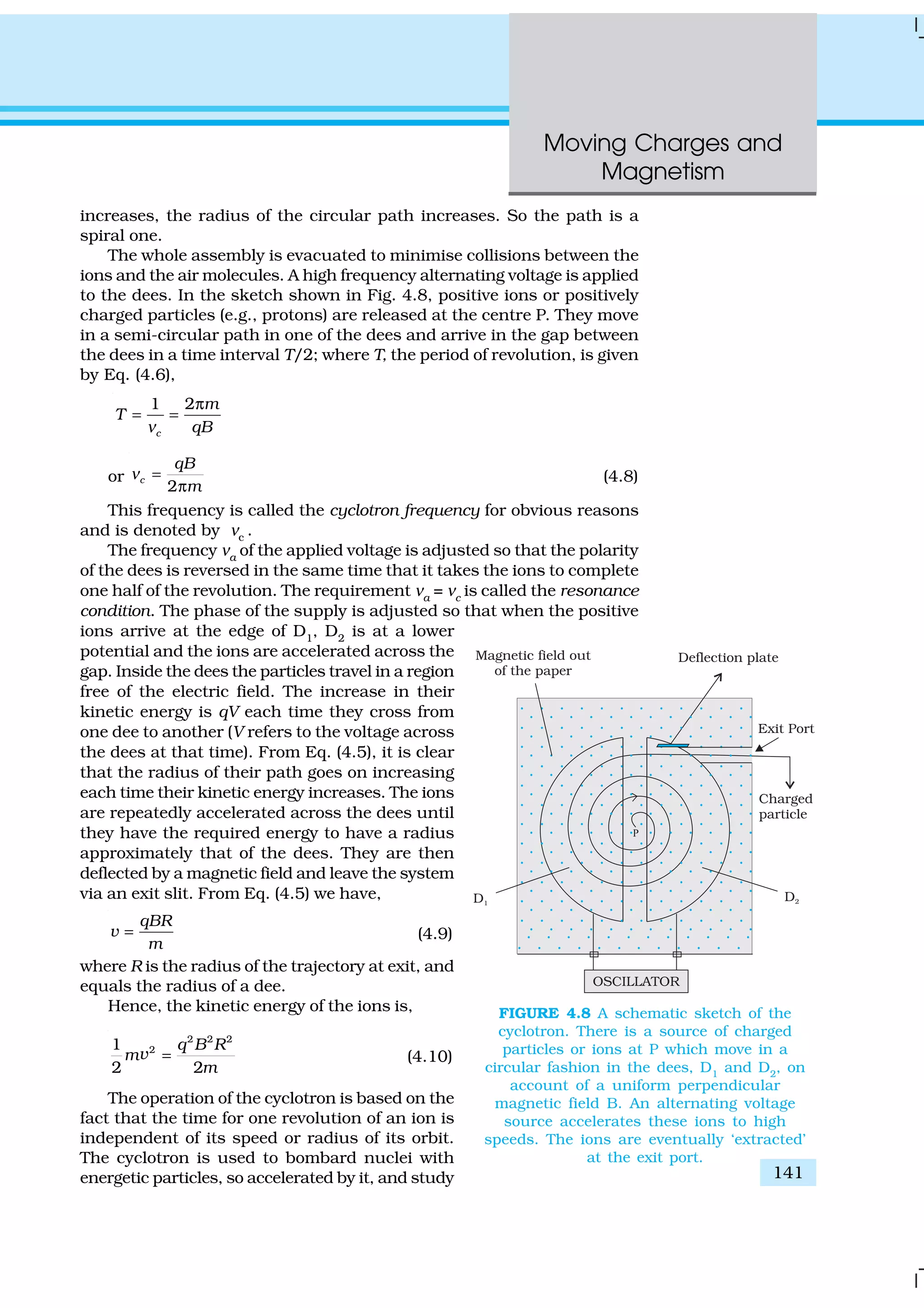
146. Physics
142
EXAMPLE4.4
the resulting nuclear reactions. It is also used to implant ions into solids
and modify their properties or even synthesise new materials. It is used
in hospitals to produce radioactive substances which can be used in
diagnosis and treatment.
Example 4.4 A cyclotron’s oscillator frequency is 10 MHz. What
should be the operating magnetic field for accelerating protons? If
the radius of its ‘dees’ is 60 cm, what is the kinetic energy (in MeV) of
the proton beam produced by the accelerator.
(e =1.60 × 10–19
C, mp
= 1.67 × 10–27
kg, 1 MeV = 1.6 × 10–13
J).
Solution The oscillator frequency should be same as proton’s
cyclotron frequency.
Using Eqs. (4.5) and [4.6(a)] we have
B = 2π m ν/q =6.3 ×1.67 × 10–27
× 107
/ (1.6 × 10–19
) = 0.66 T
Final velocity of protons is
v = r × 2π ν = 0.6 m × 6.3 ×107
= 3.78 × 107
m/s.
E = ½ mv 2
= 1.67 ×10–27
× 14.3 × 1014
/ (2 × 1.6 × 10–13
) = 7 MeV.
ACCELERATORS IN INDIA
India has been an early entrant in the area of accelerator- based research. The vision of
Dr. Meghnath Saha created a 37" Cyclotron in the Saha Institute of Nuclear Physics in
Kolkata in 1953. This was soon followed by a series of Cockroft-Walton type of accelerators
established in Tata Institute of Fundamental Research (TIFR), Mumbai, Aligarh Muslim
University (AMU), Aligarh, Bose Institute, Kolkata and Andhra University, Waltair.
The sixties saw the commissioning of a number of Van de Graaff accelerators: a 5.5 MV
terminal machine in Bhabha Atomic Research Centre (BARC), Mumbai (1963); a 2 MV terminal
machine in Indian Institute of Technology (IIT), Kanpur; a 400 kV terminal machine in Banaras
Hindu University (BHU), Varanasi; and Punjabi University, Patiala. One 66 cm Cyclotron
donated by the Rochester University of USA was commissioned in Panjab University,
Chandigarh. A small electron accelerator was also established in University of Pune, Pune.
In a major initiative taken in the seventies and eighties, a Variable Energy Cyclotron was
built indigenously in Variable Energy Cyclotron Centre (VECC), Kolkata; 2 MV Tandem Van
de Graaff accelerator was developed and built in BARC and a 14 MV Tandem Pelletron
accelerator was installed in TIFR.
This was soon followed by a 15 MV Tandem Pelletron established by University Grants
Commission (UGC), as an inter-university facility in Inter-University Accelerator Centre
(IUAC), New Delhi; a 3 MV Tandem Pelletron in Institute of Physics, Bhubaneshwar; and
two 1.7 MV Tandetrons in Atomic Minerals Directorate for Exploration and Research,
Hyderabad and Indira Gandhi Centre for Atomic Research, Kalpakkam. Both TIFR and
IUAC are augmenting their facilities with the addition of superconducting LINAC modules
to accelerate the ions to higher energies.
Besides these ion accelerators, the Department of Atomic Energy (DAE) has developed
many electron accelerators. A 2 GeV Synchrotron Radiation Source is being built in Raja
Ramanna Centre for Advanced Technologies, Indore.
The Department of Atomic Energy is considering Accelerator Driven Systems (ADS) for
power production and fissile material breeding as future options.

147. Moving Charges and
Magnetism
143
4.5 MAGNETIC FIELD DUE TO A CURRENT ELEMENT,
BIOT-SAVART LAW
All magnetic fields that we know are due to currents (or moving charges)
and due to intrinsic magnetic moments of particles. Here, we shall study
the relation between current and the magnetic field it produces.
It is given by the Biot-Savart’s law. Figure 4.9 shows a finite
conductor XY carrying current I. Consider an infinitesimal
element dl of the conductor. The magnetic field dB due to this
element is to be determined at a point P which is at a distance r
from it. Let θ be the angle between dl and the displacement vector
r. According to Biot-Savart’s law, the magnitude of the magnetic
field dB is proportional to the current I, the element length |dl|,
and inversely proportional to the square of the distance r. Its
direction* is perpendicular to the plane containing dl and r .
Thus, in vector notation,
3
I d
d
r
×
∝
l r
B
0
3
4
I d
r
µ ×
=
π
l r
[4.11(a)]
where µ0
/4π is a constant of proportionality. The above
expression holds when the medium is vacuum.
The magnitude of this field is,
0
2
d sin
d
4
I l
r
µ θ
=
π
B [4.11(b)]
where we have used the property of cross-product. Equation [4.11 (a)]
constitutes our basic equation for the magnetic field. The proportionality
constant in SI units has the exact value,
70
10 Tm/A
4
µ −
=
π
[4.11(c)]
We call µ0
the permeability of free space (or vacuum).
The Biot-Savart law for the magnetic field has certain similarities as
well as differences with the Coulomb’s law for the electrostatic field. Some
of these are:
(i) Both are long range, since both depend inversely on the square of
distance from the source to the point of interest. The principle of
superposition applies to both fields. [In this connection, note that
the magnetic field is linear in the source I dl just as the electrostatic
field is linear in its source: the electric charge.]
(ii) The electrostatic field is produced by a scalar source, namely, the
electric charge. The magnetic field is produced by a vector source
I dl.
* The sense of dl×r is also given by the Right Hand Screw rule : Look at the plane
containing vectors dl and r. Imagine moving from the first vector towards second
vector. If the movement is anticlockwise, the resultant is towards you. If it is
clockwise, the resultant is away from you.
FIGURE 4.9 Illustration of
the Biot-Savart law. The
current element I dl
produces a field dB at a
distance r. The ⊗ sign
indicates that the
field is perpendicular
to the plane of this
page and directed
into it.

148. Physics
144
EXAMPLE4.5
(iii) The electrostatic field is along the displacement vector joining the
source and the field point. The magnetic field is perpendicular to the
plane containing the displacement vector rand the current element
I dl.
(iv) There is an angle dependence in the Biot-Savart law which is not
present in the electrostatic case. In Fig. 4.9, the magnetic field at any
point in the direction of dl (the dashed line) is zero. Along this line,
θ = 0, sin θ = 0 and from Eq. [4.11(a)], |dB| = 0.
There is an interesting relation between ε0
, the permittivity of free
space; µ0
, the permeability of free space; and c, the speed of light in
vacuum:
( ) 0
0 0 04
4
µ
ε µ ε
 
= π   π
( )7
9
1
10
9 10
− 
=   × 8 2 2
1 1
(3 10 ) c
= =
×
We will discuss this connection further in Chapter 8 on the
electromagnetic waves. Since the speed of light in vacuum is constant,
the product µ0
ε0
is fixed in magnitude. Choosing the value of either ε0
or
µ0
, fixes the value of the other. In SI units, µ0
is fixed to be equal to
4π × 10–7
in magnitude.
Example 4.5 An element ˆx∆ = ∆l i is placed at the origin and carries
a large current I = 10 A (Fig. 4.10). What is the magnetic field on the
y-axis at a distance of 0.5 m. ∆x = 1 cm.
FIGURE 4.10
Solution
0
2
d sin
|d |
4
I l
r
µ θ
=
π
B [using Eq. (4.11)]
2
d 10 ml x −
= ∆ = , I = 10 A, r = 0.5 m = y, 7
0
T m
/4 10
A
µ −
π =
θ = 90° ; sin θ = 1
7 2
2
10 10 10
d
25 10
− −
−
× ×
=
×
B = 4 × 10–8
T
The direction of the field is in the +z-direction. This is so since,
ˆ ˆd x y= ∆l × i × jr ( )ˆ ˆy x= ∆ i × j ˆy x= ∆ k
We remind you of the following cyclic property of cross-products,
ˆ ˆ ˆ ˆ ˆ ˆ ˆ ˆ ˆ; ;× = × = × =i j k j k i k i j
Note that the field is small in magnitude.

149. Moving Charges and
Magnetism
145
In the next section, we shall use the Biot-Savart law to calculate the
magnetic field due to a circular loop.
4.6 MAGNETIC FIELD ON THE AXIS OF A CIRCULAR
CURRENT LOOP
In this section, we shall evaluate the magnetic field due to a circular coil
along its axis. The evaluation entails summing up the effect of infinitesimal
current elements (I dl) mentioned in the previous section.
We assume that the current I is steady and that the
evaluation is carried out in free space (i.e., vacuum).
Figure 4.11 depicts a circular loop carrying a steady
current I. The loop is placed in the y-z plane with its
centre at the origin O and has a radius R. The x-axis is
the axis of the loop. We wish to calculate the magnetic
field at the point P on this axis. Let x be the distance of
P from the centre O of the loop.
Consider a conducting element dl of the loop. This is
shown in Fig. 4.11. The magnitude dB of the magnetic
field due to dl is given by the Biot-Savart law [Eq. 4.11(a)],
0
3
4
I d
dB
r
µ
π
=
l × r
(4.12)
Now r2
= x2
+ R2
. Further, any element of the loop
will be perpendicular to the displacement vector from
the element to the axial point. For example, the element
dl in Fig. 4.11 is in the y-z plane whereas the
displacement vector r from dl to the axial point P is in
the x-y plane. Hence |dl × r|=r dl. Thus,
( )ð
0
2 2
d
d
4
I l
B
x R
µ
=
+ (4.13)
The direction of dB is shown in Fig. 4.11. It is perpendicular to the
plane formed by dl and r. It has an x-component dBx
and a component
perpendicular to x-axis, dB⊥
. When the components perpendicular to
the x-axis are summed over, they cancel out and we obtain a null result.
For example, the dB⊥
component due to dl is cancelled by the
contribution due to the diametrically opposite dl element, shown in
Fig. 4.11. Thus, only the x-component survives. The net contribution
along x-direction can be obtained by integrating dBx
= dB cos θ over the
loop. For Fig. 4.11,
2 2 1/2
cos
( )
R
x R
θ =
+
(4.14)
From Eqs. (4.13) and (4.14),
( )ð
0
3/22 2
d
d
4
x
I l R
B
x R
µ
=
+
FIGURE 4.11 Magnetic field on the
axis of a current carrying circular
loop of radius R. Shown are the
magnetic field dB (due to a line
element dl ) and its
components along and
perpendicular to the axis.

150. Physics
146
EXAMPLE4.6
The summation of elements dl over the loop yields 2πR, the
circumference of the loop. Thus, the magnetic field at P due to entire
circular loop is
( )
2
0
3/22 2
ˆ ˆ
2
x
I R
B
x R
µ
= =
+
B i i (4.15)
As a special case of the above result, we may obtain the field at the centre
of the loop. Here x = 0, and we obtain,
0
0
ˆ
2
I
R
µ
=B i (4.16)
The magnetic field lines due to a circular wire form closed loops and
are shown in Fig. 4.12. The direction of the magnetic field is given by
(another) right-hand thumb rule stated below:
Curl the palm of your right hand around the circular wire with the
fingers pointing in the direction of the current. The right-hand thumb
gives the direction of the magnetic field.
Example 4.6 A straight wire carrying a current of 12 A is bent into a
semi-circular arc of radius 2.0 cm as shown in Fig. 4.13(a). Consider
the magnetic field B at the centre of the arc. (a) What is the magnetic
field due to the straight segments? (b) In what way the contribution
to B from the semicircle differs from that of a circular loop and in
what way does it resemble? (c) Would your answer be different if the
wire were bent into a semi-circular arc of the same radius but in the
opposite way as shown in Fig. 4.13(b)?
FIGURE 4.13
FIGURE 4.12 The magnetic field lines for a current loop. The direction of
the field is given by the right-hand thumb rule described in the text. The
upper side of the loop may be thought of as the north pole and the lower
side as the south pole of a magnet.

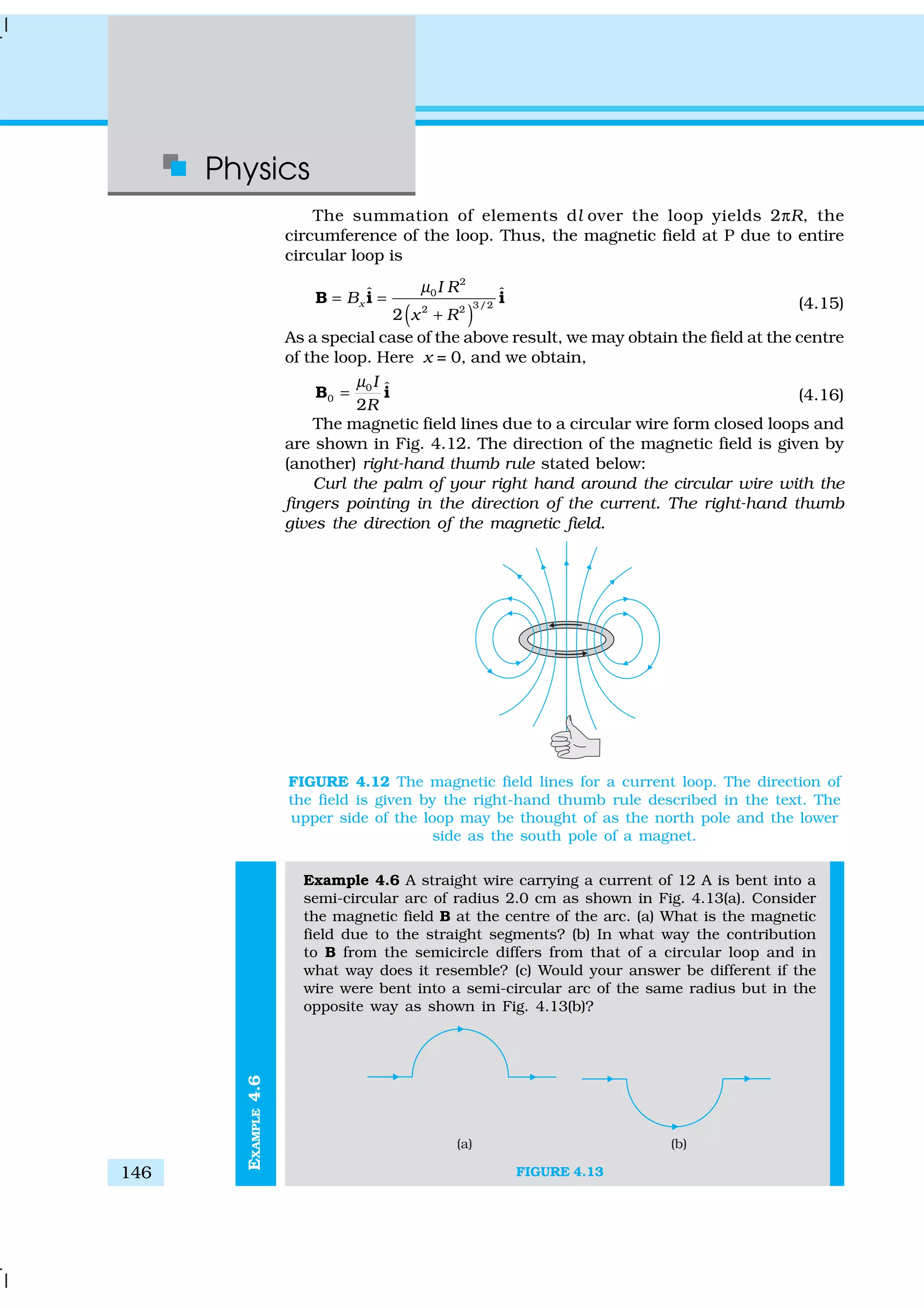
151. Moving Charges and
Magnetism
147
EXAMPLE4.6
Solution
(a) dl and r for each element of the straight segments are parallel.
Therefore, dl × r = 0. Straight segments do not contribute to
|B|.
(b) For all segments of the semicircular arc, dl × r are all parallel to
each other (into the plane of the paper). All such contributions
add up in magnitude. Hence direction of B for a semicircular arc
is given by the right-hand rule and magnitude is half that of a
circular loop. Thus B is 1.9 × 10–4
T normal to the plane of the
paper going into it.
(c) Same magnitude of B but opposite in direction to that in (b).
Example 4.7 Consider a tightly wound 100 turn coil of radius 10 cm,
carrying a current of 1 A. What is the magnitude of the magnetic
field at the centre of the coil?
Solution Since the coil is tightly wound, we may take each circular
element to have the same radius R = 10 cm = 0.1 m. The number of
turns N = 100. The magnitude of the magnetic field is,
–7 2
0
–1
4 10 10 1
2 2 10
NI
B
R
µ π × × ×
= =
×
4
2 10−
= π ×
4
6 28 10 T. −
= ×
4.7 AMPERE’S CIRCUITAL LAW
There is an alternative and appealing way in which the Biot-Savart law
may be expressed. Ampere’s circuital law considers an open surface
with a boundary (Fig. 4.14). The surface has current passing
through it. We consider the boundary to be made up of a number
of small line elements. Consider one such element of length dl. We
take the value of the tangential component of the magnetic field,
Bt
, at this element and multiply it by the length of that element dl
[Note: Bt
dl=B.dl]. All such products are added together. We
consider the limit as the lengths of elements get smaller and their
number gets larger. The sum then tends to an integral. Ampere’s
law states that this integral is equal to µ0
times the total current
passing through the surface, i.e.,
0d Iµ=∫ B lgÑ [4.17(a)]
where I is the total current through the surface. The integral is taken
over the closed loop coinciding with the boundary C of the surface. The
relation above involves a sign-convention, given by the right-hand rule.
Let the fingers of the right-hand be curled in the sense the boundary is
traversed in the loop integral “B.dl. Then the direction of the thumb
gives the sense in which the current I is regarded as positive.
For several applications, a much simplified version of Eq. [4.17(a)]
proves sufficient. We shall assume that, in such cases, it is possible to
choose the loop (called an amperian loop) such that at each point of the
loop, either
FIGURE 4.14
EXAMPLE4.7

152. Physics
148
(i) B is tangential to the loop and is a non-zero constant
B, or
(ii) B is normal to the loop, or
(iii) B vanishes.
Now, let L be the length (part) of the loop for which B
is tangential. Let Ie
be the current enclosed by the loop.
Then, Eq. (4.17) reduces to,
BL =µ0
Ie
[4.17(b)]
When there is a system with a symmetry such as for
a straight infinite current-carrying wire in Fig. 4.15, the
Ampere’s law enables an easy evaluation of the magnetic
field, much the same way Gauss’ law helps in
determination of the electric field. This is exhibited in the
Example 4.8 below. The boundary of the loop chosen is
a circle and magnetic field is tangential to the
circumference of the circle. The law gives, for the left hand
side of Eq. [4.17 (b)], B. 2πr. We find that the magnetic
field at a distance r outside the wire is tangential and
given by
B × 2πr = µ0
I,
B = µ0
I/ (2πr) (4.18)
The above result for the infinite wire is interesting
from several points of view.
(i) It implies that the field at every point on a circle of
radius r, (with the wire along the axis), is same in
magnitude. In other words, the magnetic field
possesses what is called a cylindrical symmetry. The
field that normally can depend on three coordinates
depends only on one: r. Whenever there is symmetry,
the solutions simplify.
(ii) The field direction at any point on this circle is
tangential to it. Thus, the lines of constant magnitude
of magnetic field form concentric circles. Notice now,
in Fig. 4.1(c), the iron filings form concentric circles.
These lines called magnetic field lines form closed
loops. This is unlike the electrostatic field lines which
originate from positive charges and end at negative
charges. The expression for the magnetic field of a
straight wire provides a theoretical justification to
Oersted’s experiments.
(iii) Another interesting point to note is that even though
the wire is infinite, the field due to it at a nonzero
distance is not infinite. It tends to blow up only when
we come very close to the wire. The field is directly
proportional to the current and inversely proportional
to the distance from the (infinitely long) current
source.
ANDREAMPERE(1775–1836)
Andre Ampere (1775 –
1836) Andre Marie Ampere
was a French physicist,
mathematician and
chemist who founded the
science of electrodynamics.
Ampere was a child prodigy
who mastered advanced
mathematics by the age of
12. Ampere grasped the
significance of Oersted’s
discovery. He carried out a
large series of experiments
to explore the relationship
between current electricity
and magnetism. These
investigations culminated
in 1827 with the
publication of the
‘Mathematical Theory of
Electrodynamic Pheno-
mena Deduced Solely from
Experiments’. He hypo-
thesised that all magnetic
phenomena are due to
circulating electric
currents. Ampere was
humble and absent-
minded. He once forgot an
invitation to dine with the
Emperor Napoleon. He died
of pneumonia at the age of
61. His gravestone bears
the epitaph: Tandem Felix
(Happy at last).

153. Moving Charges and
Magnetism
149
EXAMPLE4.8
(iv) There exists a simple rule to determine the direction of the magnetic
field due to a long wire. This rule, called the right-hand rule*, is:
Grasp the wire in your right hand with your extended thumb pointing
in the direction of the current. Your fingers will curl around in the
direction of the magnetic field.
Ampere’s circuital law is not new in content from Biot-Savart law.
Both relate the magnetic field and the current, and both express the same
physical consequences of a steady electrical current. Ampere’s law is to
Biot-Savart law, what Gauss’s law is to Coulomb’s law. Both, Ampere’s
and Gauss’s law relate a physical quantity on the periphery or boundary
(magnetic or electric field) to another physical quantity, namely, the source,
in the interior (current or charge). We also note that Ampere’s circuital
law holds for steady currents which do not fluctuate with time. The
following example will help us understand what is meant by the term
enclosed current.
Example 4.8 Figure 4.15 shows a long straight wire of a circular
cross-section (radius a) carrying steady current I. The current I is
uniformly distributed across this cross-section. Calculate the
magnetic field in the region r < a and r > a.
FIGURE 4.15
Solution (a) Consider the case r > a. The Amperian loop, labelled 2,
is a circle concentric with the cross-section. For this loop,
L = 2 π r
Ie
= Current enclosed by the loop = I
The result is the familiar expression for a long straight wire
B (2π r) = µ0
I
ð
0
2
I
B
r
µ
= [4.19(a)]
1
B
r
∝ (r > a)
(b) Consider the case r < a. The Amperian loop is a circle labelled 1.
For this loop, taking the radius of the circle to be r,
L = 2 π r
* Note that there are two distinct right-hand rules: One which gives the direction
of B on the axis of current-loop and the other which gives direction of B
for a straight conducting wire. Fingers and thumb play different roles in
the two.

154. Physics
150
EXAMPLE4.8
Now the current enclosed Ie
is not I, but is less than this value.
Since the current distribution is uniform, the current enclosed is,
2
2e
r
I I
a
 π
=  π 
2
2
Ir
a
=
Using Ampere’s law, ð
2
0 2
(2 )
I r
B r
a
µ=
ð
0
2
2
I
B r
a
µ 
=    [4.19(b)]
B ∝ r (r < a)
FIGURE 4.16
Figure (4.16) shows a plot of the magnitude of B with distance r
from the centre of the wire. The direction of the field is tangential to
the respective circular loop (1 or 2) and given by the right-hand
rule described earlier in this section.
This example possesses the required symmetry so that Ampere’s
law can be applied readily.
It should be noted that while Ampere’s circuital law holds for any
loop, it may not always facilitate an evaluation of the magnetic field in
every case. For example, for the case of the circular loop discussed in
Section 4.6, it cannot be applied to extract the simple expression
B = µ0
I/2R [Eq. (4.16)] for the field at the centre of the loop. However,
there exists a large number of situations of high symmetry where the law
can be conveniently applied. We shall use it in the next section to calculate
the magnetic field produced by two commonly used and very useful
magnetic systems: the solenoid and the toroid.
4.8 THE SOLENOID AND THE TOROID
The solenoid and the toroid are two pieces of equipment which generate
magnetic fields. The television uses the solenoid to generate magnetic
fields needed. The synchrotron uses a combination of both to generate
the high magnetic fields required. In both, solenoid and toroid, we come
across a situation of high symmetry where Ampere’s law can be
conveniently applied.

155. Moving Charges and
Magnetism
151
4.8.1 The solenoid
We shall discuss a long solenoid. By long solenoid we mean that the
solenoid’s length is large compared to its radius. It consists of a long
wire wound in the form of a helix where the neighbouring turns are closely
spaced. So each turn can be regarded as a circular loop. The net magnetic
field is the vector sum of the fields due to all the turns. Enamelled wires
are used for winding so that turns are insulated from each other.
Figure 4.17 displays the magnetic field lines for a finite solenoid. We
show a section of this solenoid in an enlarged manner in Fig. 4.17(a).
Figure 4.17(b) shows the entire finite solenoid with its magnetic field. In
Fig. 4.17(a), it is clear from the circular loops that the field between two
neighbouring turns vanishes. In Fig. 4.17(b), we see that the field at the
interior mid-point P is uniform, strong and along the axis of the solenoid.
The field at the exterior mid-point Q is weak and moreover is along the
axis of the solenoid with no perpendicular or normal component. As the
solenoid is made longer it appears like a long cylindrical metal sheet.
Figure 4.18 represents this idealised picture. The field outside the solenoid
approaches zero. We shall assume that the field outside is zero. The field
inside becomes everywhere parallel to the axis.
FIGURE 4.17 (a) The magnetic field due to a section of the solenoid which has been
stretched out for clarity. Only the exterior semi-circular part is shown. Notice
how the circular loops between neighbouring turns tend to cancel.
(b) The magnetic field of a finite solenoid.
FIGURE 4.18 The magnetic field of a very long solenoid. We consider a
rectangular Amperian loop abcd to determine the field.

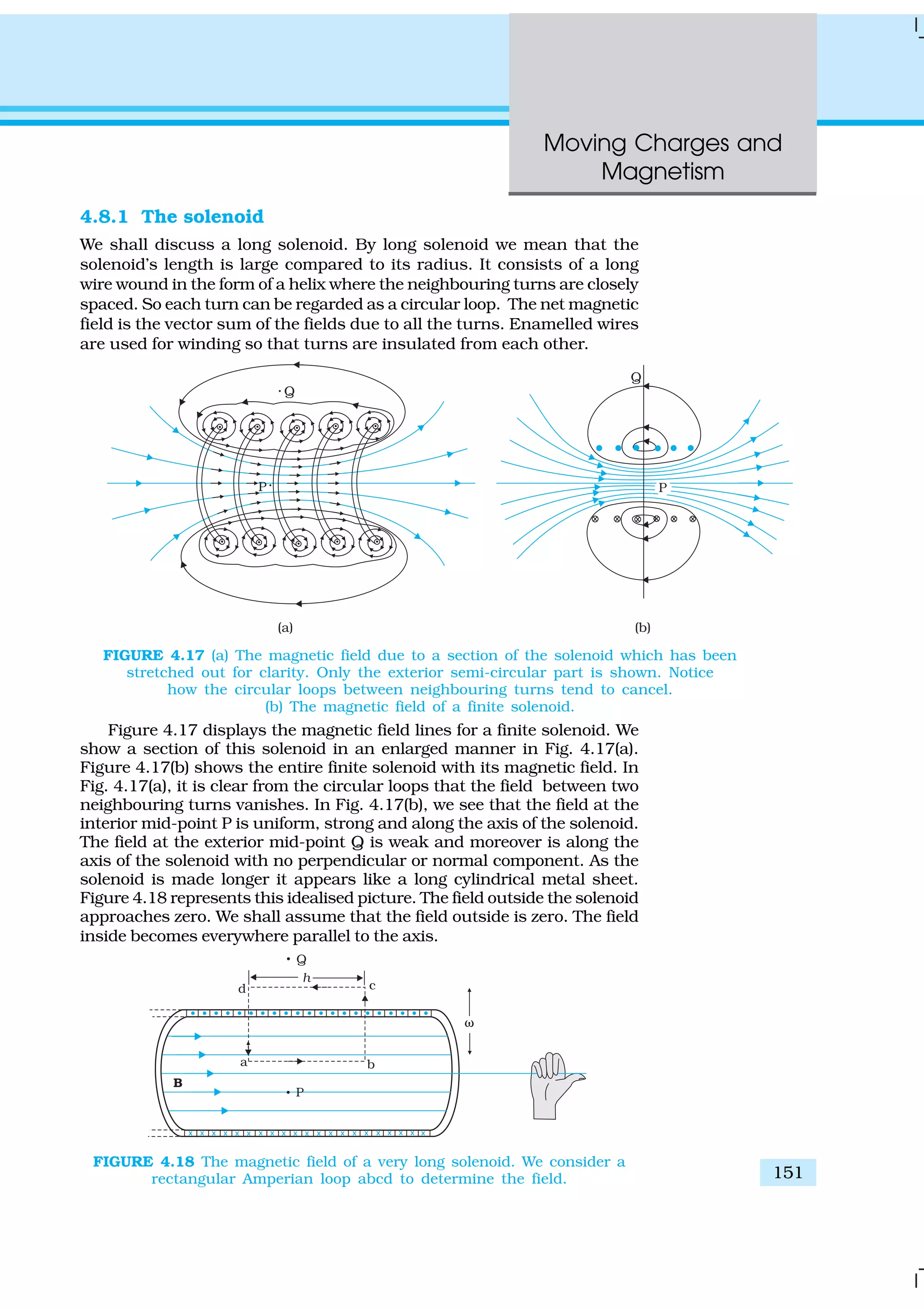
156. Physics
152
Consider a rectangular Amperian loop abcd. Along cd the field is zero
as argued above. Along transverse sections bc and ad, the field component
is zero. Thus, these two sections make no contribution. Let the field along
ab be B. Thus, the relevant length of the Amperian loop is, L = h.
Let n be the number of turns per unit length, then the total number
of turns is nh. The enclosed current is, Ie
= I (n h), where I is the current
in the solenoid. From Ampere’s circuital law [Eq. 4.17 (b)]
BL = µ0
Ie
, B h = µ0
I (n h)
B = µ0
n I (4.20)
The direction of the field is given by the right-hand rule. The solenoid
is commonly used to obtain a uniform magnetic field. We shall see in the
next chapter that a large field is possible by inserting a soft
iron core inside the solenoid.
4.8.2 The toroid
The toroid is a hollow circular ring on which a large number
of turns of a wire are closely wound. It can be viewed as a
solenoid which has been bent into a circular shape to close
on itself. It is shown in Fig. 4.19(a) carrying a current I. We
shall see that the magnetic field in the open space inside
(point P) and exterior to the toroid (point Q) is zero. The
field B inside the toroid is constant in magnitude for the
ideal toroid of closely wound turns.
Figure 4.19(b) shows a sectional view of the toroid. The
direction of the magnetic field inside is clockwise as per the
right-hand thumb rule for circular loops. Three circular
Amperian loops 1, 2 and 3 are shown by dashed lines. By
symmetry, the magnetic field should be tangential to each
of them and constant in magnitude for a given loop. The
circular areas bounded by loops 2 and 3 both cut the toroid:
so that each turn of current carrying wire is cut once by
the loop 2 and twice by the loop 3.
Let the magnetic field along loop 1 be B1
in magnitude.
Then in Ampere’s circuital law [Eq. 4.17(a)], L = 2π r1
.
However, the loop encloses no current, so Ie
= 0. Thus,
B1
(2 π r1
) = µ0
(0), B1
= 0
Thus, the magnetic field at any point P in the open space
inside the toroid is zero.
We shall now show that magnetic field at Q is likewise
zero. Let the magnetic field along loop 3 be B3
. Once again
from Ampere’s law L = 2 π r3
. However, from the sectional
cut, we see that the current coming out of the plane of the
paper is cancelled exactly by the current going into it. Thus,
Ie
= 0, and B3
= 0. Let the magnetic field inside the solenoid
be B. We shall now consider the magnetic field at S. Once again we employ
Ampere’s law in the form of Eq. [4.17 (a)]. We find, L = 2π r.
The current enclosed Ie
is (for N turns of toroidal coil) N I.
B (2πr) = µ0
NI
FIGURE 4.19 (a) A toroid carrying
a current I. (b) A sectional view of
the toroid. The magnetic field can
be obtained at an arbitrary
distance r from the centre O of
the toroid by Ampere’s circuital
law. The dashed lines labelled
1, 2 and 3 are three circular
Amperian loops.

157. Moving Charges and
Magnetism
153
0
2
NI
B
r
µ
=
π
(4.21)
We shall now compare the two results: for a toroid and solenoid. We
re-express Eq. (4.21) to make the comparison easier with the solenoid
result given in Eq. (4.20). Let r be the average radius of the toroid and n
be the number of turns per unit length. Then
N = 2πr n = (average) perimeter of the toroid
× number of turns per unit length
and thus,
B = µ0
n I, (4.22)
i.e., the result for the solenoid!
In an ideal toroid the coils are circular. In reality the turns of the
toroidal coil form a helix and there is always a small magnetic field external
to the toroid.
MAGNETIC CONFINEMENT
We have seen in Section 4.3 (see also the box on helical motion of charged particles earlier
in this chapter) that orbits of charged particles are helical. If the magnetic field is
non-uniform, but does not change much during one circular orbit, then the radius of the
helix will decrease as it enters stronger magnetic field and the radius will increase when it
enters weaker magnetic fields. We consider two solenoids at a distance from each other,
enclosed in an evacuated container (see figure below where we have not shown the container).
Charged particles moving in the region between the two solenoids will start with a small
radius. The radius will increase as field decreases and the radius will decrease again as
field due to the second solenoid takes over. The solenoids act as a mirror or reflector. [See
the direction of F as the particle approaches coil 2 in the figure. It has a horizontal component
against the forward motion.] This makes the particles turn back when they approach the
solenoid. Such an arrangement will act like magnetic bottle or magnetic container. The
particles will never touch the sides of the container. Such magnetic bottles are of great use
in confining the high energy plasma in fusion experiments. The plasma will destroy any
other form of material container because of it’s high temperature. Another useful container
is a toroid. Toroids are expected to play a key role in the tokamak, an equipment for plasma
confinement in fusion power reactors. There is an international collaboration called the
International Thermonuclear Experimental Reactor (ITER), being set up in France, for
achieving controlled fusion, of which India is a collaborating nation. For details of ITER
collaboration and the project, you may visit http://www.iter.org.

158. Physics
154
EXAMPLE4.9
Example 4.9 A solenoid of length 0.5 m has a radius of 1 cm and is
made up of 500 turns. It carries a current of 5 A. What is the
magnitude of the magnetic field inside the solenoid?
Solution The number of turns per unit length is,
500
1000
0.5
n = = turns/m
The length l = 0.5 m and radius r = 0.01 m. Thus, l/a = 50 i.e., l >> a.
Hence, we can use the long solenoid formula, namely, Eq. (4.20)
B = µ0
n I
= 4π × 10–7
× 103
× 5
= 6.28 × 10–3
T
4.9 FORCE BETWEEN TWO PARALLEL CURRENTS,
THE AMPERE
We have learnt that there exists a magnetic field due to a conductor
carrying a current which obeys the Biot-Savart law. Further, we have
learnt that an external magnetic field will exert a force on
a current-carrying conductor. This follows from the
Lorentz force formula. Thus, it is logical to expect that
two current-carrying conductors placed near each other
will exert (magnetic) forces on each other. In the period
1820-25, Ampere studied the nature of this magnetic
force and its dependence on the magnitude of the current,
on the shape and size of the conductors as well as the
distances between the conductors. In this section, we
shall take the simple example of two parallel current-
carrying conductors, which will perhaps help us to
appreciate Ampere’s painstaking work.
Figure 4.20 shows two long parallel conductors a
and b separated by a distance d and carrying (parallel)
currents Ia
and Ib
, respectively. The conductor ‘a’
produces, the same magnetic field Ba
at all points along
the conductor ‘b’. The right-hand rule tells us that the
direction of this field is downwards (when the conductors
are placed horizontally). Its magnitude is given by Eq. [4.19(a)] or from
Ampere’s circuital law,
0
2
a
a
I
B
d
µ
=
π
The conductor ‘b’ carrying a current Ib
will experience a sideways
force due to the field Ba
. The direction of this force is towards the
conductor ‘a’ (Verify this). We label this force as Fba
, the force on a
segment L of ‘b’ due to ‘a’. The magnitude of this force is given by
Eq. (4.4),
FIGURE 4.20 Two long straight
parallel conductors carrying steady
currents Ia
and Ib
and separated by a
distance d. Ba
is the magnetic field set
up by conductor ‘a’ at conductor ‘b’.

159. Moving Charges and
Magnetism
155
Fba
= Ib
L Ba
0
2
a bI I
L
d
µ
=
π (4.23)
It is of course possible to compute the force on ‘a’ due to ‘b’. From
considerations similar to above we can find the force Fab
, on a segment of
length L of ‘a’ due to the current in ‘b’. It is equal in magnitude to Fba
,
and directed towards ‘b’. Thus,
Fba
= –Fab
(4.24)
Note that this is consistent with Newton’s third Law. Thus, at least for
parallel conductors and steady currents, we have shown that the
Biot-Savart law and the Lorentz force yield results in accordance with
Newton’s third Law*.
We have seen from above that currents flowing in the same direction
attract each other. One can show that oppositely directed currents repel
each other. Thus,
Parallel currents attract, and antiparallel currents repel.
This rule is the opposite of what we find in electrostatics. Like (same
sign) charges repel each other, but like (parallel) currents attract each
other.
Let fba
represent the magnitude of the force Fba
per unit length. Then,
from Eq. (4.23),
ð
0
2
a b
ba
I I
f
d
µ
= (4.25)
The above expression is used to define the ampere (A), which is one
of the seven SI base units.
The ampere is the value of that steady current which, when maintained
in each of the two very long, straight, parallel conductors of negligible
cross-section, and placed one metre apart in vacuum, would produce
on each of these conductors a force equal to 2 × 10–7
newtons per metre
of length.
This definition of the ampere was adopted in 1946. It is a theoretical
definition. In practice one must eliminate the effect of the earth’s magnetic
field and substitute very long wires by multiturn coils of appropriate
geometries. An instrument called the current balance is used to measure
this mechanical force.
The SI unit of charge, namely, the coulomb, can now be defined in
terms of the ampere.
When a steady current of 1A is set up in a conductor, the quantity of
charge that flows through its cross-section in 1s is one coulomb (1C).
* It turns out that when we have time-dependent currents and/or charges in
motion, Newton’s third law may not hold for forces between charges and/or
conductors. An essential consequence of the Newton’s third law in mechanics
is conservation of momentum of an isolated system. This, however, holds even
for the case of time-dependent situations with electromagnetic fields, provided
the momentum carried by fields is also taken into account.

160. Physics
156
EXAMPLE4.10
Example 4.10 The horizontal component of the earth’s magnetic field
at a certain place is 3.0 ×10–5
T and the direction of the field is from
the geographic south to the geographic north. A very long straight
conductor is carrying a steady current of 1A. What is the force per
unit length on it when it is placed on a horizontal table and the
direction of the current is (a) east to west; (b) south to north?
Solution F = Il × B
F = IlB sinθ
The force per unit length is
f = F/l = I B sinθ
(a) When the current is flowing from east to west,
θ = 90°
Hence,
f = I B
= 1 × 3 × 10–5
= 3 × 10–5
N m–1
ROGET’S SPIRAL FOR ATTRACTION BETWEEN PARALLEL CURRENTS
Magnetic effects are generally smaller than electric effects. As a consequence, the force
between currents is rather small, because of the smallness of the factor µ. Hence it is
difficult to demonstrate attraction or repulsion between currents. Thus for 5 A current
in each wire at a separation of 1cm, the force per metre would be 5 × 10–4
N, which is
about 50 mg weight. It would be like pulling a wire by a string going over a pulley to
which a 50 mg weight is attached. The displacement of the wire would be quite
unnoticeable.
With the use of a soft spring, we can increase the effective length of the parallel current
and by using mercury, we can make the displacement of even a few mm observable very
dramatically. You will also need a constant-current
supply giving a constant current of about 5 A.
Take a soft spring whose natural period of
oscillations is about 0.5 – 1s. Hang it vertically and
attach a pointed tip to its lower end, as shown in the
figure here. Take some mercury in a dish and adjust the
spring such that the tip is just above the mercury
surface. Take the DC current source, connect one of its
terminals to the upper end of the spring, and dip the
other terminal in mercury. If the tip of the spring touches
mercury, the circuit is completed through mercury.
Let the DC source be put off to begin with. Let the tip be adjusted so that it just
touches the mercury surface. Switch on the constant current supply, and watch the
fascinating outcome. The spring shrinks with a jerk, the tip comes out of mercury (just
by a mm or so), the circuit is broken, the current stops, the spring relaxes and tries to
come back to its original position, the tip again touches mercury establishing a current
in the circuit, and the cycle continues with tick, tick, tick, . . . . In the beginning, you
may require some small adjustments to get a good effect.
Keep your face away from mercury vapours as they are poisonous. Do not inhale
mercury vapours for long.

161. Moving Charges and
Magnetism
157
EXAMPLE4.10
This is larger than the value 2×10–7
Nm–1
quoted in the definition
of the ampere. Hence it is important to eliminate the effect of the
earth’s magnetic field and other stray fields while standardising
the ampere.
The direction of the force is downwards. This direction may be
obtained by the directional property of cross product of vectors.
(b) When the current is flowing from south to north,
θ = 0o
f = 0
Hence there is no force on the conductor.
4.10 TORQUE ON CURRENT LOOP, MAGNETIC DIPOLE
4.10.1 Torque on a rectangular current loop in a uniform
magnetic field
We now show that a rectangular loop carrying a steady current I and
placed in a uniform magnetic field experiences a torque. It does not
experience a net force. This behaviour is analogous to
that of electric dipole in a uniform electric field
(Section 1.10).
We first consider the simple case when the
rectangular loop is placed such that the uniform
magnetic field B is in the plane of the loop. This is
illustrated in Fig. 4.21(a).
The field exerts no force on the two arms AD and BC
of the loop. It is perpendicular to the arm AB of the loop
and exerts a force F1
on it which is directed into the
plane of the loop. Its magnitude is,
F1
= I b B
Similarly it exerts a force F2
on the arm CD and F2
is directed out of the plane of the paper.
F2
= I b B = F1
Thus, the net force on the loop is zero. There is a
torque on the loop due to the pair of forces F1
and F2
.
Figure 4.21(b) shows a view of the loop from the AD
end. It shows that the torque on the loop tends to rotate
it anti-clockwise. This torque is (in magnitude),
1 2
2 2
a a
F Fτ = +
( )
2 2
a a
IbB IbB I ab B= + =
= I A B (4.26)
where A = ab is the area of the rectangle.
We next consider the case when the plane of the loop,
is not along the magnetic field, but makes an angle with
it. We take the angle between the field and the normal to
FIGURE 4.21 (a) A rectangular
current-carrying coil in uniform
magnetic field. The magnetic moment
m points downwards. The torque τ is
along the axis and tends to rotate the
coil anticlockwise. (b) The couple
acting on the coil.

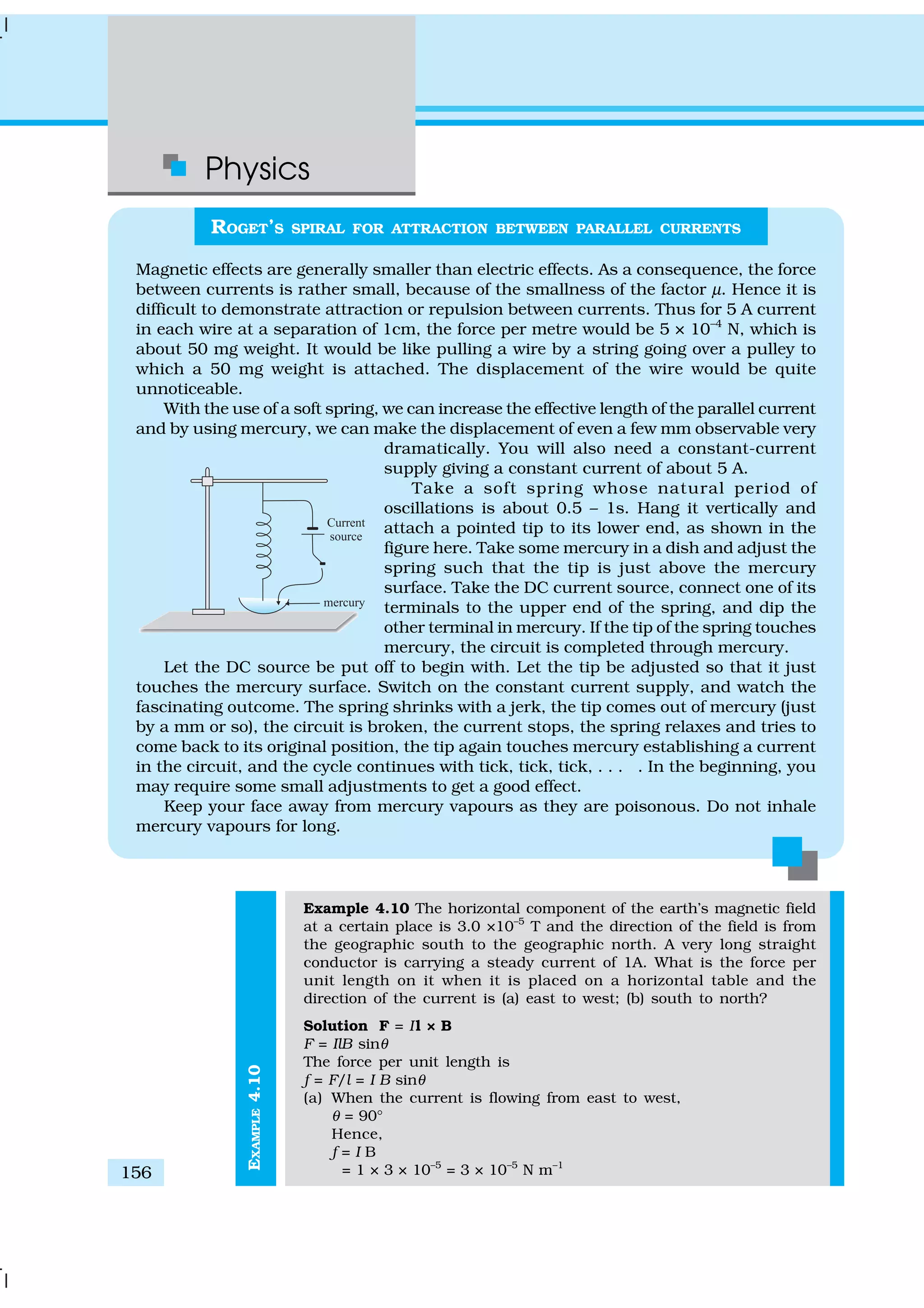
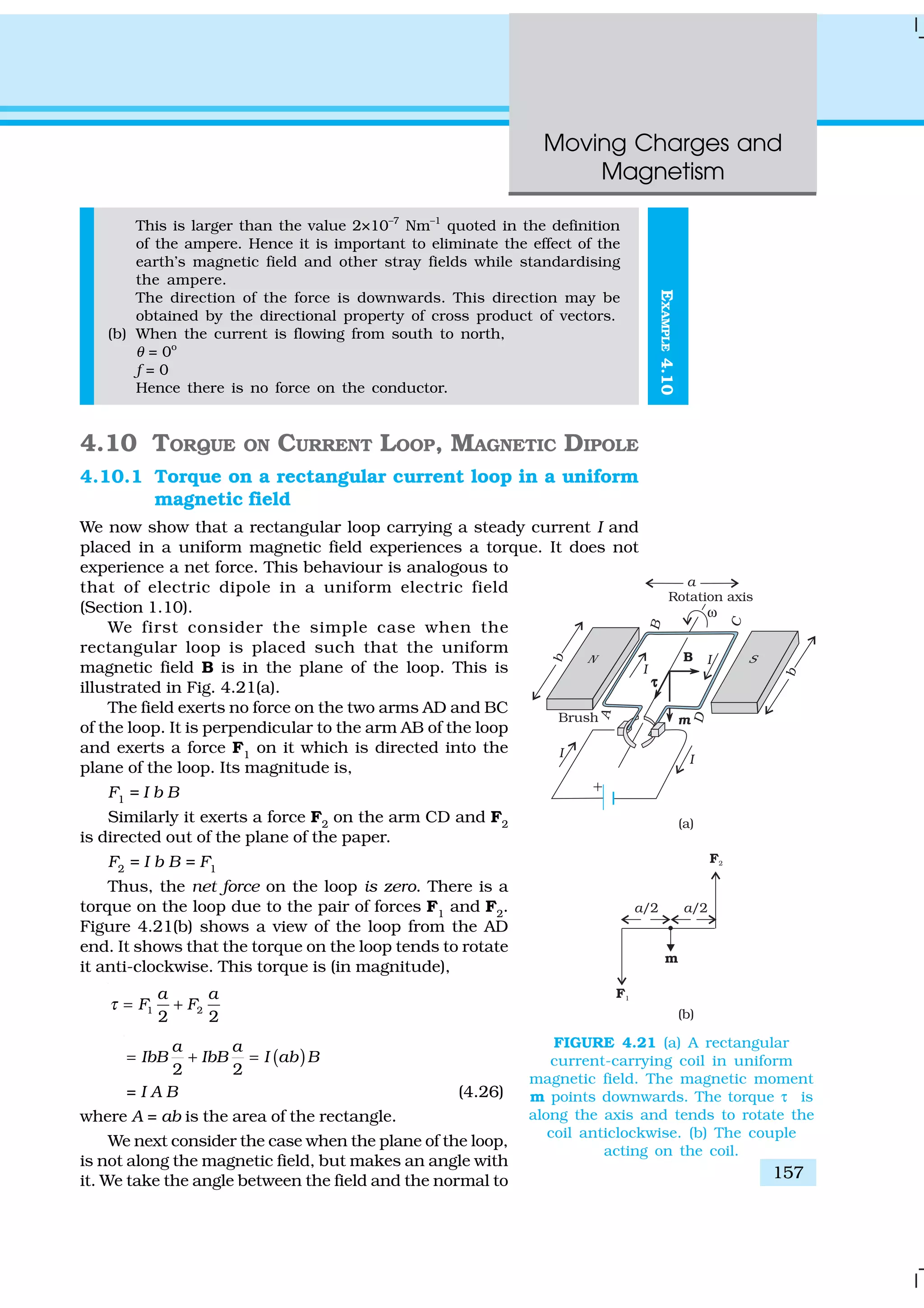
162. Physics
158
the coil to be angle θ (The previous case
corresponds to θ = π/2). Figure 4.22 illustrates
this general case.
The forces on the arms BC and DA are equal,
opposite, and act along the axis of the coil, which
connects the centres of mass of BC and DA. Being
collinear along the axis they cancel each other,
resulting in no net force or torque. The forces on
arms AB and CD are F1
and F2
. They too are equal
and opposite, with magnitude,
F1
= F2
= I b B
But they are not collinear! This results in a
couple as before. The torque is, however, less than
the earlier case when plane of loop was along the
magnetic field. This is because the perpendicular
distance between the forces of the couple has
decreased. Figure 4.22(b) is a view of the
arrangement from the AD end and it illustrates
these two forces constituting a couple. The
magnitude of the torque on the loop is,
1 2sin sin
2 2
a a
F Fτ θ θ= +
= I ab B sin θ
= I A B sin θ (4.27)
As θ à 0, the perpendicular distance between
the forces of the couple also approaches zero. This
makes the forces collinear and the net force and
torque zero. The torques in Eqs. (4.26) and (4.27)
can be expressed as vector product of the magnetic moment of the coil
and the magnetic field. We define the magnetic moment of the current
loop as,
m = I A (4.28)
where the direction of the area vector A is given by the right-hand thumb
rule and is directed into the plane of the paper in Fig. 4.21. Then as the
angle between m and B is θ , Eqs. (4.26) and (4.27) can be expressed by
one expression
= ×m Bτ (4.29)
This is analogous to the electrostatic case (Electric dipole of dipole
moment pe
in an electric field E).
e= ×p Eτ
As is clear from Eq. (4.28), the dimensions of the magnetic moment are
[A][L2
] and its unit is Am2
.
From Eq. (4.29), we see that the torque ττ vanishes when m is either
parallel or antiparallel to the magnetic field B. This indicates a state of
equilibrium as there is no torque on the coil (this also applies to any
object with a magnetic moment m). When m and B are parallel the
FIGURE 4.22 (a) The area vector of the loop
ABCD makes an arbitrary angle θ with
the magnetic field. (b) Top view of
the loop. The forces F1
and F2
acting
on the arms AB and CD
are indicated.

163. Moving Charges and
Magnetism
159
EXAMPLE4.11
equilibrium is a stable one. Any small rotation of the coil produces a
torque which brings it back to its original position. When they are
antiparallel, the equilibrium is unstable as any rotation produces a torque
which increases with the amount of rotation. The presence of this torque
is also the reason why a small magnet or any magnetic dipole aligns
itself with the external magnetic field.
If the loop has N closely wound turns, the expression for torque, Eq.
(4.29), still holds, with
m = N I A (4.30)
Example 4.11 A 100 turn closely wound circular coil of radius 10 cm
carries a current of 3.2 A. (a) What is the field at the centre of the
coil? (b) What is the magnetic moment of this coil?
The coil is placed in a vertical plane and is free to rotate about a
horizontal axis which coincides with its diameter. A uniform magnetic
field of 2T in the horizontal direction exists such that initially the
axis of the coil is in the direction of the field. The coil rotates through
an angle of 90º under the influence of the magnetic field.
(c) What are the magnitudes of the torques on the coil in the initial
and final position? (d) What is the angular speed acquired by the
coil when it has rotated by 90º? The moment of inertia of the coil is
0.1 kg m2
.
Solution
(a) From Eq. (4.16)
0
2
NI
B
R
µ
=
Here, N = 100; I = 3.2 A, and R = 0.1 m. Hence,
7 2
1
4 10 10 3.2
2 10
B
−
−
π × × ×
=
×
5
1
4 10 10
2 10
−
−
× ×
=
×
(using π × 3.2 = 10)
= 2 × 10–3
T
The direction is given by the right-hand thumb rule.
(b) The magnetic moment is given by Eq. (4.30),
m = N I A = N I π r2
= 100 × 3.2 × 3.14 × 10–2
= 10 A m2
The direction is once again given by the right hand thumb rule.
(c) τ = ×m B [from Eq. (4.29)]
sinm B θ=
Initially, θ = 0. Thus, initial torque τi
= 0. Finally, θ = π/2 (or 90º).
Thus, final torque τf
= m B = 10 × 2 = 20 N m.
(d) From Newton’s second law,
1
d
sin
d
m B
t
ω
θ=
where 1 is the moment of inertia of the coil. From chain rule,
d d d d
d d d dt t
ω ω θ ω
ω
θ θ
= =
Using this,
1 d sin dm Bω ω θ θ=

164. Physics
160
EXAMPLE4.12EXAMPLE4.11
Integrating from θ = 0 to θ = π/2,
ð / 2
0 0
d sin d
f
m B
ω
ω ω θ θ=∫ ∫1
2
/2
0
cos
2
f
m B
ω
θ
π
= −1 = m B
1/2
2
f
m B
ω
 
=   1
1/2
1
2 20
10−
× 
=   
= 20 s–1
.
Example 4.12
(a) A current-carrying circular loop lies on a smooth horizontal plane.
Can a uniform magnetic field be set up in such a manner that
the loop turns around itself (i.e., turns about the vertical axis).
(b) A current-carrying circular loop is located in a uniform external
magnetic field. If the loop is free to turn, what is its orientation
of stable equilibrium? Show that in this orientation, the flux of
the total field (external field + field produced by the loop) is
maximum.
(c) A loop of irregular shape carrying current is located in an external
magnetic field. If the wire is flexible, why does it change to a
circular shape?
Solution
(a) No, because that would require ττ to be in the vertical direction.
But ττ = I A × B, and since A of the horizontal loop is in the vertical
direction, τ would be in the plane of the loop for any B.
(b) Orientation of stable equilibrium is one where the area vector A
of the loop is in the direction of external magnetic field. In this
orientation, the magnetic field produced by the loop is in the same
direction as external field, both normal to the plane of the loop,
thus giving rise to maximum flux of the total field.
(c) It assumes circular shape with its plane normal to the field to
maximize flux, since for a given perimeter, a circle encloses greater
area than any other shape.
4.10.2 Circular current loop as a magnetic dipole
In this section, we shall consider the elementary magnetic element: the
current loop. We shall show that the magnetic field (at large distances)
due to current in a circular current loop is very similar in behavior to the
electric field of an electric dipole. In Section 4.6, we have evaluated the
magnetic field on the axis of a circular loop, of a radius R, carrying a
steady current I. The magnitude of this field is [(Eq. (4.15)],
( )
2
0
3/22 2
2
I R
B
x R
µ
=
+
and its direction is along the axis and given by the right-hand thumb
rule (Fig. 4.12). Here, x is the distance along the axis from the centre of
the loop. For x >> R, we may drop the R2
term in the denominator. Thus,

165. Moving Charges and
Magnetism
161
2
0
3
2
R
B
x
µ
=
Note that the area of the loop A = πR2
. Thus,
0
3
2
IA
B
x
µ
=
π
As earlier, we define the magnetic moment m to have a magnitude IA,
m = I A. Hence,
ð
0
3
2 x
µ m
B ;
ð
0
3
2
4 x
µ
=
m
[4.31(a)]
The expression of Eq. [4.31(a)] is very similar to an expression obtained
earlier for the electric field of a dipole. The similarity may be seen if we
substitute,
0 01/µ ε→
e→m p (electrostatic dipole)
→B E (electrostatic field)
We then obtain,
3
0
2
4
e
xε
=
π
p
E
which is precisely the field for an electric dipole at a point on its axis.
considered in Chapter 1, Section 1.10 [Eq. (1.20)].
It can be shown that the above analogy can be carried further. We
had found in Chapter 1 that the electric field on the perpendicular bisector
of the dipole is given by [See Eq.(1.21)],
3
04
e
xεπ
p
E ;
where x is the distance from the dipole. If we replace p à m and 0 01/µ ε→
in the above expression, we obtain the result for B for a point in the
plane of the loop at a distance x from the centre. For x >>R,
0
3
;
4
x R
x
µ
>>
π
m
B ; [4.31(b)]
The results given by Eqs. [4.31(a)] and [4.31(b)] become exact for a
point magnetic dipole.
The results obtained above can be shown to apply to any planar loop:
a planar current loop is equivalent to a magnetic dipole of dipole moment
m = I A, which is the analogue of electric dipole moment p. Note, however,
a fundamental difference: an electric dipole is built up of two elementary
units — the charges (or electric monopoles). In magnetism, a magnetic
dipole (or a current loop) is the most elementary element. The equivalent
of electric charges, i.e., magnetic monopoles, are not known to exist.
We have shown that a current loop (i) produces a magnetic field (see
Fig. 4.12) and behaves like a magnetic dipole at large distances, and

166. Physics
162
(ii) is subject to torque like a magnetic needle. This led Ampere to suggest
that all magnetism is due to circulating currents. This seems to be partly
true and no magnetic monopoles have been seen so far. However,
elementary particles such as an electron or a proton also carry an intrinsic
magnetic moment, not accounted by circulating currents.
4.10.3 The magnetic dipole moment of a revolving electron
In Chapter 12 we shall read about the Bohr model of the hydrogen atom.
You may perhaps have heard of this model which was proposed by the
Danish physicist Niels Bohr in 1911 and was a stepping stone
to a new kind of mechanics, namely, quantum mechanics.
In the Bohr model, the electron (a negatively charged particle)
revolves around a positively charged nucleus much as a
planet revolves around the sun. The force in the former case
is electrostatic (Coulomb force) while it is gravitational for
the planet-Sun case. We show this Bohr picture of the electron
in Fig. 4.23.
The electron of charge (–e) (e = + 1.6 × 10–19
C) performs
uniform circular motion around a stationary heavy nucleus
of charge +Ze. This constitutes a current I, where,
e
I
T
= (4.32)
and T is the time period of revolution. Let r be the orbital
radius of the electron, and v the orbital speed. Then,
ð2 r
T =
v
(4.33)
Substituting in Eq. (4.32), we have I = ev/2πr.
There will be a magnetic moment, usually denoted by µl
,
associated with this circulating current. From Eq. (4.28) its
magnitude is, µl
= Iπr2
= evr/2.
The direction of this magnetic moment is into the plane
of the paper in Fig. 4.23. [This follows from the right-hand
rule discussed earlier and the fact that the negatively charged
electron is moving anti-clockwise, leading to a clockwise current.]
Multiplying and dividing the right-hand side of the above expression by
the electron mass me
, we have,
( )
2
l e
e
e
m vr
m
µ =
2 e
e
l
m
= [4.34(a)]
Here, l is the magnitude of the angular momentum of the electron
about the central nucleus (“orbital” angular momentum). Vectorially,
2
l
e
e
m
= − lµ [4.34(b)]
The negative sign indicates that the angular momentum of the electron
is opposite in direction to the magnetic moment. Instead of electron with
FIGURE 4.23 In the Bohr model
of hydrogen-like atoms, the
negatively charged electron is
revolving with uniform speed
around a centrally placed
positively charged (+Z e)
nucleus. The uniform circular
motion of the electron
constitutes a current. The
direction of the magnetic
moment is into the plane of the
paper and is indicated
separately by ⊗.

167. Moving Charges and
Magnetism
163
charge (–e), if we had taken a particle with charge (+q), the angular
momentum and magnetic moment would be in the same direction. The
ratio
l
2 e
e
l m
µ
= (4.35)
is called the gyromagnetic ratio and is a constant. Its value is 8.8 × 1010
C /kg
for an electron, which has been verified by experiments.
The fact that even at an atomic level there is a magnetic moment,
confirms Ampere’s bold hypothesis of atomic magnetic moments. This
according to Ampere, would help one to explain the magnetic properties
of materials. Can one assign a value to this atomic dipole moment? The
answer is Yes. One can do so within the Bohr model. Bohr hypothesised
that the angular momentum assumes a discrete set of values, namely,
2
n h
l =
π (4.36)
where n is a natural number, n = 1, 2, 3, .... and h is a constant named
after Max Planck (Planck’s constant) with a value h = 6.626 × 10–34
J s.
This condition of discreteness is called the Bohr quantisation condition.
We shall discuss it in detail in Chapter 12. Our aim here is merely to use
it to calculate the elementary dipole moment. Take the value n = 1, we
have from Eq. (4.34) that,
min( )
4
l
e
e
h
m
µ =
π
19 34
31
1.60 10 6.63 10
4 3.14 9.11 10
− −
−
× × ×
=
× × ×
= 9.27 × 10–24
Am2
(4.37)
where the subscript ‘min’ stands for minimum. This value is called the
Bohr magneton.
Any charge in uniform circular motion would have an associated
magnetic moment given by an expression similar to Eq. (4.34). This dipole
moment is labelled as the orbital magnetic moment. Hence the subscript
‘l’ in µl
. Besides the orbital moment, the electron has an intrinsic magnetic
moment, which has the same numerical value as given in Eq. (4.37). It is
called the spin magnetic moment. But we hasten to add that it is not as
though the electron is spinning. The electron is an elementary particle
and it does not have an axis to spin around like a top or our earth.
Nevertheless it does possess this intrinsic magnetic moment. The
microscopic roots of magnetism in iron and other materials can be traced
back to this intrinsic spin magnetic moment.
4.11 THE MOVING COIL GALVANOMETER
Currents and voltages in circuits have been discussed extensively in
Chapters 3. But how do we measure them? How do we claim that
current in a circuit is 1.5 A or the voltage drop across a resistor is 1.2 V?
Figure 4.24 exhibits a very useful instrument for this purpose: the moving
Conversionofgalvanometerintoameterandvoltmeter:
http://patsy.hunter.cuny.edu/CORE/CORE4/LectureNotes/Electricity/electric6.htm

168. Physics
164
coil galvanometer (MCG). It is a device whose principle can be understood
on the basis of our discussion in Section 4.10.
The galvanometer consists of a coil, with many turns, free to rotate
about a fixed axis (Fig. 4.24), in a uniform radial magnetic field. There is
a cylindrical soft iron core which not only makes the field radial but also
increases the strength of the magnetic field. When a current flows through
the coil, a torque acts on it. This torque is given by Eq. (4.26) to be
τ = NI AB
where the symbols have their usual meaning. Since the field is radial by
design, we have taken sin θ = 1 in the above expression for the torque.
The magnetic torque NIAB tends to rotate the coil. A spring Sp
provides a
counter torque kφ that balances the magnetic torque NIAB; resulting in a
steady angular deflection φ. In equilibrium
kφ = NI AB
where k is the torsional constant of the spring; i.e. the restoring torque
per unit twist. The deflection φ is indicated on the scale by a pointer
attached to the spring. We have
NAB
I
k
φ
 
=    (4.38)
The quantity in brackets is a constant for a given
galvanometer.
The galvanometer can be used in a number of ways.
It can be used as a detector to check if a current is
flowing in the circuit. We have come across this usage
in the Wheatstone’s bridge arrangement. In this usage
the neutral position of the pointer (when no current is
flowing through the galvanometer) is in the middle of
the scale and not at the left end as shown in Fig.4.24.
Depending on the direction of the current, the pointer
deflection is either to the right or the left.
The galvanometer cannot as such be used as an
ammeter to measure the value of the current in a given
circuit. This is for two reasons: (i) Galvanometer is a
very sensitive device, it gives a full-scale deflection for
a current of the order of µA. (ii) For measuring
currents, the galvanometer has to be connected in
series, and as it has a large resistance, this will change
the value of the current in the circuit. To overcome
these difficulties, one attaches a small resistance rs
,
called shunt resistance, in parallel with
the galvanometer coil; so that most of the current
passes through the shunt. The resistance of this
arrangement is,
RG
rs
/ (RG
+ rs
) ; rs
if RG
>> rs
If rs
has small value, in relation to the resistance of
the rest of the circuit Rc
, the effect of introducing the
measuring instrument is also small and negligible. This
FIGURE 4.24 The moving coil
galvanometer. Its elements are
described in the text. Depending on
the requirement, this device can be
used as a current detector or for
measuring the value of the current
(ammeter) or voltage (voltmeter).

169. Moving Charges and
Magnetism
165
arrangement is schematically shown in Fig. 4.25. The scale of this
ammeter is calibrated and then graduated to read off the current value
with ease. We define the current sensitivity of the galvanometer as the
deflection per unit current. From Eq. (4.38) this current sensitivity is,
NAB
I k
φ
= (4.39)
A convenient way for the manufacturer to increase the sensitivity is
to increase the number of turns N. We choose galvanometers having
sensitivities of value, required by our experiment.
The galvanometer can also be used as a voltmeter to measure the
voltage across a given section of the circuit. For this it must be connected
in parallel with that section of the circuit. Further, it must draw a very
small current, otherwise the voltage measurement will disturb the original
set up by an amount which is very large. Usually we like to keep the
disturbance due to the measuring device below one per cent. To ensure
this, a large resistance R is connected in series with the galvanometer.
This arrangement is schematically depicted in Fig.4.26. Note that the
resistance of the voltmeter is now,
RG
+ R ; R : large
The scale of the voltmeter is calibrated to read off the voltage value
with ease. We define the voltage sensitivity as the deflection per unit
voltage. From Eq. (4.38),
1NAB I NAB
V k V k R
φ    
= =       (4.40)
An interesting point to note is that increasing the current sensitivity
may not necessarily increase the voltage sensitivity. Let us take Eq. (4.39)
which provides a measure of current sensitivity. If N → 2N, i.e., we double
the number of turns, then
2
I I
φ φ
→
Thus, the current sensitivity doubles. However, the resistance of the
galvanometer is also likely to double, since it is proportional to the length
of the wire. In Eq. (4.40), N →2N, and R →2R, thus the voltage sensitivity,
V V
φ φ
→
remains unchanged. So in general, the modification needed for conversion
of a galvanometer to an ammeter will be different from what is needed
for converting it into a voltmeter.
Example 4.13 In the circuit (Fig. 4.27) the current is to be
measured. What is the value of the current if the ammeter shown
(a) is a galvanometer with a resistance RG
= 60.00 Ω; (b) is a
galvanometer described in (a) but converted to an ammeter by a
shunt resistance rs
= 0.02 Ω; (c) is an ideal ammeter with zero
resistance?
FIGURE 4.25
Conversion of a
galvanometer (G) to
an ammeter by the
introduction of a
shunt resistance rs
of
very small value in
parallel.
FIGURE 4.26
Conversion of a
galvanometer (G) to a
voltmeter by the
introduction of a
resistance R of large
value in series.
EXAMPLE4.13

170. Physics
166
FIGURE 4.27
Solution
(a) Total resistance in the circuit is,
3 63GR + = Ω . Hence, I = 3/63 = 0.048 A.
(b) Resistance of the galvanometer converted to an ammeter is,
60 0.02
- 0.02
(60 0.02)
G s
G s
R r
R r
Ω × Ω
= Ω
+ + Ω
%
Total resistance in the circuit is,
0.02 3 3.02Ω + Ω = Ω . Hence, I = 3/3.02 = 0.99 A.
(c) For the ideal ammeter with zero resistance,
I = 3/3 = 1.00 A
SUMMARY
1. The total force on a charge q moving with velocity v in the presence of
magnetic and electric fields B and E, respectively is called the Lorentz
force. It is given by the expression:
F = q (v × B + E)
The magnetic force q (v × B) is normal to v and work done by it is zero.
2. A straight conductor of length l and carrying a steady current I
experiences a force F in a uniform external magnetic field B,
F = I l × B
where|l| = l and the direction of l is given by the direction of the
current.
3. In a uniform magnetic field B, a charge q executes a circular orbit in
a plane normal to B. Its frequency of uniform circular motion is called
the cyclotron frequency and is given by:
2
c
q B
m
ν =
π
This frequency is independent of the particle’s speed and radius. This
fact is exploited in a machine, the cyclotron, which is used to
accelerate charged particles.
4. The Biot-Savart law asserts that the magnetic field dB due to an
element dl carrying a steady current I at a point P at a distance r from
the current element is:
0
3
d
d
4
I
r
µ ×
=
π
l r
B
EXAMPLE4.13

171. Moving Charges and
Magnetism
167
To obtain the total field at P, we must integrate this vector expression
over the entire length of the conductor.
5. The magnitude of the magnetic field due to a circular coil of radius R
carrying a current I at an axial distance x from the centre is
2
0
2 2 3/2
2( )
IR
B
x R
µ
=
+
At the center this reduces to
0
2
I
B
R
µ
=
6. Ampere’s Circuital Law: Let an open surface S be bounded by a loop
C. Then the Ampere’s law states that 0
C
d Iµ=∫ B lgÑ where I refers to
the current passing through S. The sign of I is determined from the
right-hand rule. We have discussed a simplified form of this law. If B
is directed along the tangent to every point on the perimeter L of a
closed curve and is constant in magnitude along perimeter then,
BL = µ0
Ie
where Ie
is the net current enclosed by the closed circuit.
7. The magnitude of the magnetic field at a distance R from a long,
straight wire carrying a current I is given by:
ð
0
2
I
B
R
µ
=
The field lines are circles concentric with the wire.
8. The magnitude of the field B inside a long solenoid carrying a current
I is
B = µ0
nI
where n is the number of turns per unit length. For a toroid one
obtains,
0
2
NI
B
r
µ
=
π
where N is the total number of turns and r is the average radius.
9. Parallel currents attract and anti-parallel currents repel.
10. A planar loop carrying a current I, having N closely wound turns, and
an area A possesses a magnetic moment m where,
m = N I A
and the direction of m is given by the right-hand thumb rule : curl
the palm of your right hand along the loop with the fingers pointing
in the direction of the current. The thumb sticking out gives the
direction of m (and A)
When this loop is placed in a uniform magnetic field B, the force F on
it is: F = 0
And the torque on it is,
ττ = m × B
In a moving coil galvanometer, this torque is balanced by a counter-
torque due to a spring, yielding
kφ = NI AB

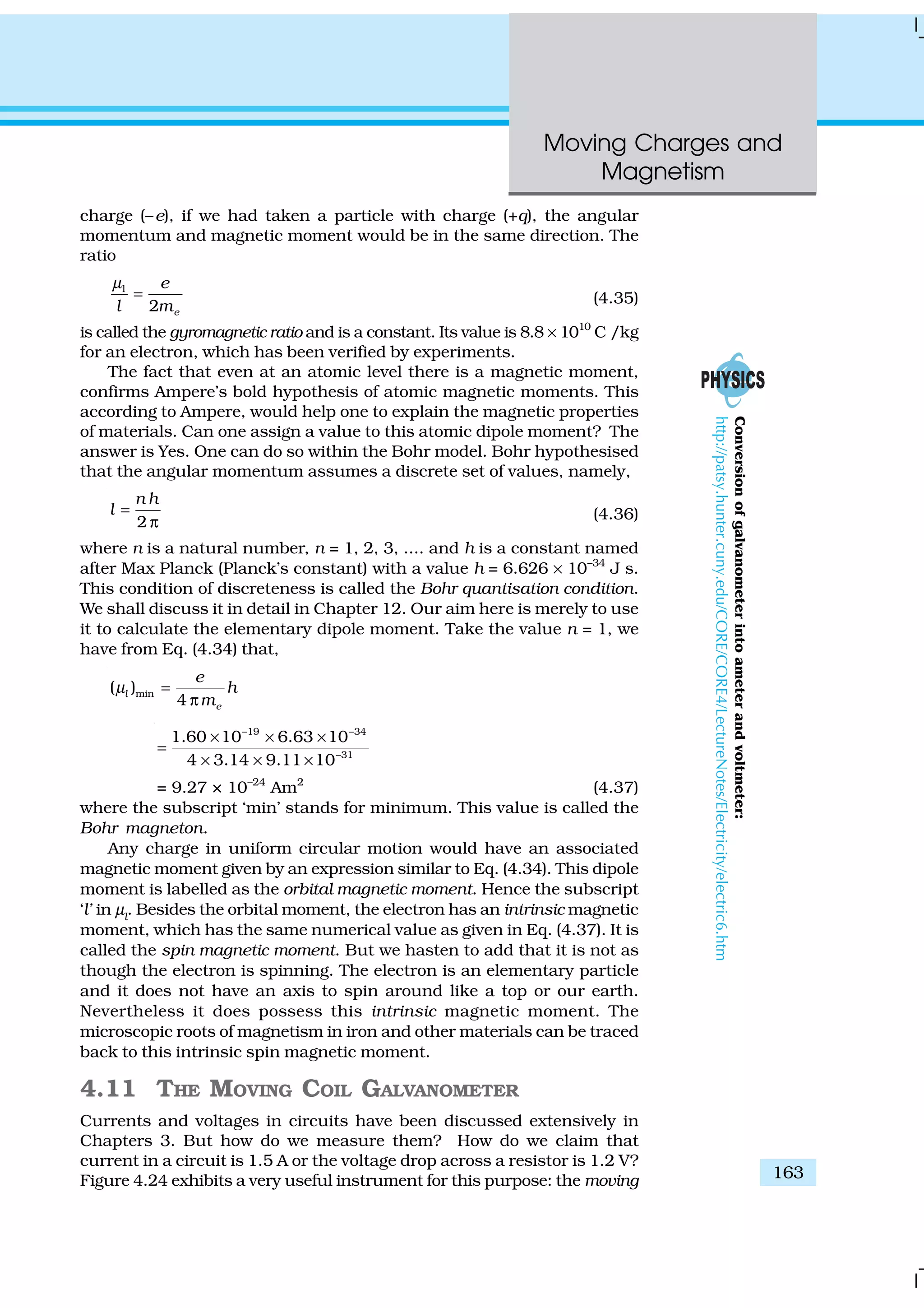
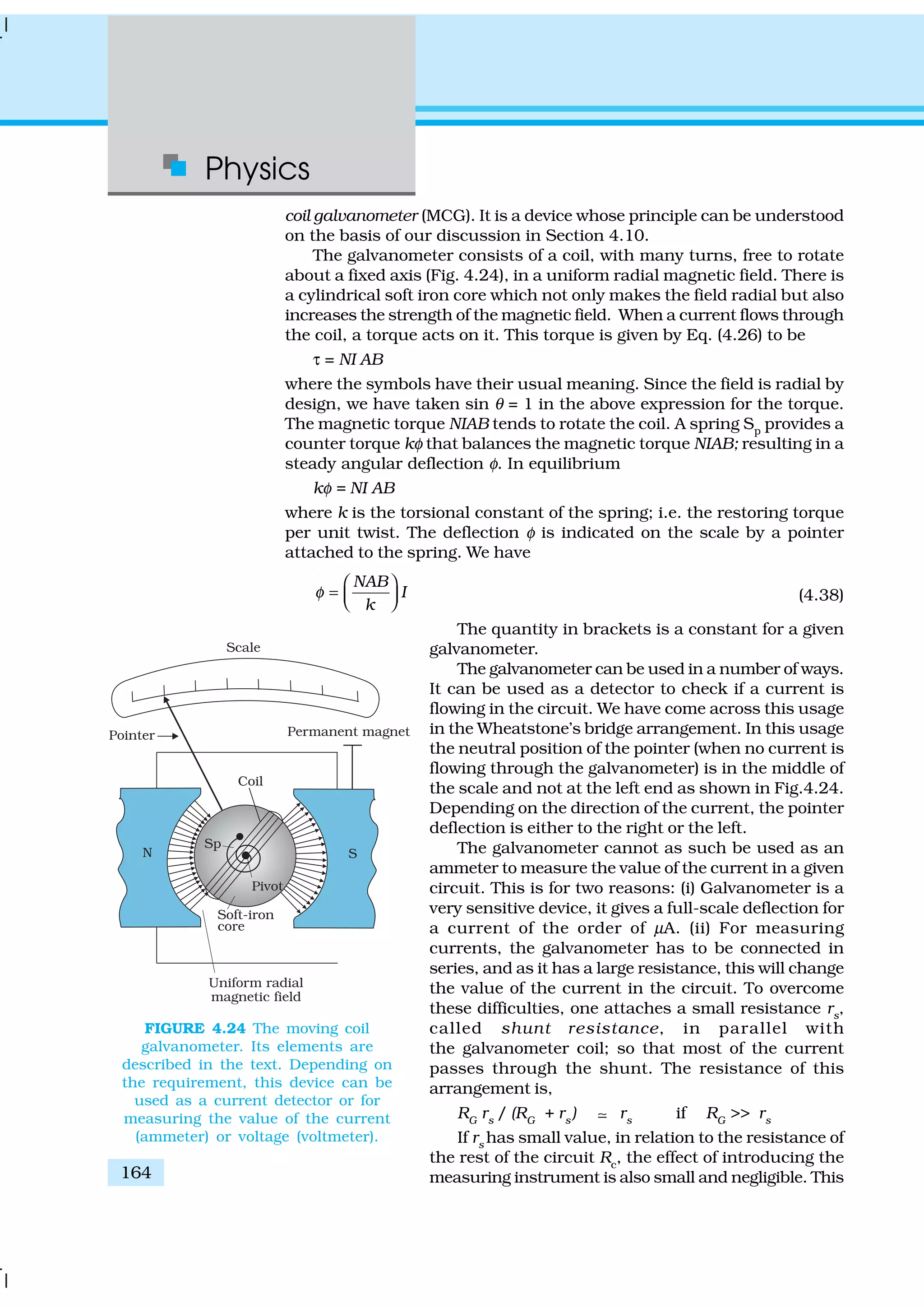
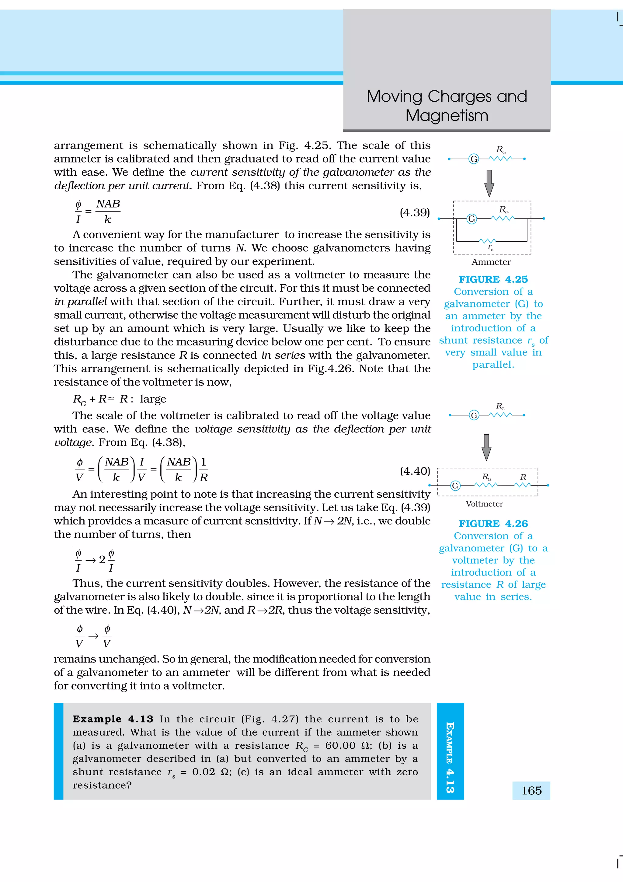
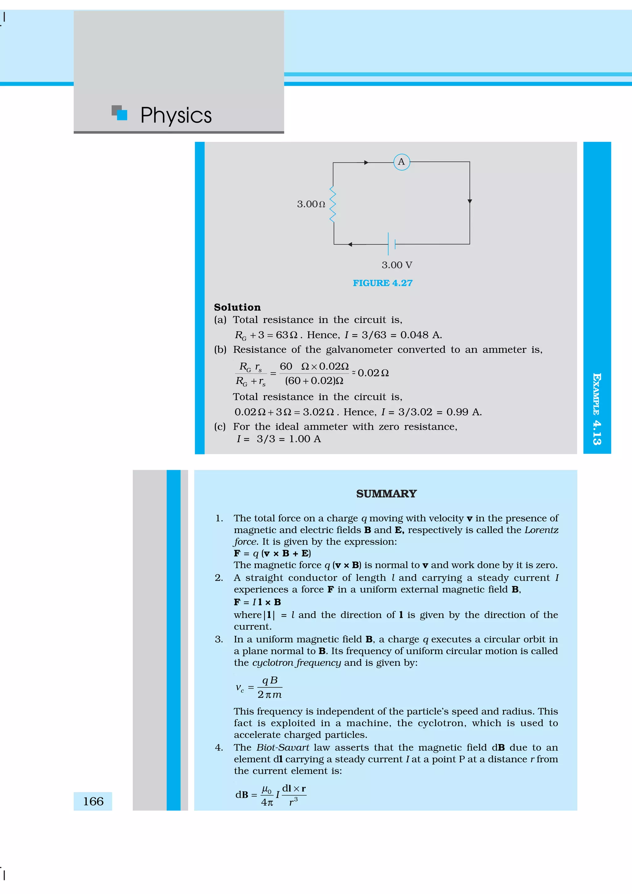
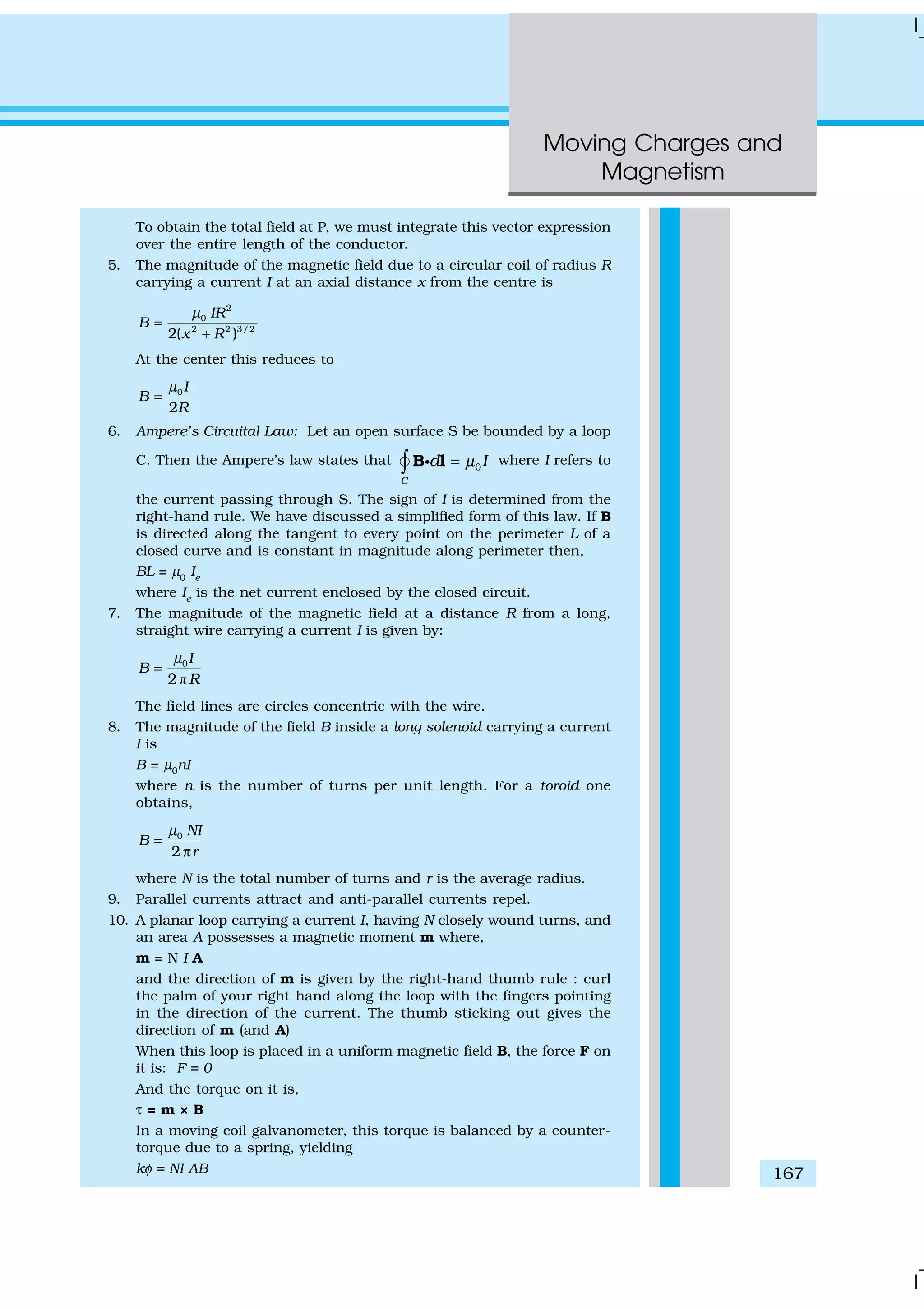
172. Physics
168
where φ is the equilibrium deflection and k the torsion constant of
the spring.
11. An electron moving around the central nucleus has a magnetic moment
µl
given by:
2
l
e
l
m
µ =
where l is the magnitude of the angular momentum of the circulating
electron about the central nucleus. The smallest value of µl
is called
the Bohr magneton µB
and it is µB
= 9.27×10–24
J/T
12. A moving coil galvanometer can be converted into a ammeter by
introducing a shunt resistance rs
, of small value in parallel. It can be
converted into a voltmeter by introducing a resistance of a large value
in series.
Physical Quantity Symbol Nature Dimensions Units Remarks
Permeability of free µ0
Scalar [MLT–2
A–2
] T m A–1
4π × 10–7
T m A–1
space
Magnetic Field B Vector [M T–2
A–1
] T (telsa)
Magnetic Moment m Vector [L2
A] A m2
or J/T
Torsion Constant k Scalar [M L2
T–2
] N m rad–1
Appears in MCG
POINTS TO PONDER
1. Electrostatic field lines originate at a positive charge and terminate at a
negative charge or fade at infinity. Magnetic field lines always form
closed loops.
2. The discussion in this Chapter holds only for steady currents which do
not vary with time.
When currents vary with time Newton’s third law is valid only if momentum
carried by the electromagnetic field is taken into account.
3. Recall the expression for the Lorentz force,
F = q (v × B + E)
This velocity dependent force has occupied the attention of some of the
greatest scientific thinkers. If one switches to a frame with instantaneous
velocity v, the magnetic part of the force vanishes. The motion of the
charged particle is then explained by arguing that there exists an
appropriate electric field in the new frame. We shall not discuss the
details of this mechanism. However, we stress that the resolution of this
paradox implies that electricity and magnetism are linked phenomena
(electromagnetism) and that the Lorentz force expression does not imply
a universal preferred frame of reference in nature.
4. Ampere’s Circuital law is not independent of the Biot-Savart law. It
can be derived from the Biot-Savart law. Its relationship to the
Biot-Savart law is similar to the relationship between Gauss’s law and
Coulomb’s law.

173. Moving Charges and
Magnetism
169
EXERCISES
4.1 A circular coil of wire consisting of 100 turns, each of radius 8.0 cm
carries a current of 0.40 A. What is the magnitude of the magnetic
field B at the centre of the coil?
4.2 A long straight wire carries a current of 35 A. What is the magnitude
of the field B at a point 20 cm from the wire?
4.3 A long straight wire in the horizontal plane carries a current of 50 A
in north to south direction. Give the magnitude and direction of B
at a point 2.5 m east of the wire.
4.4 A horizontal overhead power line carries a current of 90 A in east to
west direction. What is the magnitude and direction of the magnetic
field due to the current 1.5 m below the line?
4.5 What is the magnitude of magnetic force per unit length on a wire
carrying a current of 8 A and making an angle of 30º with the
direction of a uniform magnetic field of 0.15 T?
4.6 A 3.0 cm wire carrying a current of 10 A is placed inside a solenoid
perpendicular to its axis. The magnetic field inside the solenoid is
given to be 0.27 T. What is the magnetic force on the wire?
4.7 Two long and parallel straight wires A and B carrying currents of
8.0 A and 5.0 A in the same direction are separated by a distance of
4.0 cm. Estimate the force on a 10 cm section of wire A.
4.8 A closely wound solenoid 80 cm long has 5 layers of windings of 400
turns each. The diameter of the solenoid is 1.8 cm. If the current
carried is 8.0 A, estimate the magnitude of B inside the solenoid
near its centre.
4.9 A square coil of side 10 cm consists of 20 turns and carries a current
of 12 A. The coil is suspended vertically and the normal to the plane
of the coil makes an angle of 30º with the direction of a uniform
horizontal magnetic field of magnitude 0.80 T. What is the magnitude
of torque experienced by the coil?
4.10 Two moving coil meters, M1
and M2
have the following particulars:
R1
= 10 Ω, N1
= 30,
A1
= 3.6 × 10–3
m2
, B1
= 0.25 T
R2
= 14 Ω, N2
= 42,
A2
= 1.8 × 10–3
m2
, B2
= 0.50 T
(The spring constants are identical for the two meters).
Determine the ratio of (a) current sensitivity and (b) voltage
sensitivity of M2
and M1
.
4.11 In a chamber, a uniform magnetic field of 6.5 G (1 G = 10–4
T) is
maintained. An electron is shot into the field with a speed of
4.8 × 106
m s–1
normal to the field. Explain why the path of the
electron is a circle. Determine the radius of the circular orbit.
(e = 1.6 × 10–19
C, me
= 9.1×10–31
kg)
4.12 In Exercise 4.11 obtain the frequency of revolution of the electron in
its circular orbit. Does the answer depend on the speed of the
electron? Explain.
4.13 (a) A circular coil of 30 turns and radius 8.0 cm carrying a current
of 6.0 A is suspended vertically in a uniform horizontal magnetic
field of magnitude 1.0 T. The field lines make an angle of 60º

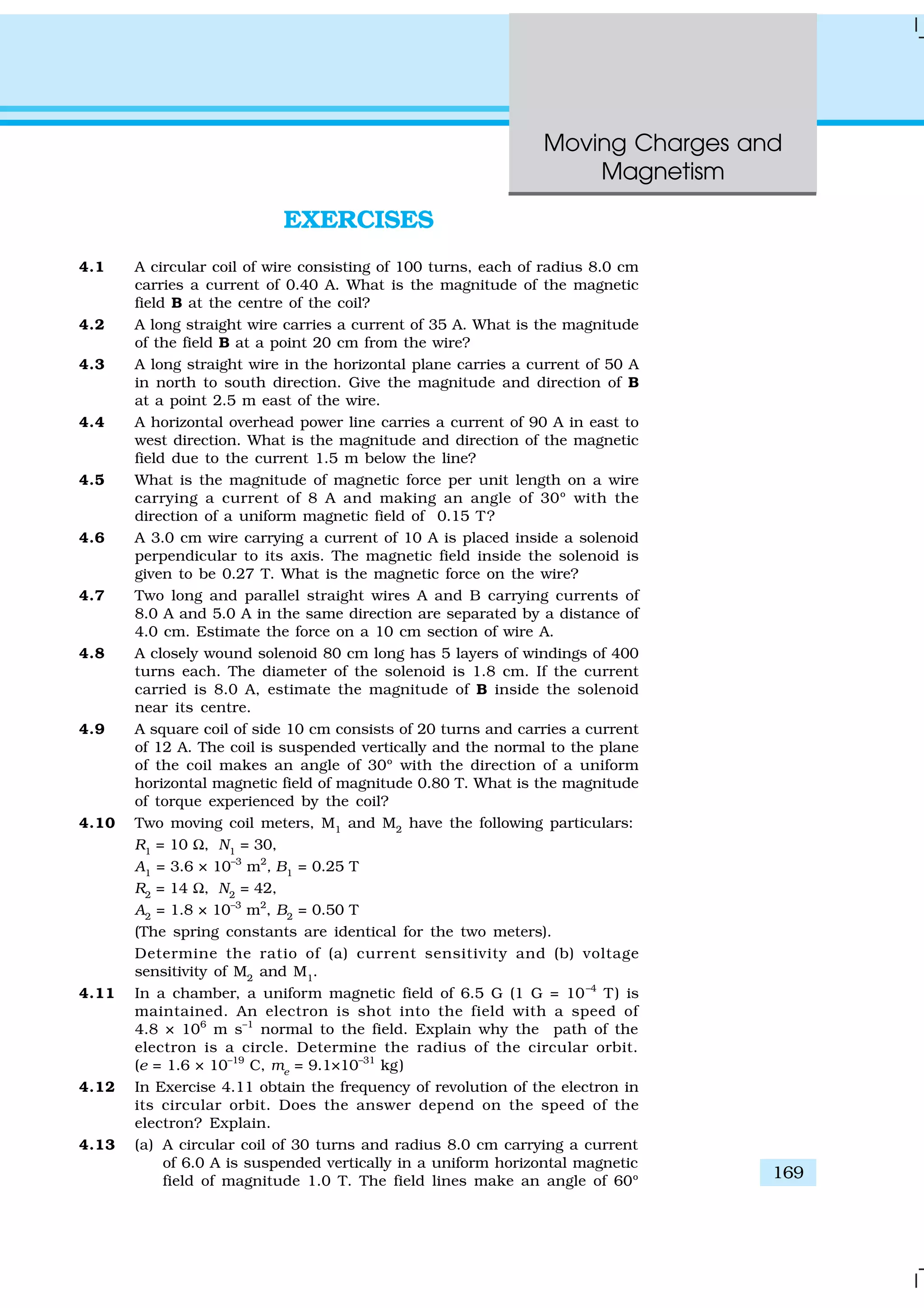
174. Physics
170
with the normal of the coil. Calculate the magnitude of the
counter torque that must be applied to prevent the coil from
turning.
(b) Would your answer change, if the circular coil in (a) were replaced
by a planar coil of some irregular shape that encloses the same
area? (All other particulars are also unaltered.)
ADDITIONAL EXERCISES
4.14 Two concentric circular coils X and Y of radii 16 cm and 10 cm,
respectively, lie in the same vertical plane containing the north to
south direction. Coil X has 20 turns and carries a current of 16 A;
coil Y has 25 turns and carries a current of 18 A. The sense of the
current in X is anticlockwise, and clockwise in Y, for an observer
looking at the coils facing west. Give the magnitude and direction of
the net magnetic field due to the coils at their centre.
4.15 A magnetic field of 100 G (1 G = 10–4
T) is required which is uniform
in a region of linear dimension about 10 cm and area of cross-section
about 10–3
m2
. The maximum current-carrying capacity of a given
coil of wire is 15 A and the number of turns per unit length that can
be wound round a core is at most 1000 turns m–1
. Suggest some
appropriate design particulars of a solenoid for the required purpose.
Assume the core is not ferromagnetic.
4.16 For a circular coil of radius R and N turns carrying current I, the
magnitude of the magnetic field at a point on its axis at a distance x
from its centre is given by,
( )
2
0
3/22 2
2
IR N
B
x R
µ
=
+
(a) Show that this reduces to the familiar result for field at the
centre of the coil.
(b) Consider two parallel co-axial circular coils of equal radius R,
and number of turns N, carrying equal currents in the same
direction, and separated by a distance R. Show that the field on
the axis around the mid-point between the coils is uniform over
a distance that is small as compared to R, and is given by,
0
0.72
NI
B
R
µ
= , approximately.
[Such an arrangement to produce a nearly uniform magnetic
field over a small region is known as Helmholtz coils.]
4.17 A toroid has a core (non-ferromagnetic) of inner radius 25 cm and
outer radius 26 cm, around which 3500 turns of a wire are wound.
If the current in the wire is 11 A, what is the magnetic field
(a) outside the toroid, (b) inside the core of the toroid, and (c) in the
empty space surrounded by the toroid.
4.18 Answer the following questions:
(a) A magnetic field that varies in magnitude from point to point
but has a constant direction (east to west) is set up in a chamber.
A charged particle enters the chamber and travels undeflected

175. Moving Charges and
Magnetism
171
along a straight path with constant speed. What can you say
about the initial velocity of the particle?
(b) A charged particle enters an environment of a strong and
non-uniform magnetic field varying from point to point both in
magnitude and direction, and comes out of it following a
complicated trajectory. Would its final speed equal the initial
speed if it suffered no collisions with the environment?
(c) An electron travelling west to east enters a chamber having a
uniform electrostatic field in north to south direction. Specify
the direction in which a uniform magnetic field should be set
up to prevent the electron from deflecting from its straight line
path.
4.19 An electron emitted by a heated cathode and accelerated through a
potential difference of 2.0 kV, enters a region with uniform magnetic
field of 0.15 T. Determine the trajectory of the electron if the field
(a) is transverse to its initial velocity, (b) makes an angle of 30º with
the initial velocity.
4.20 A magnetic field set up using Helmholtz coils (described in Exercise
4.16) is uniform in a small region and has a magnitude of 0.75 T. In
the same region, a uniform electrostatic field is maintained in a
direction normal to the common axis of the coils. A narrow beam of
(single species) charged particles all accelerated through 15 kV
enters this region in a direction perpendicular to both the axis of
the coils and the electrostatic field. If the beam remains undeflected
when the electrostatic field is 9.0 × 10–5
V m–1
, make a simple guess
as to what the beam contains. Why is the answer not unique?
4.21 A straight horizontal conducting rod of length 0.45 m and mass
60 g is suspended by two vertical wires at its ends. A current of 5.0 A
is set up in the rod through the wires.
(a) What magnetic field should be set up normal to the conductor
in order that the tension in the wires is zero?
(b) What will be the total tension in the wires if the direction of
current is reversed keeping the magnetic field same as before?
(Ignore the mass of the wires.) g = 9.8 m s–2
.
4.22 The wires which connect the battery of an automobile to its starting
motor carry a current of 300 A (for a short time). What is the force
per unit length between the wires if they are 70 cm long and 1.5 cm
apart? Is the force attractive or repulsive?
4.23 A uniform magnetic field of 1.5 T exists in a cylindrical region of
radius10.0 cm, its direction parallel to the axis along east to west. A
wire carrying current of 7.0 A in the north to south direction passes
through this region. What is the magnitude and direction of the
force on the wire if,
(a) the wire intersects the axis,
(b) the wire is turned from N-S to northeast-northwest direction,
(c) the wire in the N-S direction is lowered from the axis by a distance
of 6.0 cm?
4.24 A uniform magnetic field of 3000 G is established along the positive
z-direction. A rectangular loop of sides 10 cm and 5 cm carries a
current of 12 A. What is the torque on the loop in the different cases
shown in Fig. 4.28? What is the force on each case? Which case
corresponds to stable equilibrium?

176. Physics
172
FIGURE 4.28
4.25 A circular coil of 20 turns and radius 10 cm is placed in a uniform
magnetic field of 0.10 T normal to the plane of the coil. If the current
in the coil is 5.0 A, what is the
(a) total torque on the coil,
(b) total force on the coil,
(c) average force on each electron in the coil due to the magnetic
field?
(The coil is made of copper wire of cross-sectional area 10–5
m2
, and
the free electron density in copper is given to be about
1029
m–3
.)
4.26 A solenoid 60 cm long and of radius 4.0 cm has 3 layers of windings
of 300 turns each. A 2.0 cm long wire of mass 2.5 g lies inside the
solenoid (near its centre) normal to its axis; both the wire and the
axis of the solenoid are in the horizontal plane. The wire is connected
through two leads parallel to the axis of the solenoid to an external
battery which supplies a current of 6.0 A in the wire. What value of
current (with appropriate sense of circulation) in the windings of
the solenoid can support the weight of the wire? g = 9.8 m s–2
.
4.27 A galvanometer coil has a resistance of 12 Ω and the metre shows
full scale deflection for a current of 3 mA. How will you convert the
metre into a voltmeter of range 0 to 18 V?
4.28 A galvanometer coil has a resistance of 15 Ω and the metre shows
full scale deflection for a current of 4 mA. How will you convert the
metre into an ammeter of range 0 to 6 A?

177. 5.1 INTRODUCTION
Magnetic phenomena are universal in nature. Vast, distant galaxies, the
tiny invisible atoms, men and beasts all are permeated through and
through with a host of magnetic fields from a variety of sources. The earth’s
magnetism predates human evolution. The word magnet is derived from
the name of an island in Greece called magnesia where magnetic ore
deposits were found, as early as 600 BC. Shepherds on this island
complained that their wooden shoes (which had nails) at times stayed
struck to the ground. Their iron-tipped rods were similarly affected. This
attractive property of magnets made it difficult for them to move around.
The directional property of magnets was also known since ancient
times. A thin long piece of a magnet, when suspended freely, pointed in
the north-south direction. A similar effect was observed when it was placed
on a piece of cork which was then allowed to float in still water. The name
lodestone (or loadstone) given to a naturally occurring ore of iron-
magnetite means leading stone. The technological exploitation of this
property is generally credited to the Chinese. Chinese texts dating 400
BC mention the use of magnetic needles for navigation on ships. Caravans
crossing the Gobi desert also employed magnetic needles.
A Chinese legend narrates the tale of the victory of the emperor Huang-ti
about four thousand years ago, which he owed to his craftsmen (whom
Chapter Five
MAGNETISM AND
MATTER

178. Physics
174
nowadays you would call engineers). These ‘engineers’
built a chariot on which they placed a magnetic figure
with arms outstretched. Figure 5.1 is an artist’s
description of this chariot. The figure swiveled around
so that the finger of the statuette on it always pointed
south. With this chariot, Huang-ti’s troops were able
to attack the enemy from the rear in thick fog, and to
defeat them.
In the previous chapter we have learned that moving
charges or electric currents produce magnetic fields.
This discovery, which was made in the early part of the
nineteenth century is credited to Oersted, Ampere, Biot
and Savart, among others.
In the present chapter, we take a look at magnetism
as a subject in its own right.
Some of the commonly known ideas regarding
magnetism are:
(i) The earth behaves as a magnet with the magnetic
field pointing approximately from the geographic
south to the north.
(ii) When a bar magnet is freely suspended, it points in the north-south
direction. The tip which points to the geographic north is called the
north pole and the tip which points to the geographic south is called
the south pole of the magnet.
(iii) There is a repulsive force when north poles ( or south poles ) of two
magnets are brought close together. Conversely, there is an attractive
force between the north pole of one magnet and the south pole of
the other.
(iv) We cannot isolate the north, or south pole of a magnet. If a bar magnet
is broken into two halves, we get two similar bar magnets with
somewhat weaker properties. Unlike electric charges, isolated magnetic
north and south poles known as magnetic monopoles do not exist.
(v) It is possible to make magnets out of iron and its alloys.
We begin with a description of a bar magnet and its behaviour in an
external magnetic field. We describe Gauss’s law of magnetism. We then
follow it up with an account of the earth’s magnetic field. We next describe
how materials can be classified on the basis of their magnetic properties.
We describe para-, dia-, and ferromagnetism. We conclude with a section
on electromagnets and permanent magnets.
5.2 THE BAR MAGNET
One of the earliest childhood memories of the famous physicist Albert
Einstein was that of a magnet gifted to him by a relative. Einstein was
fascinated, and played endlessly with it. He wondered how the magnet
could affect objects such as nails or pins placed away from it and not in
any way connected to it by a spring or string.
FIGURE 5.1 The arm of the statuette
mounted on the chariot always points
south. This is an artist’s sketch of one
of the earliest known compasses,
thousands of years old.

179. Magnetism and
Matter
175
We begin our study by examining iron filings sprinkled on a sheet of
glass placed over a short bar magnet. The arrangement of iron filings is
shown in Fig. 5.2.
The pattern of iron filings suggests that the magnet has two poles
similar to the positive and negative charge of an electric dipole. As
mentioned in the introductory section, one pole is designated the North
pole and the other, the South pole. When suspended freely, these poles
point approximately towards the geographic north and south poles,
respectively. A similar pattern of iron filings is observed around a current
carrying solenoid.
5.2.1 The magnetic field lines
The pattern of iron filings permits us to plot the magnetic field lines*. This is
shown both for the bar-magnet and the current-carrying solenoid in
Fig. 5.3. For comparison refer to the Chapter 1, Figure 1.17(d). Electric field
lines of an electric dipole are also displayed in Fig. 5.3(c). The magnetic field
lines are a visual and intuitive realisation of the magnetic field. Their
properties are:
(i) The magnetic field lines of a magnet (or a solenoid) form continuous
closed loops. This is unlike the electric dipole where these field lines
begin from a positive charge and end on the negative charge or escape
to infinity.
(ii) The tangent to the field line at a given point represents the direction of
the net magnetic field B at that point.
FIGURE 5.2 The
arrangement of iron
filings surrounding a
bar magnet. The
pattern mimics
magnetic field lines.
The pattern suggests
that the bar magnet
is a magnetic dipole.
* In some textbooks the magnetic field lines are called magnetic lines of force.
This nomenclature is avoided since it can be confusing. Unlike electrostatics
the field lines in magnetism do not indicate the direction of the force on a
(moving) charge.
FIGURE 5.3 The field lines of (a) a bar magnet, (b) a current-carrying finite solenoid and
(c) electric dipole. At large distances, the field lines are very similar. The curves
labelled i and ii are closed Gaussian surfaces.

180. Physics
176
(iii) The larger the number of field lines crossing per unit area, the stronger
is the magnitude of the magnetic field B. In Fig. 5.3(a), B is larger
around region ii than in region i .
(iv) The magnetic field lines do not intersect, for if they did, the direction
of the magnetic field would not be unique at the point of intersection.
One can plot the magnetic field lines in a variety of ways. One way is
to place a small magnetic compass needle at various positions and note
its orientation. This gives us an idea of the magnetic field direction at
various points in space.
5.2.2 Bar magnet as an equivalent solenoid
In the previous chapter, we have explained how a current loop acts as a
magnetic dipole (Section 4.10). We mentioned Ampere’s hypothesis that
all magnetic phenomena can be explained in terms of circulating currents.
Recall that the magnetic dipole moment m
associated with a current loop was defined
to be m = NIA where N is the number of
turns in the loop, I the current and A the
area vector (Eq. 4.30).
The resemblance of magnetic field lines
for a bar magnet and a solenoid suggest that
a bar magnet may be thought of as a large
number of circulating currents in analogy
with a solenoid. Cutting a bar magnet in half
is like cutting a solenoid. We get two smaller
solenoids with weaker magnetic properties.
The field lines remain continuous, emerging
from one face of the solenoid and entering
into the other face. One can test this analogy
by moving a small compass needle in the
neighbourhood of a bar magnet and a
current-carrying finite solenoid and noting
that the deflections of the needle are similar
in both cases.
To make this analogy more firm we
calculate the axial field of a finite solenoid
depicted in Fig. 5.4 (a). We shall demonstrate
that at large distances this axial field
resembles that of a bar magnet.
Let the solenoid of Fig. 5.4(a) consists of
n turns per unit length. Let its length be 2l
and radius a. We can evaluate the axial field
at a point P, at a distance r from the centre O
of the solenoid. To do this, consider a circular element of thickness dx of
the solenoid at a distance x from its centre. It consists of n d x turns. Let
I be the current in the solenoid. In Section 4.6 of the previous chapter we
have calculated the magnetic field on the axis of a circular current loop.
From Eq. (4.13), the magnitude of the field at point P due to the circular
element is
FIGURE 5.4 (a) Calculation of the axial field of a
finite solenoid in order to demonstrate its similarity
to that of a bar magnet. (b) A magnetic needle
in a uniform magnetic field B. The
arrangement may be used to
determine either B or the magnetic
moment m of the needle.

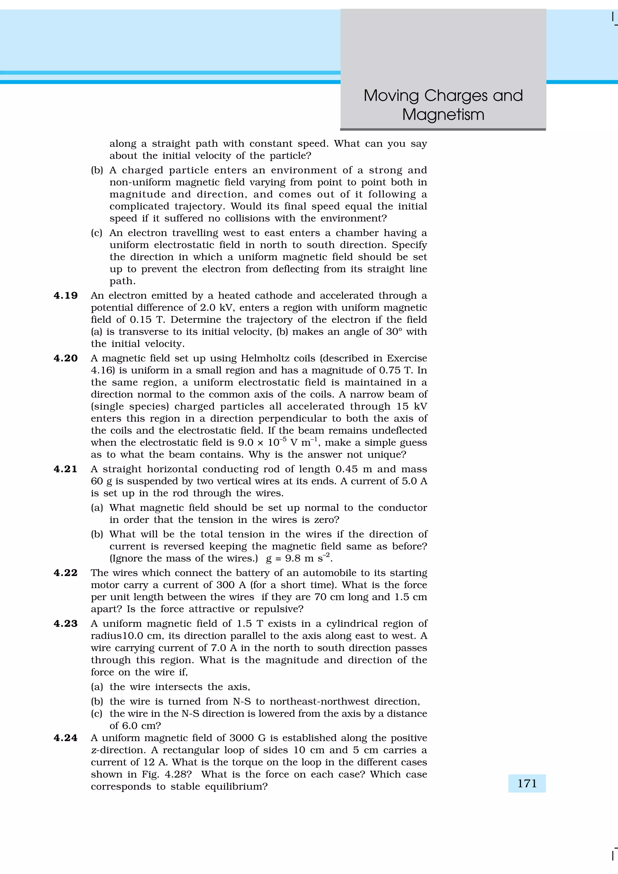
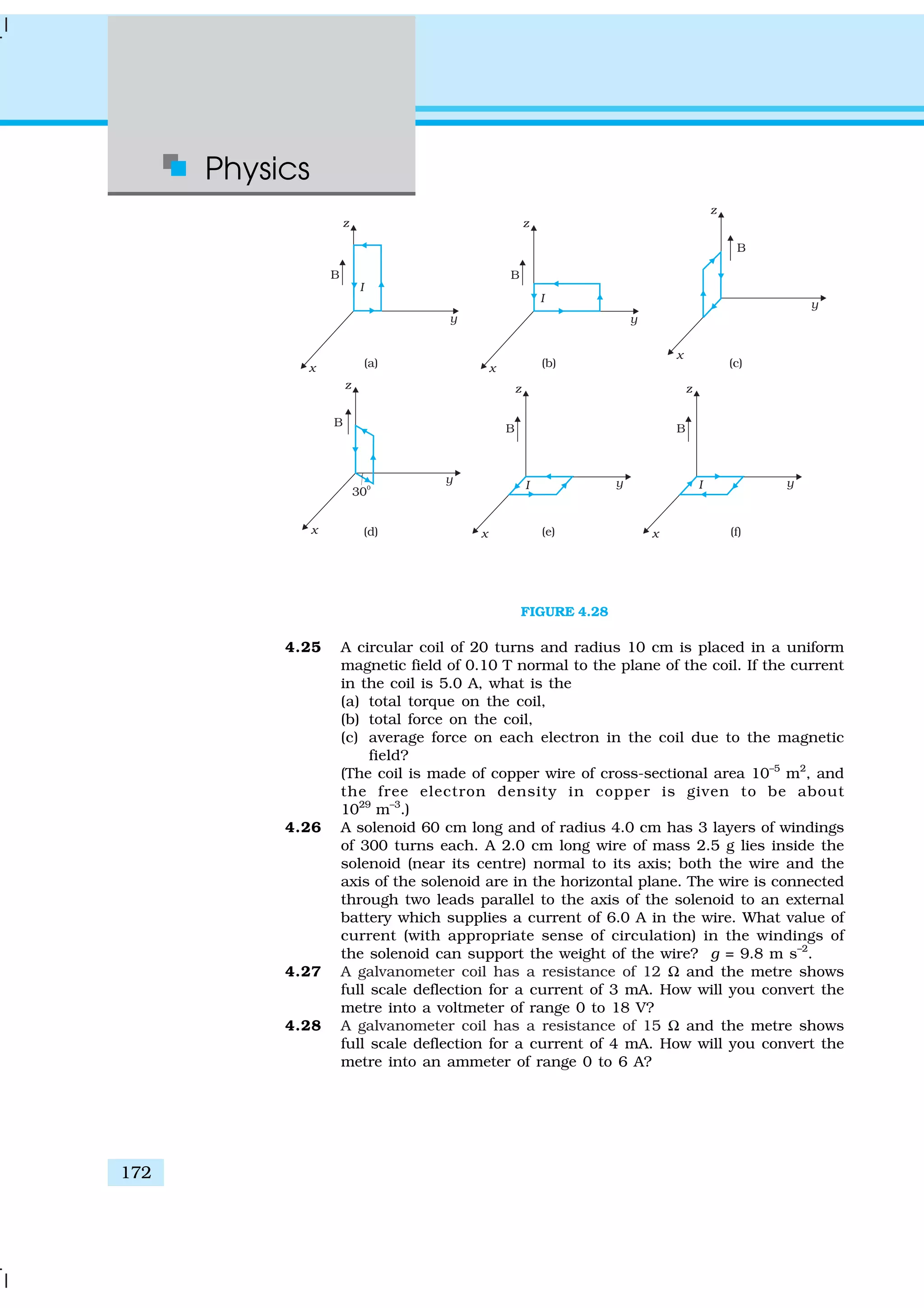
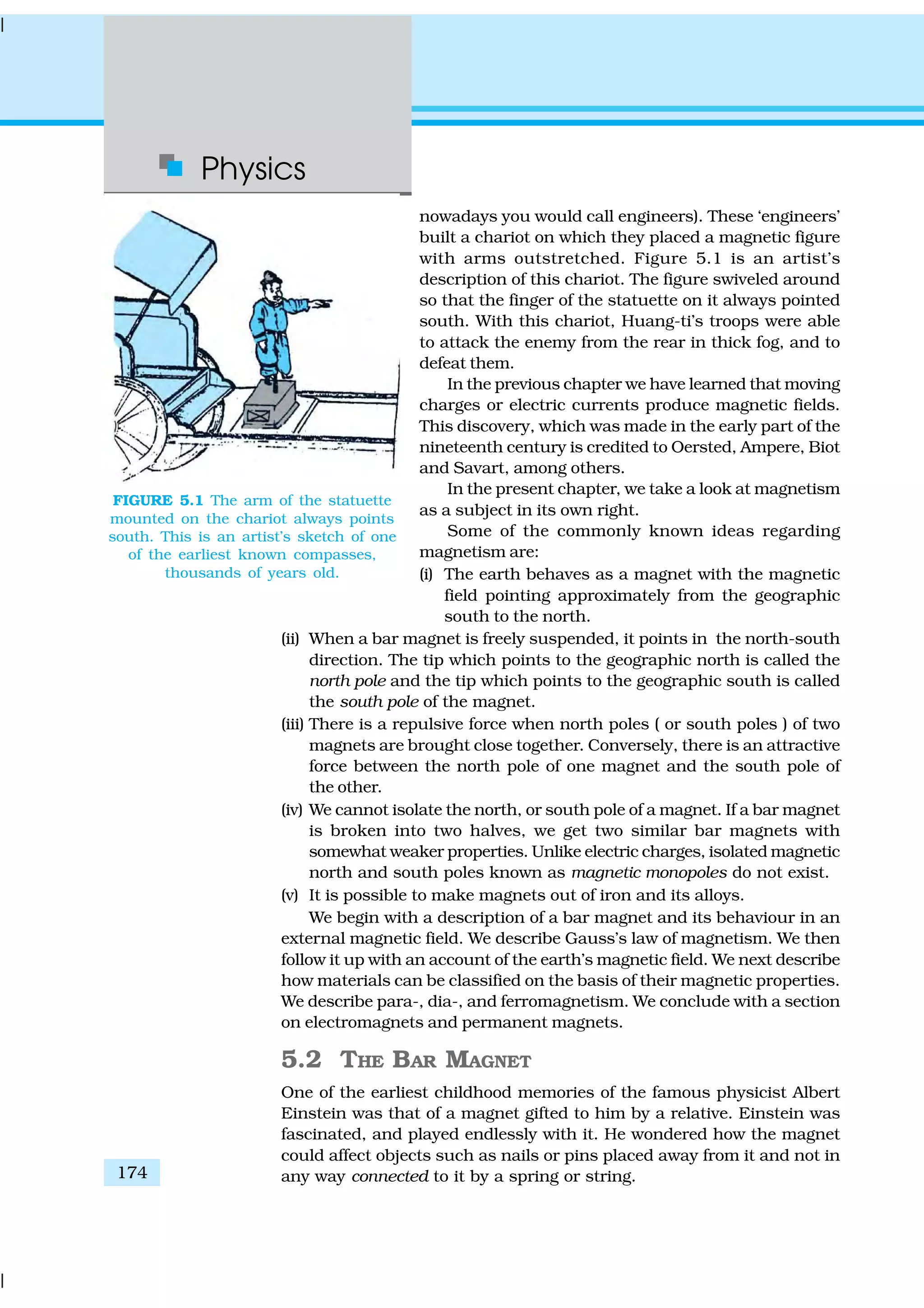
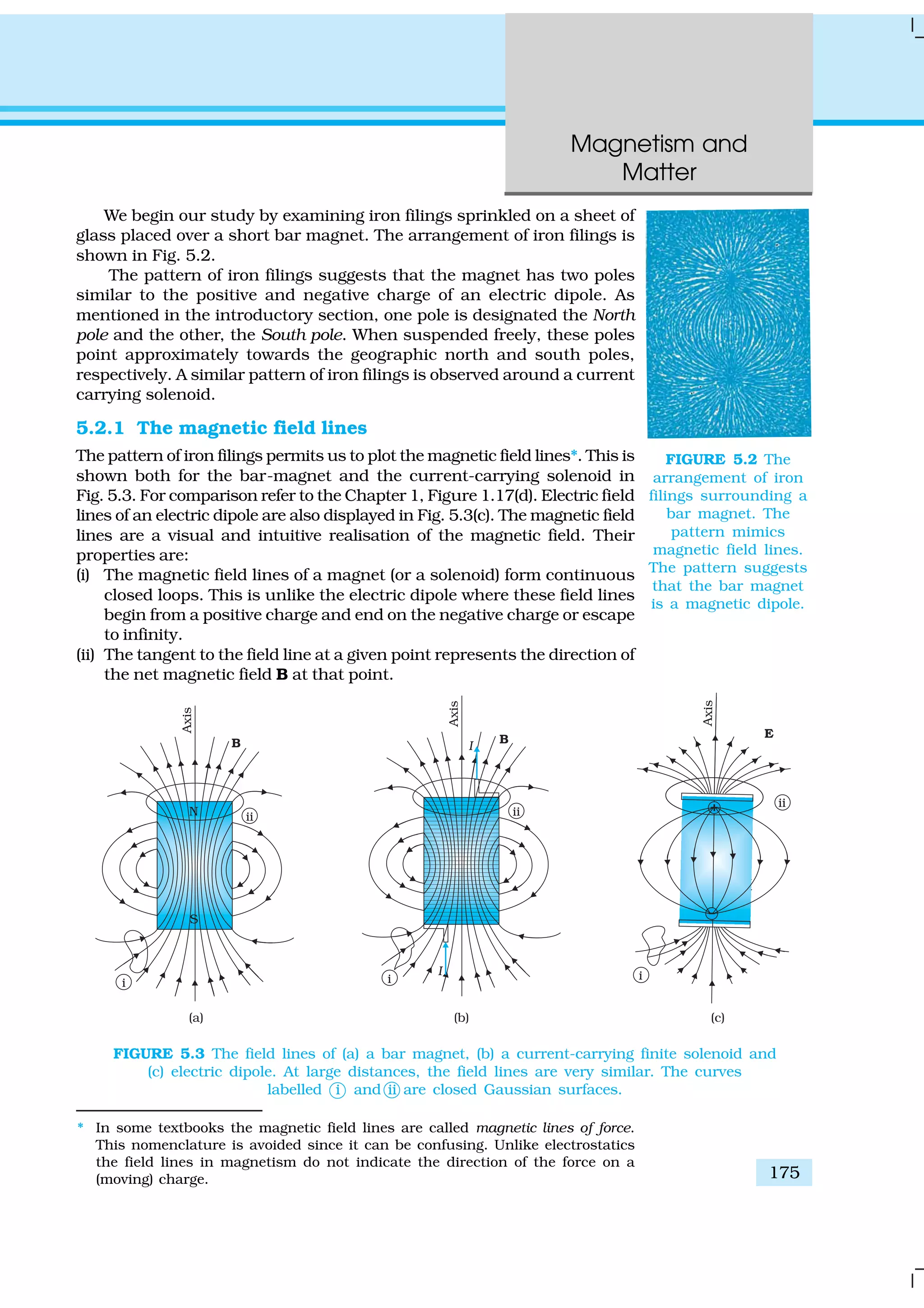
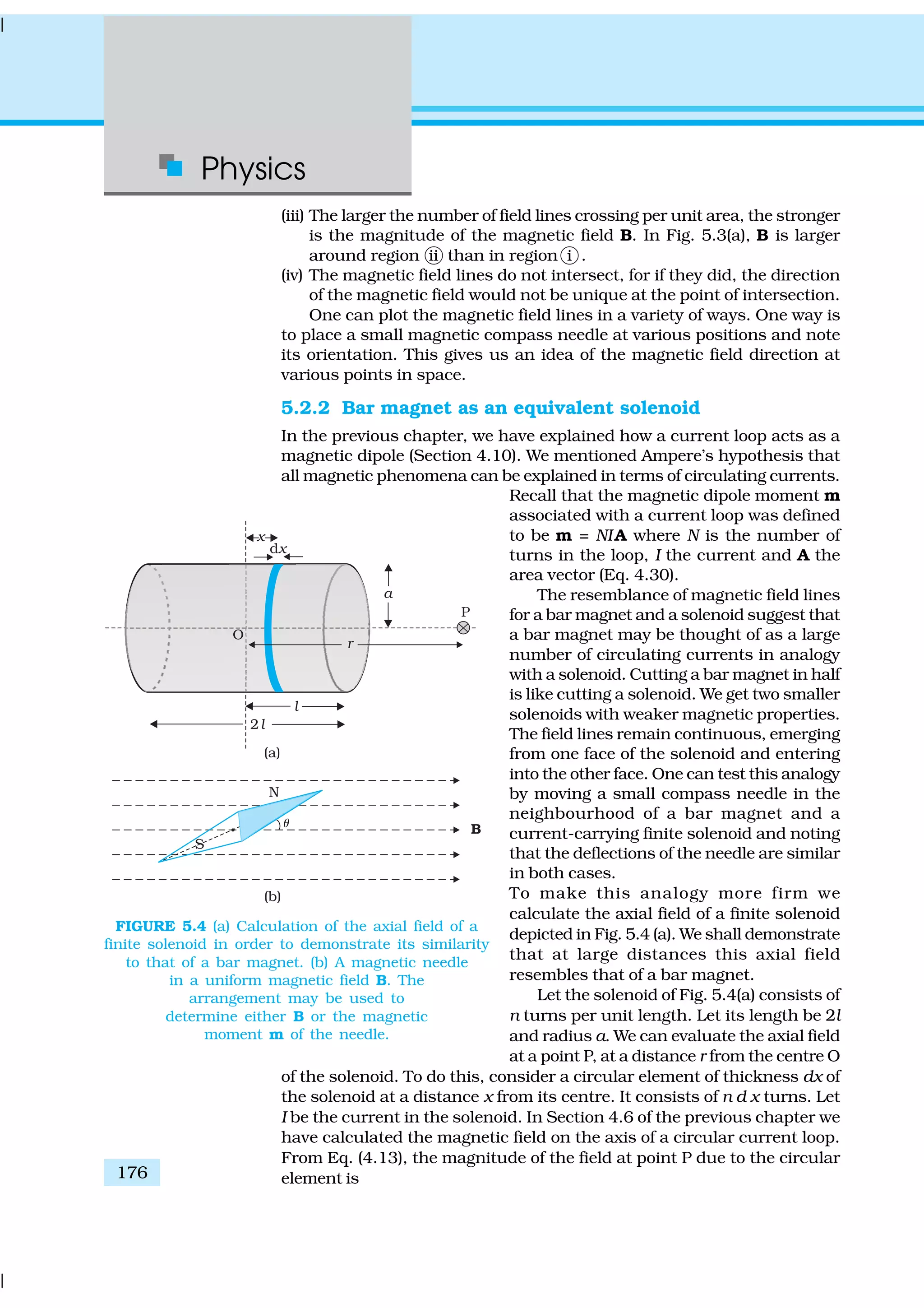
181. Magnetism and
Matter
177
2
0
3
2 2 2
2[( ) ]
n dx I a
dB
r x a
µ
=
− +
The magnitude of the total field is obtained by summing over all the
elements — in other words by integrating from x = – l to x = + l. Thus,
2
0
2
nIa
B
µ
= 2 2 3/2
[( ) ]
l
l
dx
r x a− − +∫
This integration can be done by trigonometric substitutions. This
exercise, however, is not necessary for our purpose. Note that the range
of x is from – l to + l. Consider the far axial field of the solenoid, i.e.,
r >> a and r >> l. Then the denominator is approximated by
3
2 2 32
[( ) ]r x a r− + ≈
and
2
0
3
2
l
l
n I a
B dx
r
µ
−
= ∫
=
2
0
3
2
2
n I l a
r
µ
(5.1)
Note that the magnitude of the magnetic moment of the solenoid is,
m = n (2l) I (πa2
) — (total number of turns × current × cross-sectional
area). Thus,
0
3
2
4
m
B
r
µ
π
= (5.2)
This is also the far axial magnetic field of a bar magnet which one may
obtain experimentally. Thus, a bar magnet and a solenoid produce similar
magnetic fields. The magnetic moment of a bar magnet is thus equal to
the magnetic moment of an equivalent solenoid that produces the same
magnetic field.
Some textbooks assign a magnetic charge (also called pole strength)
+qm
to the north pole and –qm
to the south pole of a bar magnet of length
2l, and magnetic moment qm
(2l). The field strength due to qm
at a distance
r from it is given by µ0qm/4πr2
. The magnetic field due to the bar magnet
is then obtained, both for the axial and the equatorial case, in a manner
analogous to that of an electric dipole (Chapter 1). The method is simple
and appealing. However, magnetic monopoles do not exist, and we have
avoided this approach for that reason.
5.2.3 The dipole in a uniform magnetic field
The pattern of iron filings, i.e., the magnetic field lines gives us an
approximate idea of the magnetic field B. We may at times be required to
determine the magnitude of B accurately. This is done by placing a small
compass needle of known magnetic moment m and moment of inertia 1
and allowing it to oscillate in the magnetic field. This arrangement is shown
in Fig. 5.4(b).
The torque on the needle is [see Eq. (4.29)],
τ = m × B (5.3)

182. Physics
178
EXAMPLE5.1
In magnitude τ = mB sinθ
Here ττ is restoring torque and θ is the angle between m and B.
Therefore, in equilibrium
2
2
sin
d
mB
dt
θ
θ= −1
Negative sign with mB sinθ implies that restoring torque is in opposition
to deflecting torque. For small values of θ in radians, we approximate
sin θ ≈ θ and get
2
2
–
d
mB
dt
θ
θ≈1
or,
2
2
d mB
dt
θ
θ= −
1
This represents a simple harmonic motion. The square of the angular
frequency is ω2
= mB/1 and the time period is,
2T
mB
π=
1
(5.4)
or
4 2
2
B
m T
π
=
1
(5.5)
An expression for magnetic potential energy can also be obtained on
lines similar to electrostatic potential energy.
The magnetic potential energy Um
is given by
( )mU dτ θ θ= ∫
sinmB θ= ∫ cosmB θ= −
= −m Bg (5.6)
We have emphasised in Chapter 2 that the zero of potential energy
can be fixed at one’s convenience. Taking the constant of integration to be
zero means fixing the zero of potential energy at θ = 90º, i.e., when the
needle is perpendicular to the field. Equation (5.6) shows that potential
energy is minimum (= –mB) at θ = 0º (most stable position) and maximum
(= +mB) at θ = 180º (most unstable position).
Example 5.1 In Fig. 5.4(b), the magnetic needle has magnetic moment
6.7 × 10–2
Am2
and moment of inertia 1 = 7.5 × 10–6
kg m2
. It performs
10 complete oscillations in 6.70 s. What is the magnitude of the
magnetic field?
Solution The time period of oscillation is,
6.70
0.67
10
T s= =
From Eq. (5.5)
2
2
4
B
mT
π
=
1
=
2 6
–2 2
4 (3.14) 7.5 10
6.7 10 (0.67)
−
× × ×
× ×
= 0.01 T

183. Magnetism and
Matter
179
EXAMPLE5.2
Example 5.2 A short bar magnet placed with its axis at 30º with an
external field of 800 G experiences a torque of 0.016 Nm. (a) What is
the magnetic moment of the magnet? (b) What is the work done in
moving it from its most stable to most unstable position? (c) The bar
magnet is replaced by a solenoid of cross-sectional area 2 × 10–4
m2
and 1000 turns, but of the same magnetic moment. Determine the
current flowing through the solenoid.
Solution
(a) From Eq. (5.3), τ = m B sin θ, θ = 30º, hence sinθ =1/2.
Thus, 0.016 = m × (800 × 10–4
T) × (1/2)
m = 160 × 2/800 = 0.40 A m2
(b) From Eq. (5.6), the most stable position is θ = 0º and the most
unstable position is θ = 180º. Work done is given by
( 180 ) ( 0 )m mW U Uθ θ= = ° − = °
= 2 m B = 2 × 0.40 × 800 × 10–4
= 0.064 J
(c) From Eq. (4.30), ms
= NIA. From part (a), ms
= 0.40 A m2
0.40 = 1000 × I × 2 × 10–4
I = 0.40 × 104
/(1000 × 2) = 2A
Example 5.3
(a) What happens if a bar magnet is cut into two pieces: (i) transverse
to its length, (ii) along its length?
(b) A magnetised needle in a uniform magnetic field experiences a
torque but no net force. An iron nail near a bar magnet, however,
experiences a force of attraction in addition to a torque. Why?
(c) Must every magnetic configuration have a north pole and a south
pole? What about the field due to a toroid?
(d) Two identical looking iron bars A and B are given, one of which is
definitely known to be magnetised. (We do not know which one.)
How would one ascertain whether or not both are magnetised? If
only one is magnetised, how does one ascertain which one? [Use
nothing else but the bars A and B.]
Solution
(a) In either case, one gets two magnets, each with a north and south
pole.
(b) No force if the field is uniform. The iron nail experiences a non-
uniform field due to the bar magnet. There is induced magnetic
moment in the nail, therefore, it experiences both force and torque.
The net force is attractive because the induced south pole (say) in
the nail is closer to the north pole of magnet than induced north
pole.
(c) Not necessarily. True only if the source of the field has a net non-
zero magnetic moment. This is not so for a toroid or even for a
straight infinite conductor.
(d) Try to bring different ends of the bars closer. A repulsive force in
some situation establishes that both are magnetised. If it is always
attractive, then one of them is not magnetised. In a bar magnet
the intensity of the magnetic field is the strongest at the two ends
(poles) and weakest at the central region. This fact may be used to
determine whether A or B is the magnet. In this case, to see which
EXAMPLE5.3

184. Physics
180
EXAMPLE5.4EXAMPLE5.3
one of the two bars is a magnet, pick up one, (say, A) and lower one of
its ends; first on one of the ends of the other (say, B), and then on the
middle of B. If you notice that in the middle of B, A experiences no
force, then B is magnetised. If you do not notice any change from the
end to the middle of B, then A is magnetised.
5.2.4 The electrostatic analog
Comparison of Eqs. (5.2), (5.3) and (5.6) with the corresponding equations
for electric dipole (Chapter 1), suggests that magnetic field at large
distances due to a bar magnet of magnetic moment m can be obtained
from the equation for electric field due to an electric dipole of dipole moment
p, by making the following replacements:
→E B , →p m ,
0
0
1
4 4
µ
ε
→
π π
In particular, we can write down the equatorial field (BE) of a bar magnet
at a distance r, for r >> l, where l is the size of the magnet:
0
3
4
E
r
µ
= −
π
m
B (5.7)
Likewise, the axial field (BA) of a bar magnet for r >> l is:
0
3
2
4
A
r
µ
=
π
m
B (5.8)
Equation (5.8) is just Eq. (5.2) in the vector form. Table 5.1 summarises
the analogy between electric and magnetic dipoles.
Electrostatics Magnetism
1/ε0
µ0
Dipole moment p m
Equatorial Field for a short dipole –p/4πε0
r3
– µ0
m / 4π r3
Axial Field for a short dipole 2p/4πε0
r3
µ0
2m / 4π r3
External Field: torque p × E m × B
External Field: Energy –p.E –m.B
TABLE 5.1 THE DIPOLE ANALOGY
Example 5.4 What is the magnitude of the equatorial and axial fields
due to a bar magnet of length 5.0 cm at a distance of 50 cm from its
mid-point? The magnetic moment of the bar magnet is 0.40 A m2
, the
same as in Example 5.2.
Solution From Eq. (5.7)
0
3
4
E
m
B
r
µ
=
π ( )
7 7
3
10 0.4 10 0.4
0.1250.5
− −
× ×
= = 7
3.2 10 T−
= ×
From Eq. (5.8),
0
3
2
4
A
m
B
r
µ
=
π
7
6.4 10 T−
= ×

185. Magnetism and
Matter
181
EXAMPLE5.5
Example 5.5 Figure 5.5 shows a small magnetised needle P placed at
a point O. The arrow shows the direction of its magnetic moment. The
other arrows show different positions (and orientations of the magnetic
moment) of another identical magnetised needle Q.
(a) In which configuration the system is not in equilibrium?
(b) In which configuration is the system in (i) stable, and (ii) unstable
equilibrium?
(c) Which configuration corresponds to the lowest potential energy
among all the configurations shown?
FIGURE 5.5
Solution
Potential energy of the configuration arises due to the potential energy of
one dipole (say, Q) in the magnetic field due to other (P). Use the result
that the field due to P is given by the expression [Eqs. (5.7) and (5.8)]:
0 P
P 3
4 r
µ
π
= −
m
B (on the normal bisector)
0 P
P 3
2
4 r
µ
π
=
m
B (on the axis)
where mP
is the magnetic moment of the dipole P.
Equilibrium is stable when mQ
is parallel to BP
, and unstable when it
is anti-parallel to BP
.
For instance for the configuration Q3
for which Q is along the
perpendicular bisector of the dipole P, the magnetic moment of Q is
parallel to the magnetic field at the position 3. Hence Q3
is stable.
Thus,
(a) PQ1
and PQ2
(b) (i) PQ3
, PQ6
(stable); (ii) PQ5
, PQ4
(unstable)
(c) PQ6
5.3 MAGNETISM AND GAUSS’S LAW
In Chapter 1, we studied Gauss’s law for electrostatics. In Fig 5.3(c), we
see that for a closed surface represented by i , the number of lines leaving
the surface is equal to the number of lines entering it. This is consistent
with the fact that no net charge is enclosed by the surface. However, in
the same figure, for the closed surface ii, thereis a net outward flux, since
it does include a net (positive) charge.

186. Physics
182
EXAMPLE5.6
The situation is radically different for magnetic fields
which are continuous and form closed loops. Examine the
Gaussian surfaces represented by i or ii in Fig 5.3(a) or
Fig. 5.3(b). Both cases visually demonstrate that the
number of magnetic field lines leaving the surface is
balanced by the number of lines entering it. The net
magnetic flux is zero for both the surfaces. This is true
for any closed surface.
FIGURE 5.6
Consider a small vector area element ∆S of a closed
surface S as in Fig. 5.6. The magnetic flux through ÄS is
defined as ∆φB
= B.∆S, where B is the field at ∆S. We divide
S into many small area elements and calculate the
individual flux through each. Then, the net flux φB
is,
' ' ' '
0B B
all all
φ φ= ∆ = ∆ =∑ ∑B Sg (5.9)
where ‘all’ stands for ‘all area elements ∆S′. Compare this
with the Gauss’s law of electrostatics. The flux through a closed surface
in that case is given by
0
q
∆ =
ε
∑E Sg
where q is the electric charge enclosed by the surface.
The difference between the Gauss’s law of magnetism and that for
electrostatics is a reflection of the fact that isolated magnetic poles (also
called monopoles) are not known to exist. There are no sources or sinks
of B; the simplest magnetic element is a dipole or a current loop. All
magnetic phenomena can be explained in terms of an arrangement of
dipoles and/or current loops.
Thus, Gauss’s law for magnetism is:
The net magnetic flux through any closed surface is zero.
Example 5.6 Many of the diagrams given in Fig. 5.7 show magnetic
field lines (thick lines in the figure) wrongly. Point out what is wrong
with them. Some of them may describe electrostatic field lines correctly.
Point out which ones.
KARLFRIEDRICHGAUSS(1777–1855)
Karl Friedrich Gauss
(1777 – 1855) He was a
child prodigy and was gifted
in mathematics, physics,
engineering, astronomy
and even land surveying.
The properties of numbers
fascinated him, and in his
work he anticipated major
mathematical development
of later times. Along with
Wilhelm Welser, he built the
first electric telegraph in
1833. His mathematical
theory of curved surface
laid the foundation for the
later work of Riemann.

187. Magnetism and
Matter
183
EXAMPLE5.6
FIGURE 5.7
Solution
(a) Wrong. Magnetic field lines can never emanate from a point, as
shown in figure. Over any closed surface, the net flux of B must
always be zero, i.e., pictorially as many field lines should seem to
enter the surface as the number of lines leaving it. The field lines
shown, in fact, represent electric field of a long positively charged
wire. The correct magnetic field lines are circling the straight
conductor, as described in Chapter 4.

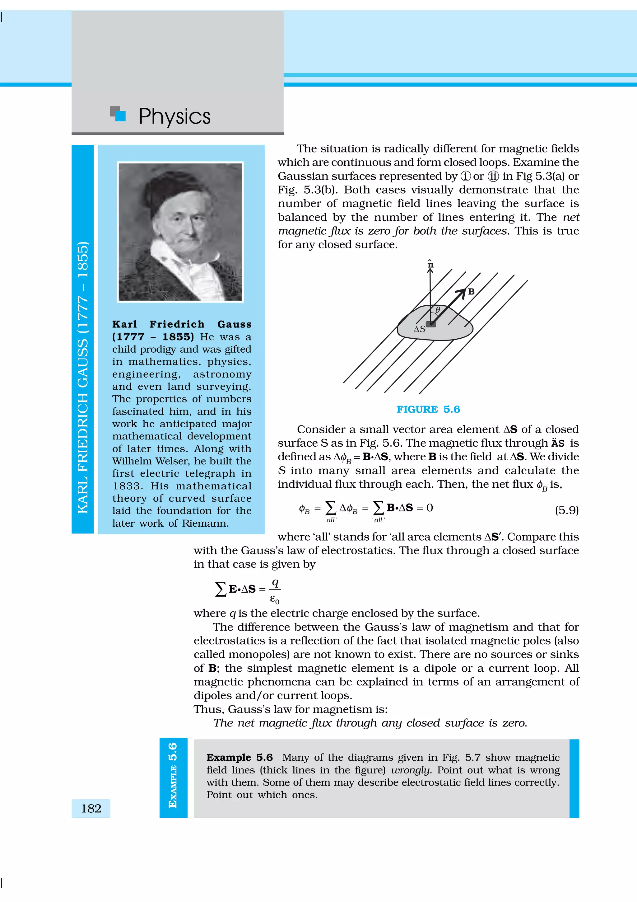
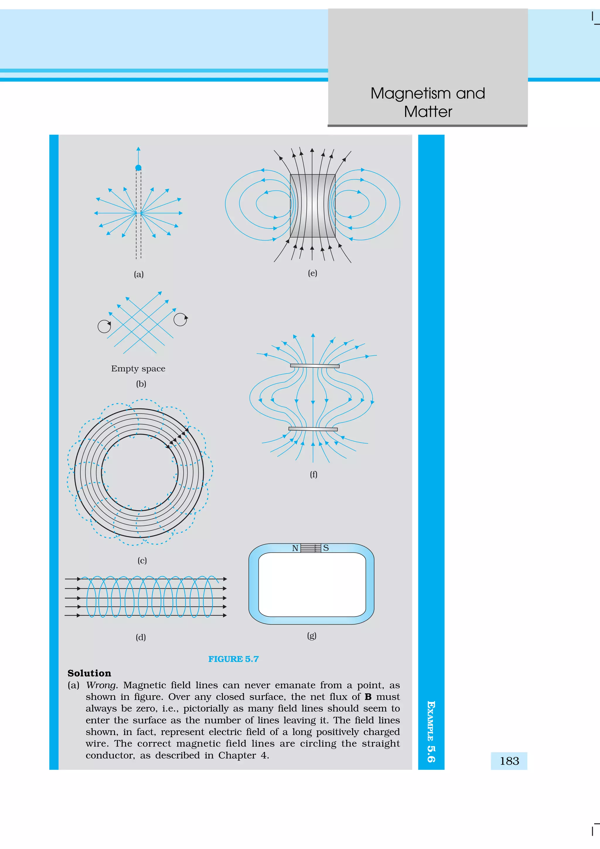
188. Physics
184
EXAMPLE5.7EXAMPLE5.6
(b) Wrong. Magnetic field lines (like electric field lines) can never cross
each other, because otherwise the direction of field at the point of
intersection is ambiguous. There is further error in the figure.
Magnetostatic field lines can never form closed loops around empty
space. A closed loop of static magnetic field line must enclose a
region across which a current is passing. By contrast, electrostatic
field lines can never form closed loops, neither in empty space,
nor when the loop encloses charges.
(c) Right. Magnetic lines are completely confined within a toroid.
Nothing wrong here in field lines forming closed loops, since each
loop encloses a region across which a current passes. Note, for
clarity of figure, only a few field lines within the toroid have been
shown. Actually, the entire region enclosed by the windings
contains magnetic field.
(d) Wrong. Field lines due to a solenoid at its ends and outside cannot
be so completely straight and confined; such a thing violates
Ampere’s law. The lines should curve out at both ends, and meet
eventually to form closed loops.
(e) Right. These are field lines outside and inside a bar magnet. Note
carefully the direction of field lines inside. Not all field lines emanate
out of a north pole (or converge into a south pole). Around both
the N-pole, and the S-pole, the net flux of the field is zero.
(f ) Wrong. These field lines cannot possibly represent a magnetic field.
Look at the upper region. All the field lines seem to emanate out of
the shaded plate. The net flux through a surface surrounding the
shaded plate is not zero. This is impossible for a magnetic field.
The given field lines, in fact, show the electrostatic field lines
around a positively charged upper plate and a negatively charged
lower plate. The difference between Fig. [5.7(e) and (f)] should be
carefully grasped.
(g) Wrong. Magnetic field lines between two pole pieces cannot be
precisely straight at the ends. Some fringing of lines is inevitable.
Otherwise, Ampere’s law is violated. This is also true for electric
field lines.
Example 5.7
(a) Magnetic field lines show the direction (at every point) along which
a small magnetised needle aligns (at the point). Do the magnetic
field lines also represent the lines of force on a moving charged
particle at every point?
(b) Magnetic field lines can be entirely confined within the core of a
toroid, but not within a straight solenoid. Why?
(c) If magnetic monopoles existed, how would the Gauss’s law of
magnetism be modified?
(d) Does a bar magnet exert a torque on itself due to its own field?
Does one element of a current-carrying wire exert a force on another
element of the same wire?
(e) Magnetic field arises due to charges in motion. Can a system have
magnetic moments even though its net charge is zero?
Solution
(a) No. The magnetic force is always normal to B (remember magnetic
force = qv × B). It is misleading to call magnetic field lines as lines
of force.

189. Magnetism and
Matter
185
EXAMPLE5.7
(b) If field lines were entirely confined between two ends of a straight
solenoid, the flux through the cross-section at each end would be
non-zero. But the flux of field B through any closed surface must
always be zero. For a toroid, this difficulty is absent because it
has no ‘ends’.
(c) Gauss’s law of magnetism states that the flux of B through any
closed surface is always zero 0
S
d =∫ B sgÑ .
If monopoles existed, the right hand side would be equal to the
monopole (magnetic charge) qm
enclosed by S. [Analogous to
Gauss’s law of electrostatics, 0 mS
d qµ=∫ B sg where qm
is the
(monopole) magnetic charge enclosed by S.]
(d) No. There is no force or torque on an element due to the field
produced by that element itself. But there is a force (or torque) on
an element of the same wire. (For the special case of a straight
wire, this force is zero.)
(e) Yes. The average of the charge in the system may be zero. Yet, the
mean of the magnetic moments due to various current loops may
not be zero. We will come across such examples in connection
with paramagnetic material where atoms have net dipole moment
through their net charge is zero.
5.4 THE EARTH’S MAGNETISM
Earlier we have referred to the magnetic field of the earth. The strength of
the earth’s magnetic field varies from place to place on the earth’s surface;
its value being of the order of 10–5
T.
What causes the earth to have a magnetic field is not clear. Originally
the magnetic field was thought of as arising from a giant bar magnet
placed approximately along the axis of rotation of the earth and deep in
the interior. However, this simplistic picture is certainly not correct. The
magnetic field is now thought to arise due to electrical currents produced
by convective motion of metallic fluids (consisting mostly of molten
iron and nickel) in the outer core of the earth. This is known as the
dynamo effect.
The magnetic field lines of the earth resemble that of a (hypothetical)
magnetic dipole located at the centre of the earth. The axis of the dipole
does not coincide with the axis of rotation of the earth but is presently
titled by approximately 11.3º with respect to the later. In this way of looking
at it, the magnetic poles are located where the magnetic field lines due to
the dipole enter or leave the earth. The location of the north magnetic pole
is at a latitude of 79.74º N and a longitude of 71.8º W, a place somewhere
in north Canada. The magnetic south pole is at 79.74º S, 108.22º E in the
Antarctica.
The pole near the geographic north pole of the earth is called the north
magnetic pole. Likewise, the pole near the geographic south pole is called
oneldioGeomagneticfieldfrequentlyaskedquestions
http://www.ngdc.noaa.gov/seg/geomag/

190. Physics
186
EXAMPLE5.8
the south magnetic pole. There is some confusion in the
nomenclature of the poles. If one looks at the magnetic
field lines of the earth (Fig. 5.8), one sees that unlike in the
case of a bar magnet, the field lines go into the earth at the
north magnetic pole (Nm) and come out from the south
magnetic pole (Sm
). The convention arose because the
magnetic north was the direction to which the north
pole of a magnetic needle pointed; the north pole of
a magnet was so named as it was the north seeking
pole. Thus, in reality, the north magnetic pole behaves
like the south pole of a bar magnet inside the earth and
vice versa.
Example 5.8 The earth’s magnetic field at the equator is approximately
0.4 G. Estimate the earth’s dipole moment.
Solution From Eq. (5.7), the equatorial magnetic field is,
0
3
4
E
m
B
r
µ
=
π
We are given that BE
~ 0.4 G = 4 × 10–5
T. For r, we take the radius of
the earth 6.4 × 106
m. Hence,
5 6 3
0
4 10 (6.4 10 )
/4
m
µ
−
× × ×
=
π
=4 × 102
× (6.4 × 106
)3
(µ0
/4π = 10–7
)
= 1.05 × 1023
A m2
This is close to the value 8 × 1022
A m2
quoted in geomagnetic texts.
5.4.1 Magnetic declination and dip
Consider a point on the earth’s surface. At such a point, the direction of
the longitude circle determines the geographic north-south direction, the
line of longitude towards the north pole being the direction of
true north. The vertical plane containing the longitude circle
and the axis of rotation of the earth is called the geographic
meridian. In a similar way, one can define magnetic meridian
of a place as the vertical plane which passes through the
imaginary line joining the magnetic north and the south poles.
This plane would intersect the surface of the earth in a
longitude like circle. A magnetic needle, which is free to swing
horizontally, would then lie in the magnetic meridian and the
north pole of the needle would point towards the magnetic
north pole. Since the line joining the magnetic poles is titled
with respect to the geographic axis of the earth, the magnetic
meridian at a point makes angle with the geographic meridian.
This, then, is the angle between the true geographic north and
the north shown by a compass needle. This angle is called the
magnetic declination or simply declination (Fig. 5.9).
The declination is greater at higher latitudes and smaller
near the equator. The declination in India is small, it being
FIGURE 5.8 The earth as a giant
magnetic dipole.
FIGURE 5.9 A magnetic needle
free to move in horizontal plane,
points toward the magnetic
north-south
direction.

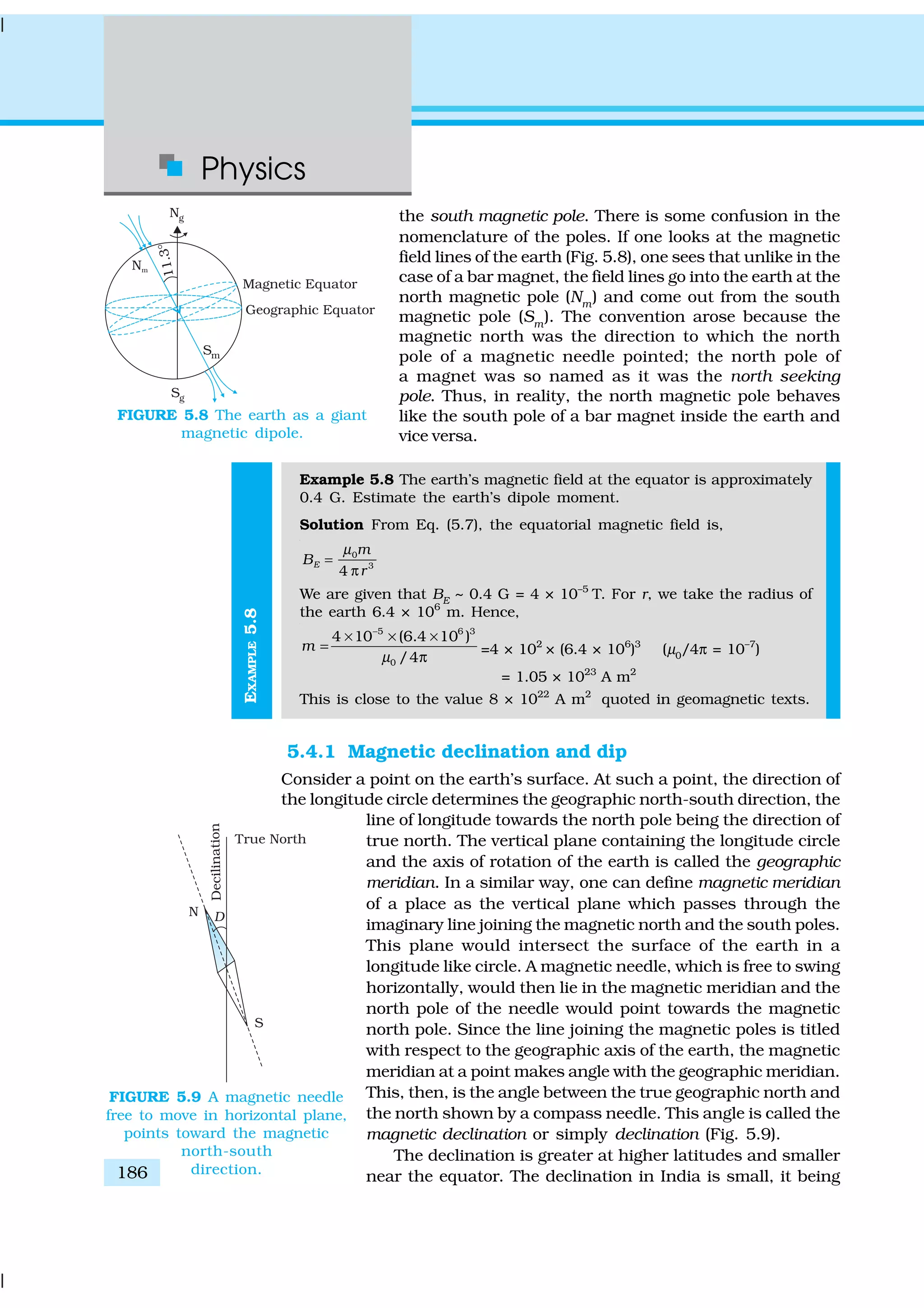
191. Magnetism and
Matter
187
0º41′ E at Delhi and 0º58′ W at Mumbai. Thus, at both these places a
magnetic needle shows the true north quite accurately.
There is one more quantity of interest. If a magnetic needle is perfectly
balanced about a horizontal axis so that it can swing in a plane of the
magnetic meridian, the needle would make an angle with the horizontal
(Fig. 5.10). This is known as the angle of dip (also known as inclination).
Thus, dip is the angle that the total magnetic field BE of the earth makes
with the surface of the earth. Figure 5.11 shows the magnetic meridian
plane at a point P on the surface of the earth. The plane is a section through
the earth. The total magnetic field at P
can be resolved into a horizontal
component HE
and a vertical
component ZE. The angle that BE makes
with HE
is the angle of dip, I.
In most of the northern hemisphere, the north pole of the dip needle
tilts downwards. Likewise in most of the southern hemisphere, the south
pole of the dip needle tilts downwards.
To describe the magnetic field of the earth at a point on its surface, we
need to specify three quantities, viz., the declination D, the angle of dip or
the inclination I and the horizontal component of the earth’s field HE
. These
are known as the element of the earth’s magnetic field.
Representing the verticle component by ZE, we have
ZE
= BE
sinI [5.10(a)]
HE
= BE
cosI [5.10(b)]
which gives,
tan E
E
Z
I
H
= [5.10(c)]
FIGURE 5.10 The circle is a
section through the earth
containing the magnetic
meridian. The angle between BE
and the horizontal component
HE
is the angle of dip.
FIGURE 5.11 The earth’s
magnetic field, BE
, its horizontal
and vertical components, HE
and
ZE
. Also shown are the
declination, D and the
inclination or angle of dip, I.

192. Physics
188
EXAMPLE5.9
WHAT HAPPENS TO MY COMPASS NEEDLES AT THE POLES?
A compass needle consists of a magnetic needle which floats on a pivotal point. When the
compass is held level, it points along the direction of the horizontal component of the earth’s
magnetic field at the location. Thus, the compass needle would stay along the magnetic
meridian of the place. In some places on the earth there are deposits of magnetic minerals
which cause the compass needle to deviate from the magnetic meridian. Knowing the magnetic
declination at a place allows us to correct the compass to determine the direction of true
north.
So what happens if we take our compass to the magnetic pole? At the poles, the magnetic
field lines are converging or diverging vertically so that the horizontal component is negligible.
If the needle is only capable of moving in a horizontal plane, it can point along any direction,
rendering it useless as a direction finder. What one needs in such a case is a dip needle
which is a compass pivoted to move in a vertical plane containing the magnetic field of the
earth. The needle of the compass then shows the angle which the magnetic field makes with
the vertical. At the magnetic poles such a needle will point straight down.
Example 5.9 In the magnetic meridian of a certain place, the
horizontal component of the earth’s magnetic field is 0.26G and the
dip angle is 60º. What is the magnetic field of the earth at this location?
Solution
It is given that HE
= 0.26 G. From Fig. 5.11, we have
0
cos60 E
E
H
B
=
0
cos60
E
E
H
B =
=
0.26
0.52G
(1/2)
=

193. Magnetism and
Matter
189
5.5 MAGNETISATION AND MAGNETIC INTENSITY
The earth abounds with a bewildering variety of elements and compounds.
In addition, we have been synthesising new alloys, compounds and even
elements. One would like to classify the magnetic properties of these
substances. In the present section, we define and explain certain terms
which will help us to carry out this exercise.
We have seen that a circulating electron in an atom has a magnetic
moment. In a bulk material, these moments add up vectorially and they
can give a net magnetic moment which is non-zero. We define
magnetisation M of a sample to be equal to its net magnetic moment per
unit volume:
net
V
=
m
M (5.11)
M is a vector with dimensions L–1
A and is measured in a units of A m–1
.
Consider a long solenoid of n turns per unit length and carrying a
current I. The magnetic field in the interior of the solenoid was shown to
be given by
EARTH’S MAGNETIC FIELD
It must not be assumed that there is a giant bar magnet deep inside the earth which is
causing the earth’s magnetic field. Although there are large deposits of iron inside the earth,
it is highly unlikely that a large solid block of iron stretches from the magnetic north pole to
the magnetic south pole. The earth’s core is very hot and molten, and the ions of iron and
nickel are responsible for earth’s magnetism. This hypothesis seems very probable. Moon,
which has no molten core, has no magnetic field, Venus has a slower rate of rotation, and a
weaker magnetic field, while Jupiter, which has the fastest rotation rate among planets, has
a fairly strong magnetic field. However, the precise mode of these circulating currents and
the energy needed to sustain them are not very well understood. These are several open
questions which form an important area of continuing research.
The variation of the earth’s magnetic field with position is also an interesting area of
study. Charged particles emitted by the sun flow towards the earth and beyond, in a stream
called the solar wind. Their motion is affected by the earth’s magnetic field, and in turn, they
affect the pattern of the earth’s magnetic field. The pattern of magnetic field near the poles is
quite different from that in other regions of the earth.
The variation of earth’s magnetic field with time is no less fascinating. There are short
term variations taking place over centuries and long term variations taking place over a
period of a million years. In a span of 240 years from 1580 to 1820 AD, over which records
are available, the magnetic declination at London has been found to change by 3.5º,
suggesting that the magnetic poles inside the earth change position with time. On the scale
of a million years, the earth’s magnetic fields has been found to reverse its direction. Basalt
contains iron, and basalt is emitted during volcanic activity. The little iron magnets inside it
align themselves parallel to the magnetic field at that place as the basalt cools and solidifies.
Geological studies of basalt containing such pieces of magnetised region have provided
evidence for the change of direction of earth’s magnetic field, several times in the past.

194. Physics
190
B0
= µ0
nI (5.12)
If the interior of the solenoid is filled with a material with non-zero
magnetisation, the field inside the solenoid will be greater than B0
. The
net B field in the interior of the solenoid may be expressed as
B = B0 + Bm (5.13)
where Bm
is the field contributed by the material core. It turns out that
this additional field Bm is proportional to the magnetisation M of the
material and is expressed as
Bm = µ0M (5.14)
where µ0
is the same constant (permeability of vacuum) that appears in
Biot-Savart’s law.
It is convenient to introduce another vector field H, called the magnetic
intensity, which is defined by
0
–
µ
=
B
H M (5.15)
where H has the same dimensions as M and is measured in units of A m–1
.
Thus, the total magnetic field B is written as
B = µ0
(H + M) (5.16)
We repeat our defining procedure. We have partitioned the contribution
to the total magnetic field inside the sample into two parts: one, due to
external factors such as the current in the solenoid. This is represented
by H. The other is due to the specific nature of the magnetic material,
namely M. The latter quantity can be influenced by external factors. This
influence is mathematically expressed as
χ=M H (5.17)
where χ, a dimensionless quantity, is appropriately called the magnetic
susceptibility. It is a measure of how a magnetic material responds to an
external field. Table 5.2 lists χ for some elements. It is small and positive
for materials, which are called paramagnetic. It is small and negative for
materials, which are termed diamagnetic. In the latter case M and H are
opposite in direction. From Eqs. (5.16) and (5.17) we obtain,
0(1 )µ χ= +B H (5.18)
= µ0
µr
H
= µ H (5.19)
where µr
= 1 + χ, is a dimensionless quantity called the relative magnetic
permeability of the substance. It is the analog of the dielectric constant in
electrostatics. The magnetic permeability of the substance is µ and it has
the same dimensions and units as µ0
;
µ = µ0
µr
= µ0
(1+χ).
The three quantities χ, µr
and µ are interrelated and only one of
them is independent. Given one, the other two may be easily determined.

195. Magnetism and
Matter
191
EXAMPLE5.10
Example 5.10 A solenoid has a core of a material with relative
permeability 400. The windings of the solenoid are insulated from the
core and carry a current of 2A. If the number of turns is 1000 per
metre, calculate (a) H, (b) M, (c) B and (d) the magnetising current Im
.
Solution
(a) The field H is dependent of the material of the core, and is
H = nI = 1000 × 2.0 = 2 ×103
A/m.
(b) The magnetic field B is given by
B = µr
µ0
H
= 400 × 4π ×10–7
(N/A2
) × 2 × 103
(A/m)
= 1.0 T
(c) Magnetisation is given by
M = (B– µ0
H)/ µ0
= (µr
µ0
H–µ0
H)/µ0
= (µr
– 1)H = 399 × H
≅ 8 × 105
A/m
(d) The magnetising current IM
is the additional current that needs
to be passed through the windings of the solenoid in the absence
of the core which would give a B value as in the presence of the
core. Thus B = µr
n0
(I + IM
). Using I = 2A, B = 1 T, we get IM
= 794 A.
5.6 MAGNETIC PROPERTIES OF MATERIALS
The discussion in the previous section helps us to classify materials as
diamagnetic, paramagnetic or ferromagnetic. In terms of the susceptibility
χ , a material is diamagnetic if χ is negative, para- if χ is positive and
small, and ferro- if χ is large and positive.
A glance at Table 5.3 gives one a better feeling for these
materials. Here ε is a small positive number introduced to quantify
paramagnetic materials. Next, we describe these materials in some
detail.
TABLE 5.2 MAGNETIC SUSCEPTIBILITY OF SOME ELEMENTS AT 300 K
Diamagnetic substance χχ Paramagnetic substance χχ
Bismuth –1.66 × 10–5
Aluminium 2.3 × 10–5
Copper –9.8 × 10–6
Calcium 1.9 × 10–5
Diamond –2.2 × 10–5
Chromium 2.7 × 10–4
Gold –3.6 × 10–5
Lithium 2.1 × 10–5
Lead –1.7 × 10–5
Magnesium 1.2 × 10–5
Mercury –2.9 × 10–5
Niobium 2.6 × 10–5
Nitrogen (STP) –5.0 × 10–9
Oxygen (STP) 2.1 × 10–6
Silver –2.6 × 10–5
Platinum 2.9 × 10–4
Silicon –4.2 × 10–6
Tungsten 6.8 × 10–5

196. Physics
192
5.6.1 Diamagnetism
Diamagnetic substances are those which have tendency to move from
stronger to the weaker part of the external magnetic field. In other words,
unlike the way a magnet attracts metals like iron, it would repel a
diamagnetic substance.
Figure 5.12(a) shows a bar of diamagnetic material placed in an external
magnetic field. The field lines are repelled or expelled and the field inside
the material is reduced. In most cases, as is evident from
Table 5.2, this reduction is slight, being one part in 105
. When placed in a
non-uniform magnetic field, the bar will tend to move from high to low field.
The simplest explanation for diamagnetism is as follows. Electrons in
an atom orbiting around nucleus possess orbital angular momentum.
These orbiting electrons are equivalent to current-carrying loop and thus
possess orbital magnetic moment. Diamagnetic substances are the ones
in which resultant magnetic moment in an atom is zero. When magnetic
field is applied, those electrons having orbital magnetic moment in the
same direction slow down and those in the opposite direction speed up.
This happens due to induced current in accordance with Lenz’s law which
you will study in Chapter 6. Thus, the substance develops a net magnetic
moment in direction opposite to that of the applied field and hence
repulsion.
Some diamagnetic materials are bismuth, copper, lead, silicon,
nitrogen (at STP), water and sodium chloride. Diamagnetism is present
in all the substances. However, the effect is so weak in most cases that it
gets shifted by other effects like paramagnetism, ferromagnetism, etc.
The most exotic diamagnetic materials are superconductors. These
are metals, cooled to very low temperatures which exhibits both perfect
conductivity and perfect diamagnetism. Here the field lines are completely
expelled! χ = –1 and µr
= 0. A superconductor repels a magnet and (by
Newton’s third law) is repelled by the magnet. The phenomenon of perfect
diamagnetism in superconductors is called the Meissner effect, after the
name of its discoverer. Superconducting magnets can be gainfully
exploited in variety of situations, for example, for running magnetically
levitated superfast trains.
5.6.2 Paramagnetism
Paramagnetic substances are those which get weakly magnetised when
placed in an external magnetic field. They have tendency to move from a
region of weak magnetic field to strong magnetic field, i.e., they get weakly
attracted to a magnet.
TABLE 5.3
Diamagnetic Paramagnetic Ferromagnetic
–1 ≤ χ < 0 0 < χ < ε χ >> 1
0 ≤ µr < 1 1< µr < 1+ ε µr >> 1
µ < µ0 µ > µ0 µ >> µ0
FIGURE 5.12
Behaviour of
magnetic field lines
near a
(a) diamagnetic,
(b) paramagnetic
substance.

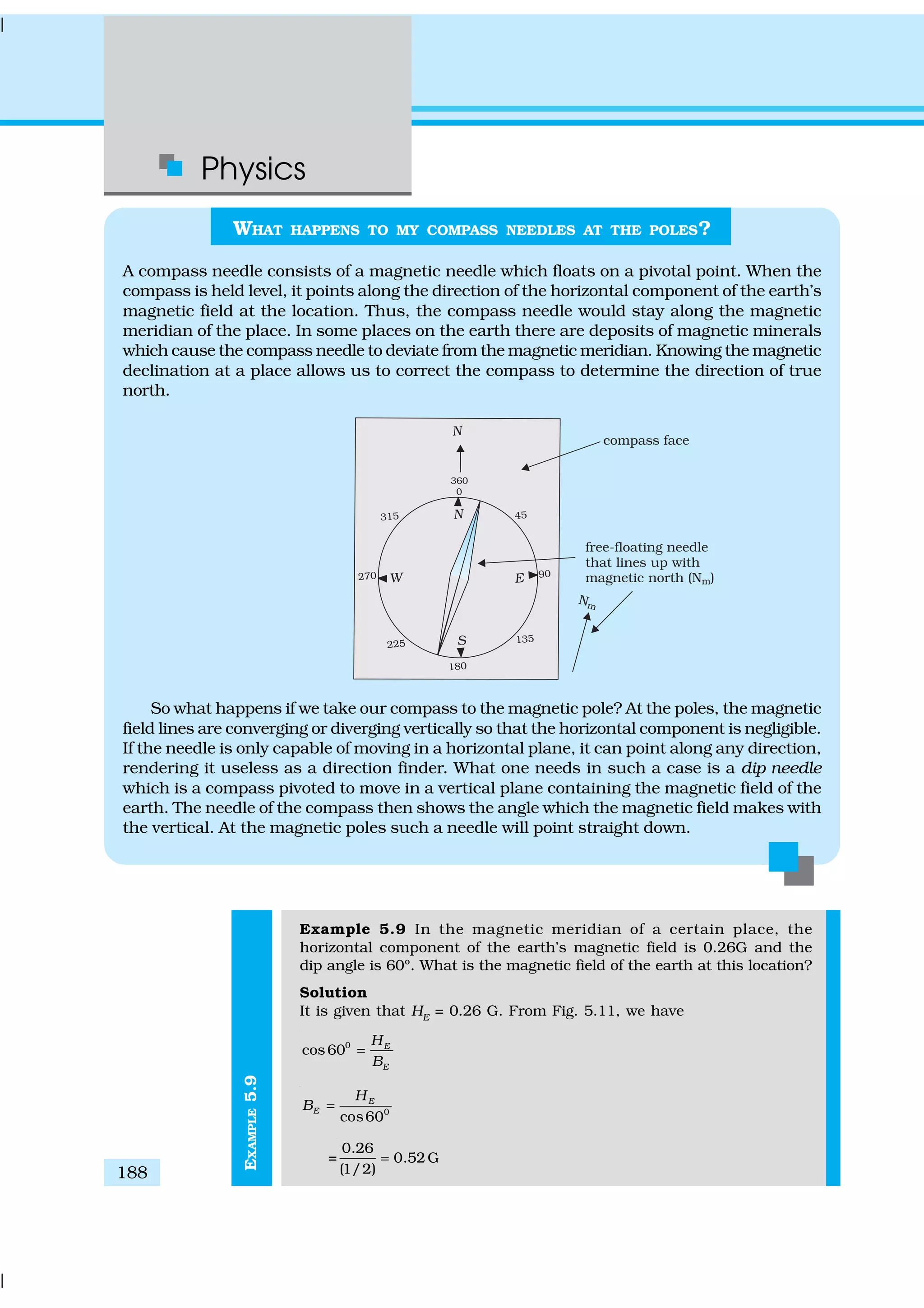
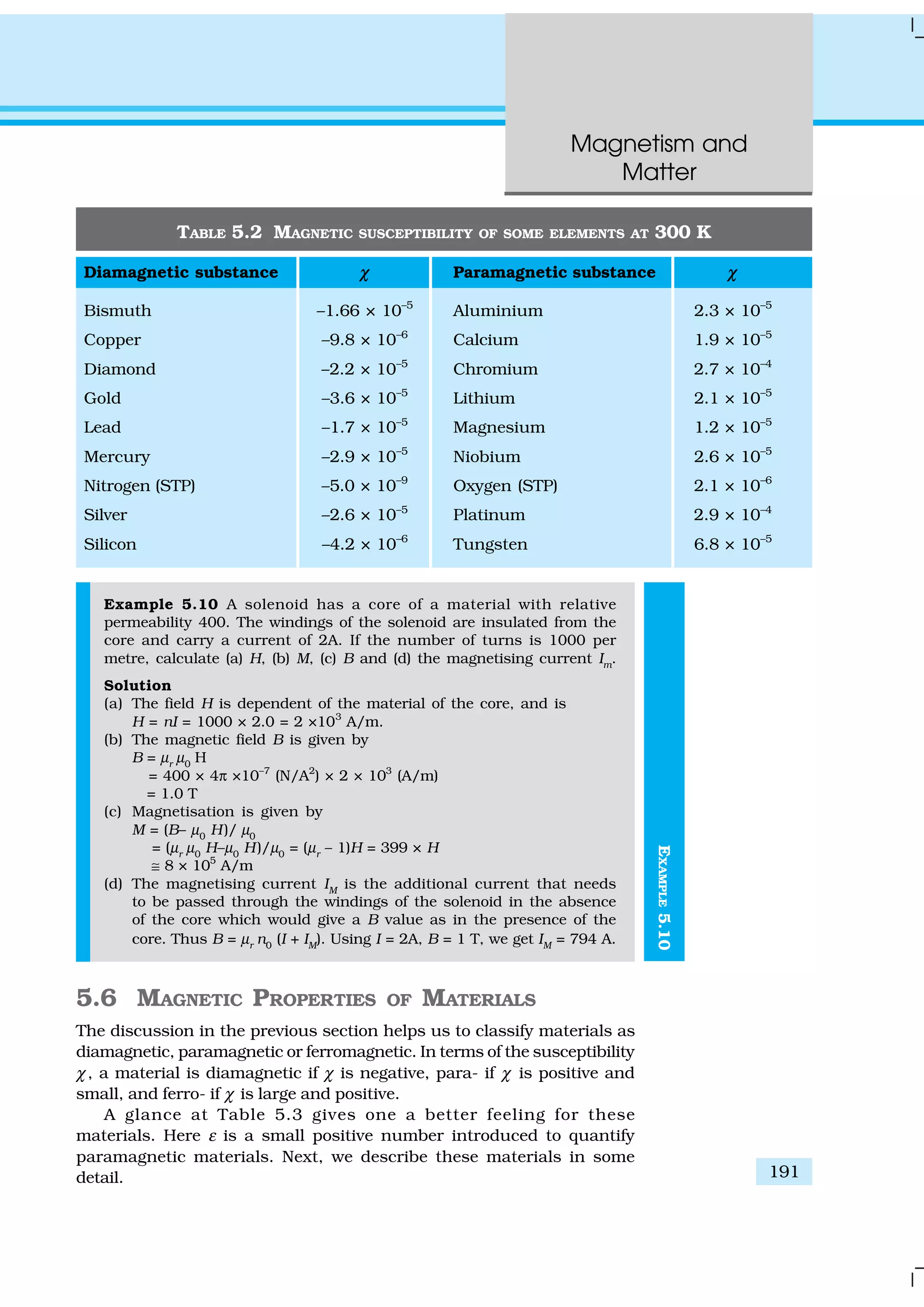
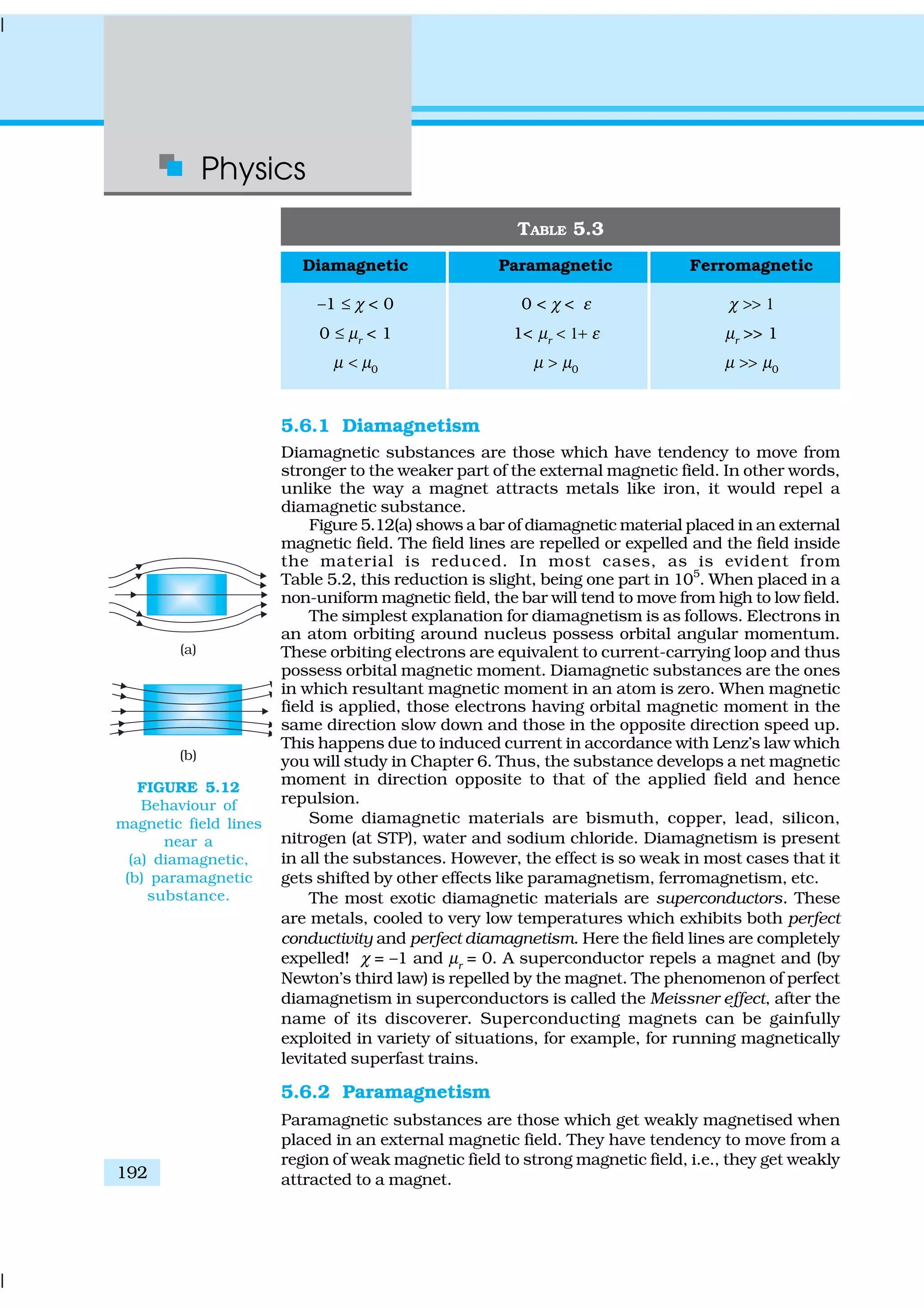
197. Magnetism and
Matter
193
The individual atoms (or ions or molecules) of a paramagnetic material
possess a permanent magnetic dipole moment of their own. On account
of the ceaseless random thermal motion of the atoms, no net magnetisation
is seen. In the presence of an external field B0
, which is strong enough,
and at low temperatures, the individual atomic dipole moment can be
made to align and point in the same direction as B0. Figure 5.12(b) shows
a bar of paramagnetic material placed in an external field. The field lines
gets concentrated inside the material, and the field inside is enhanced. In
most cases, as is evident from Table 5.2, this enhancement is slight, being
one part in 105
. When placed in a non-uniform magnetic field, the bar
will tend to move from weak field to strong.
Some paramagnetic materials are aluminium, sodium, calcium,
oxygen (at STP) and copper chloride. Experimentally, one finds that the
magnetisation of a paramagnetic material is inversely proportional to the
absolute temperature T,
0B
M C
T
= [5.20(a)]
or equivalently, using Eqs. (5.12) and (5.17)
0
C
T
µ
χ = [5.20(b)]
This is known as Curie’s law, after its discoverer Pieree Curie (1859-
1906). The constant C is called Curie’s constant. Thus, for a paramagnetic
material both χ and µr depend not only on the material, but also
(in a simple fashion) on the sample temperature. As the field is
increased or the temperature is lowered, the magnetisation increases until
it reaches the saturation value Ms, at which point all the dipoles are
perfectly aligned with the field. Beyond this, Curie’s law [Eq. (5.20)] is no
longer valid.
5.6.3 Ferromagnetism
Ferromagnetic substances are those which gets strongly magnetised when
placed in an external magnetic field. They have strong tendency to move
from a region of weak magnetic field to strong magnetic field, i.e., they get
strongly attracted to a magnet.
The individual atoms (or ions or molecules) in a ferromagnetic material
possess a dipole moment as in a paramagnetic material. However, they
interact with one another in such a way that they spontaneously align
themselves in a common direction over a macroscopic volume called
domain. The explanation of this cooperative effect requires quantum
mechanics and is beyond the scope of this textbook. Each domain has a
net magnetisation. Typical domain size is 1mm and the domain contains
about 1011
atoms. In the first instant, the magnetisation varies randomly
from domain to domain and there is no bulk magnetisation. This is shown
in Fig. 5.13(a). When we apply an external magnetic field B0
, the domains
orient themselves in the direction of B0 and simultaneously the domain
oriented in the direction of B0
grow in size. This existence of domains and
their motion in B0
are not speculations. One may observe this under a
microscope after sprinkling a liquid suspension of powdered
FIGURE 5.13
(a) Randomly
oriented domains,
(b) Aligned domains.
Magneticmaterials,domain,etc.:
http://www.aacg.bham.ac.uk/magnetic_materials/

198. Physics
194
EXAMPLE5.11
ferromagnetic substance of samples. This motion of suspension can be
observed. Figure 5.12(b) shows the situation when the domains have
aligned and amalgamated to form a single ‘giant’ domain.
Thus, in a ferromagnetic material the field lines are highly
concentrated. In non-uniform magnetic field, the sample tends to move
towards the region of high field. We may wonder as to what happens
when the external field is removed. In some ferromagnetic materials the
magnetisation persists. Such materials are called hard magnetic materials
or hard ferromagnets. Alnico, an alloy of iron, aluminium, nickel, cobalt
and copper, is one such material. The naturally occurring lodestone is
another. Such materials form permanent magnets to be used among other
things as a compass needle. On the other hand, there is a class of
ferromagnetic materials in which the magnetisation disappears on removal
of the external field. Soft iron is one such material. Appropriately enough,
such materials are called soft ferromagnetic materials. There are a number
of elements, which are ferromagnetic: iron, cobalt, nickel, gadolinium,
etc. The relative magnetic permeability is >1000!
The ferromagnetic property depends on temperature. At high enough
temperature, a ferromagnet becomes a paramagnet. The domain structure
disintegrates with temperature. This disappearance of magnetisation with
temperature is gradual. It is a phase transition reminding us of the melting
of a solid crystal. The temperature of transition from ferromagnetic to
paramagnetism is called the Curie temperature Tc
. Table 5.4 lists
the Curie temperature of certain ferromagnets. The susceptibility
above the Curie temperature, i.e., in the paramagnetic phase is
described by,
( )c
c
C
T T
T T
χ = >
−
(5.21)
TABLE 5.4 CURIE TEMPERATURE TC
OF SOME
FERROMAGNETIC MATERIALS
Material Tc (K)
Cobalt 1394
Iron 1043
Fe2
O3
893
Nickel 631
Gadolinium 317
Example 5.11 A domain in ferromagnetic iron is in the form of a cube
of side length 1µm. Estimate the number of iron atoms in the domain
and the maximum possible dipole moment and magnetisation of the
domain. The molecular mass of iron is 55 g/mole and its density
is 7.9 g/cm3
. Assume that each iron atom has a dipole moment
of 9.27×10–24
A m2
.
Hysterisisinmagneticmaterials:
http://hyperphysics.phy-astr.gsu.edu/hbase/solids/hyst.html

199. Magnetism and
Matter
195
EXAMPLE5.11
Solution The volume of the cubic domain is
V = (10–6
m)3
= 10–18
m3
= 10–12
cm3
Its mass is volume × density = 7.9 g cm–3
× 10–12
cm3
= 7.9 × 10–12
g
It is given that Avagadro number (6.023 × 1023
) of iron atoms have a
mass of 55 g. Hence, the number of atoms in the domain is
12 23
7.9 10 6.023 10
55
N
−
× × ×
=
= 8.65 × 1010
atoms
The maximum possible dipole moment mmax
is achieved for the
(unrealistic) case when all the atomic moments are perfectly aligned.
Thus,
mmax
= (8.65 × 1010
) × (9.27 × 10–24
)
= 8.0 × 10–13
A m2
The consequent magnetisation is
Mmax
= mmax
/Domain volume
= 8.0 × 10–13
Am2
/10–18
m3
= 8.0 × 105
Am–1
The relation between B and H in ferromagnetic materials is complex.
It is often not linear and it depends on the magnetic history of the sample.
Figure 5.14 depicts the behaviour of the material as we take it through
one cycle of magnetisation. Let the material be unmagnetised initially. We
place it in a solenoid and increase the current through the
solenoid. The magnetic field B in the material rises and
saturates as depicted in the curve Oa. This behaviour
represents the alignment and merger of domains until no
further enhancement is possible. It is pointless to increase
the current (and hence the magnetic intensity H) beyond
this. Next, we decrease H and reduce it to zero. At H = 0, B
≠ 0. This is represented by the curve ab. The value of B at
H = 0 is called retentivity or remanence. In Fig. 5.14, BR
~
1.2 T, where the subscript R denotes retentivity. The
domains are not completely randomised even though the
external driving field has been removed. Next, the current
in the solenoid is reversed and slowly increased. Certain
domains are flipped until the net field inside stands
nullified. This is represented by the curve bc. The value of
H at c is called coercivity. In Fig. 5.14 Hc
~ –90 A m–1
. As
the reversed current is increased in magnitude, we once
again obtain saturation. The curve cd depicts this. The
saturated magnetic field Bs
~ 1.5 T. Next, the current is
reduced (curve de) and reversed (curve ea). The cycle repeats
itself. Note that the curve Oa does not retrace itself as H is reduced. For a
given value of H, B is not unique but depends on previous history of the
sample. This phenomenon is called hysterisis. The word hysterisis means
lagging behind (and not ‘history’).
5.7 PERMANENT MAGNETS AND ELECTROMAGNETS
Substances which at room temperature retain their ferromagnetic property
for a long period of time are called permanent magnets. Permanent
FIGURE 5.14 The magnetic
hysteresis loop is the B-H curve for
ferromagnetic materials.

200. Physics
196
magnets can be made in a variety of ways. One can hold an
iron rod in the north-south direction and hammer it repeatedly.
The method is illustrated in Fig. 5.15. The illustration is from
a 400 year old book to emphasise that the making of
permanent magnets is an old art. One can also hold a steel
rod and stroke it with one end of a bar magnet a large number
of times, always in the same sense to make a permanent
magnet.
An efficient way to make a permanent magnet is to place a
ferromagnetic rod in a solenoid and pass a current. The
magnetic field of the solenoid magnetises the rod.
The hysteresis curve (Fig. 5.14) allows us to select suitable
materials for permanent magnets. The material should have
high retentivity so that the magnet is strong and high coercivity
so that the magnetisation is not erased by stray magnetic fields,
temperature fluctuations or minor mechanical damage.
Further, the material should have a high permeability. Steel is
one-favoured choice. It has a slightly smaller retentivity than
soft iron but this is outweighed by the much smaller coercivity
of soft iron. Other suitable materials for permanent magnets
are alnico, cobalt steel and ticonal.
Core of electromagnets are made of ferromagnetic materials
which have high permeability and low retentivity. Soft iron is a suitable
material for electromagnets. On placing a soft iron rod in a solenoid and
passing a current, we increase the magnetism of the solenoid by a
thousand fold. When we switch off the solenoid current, the magnetism is
effectively switched off since the soft iron core has a low retentivity. The
arrangement is shown in Fig. 5.16.
FIGURE 5.15 A blacksmith
forging a permanent magnet by
striking a red-hot rod of iron
kept in the north-south
direction with a hammer. The
sketch is recreated from an
illustration in De Magnete, a
work published in 1600 and
authored by William Gilbert,
the court physician to Queen
Elizabeth of England.
FIGURE 5.16 A soft iron core in solenoid acts as an electromagnet.
In certain applications, the material goes through an ac cycle of
magnetisation for a long period. This is the case in transformer cores and
telephone diaphragms. The hysteresis curve of such materials must be
narrow. The energy dissipated and the heating will consequently be small.
The material must have a high resistivity to lower eddy current losses.
You will study about eddy currents in Chapter 6.
Electromagnets are used in electric bells, loudspeakers and telephone
diaphragms. Giant electromagnets are used in cranes to lift machinery,
and bulk quantities of iron and steel.
IndiaísMagneticField:
http://iigs.iigm.res.in

201. Magnetism and
Matter
197
SUMMARY
1. The science of magnetism is old. It has been known since ancient times
that magnetic materials tend to point in the north-south direction; like
magnetic poles repel and unlike ones attract; and cutting a bar magnet
in two leads to two smaller magnets. Magnetic poles cannot be isolated.
2. When a bar magnet of dipole moment m is placed in a uniform magnetic
field B,
(a) the force on it is zero,
(b) the torque on it is m × B,
(c) its potential energy is –m.B, where we choose the zero of energy at
the orientation when m is perpendicular to B.
3. Consider a bar magnet of size l and magnetic moment m, at a distance
r from its mid-point, where r >>l, the magnetic field B due to this bar
is,
0
3
2 r
µ
=
π
m
B (along axis)
= 0
3
–
4 r
µ
π
m
(along equator)
4. Gauss’s law for magnetism states that the net magnetic flux through
any closed surface is zero
0B
all area
elements
φ
∆
= ∆ =∑
S
B Sg
5. The earth’s magnetic field resembles that of a (hypothetical) magnetic
dipole located at the centre of the earth. The pole near the geographic
north pole of the earth is called the north magnetic pole. Similarly, the
pole near the geographic south pole is called the south magnetic pole.
This dipole is aligned making a small angle with the rotation axis of
the earth. The magnitude of the field on the earth’s surface ≈ 4 × 10–5
T.
MAPPING INDIA’S MAGNETIC FIELD
Because of its practical application in prospecting, communication, and navigation, the
magnetic field of the earth is mapped by most nations with an accuracy comparable to
geographical mapping. In India over a dozen observatories exist, extending from
Trivandrum (now Thrivuvananthapuram) in the south to Gulmarg in the north. These
observatories work under the aegis of the Indian Institute of Geomagnetism (IIG), in Colaba,
Mumbai. The IIG grew out of the Colaba and Alibag observatories and was formally
established in 1971. The IIG monitors (via its nation-wide observatories), the geomagnetic
fields and fluctuations on land, and under the ocean and in space. Its services are used
by the Oil and Natural Gas Corporation Ltd. (ONGC), the National Institute of
Oceanography (NIO) and the Indian Space Research Organisation (ISRO). It is a part of
the world-wide network which ceaselessly updates the geomagnetic data. Now India has
a permanent station called Gangotri.

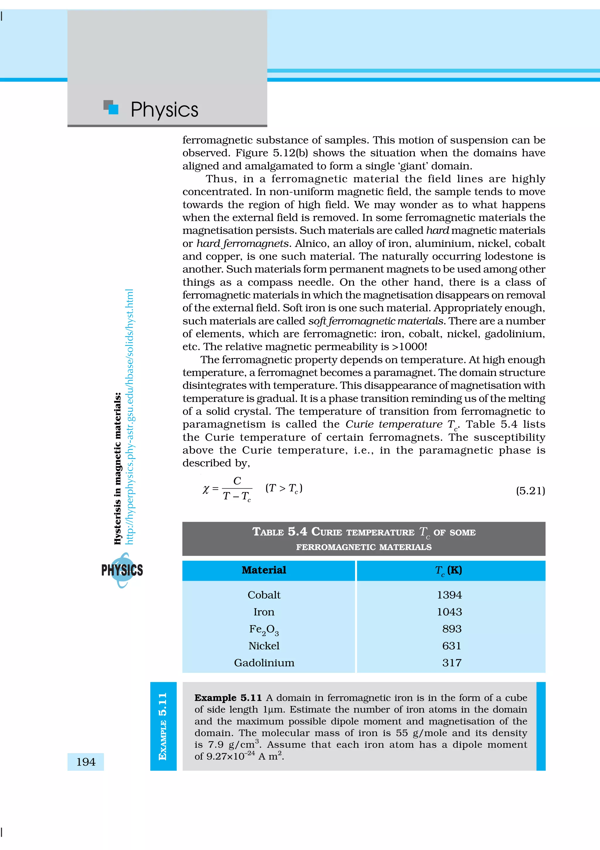
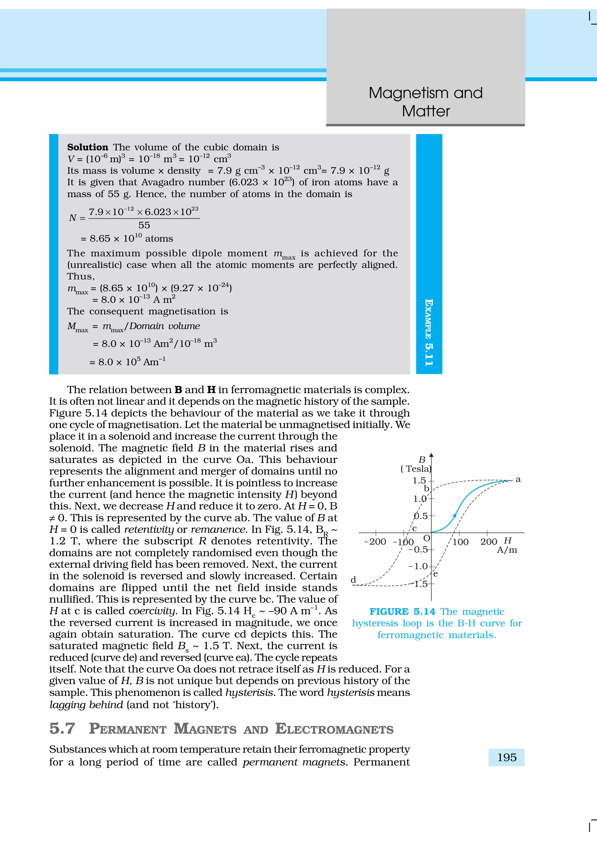
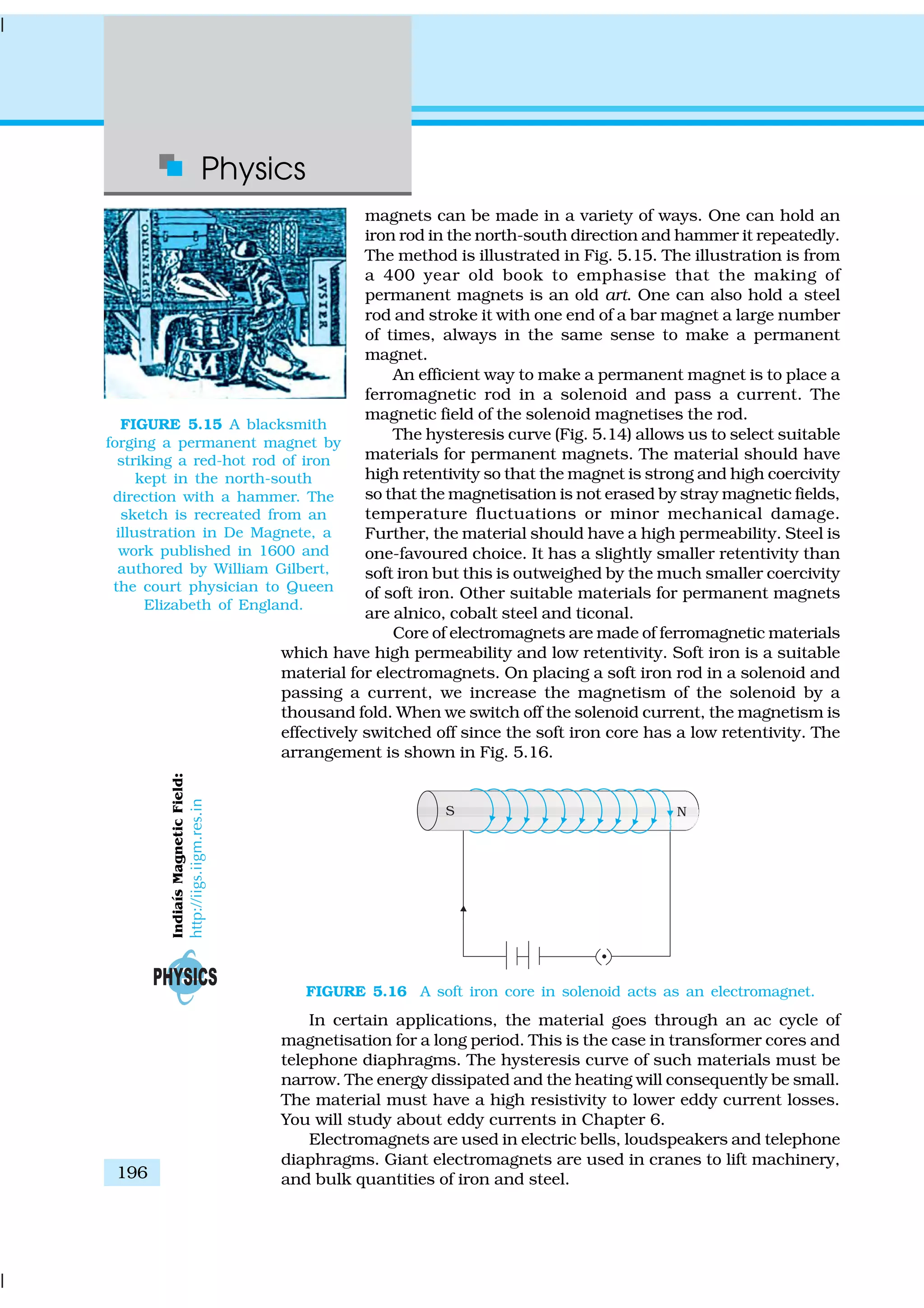
202. Physics
198
6. Three quantities are needed to specify the magnetic field of the earth
on its surface – the horizontal component, the magnetic declination,
and the magnetic dip. These are known as the elements of the earth’s
magnetic field.
7. Consider a material placed in an external magnetic field B0
. The
magnetic intensity is defined as,
0
0µ
=
B
H
The magnetisation M of the material is its dipole moment per unit volume.
The magnetic field B in the material is,
B = µ0 (H + M)
8. For a linear material M = χ H. So that B = µ H and χ is called the
magnetic susceptibility of the material. The three quantities, χ, the
relative magnetic permeability µr
, and the magnetic permeability µ are
related as follows:
µ = µ0
µr
µr = 1+ χ
9. Magnetic materials are broadly classified as: diamagnetic, paramagnetic,
and ferromagnetic. For diamagnetic materials χ is negative and small
and for paramagnetic materials it is positive and small. Ferromagnetic
materials have large χ and are characterised by non-linear relation
between B and H. They show the property of hysteresis.
10. Substances, which at room temperature, retain their ferromagnetic
property for a long period of time are called permanent magnets.
Physical quantity Symbol Nature Dimensions Units Remarks
Permeability of µ0
Scalar [MLT–2
A–2
] T m A–1
µ0
/4π = 10–7
free space
Magnetic field, B Vector [MT–2
A–1
] T (tesla) 104
G (gauss) = 1 T
Magnetic induction,
Magnetic flux density
Magnetic moment m Vector [L–2
A] A m2
Magnetic flux φB
Scalar [ML2
T–2
A–1
] W (weber) W = T m2
Magnetisation M Vector [L–1
A] A m–1
Magnetic moment
Volume
Magnetic intensity H Vector [L–1
A] A m–1
B = µ0
(H + M)
Magnetic field
strength
Magnetic χ Scalar - - M = χH
susceptibility
Relative magnetic µr
Scalar - - B = µ0
µr
H
permeability
Magnetic permeability µ Scalar [MLT–2
A–2
] T m A–1
µ = µ0
µr
N A–2
B = µ H

203. Magnetism and
Matter
199
POINTS TO PONDER
1. A satisfactory understanding of magnetic phenomenon in terms of moving
charges/currents was arrived at after 1800 AD. But technological
exploitation of the directional properties of magnets predates this scientific
understanding by two thousand years. Thus, scientific understanding is
not a necessary condition for engineering applications. Ideally, science
and engineering go hand-in-hand, one leading and assisting the other in
tandem.
2. Magnetic monopoles do not exist. If you slice a magnet in half, you get
two smaller magnets. On the other hand, isolated positive and negative
charges exist. There exists a smallest unit of charge, for example, the
electronic charge with value |e| = 1.6 ×10–19
C. All other charges are
integral multiples of this smallest unit charge. In other words, charge is
quantised. We do not know why magnetic monopoles do not exist or why
electric charge is quantised.
3. A consequence of the fact that magnetic monopoles do not exist is that
the magnetic field lines are continuous and form closed loops. In contrast,
the electrostatic lines of force begin on a positive charge and terminate
on the negative charge (or fade out at infinity).
4. The earth’s magnetic field is not due to a huge bar magnet inside it. The
earth’s core is hot and molten. Perhaps convective currents in this core
are responsible for the earth’s magnetic field. As to what ‘dynamo’ effect
sustains this current, and why the earth’s field reverses polarity every
million years or so, we do not know.
5. A miniscule difference in the value of χ, the magnetic susceptibility, yields
radically different behaviour: diamagnetic versus paramagnetic. For
diamagnetic materials χ = –10–5
whereas χ = +10–5
for paramagnetic
materials.
6. There exists a perfect diamagnet, namely, a superconductor. This is a
metal at very low temperatures. In this case χ = –1, µr
= 0, µ = 0. The
external magnetic field is totally expelled. Interestingly, this material is
also a perfect conductor. However, there exists no classical theory which
ties these two properties together. A quantum-mechanical theory by
Bardeen, Cooper, and Schrieffer (BCS theory) explains these effects. The
BCS theory was proposed in1957 and was eventually recognised by a Nobel
Prize in physics in 1970.
7. The phenomenon of magnetic hysteresis is reminiscent of similar
behaviour concerning the elastic properties of materials. Strain
may not be proportional to stress; here H and B (or M) are not
linearly related. The stress-strain curve exhibits hysteresis and
area enclosed by it represents the energy dissipated per unit volume.
A similar interpretation can be given to the B-H magnetic hysteresis
curve.
8. Diamagnetism is universal. It is present in all materials. But it
is weak and hard to detect if the substance is para- or ferromagnetic.
9. We have classified materials as diamagnetic, paramagnetic, and
ferromagnetic. However, there exist additional types of magnetic material
such as ferrimagnetic, anti-ferromagnetic, spin glass, etc. with properties
which are exotic and mysterious.

204. Physics
200
EXERCISES
5.1 Answer the following questions regarding earth’s magnetism:
(a) A vector needs three quantities for its specification. Name the
three independent quantities conventionally used to specify the
earth’s magnetic field.
(b) The angle of dip at a location in southern India is about 18º.
Would you expect a greater or smaller dip angle in Britain?
(c) If you made a map of magnetic field lines at Melbourne in
Australia, would the lines seem to go into the ground or come out
of the ground?
(d) In which direction would a compass free to move in the vertical
plane point to, if located right on the geomagnetic north or south
pole?
(e) The earth’s field, it is claimed, roughly approximates the field
due to a dipole of magnetic moment 8 × 1022
J T–1
located at its
centre. Check the order of magnitude of this number in some
way.
(f ) Geologists claim that besides the main magnetic N-S poles, there
are several local poles on the earth’s surface oriented in different
directions. How is such a thing possible at all?
5.2 Answer the following questions:
(a) The earth’s magnetic field varies from point to point in space.
Does it also change with time? If so, on what time scale does it
change appreciably?
(b) The earth’s core is known to contain iron. Yet geologists do not
regard this as a source of the earth’s magnetism. Why?
(c) The charged currents in the outer conducting regions of the
earth’s core are thought to be responsible for earth’s magnetism.
What might be the ‘battery’ (i.e., the source of energy) to sustain
these currents?
(d) The earth may have even reversed the direction of its field several
times during its history of 4 to 5 billion years. How can geologists
know about the earth’s field in such distant past?
(e) The earth’s field departs from its dipole shape substantially at
large distances (greater than about 30,000 km). What agencies
may be responsible for this distortion?
(f ) Interstellar space has an extremely weak magnetic field of the
order of 10–12
T. Can such a weak field be of any significant
consequence? Explain.
[Note: Exercise 5.2 is meant mainly to arouse your curiosity. Answers
to some questions above are tentative or unknown. Brief answers
wherever possible are given at the end. For details, you should consult
a good text on geomagnetism.]
5.3 A short bar magnet placed with its axis at 30º with a uniform external
magnetic field of 0.25 T experiences a torque of magnitude equal to
4.5 × 10–2
J. What is the magnitude of magnetic moment of the magnet?
5.4 A short bar magnet of magnetic moment m = 0.32 JT–1
is placed in a
uniform magnetic field of 0.15 T. If the bar is free to rotate in the
plane of the field, which orientation would correspond to its (a) stable,
and (b) unstable equilibrium? What is the potential energy of the
magnet in each case?

205. Magnetism and
Matter
201
5.5 A closely wound solenoid of 800 turns and area of cross section
2.5 × 10–4
m2
carries a current of 3.0 A. Explain the sense in which
the solenoid acts like a bar magnet. What is its associated magnetic
moment?
5.6 If the solenoid in Exercise 5.5 is free to turn about the vertical
direction and a uniform horizontal magnetic field of 0.25 T is applied,
what is the magnitude of torque on the solenoid when its axis makes
an angle of 30° with the direction of applied field?
5.7 A bar magnet of magnetic moment 1.5 J T–1
lies aligned with the
direction of a uniform magnetic field of 0.22 T.
(a) What is the amount of work required by an external torque to
turn the magnet so as to align its magnetic moment: (i) normal
to the field direction, (ii) opposite to the field direction?
(b) What is the torque on the magnet in cases (i) and (ii)?
5.8 A closely wound solenoid of 2000 turns and area of cross-section
1.6 × 10–4
m2
, carrying a current of 4.0 A, is suspended through its
centre allowing it to turn in a horizontal plane.
(a) What is the magnetic moment associated with the solenoid?
(b) What is the force and torque on the solenoid if a uniform
horizontal magnetic field of 7.5 × 10–2
T is set up at an angle of
30º with the axis of the solenoid?
5.9 A circular coil of 16 turns and radius 10 cm carrying a current of
0.75 A rests with its plane normal to an external field of magnitude
5.0 × 10–2
T. The coil is free to turn about an axis in its plane
perpendicular to the field direction. When the coil is turned slightly
and released, it oscillates about its stable equilibrium with a
frequency of 2.0 s–1
. What is the moment of inertia of the coil about
its axis of rotation?
5.10 A magnetic needle free to rotate in a vertical plane parallel to the
magnetic meridian has its north tip pointing down at 22º with the
horizontal. The horizontal component of the earth’s magnetic field
at the place is known to be 0.35 G. Determine the magnitude of the
earth’s magnetic field at the place.
5.11 At a certain location in Africa, a compass points 12º west of the
geographic north. The north tip of the magnetic needle of a dip circle
placed in the plane of magnetic meridian points 60º above the
horizontal. The horizontal component of the earth’s field is measured
to be 0.16 G. Specify the direction and magnitude of the earth’s field
at the location.
5.12 A short bar magnet has a magnetic moment of 0.48 J T–1
. Give the
direction and magnitude of the magnetic field produced by the magnet
at a distance of 10 cm from the centre of the magnet on (a) the axis,
(b) the equatorial lines (normal bisector) of the magnet.
5.13 A short bar magnet placed in a horizontal plane has its axis aligned
along the magnetic north-south direction. Null points are found on
the axis of the magnet at 14 cm from the centre of the magnet. The
earth’s magnetic field at the place is 0.36 G and the angle of dip is
zero. What is the total magnetic field on the normal bisector of the
magnet at the same distance as the null–point (i.e., 14 cm) from the
centre of the magnet? (At null points, field due to a magnet is equal
and opposite to the horizontal component of earth’s magnetic field.)
5.14 If the bar magnet in exercise 5.13 is turned around by 180º, where
will the new null points be located?

206. Physics
202
5.15 A short bar magnet of magnetic moment 5.25 × 10–2
J T–1
is placed
with its axis perpendicular to the earth’s field direction. At what
distance from the centre of the magnet, the resultant field is inclined
at 45º with earth’s field on (a) its normal bisector and (b) its axis.
Magnitude of the earth’s field at the place is given to be 0.42 G.
Ignore the length of the magnet in comparison to the distances
involved.
ADDITIONAL EXERCISES
5.16 Answer the following questions:
(a) Why does a paramagnetic sample display greater magnetisation
(for the same magnetising field) when cooled?
(b) Why is diamagnetism, in contrast, almost independent of
temperature?
(c) If a toroid uses bismuth for its core, will the field in the core be
(slightly) greater or (slightly) less than when the core is empty?
(d) Is the permeability of a ferromagnetic material independent of
the magnetic field? If not, is it more for lower or higher fields?
(e) Magnetic field lines are always nearly normal to the surface of a
ferromagnet at every point. (This fact is analogous to the static
electric field lines being normal to the surface of a conductor at
every point.) Why?
(f ) Would the maximum possible magnetisation of a paramagnetic
sample be of the same order of magnitude as the magnetisation
of a ferromagnet?
5.17 Answer the following questions:
(a) Explain qualitatively on the basis of domain picture the
irreversibility in the magnetisation curve of a ferromagnet.
(b) The hysteresis loop of a soft iron piece has a much smaller area
than that of a carbon steel piece. If the material is to go through
repeated cycles of magnetisation, which piece will dissipate greater
heat energy?
(c) ‘A system displaying a hysteresis loop such as a ferromagnet, is
a device for storing memory?’ Explain the meaning of this
statement.
(d) What kind of ferromagnetic material is used for coating magnetic
tapes in a cassette player, or for building ‘memory stores’ in a
modern computer?
(e) A certain region of space is to be shielded from magnetic fields.
Suggest a method.
5.18 A long straight horizontal cable carries a current of 2.5 A in the
direction 10º south of west to 10º north of east. The magnetic meridian
of the place happens to be 10º west of the geographic meridian. The
earth’s magnetic field at the location is 0.33 G, and the angle of dip
is zero. Locate the line of neutral points (ignore the thickness of the
cable). (At neutral points, magnetic field due to a current-carrying
cable is equal and opposite to the horizontal component of earth’s
magnetic field.)
5.19 A telephone cable at a place has four long straight horizontal wires
carrying a current of 1.0 A in the same direction east to west. The

207. Magnetism and
Matter
203
earth’s magnetic field at the place is 0.39 G, and the angle of dip is
35º. The magnetic declination is nearly zero. What are the resultant
magnetic fields at points 4.0 cm below the cable?
5.20 A compass needle free to turn in a horizontal plane is placed at the
centre of circular coil of 30 turns and radius 12 cm. The coil is in a
vertical plane making an angle of 45º with the magnetic meridian.
When the current in the coil is 0.35 A, the needle points west to
east.
(a) Determine the horizontal component of the earth’s magnetic field
at the location.
(b) The current in the coil is reversed, and the coil is rotated about
its vertical axis by an angle of 90º in the anticlockwise sense
looking from above. Predict the direction of the needle. Take the
magnetic declination at the places to be zero.
5.21 A magnetic dipole is under the influence of two magnetic fields. The
angle between the field directions is 60º, and one of the fields has a
magnitude of 1.2 × 10–2
T. If the dipole comes to stable equilibrium at
an angle of 15º with this field, what is the magnitude of the other
field?
5.22 A monoenergetic (18 keV) electron beam initially in the horizontal
direction is subjected to a horizontal magnetic field of 0.04 G normal
to the initial direction. Estimate the up or down deflection of the
beam over a distance of 30 cm (me
= 9.11 × 10–19
C). [Note: Data in
this exercise are so chosen that the answer will give you an idea of
the effect of earth’s magnetic field on the motion of the electron beam
from the electron gun to the screen in a TV set.]
5.23 A sample of paramagnetic salt contains 2.0 × 1024
atomic dipoles
each of dipole moment 1.5 × 10–23
J T–1
. The sample is placed under
a homogeneous magnetic field of 0.64 T, and cooled to a temperature
of 4.2 K. The degree of magnetic saturation achieved is equal to 15%.
What is the total dipole moment of the sample for a magnetic field of
0.98 T and a temperature of 2.8 K? (Assume Curie’s law)
5.24 A Rowland ring of mean radius 15 cm has 3500 turns of wire wound
on a ferromagnetic core of relative permeability 800. What is the
magnetic field B in the core for a magnetising current of 1.2 A?
5.25 The magnetic moment vectors µs
and µµl
associated with the intrinsic
spin angular momentum S and orbital angular momentum l,
respectively, of an electron are predicted by quantum theory (and
verified experimentally to a high accuracy) to be given by:
µs
= –(e/m) S,
µµl
= –(e/2m)l
Which of these relations is in accordance with the result expected
classically? Outline the derivation of the classical result.

208. 6.1 INTRODUCTION
Electricity and magnetism were considered separate and unrelated
phenomena for a long time. In the early decades of the nineteenth century,
experiments on electric current by Oersted, Ampere and a few others
established the fact that electricity and magnetism are inter-related. They
found that moving electric charges produce magnetic fields. For example,
an electric current deflects a magnetic compass needle placed in its vicinity.
This naturally raises the questions like: Is the converse effect possible?
Can moving magnets produce electric currents? Does the nature permit
such a relation between electricity and magnetism? The answer is
resounding yes! The experiments of Michael Faraday in England and
Joseph Henry in USA, conducted around 1830, demonstrated
conclusively that electric currents were induced in closed coils when
subjected to changing magnetic fields. In this chapter, we will study the
phenomena associated with changing magnetic fields and understand
the underlying principles. The phenomenon in which electric current is
generated by varying magnetic fields is appropriately called
electromagnetic induction.
When Faraday first made public his discovery that relative motion
between a bar magnet and a wire loop produced a small current in the
latter, he was asked, “What is the use of it?” His reply was: “What is the
use of a new born baby?” The phenomenon of electromagnetic induction
Chapter Six
ELECTROMAGNETIC
INDUCTION

209. Electromagnetic
Induction
205
is not merely of theoretical or academic interest but also
of practical utility. Imagine a world where there is no
electricity – no electric lights, no trains, no telephones and
no personal computers. The pioneering experiments of
Faraday and Henry have led directly to the development
of modern day generators and transformers. Today’s
civilisation owes its progress to a great extent to the
discovery of electromagnetic induction.
6.2 THE EXPERIMENTS OF FARADAY AND
HENRY
The discovery and understanding of electromagnetic
induction are based on a long series of experiments carried
out by Faraday and Henry. We shall now describe some
of these experiments.
Experiment6.1
Figure 6.1 shows a coil C1
* connected to a galvanometer
G. When the North-pole of a bar magnet is pushed
towards the coil, the pointer in the galvanometer deflects,
indicating the presence of electric current in the coil. The
deflection lasts as long as the bar magnet is in motion.
The galvanometer does not show any deflection when the
magnet is held stationary. When the magnet is pulled
away from the coil, the galvanometer shows deflection in
the opposite direction, which indicates reversal of the
current’s direction. Moreover, when the South-pole of
the bar magnet is moved towards or away from the
coil, the deflections in the galvanometer are opposite
to that observed with the North-pole for similar
movements. Further, the deflection (and hence current)
is found to be larger when the magnet is pushed
towards or pulled away from the coil faster. Instead,
when the bar magnet is held fixed and the coil C1
is
moved towards or away from the magnet, the same
effects are observed. It shows that it is the relative
motion between the magnet and the coil that is
responsible for generation (induction) of electric
current in the coil.
Experiment6.2
In Fig. 6.2 the bar magnet is replaced by a second coil
C2
connected to a battery. The steady current in the
coil C2
produces a steady magnetic field. As coil C2
is
* Wherever the term ‘coil or ‘loop’ is used, it is assumed that they are made up of
conducting material and are prepared using wires which are coated with insulating
material.
FIGURE 6.1 When the bar magnet is
pushed towards the coil, the pointer in
the galvanometer G deflects.
Josheph Henry [1797 –
1878] American experimental
physicist professor at
Princeton University and first
director of the Smithsonian
Institution. He made important
improvements in electro-
magnets by winding coils of
insulated wire around iron
pole pieces and invented an
electromagnetic motor and a
new, efficient telegraph. He
discoverd self-induction and
investigated how currents in
one circuit induce currents in
another.
JOSEPHHENRY(1797–1878)

210. Physics
206
moved towards the coil C1
, the galvanometer shows a
deflection. This indicates that electric current is induced in
coil C1
. When C2
is moved away, the galvanometer shows a
deflection again, but this time in the opposite direction. The
deflection lasts as long as coil C2
is in motion. When the coil
C2
is held fixed and C1
is moved, the same effects are observed.
Again, it is the relative motion between the coils that induces
the electric current.
Experiment6.3
The above two experiments involved relative motion between
a magnet and a coil and between two coils, respectively.
Through another experiment, Faraday showed that this
relative motion is not an absolute requirement. Figure 6.3
shows two coils C1
and C2
held stationary. Coil C1
is connected
to galvanometer G while the second coil C2
is connected to a
battery through a tapping key K.
FIGURE 6.2 Current is
induced in coil C1
due to motion
of the current carrying coil C2
.
FIGURE 6.3 Experimental set-up for Experiment 6.3.
It is observed that the galvanometer shows a momentary deflection
when the tapping key K is pressed. The pointer in the galvanometer returns
to zero immediately. If the key is held pressed continuously, there is no
deflection in the galvanometer. When the key is released, a momentory
deflection is observed again, but in the opposite direction. It is also observed
that the deflection increases dramatically when an iron rod is inserted
into the coils along their axis.
6.3 MAGNETIC FLUX
Faraday’s great insight lay in discovering a simple mathematical relation
to explain the series of experiments he carried out on electromagnetic
induction. However, before we state and appreciate his laws, we must get
familiar with the notion of magnetic flux, Φ B
. Magnetic flux is defined in
the same way as electric flux is defined in Chapter 1. Magnetic flux through
InteractiveanimationonFaraday’sexperimentsandLenz’slaw:
http://micro.magnet.fsu.edu/electromagnet/java/faraday/index.html

211. Electromagnetic
Induction
207
a plane of area A placed in a uniform magnetic field B (Fig. 6.4) can
be written as
Φ B
= B . A = BA cos θ (6.1)
where θ is angle between B and A. The notion of the area as a vector
has been discussed earlier in Chapter 1. Equation (6.1) can be
extended to curved surfaces and nonuniform fields.
If the magnetic field has different magnitudes and directions at
various parts of a surface as shown in Fig. 6.5, then the magnetic
flux through the surface is given by
1 1 2 2
d dB
Φ = + +B A B Ai i ... =
all
di i∑B Ai (6.2)
where ‘all’ stands for summation over all the area elements dAi
comprising the surface and Bi
is the magnetic field at the area element
dAi
. The SI unit of magnetic flux is weber (Wb) or tesla meter
squared (T m2
). Magnetic flux is a scalar quantity.
6.4 FARADAY’S LAW OF INDUCTION
From the experimental observations, Faraday arrived at a
conclusion that an emf is induced in a coil when magnetic flux
through the coil changes with time. Experimental observations
discussed in Section 6.2 can be explained using this concept.
The motion of a magnet towards or away from coil C1
in
Experiment 6.1 and moving a current-carrying coil C2
towards
or away from coil C1
in Experiment 6.2, change the magnetic
flux associated with coil C1
. The change in magnetic flux induces
emf in coil C1
. It was this induced emf which caused electric
current to flow in coil C1
and through the galvanometer. A
plausible explanation for the observations of Experiment 6.3 is
as follows: When the tapping key K is pressed, the current in
coil C2
(and the resulting magnetic field) rises from zero to a
maximum value in a short time. Consequently, the magnetic
flux through the neighbouring coil C1
also increases. It is the change in
magnetic flux through coil C1
that produces an induced emf in coil C1
.
When the key is held pressed, current in coil C2
is constant. Therefore,
there is no change in the magnetic flux through coil C1
and the current in
coil C1
drops to zero. When the key is released, the current in C2
and the
resulting magnetic field decreases from the maximum value to zero in a
short time. This results in a decrease in magnetic flux through coil C1
and hence again induces an electric current in coil C1
*. The common
point in all these observations is that the time rate of change of magnetic
flux through a circuit induces emf in it. Faraday stated experimental
observations in the form of a law called Faraday’s law of electromagnetic
induction. The law is stated below.
FIGURE 6.4 A plane of
surface area A placed in a
uniform magnetic field B.
FIGURE 6.5 Magnetic field Bi
at the ith
area element. dAi
represents area vector of the
ith
area element.
* Note that sensitive electrical instruments in the vicinity of an electromagnet
can be damaged due to the induced emfs (and the resulting currents) when the
electromagnet is turned on or off.

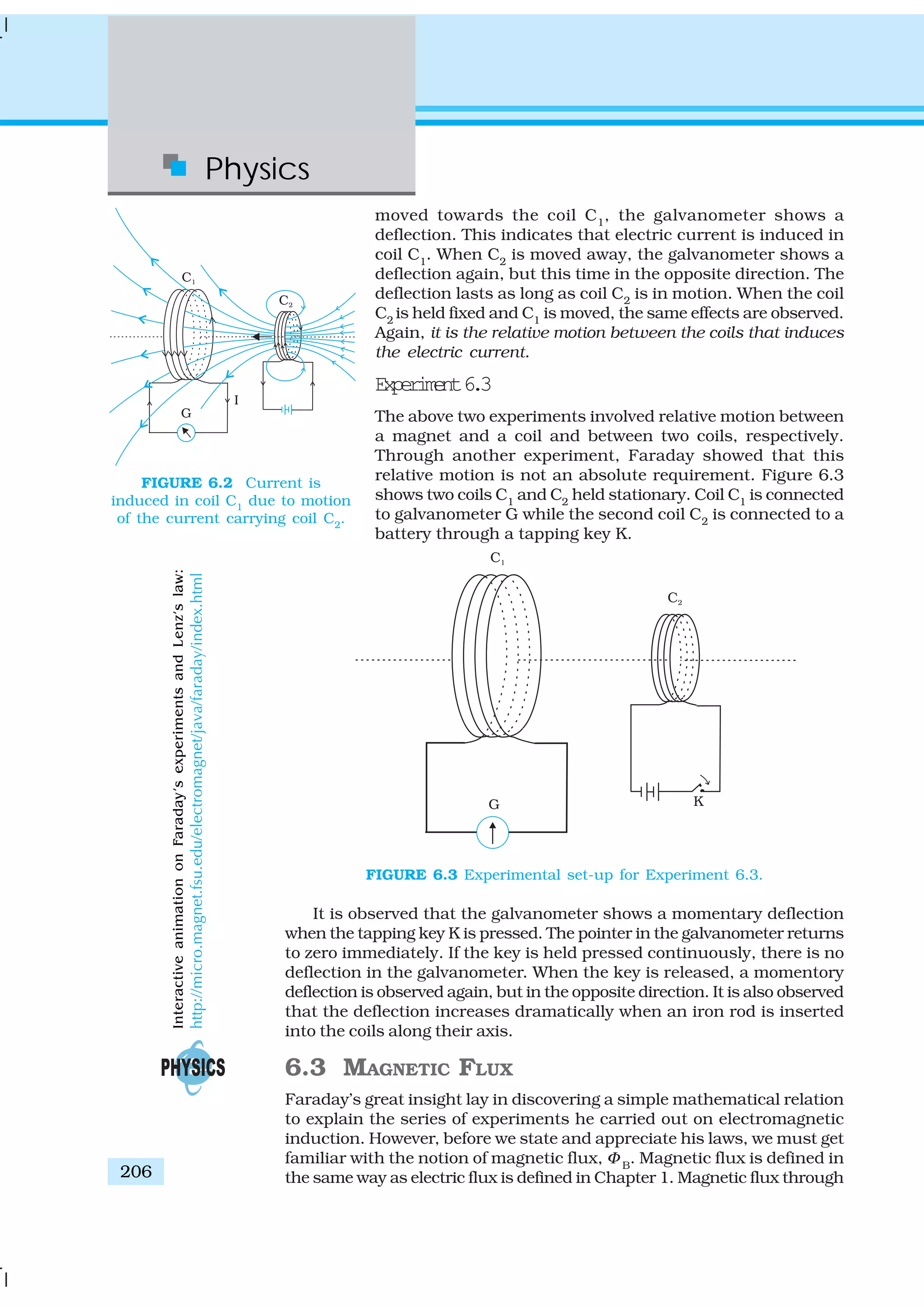
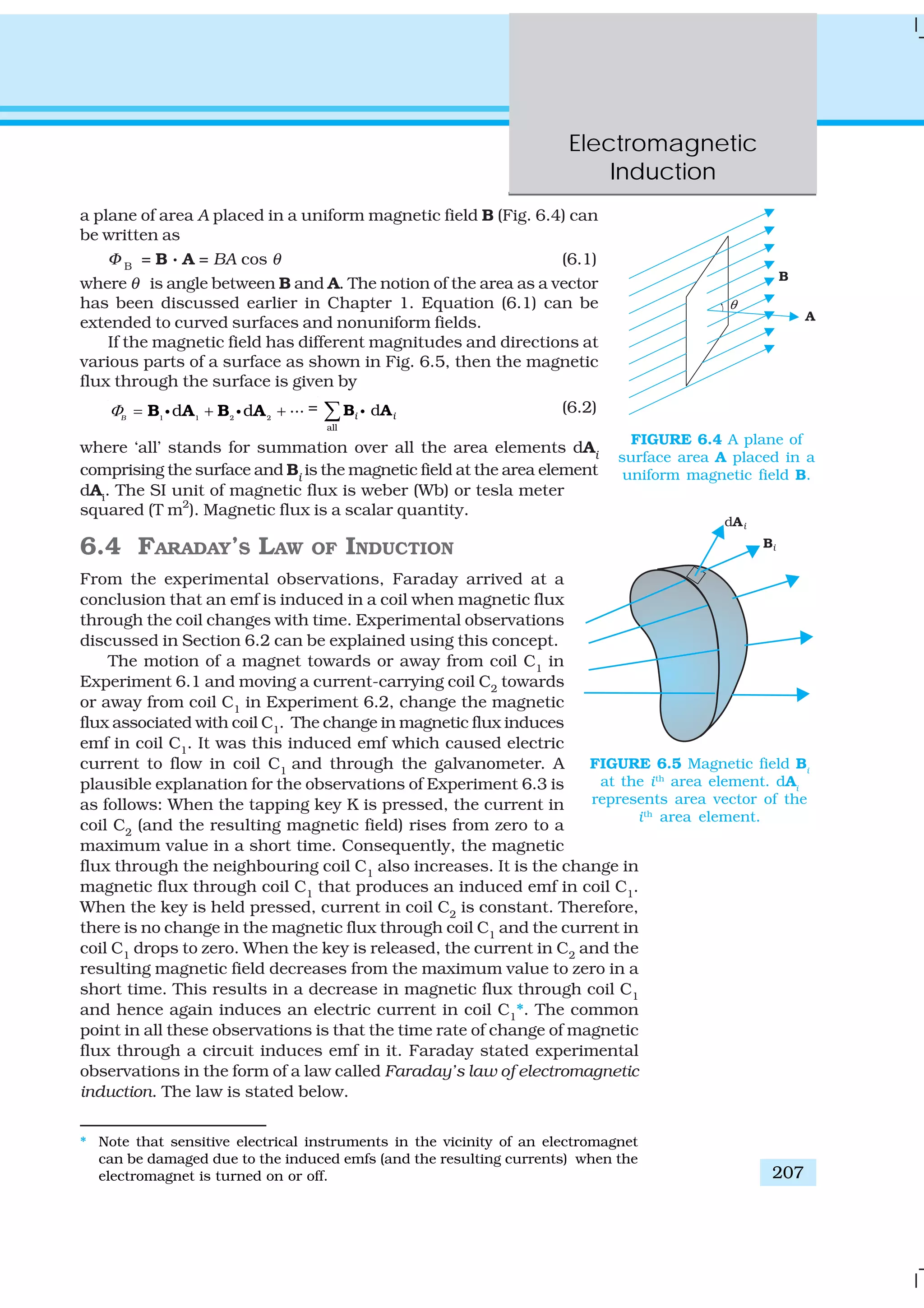
212. Physics
208
EXAMPLE6.1
The magnitude of the induced emf in a circuit is equal
to the time rate of change of magnetic flux through the
circuit.
Mathematically, the induced emf is given by
d
–
d
B
t
Φ
ε = (6.3)
The negative sign indicates the direction of ε and hence
the direction of current in a closed loop. This will be
discussed in detail in the next section.
In the case of a closely wound coil of N turns, change
of flux associated with each turn, is the same. Therefore,
the expression for the total induced emf is given by
d
–
d
B
N
t
Φ
ε = (6.4)
The induced emf can be increased by increasing the
number of turns N of a closed coil.
From Eqs. (6.1) and (6.2), we see that the flux can be
varied by changing any one or more of the terms B, A and
θ. In Experiments 6.1 and 6.2 in Section 6.2, the flux is
changed by varying B. The flux can also be altered by
changing the shape of a coil (that is, by shrinking it or
stretching it) in a magnetic field, or rotating a coil in a
magnetic field such that the angle θ between B and A
changes. In these cases too, an emf is induced in the
respective coils.
Example 6.1 Consider Experiment 6.2. (a) What would you do to obtain
a large deflection of the galvanometer? (b) How would you demonstrate
the presence of an induced current in the absence of a galvanometer?
Solution
(a) To obtain a large deflection, one or more of the following steps can
be taken: (i) Use a rod made of soft iron inside the coil C2
, (ii) Connect
the coil to a powerful battery, and (iii) Move the arrangement rapidly
towards the test coil C1
.
(b) Replace the galvanometer by a small bulb, the kind one finds in a
small torch light. The relative motion between the two coils will cause
the bulb to glow and thus demonstrate the presence of an induced
current.
In experimental physics one must learn to innovate. Michael Faraday
who is ranked as one of the best experimentalists ever, was legendary
for his innovative skills.
Example 6.2 A square loop of side 10 cm and resistance 0.5 Ω is
placed vertically in the east-west plane. A uniform magnetic field of
0.10 T is set up across the plane in the north-east direction. The
magnetic field is decreased to zero in 0.70 s at a steady rate. Determine
the magnitudes of induced emf and current during this time-interval.
Michael Faraday [1791–
1867] Faraday made
numerous contributions to
science, viz., the discovery
of electromagnetic
induction, the laws of
electrolysis, benzene, and
the fact that the plane of
polarisation is rotated in an
electric field. He is also
credited with the invention
of the electric motor, the
electric generator and the
transformer. He is widely
regarded as the greatest
experimental scientist of
the nineteenth century.
MICHAELFARADAY(1791–1867)
EXAMPLE6.2

213. Electromagnetic
Induction
209
EXAMPLE6.2
Solution The angle θ made by the area vector of the coil with the
magnetic field is 45°
. From Eq. (6.1), the initial magnetic flux is
Φ = BA cos θ
–2
0.1 10
Wb
2
×
=
Final flux, Φmin
= 0
The change in flux is brought about in 0.70 s. From Eq. (6.3), the
magnitude of the induced emf is given by
( )– 0B
t t
ΦΦ
ε
Δ
= =
Δ Δ
–3
10
= 1.0 mV
2 0.7
=
×
And the magnitude of the current is
–3
10 V
2 mA
0.5
I
R
ε
= = =
Ω
Note that the earth’s magnetic field also produces a flux through the
loop. But it is a steady field (which does not change within the time
span of the experiment) and hence does not induce any emf.
Example 6.3
A circular coil of radius 10 cm, 500 turns and resistance 2 Ω is placed
with its plane perpendicular to the horizontal component of the earth’s
magnetic field. It is rotated about its vertical diameter through 180°
in 0.25 s. Estimate the magnitudes of the emf and current induced in
the coil. Horizontal component of the earth’s magnetic field at the
place is 3.0 × 10–5
T.
Solution
Initial flux through the coil,
ΦB (initial)
= BA cos θ
= 3.0 × 10–5
× (π ×10–2
) × cos 0º
= 3π × 10–7
Wb
Final flux after the rotation,
ΦB (final)
= 3.0 × 10–5
× (π ×10–2
) × cos 180°
= –3π × 10–7
Wb
Therefore, estimated value of the induced emf is,
N
t
Φ
ε
Δ
=
Δ
= 500 × (6π × 10–7
)/0.25
= 3.8 × 10–3
V
I = ε/R = 1.9 × 10–3
A
Note that the magnitudes of ε and I are the estimated values. Their
instantaneous values are different and depend upon the speed of
rotation at the particular instant.
EXAMPLE6.3

214. Physics
210
6.5 LENZ’S LAW AND CONSERVATION OF ENERGY
In 1834, German physicist Heinrich Friedrich Lenz (1804-1865) deduced
a rule, known as Lenz’s law which gives the polarity of the induced emf
in a clear and concise fashion. The statement of the law is:
The polarity of induced emf is such that it tends to produce a current
which opposes the change in magnetic flux that produced it.
The negative sign shown in Eq. (6.3) represents this effect. We can
understand Lenz’s law by examining Experiment 6.1 in Section 6.2.1. In
Fig. 6.1, we see that the North-pole of a bar magnet is being pushed
towards the closed coil. As the North-pole of the bar magnet moves towards
the coil, the magnetic flux through the coil increases. Hence current is
induced in the coil in such a direction that it opposes the increase in flux.
This is possible only if the current in the coil is in a counter-clockwise
direction with respect to an observer situated on the side of the magnet.
Note that magnetic moment associated with this current has North polarity
towards the North-pole of the approaching magnet. Similarly, if the North-
pole of the magnet is being withdrawn from the coil, the magnetic flux
through the coil will decrease. To counter this decrease in magnetic flux,
the induced current in the coil flows in clockwise direction and its South-
pole faces the receding North-pole of the bar magnet. This would result in
an attractive force which opposes the motion of the magnet and the
corresponding decrease in flux.
What will happen if an open circuit is used in place of the closed loop
in the above example? In this case too, an emf is induced across the open
ends of the circuit. The direction of the induced emf can be found
using Lenz’s law. Consider Figs. 6.6 (a) and (b). They provide an easier
way to understand the direction of induced currents. Note that the
direction shown by and indicate the directions of the induced
currents.
A little reflection on this matter should convince us on the
correctness of Lenz’s law. Suppose that the induced current was in
the direction opposite to the one depicted in Fig. 6.6(a). In that case,
the South-pole due to the induced current will face the approaching
North-pole of the magnet. The bar magnet will then be attracted
towards the coil at an ever increasing acceleration. A gentle push on
the magnet will initiate the process and its velocity and kinetic energy
will continuously increase without expending any energy. If this can
happen, one could construct a perpetual-motion machine by a
suitable arrangement. This violates the law of conservation of energy
and hence can not happen.
Now consider the correct case shown in Fig. 6.6(a). In this situation,
the bar magnet experiences a repulsive force due to the induced
current. Therefore, a person has to do work in moving the magnet.
Where does the energy spent by the person go? This energy is
dissipated by Joule heating produced by the induced current.
FIGURE 6.6
Illustration of
Lenz’s law.

215. Electromagnetic
Induction
211
EXAMPLE6.4
Example 6.4
Figure 6.7 shows planar loops of different shapes moving out of or
into a region of a magnetic field which is directed normal to the plane
of the loop away from the reader. Determine the direction of induced
current in each loop using Lenz’s law.
FIGURE 6.7
Solution
(i) The magnetic flux through the rectangular loop abcd increases,
due to the motion of the loop into the region of magnetic field, The
induced current must flow along the path bcdab so that it opposes
the increasing flux.
(ii) Due to the outward motion, magnetic flux through the triangular
loop abc decreases due to which the induced current flows along
bacb, so as to oppose the change in flux.
(iii) As the magnetic flux decreases due to motion of the irregular
shaped loop abcd out of the region of magnetic field, the induced
current flows along cdabc, so as to oppose change in flux.
Note that there are no induced current as long as the loops are
completely inside or outside the region of the magnetic field.
Example 6.5
(a) A closed loop is held stationary in the magnetic field between the
north and south poles of two permanent magnets held fixed. Can
we hope to generate current in the loop by using very strong
magnets?
(b) A closed loop moves normal to the constant electric field between
the plates of a large capacitor. Is a current induced in the loop
(i) when it is wholly inside the region between the capacitor plates
(ii) when it is partially outside the plates of the capacitor? The
electric field is normal to the plane of the loop.
(c) A rectangular loop and a circular loop are moving out of a uniform
magnetic field region (Fig. 6.8) to a field-free region with a constant
velocity v. In which loop do you expect the induced emf to be
constant during the passage out of the field region? The field is
normal to the loops.
EXAMPLE6.5

216. Physics
212
EXAMPLE6.5
FIGURE 6.8
(d) Predict the polarity of the capacitor in the situation described by
Fig. 6.9.
FIGURE 6.9
Solution
(a) No. However strong the magnet may be, current can be induced
only by changing the magnetic flux through the loop.
(b) No current is induced in either case. Current can not be induced
by changing the electric flux.
(c) The induced emf is expected to be constant only in the case of the
rectangular loop. In the case of circular loop, the rate of change of
area of the loop during its passage out of the field region is not
constant, hence induced emf will vary accordingly.
(d) The polarity of plate ‘A’ will be positive with respect to plate ‘B’ in
the capacitor.
6.6 MOTIONAL ELECTROMOTIVE FORCE
Let us consider a straight conductor moving in a uniform and time-
independent magnetic field. Figure 6.10 shows a rectangular conductor
PQRS in which the conductor PQ is free to move. The rod PQ is moved
towards the left with a constant velocity v as
shown in the figure. Assume that there is no
loss of energy due to friction. PQRS forms a
closed circuit enclosing an area that changes
as PQ moves. It is placed in a uniform magnetic
field B which is perpendicular to the plane of
this system. If the length RQ = x and RS = l, the
magnetic flux ΦB
enclosed by the loop PQRS
will be
ΦB
= Blx
Since x is changing with time, the rate of change
of flux ΦB
will induce an emf given by:
( )
– d d
–
d d
B
Blx
t t
Φ
ε = =
=
d
–
d
x
Bl Blv
t
= (6.5)
FIGURE 6.10 The arm PQ is moved to the left
side, thus decreasing the area of the
rectangular loop. This movement
induces a current I as shown.

217. Electromagnetic
Induction
213
where we have used dx/dt = –v which is the speed of the conductor PQ.
The induced emf Blv is called motional emf. Thus, we are able to produce
induced emf by moving a conductor instead of varying the magnetic field,
that is, by changing the magnetic flux enclosed by the circuit.
It is also possible to explain the motional emf expression in Eq. (6.5)
by invoking the Lorentz force acting on the free charge carriers of conductor
PQ. Consider any arbitrary charge q in the conductor PQ. When the rod
moves with speed v, the charge will also be moving with speed v in the
magnetic field B. The Lorentz force on this charge is qvB in magnitude,
and its direction is towards Q. All charges experience the same force, in
magnitude and direction, irrespective of their position in the rod PQ.
The work done in moving the charge from P to Q is,
W = qvBl
Since emf is the work done per unit charge,
W
q
ε =
= Blv
This equation gives emf induced across the rod PQ and is identical
to Eq. (6.5). We stress that our presentation is not wholly rigorous. But
it does help us to understand the basis of Faraday’s law when
the conductor is moving in a uniform and time-independent
magnetic field.
On the other hand, it is not obvious how an emf is induced when a
conductor is stationary and the magnetic field is changing – a fact which
Faraday verified by numerous experiments. In the case of a stationary
conductor, the force on its charges is given by
F = q (E + v × B) = qE (6.6)
since v = 0. Thus, any force on the charge must arise from the electric
field term E alone. Therefore, to explain the existence of induced emf or
induced current, we must assume that a time-varying magnetic field
generates an electric field. However, we hasten to add that electric fields
produced by static electric charges have properties different from those
produced by time-varying magnetic fields. In Chapter 4, we learnt that
charges in motion (current) can exert force/torque on a stationary magnet.
Conversely, a bar magnet in motion (or more generally, a changing
magnetic field) can exert a force on the stationary charge. This is the
fundamental significance of the Faraday’s discovery. Electricity and
magnetism are related.
Example 6.6 A metallic rod of 1 m length is rotated with a frequency
of 50 rev/s, with one end hinged at the centre and the other end at the
circumference of a circular metallic ring of radius 1 m, about an axis
passing through the centre and perpendicular to the plane of the ring
(Fig. 6.11). A constant and uniform magnetic field of 1 T parallel to the
axis is present everywhere. What is the emf between the centre and
the metallic ring?
EXAMPLE6.6
Interactiveanimationonmotionalemf:
http://www.ngsir,netfirms.com/englishhtm/Induction.htm

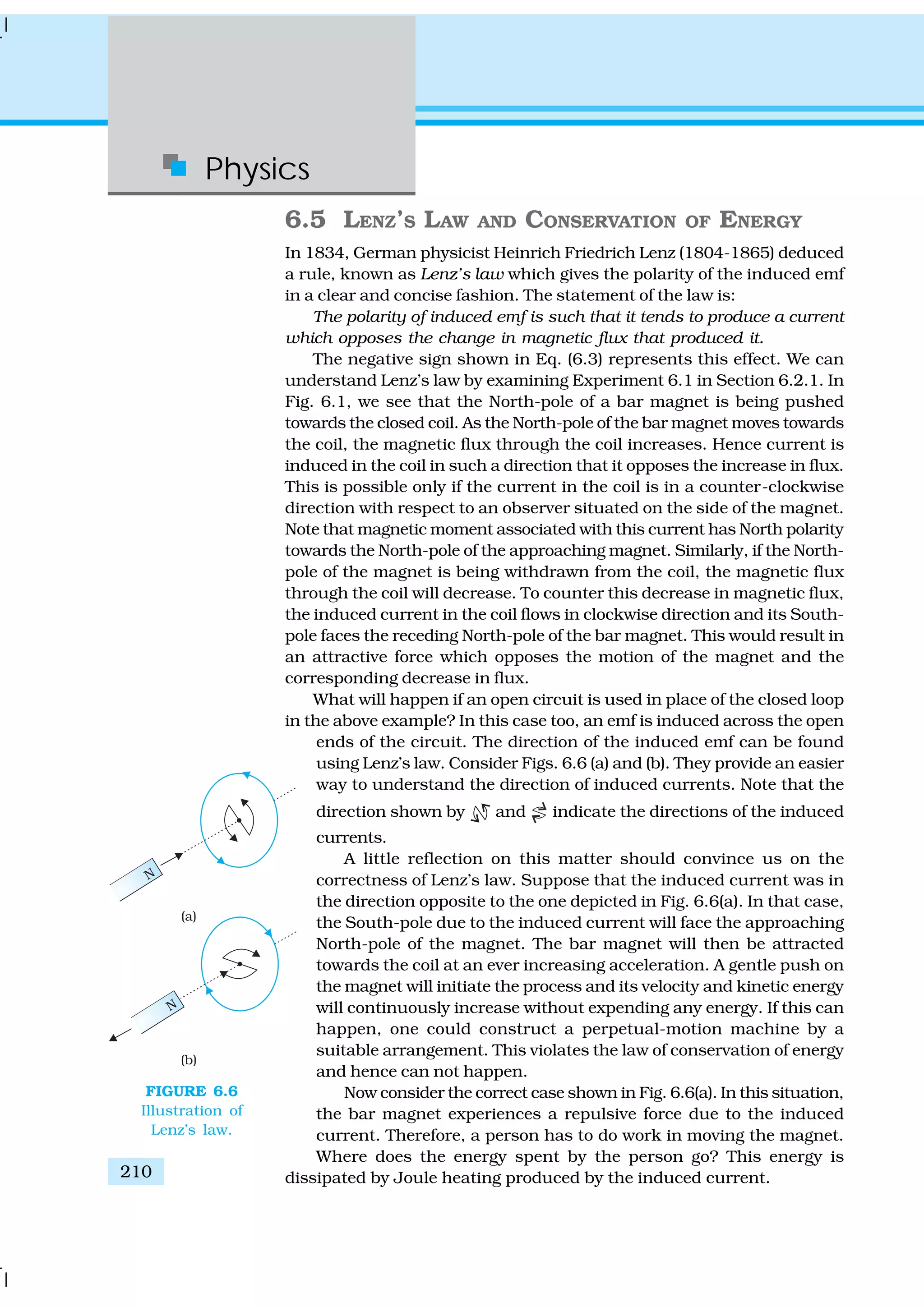
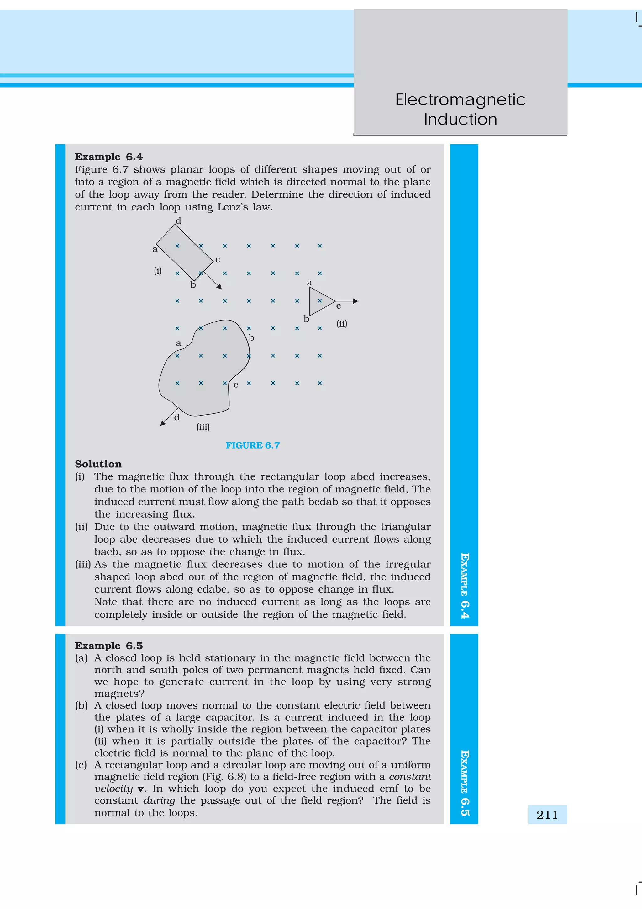
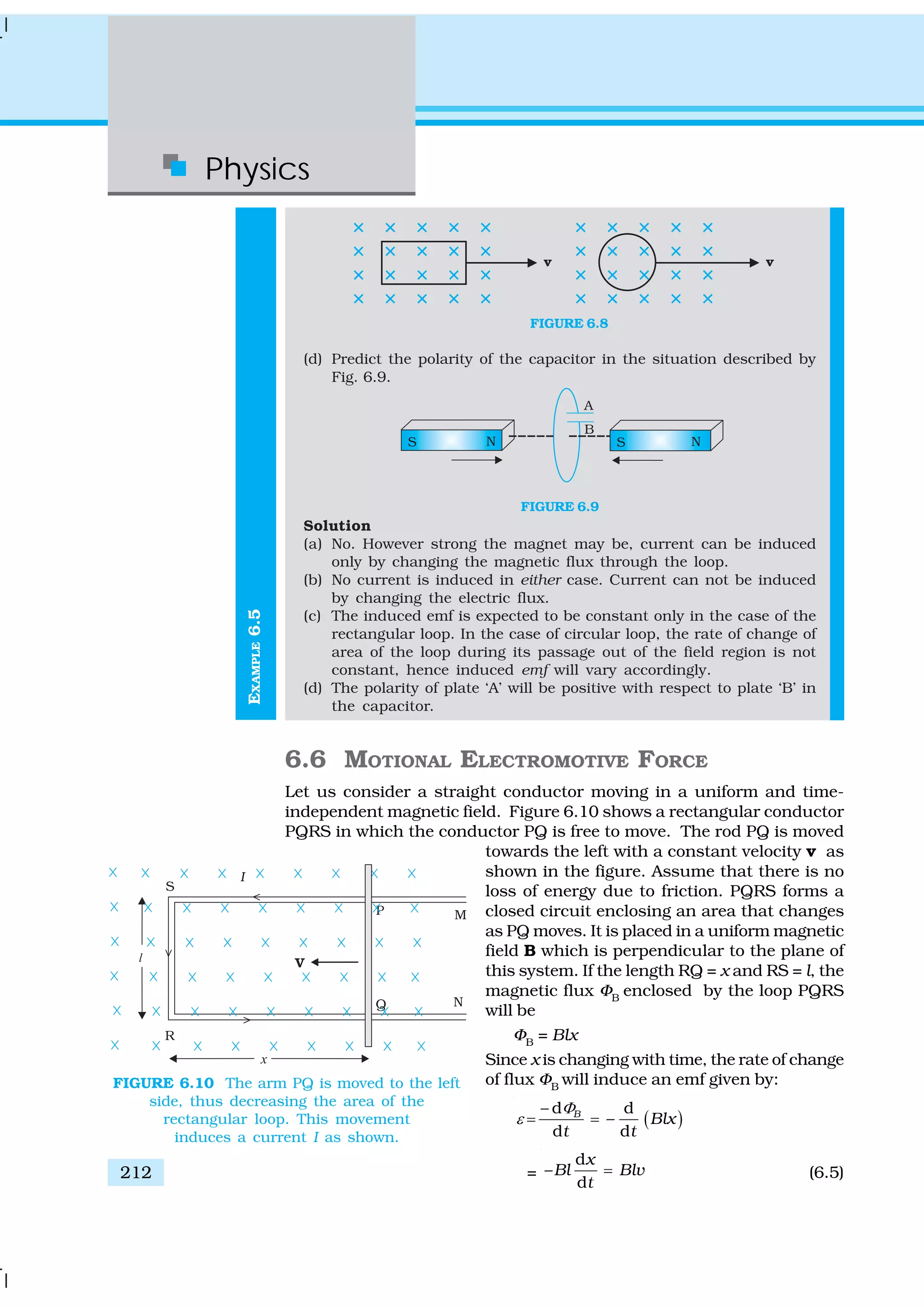
218. Physics
214
EXAMPLE6.6
FIGURE 6.11
Solution
Method I
As the rod is rotated, free electrons in the rod move towards the outer
end due to Lorentz force and get distributed over the ring. Thus, the
resulting separation of charges produces an emf across the ends of
the rod. At a certain value of emf, there is no more flow of electrons
and a steady state is reached. Using Eq. (6.5), the magnitude of the
emf generated across a length dr of the rod as it moves at right angles
to the magnetic field is given by
d dBv rε = . Hence,
0
d d
R
Bv rε ε= =∫ ∫
2
0
d
2
R
B R
B r r
ω
ω= =∫
Note that we have used v = ω r. This gives
ε
21
1.0 2 50 (1 )
2
= × × π × ×
= 157 V
Method II
To calculate the emf, we can imagine a closed loop OPQ in which
point O and P are connected with a resistor R and OQ is the rotating
rod. The potential difference across the resistor is then equal to the
induced emf and equals B × (rate of change of area of loop). If θ is the
angle between the rod and the radius of the circle at P at time t, the
area of the sector OPQ is given by
2 21
2 2
R R
θ
θπ × =
π
where R is the radius of the circle. Hence, the induced emf is
ε =
2d 1
d 2
B R
t
θ
⎡ ⎤
× ⎢ ⎥⎣ ⎦
=
2
21 d
2 d 2
B R
BR
t
θ ω
=
[Note:
d
2
dt
θ
ω ν= = π ]
This expression is identical to the expression obtained by Method I
and we get the same value of ε.

219. Electromagnetic
Induction
215
EXAMPLE6.7
Example 6.7
A wheel with 10 metallic spokes each 0.5 m long is rotated with a
speed of 120 rev/min in a plane normal to the horizontal component
of earth’s magnetic field HE
at a place. If HE
= 0.4 G at the place, what
is the induced emf between the axle and the rim of the wheel? Note
that 1 G = 10–4
T.
Solution
Induced emf = (1/2) ω B R2
= (1/2) × 4π × 0.4 × 10–4
× (0.5)2
= 6.28 × 10–5
V
The number of spokes is immaterial because the emf’s across the
spokes are in parallel.
6.7 ENERGY CONSIDERATION: A QUANTITATIVE STUDY
InSection6.5,wediscussedqualitativelythatLenz’slawisconsistentwith
the law of conservation of energy. Now we shall explore this aspect further
with a concrete example.
Let r be the resistance of movable arm PQ of the rectangular conductor
shown in Fig. 6.10. We assume that the remaining arms QR, RS and SP
have negligible resistances compared to r. Thus, the overall resistance of
the rectangular loop is r and this does not change as PQ is moved. The
current I in the loop is,
I
r
ε
=
=
B l v
r
(6.7)
On account of the presence of the magnetic field, there will be a force
on the arm PQ. This force I (l ×× B), is directed outwards in the direction
opposite to the velocity of the rod. The magnitude of this force is,
F = I l B =
2 2
B l v
r
where we have used Eq. (6.7). Note that this force arises due to drift velocity
of charges (responsible for current) along the rod and the consequent
Lorentz force acting on them.
Alternatively, the arm PQ is being pushed with a constant speed v,
the power required to do this is,
P F v=
=
2 2 2
B l v
r
(6.8)
The agent that does this work is mechanical. Where does this
mechanical energy go? The answer is: it is dissipated as Joule heat, and
is given by
2
JP I r=
2
Blv
r
r
⎛ ⎞
= ⎜ ⎟⎝ ⎠
2 2 2
B l v
r
=
which is identical to Eq. (6.8).

220. Physics
216
EXAMPLE6.8
Thus, mechanical energy which was needed to move the arm PQ is
converted into electrical energy (the induced emf) and then to thermal energy.
There is an interesting relationship between the charge flow through
the circuit and the change in the magnetic flux. From Faraday’s law, we
have learnt that the magnitude of the induced emf is,
B
t
Φ
ε
Δ
=
Δ
However,
Q
Ir r
t
ε
Δ
= =
Δ
Thus,
B
Q
r
ΦΔ
Δ =
Example 6.8 Refer to Fig. 6.12(a). The arm PQ of the rectangular
conductor is moved from x = 0, outwards. The uniform magnetic field is
perpendicular to the plane and extends from x = 0 to x = b and is zero
for x > b. Only the arm PQ possesses substantial resistance r. Consider
the situation when the arm PQ is pulled outwards from x = 0 to x = 2b,
and is then moved back to x = 0 with constant speed v. Obtain expressions
for the flux, the induced emf, the force necessary to pull the arm and the
power dissipated as Joule heat. Sketch the variation of these quantities
with distance.
(a)
FIGURE 6.12
Solution Let us first consider the forward motion from x = 0 to x = 2b
The flux ΦB
linked with the circuit SPQR is
B 0Bl x x bΦ = ≤ <
2Bl b b x b= ≤ <
The induced emf is,
Bd
dt
Φ
ε = −
0Blv x b= − ≤ <
0 2b x b= ≤ <

221. Electromagnetic
Induction
217
EXAMPLE6.8
When the induced emf is non-zero, the current I is (in magnitude)
Bl v
I
r
=
(b)
FIGURE 6.12
The force required to keep the arm PQ in constant motion is I lB. Its
direction is to the left. In magnitude
2 2
0
0 2
B l v
F x b
r
b x b
= ≤ <
= ≤ <
The Joule heating loss is
2
JP I r=
2 2 2
0
0 2
B l v
x b
r
b x b
= ≤ <
= ≤ <
One obtains similar expressions for the inward motion from x = 2b to
x = 0. One can appreciate the whole process by examining the sketch
of various quantities displayed in Fig. 6.12(b).

222. Physics
218
6.8 EDDY CURRENTS
So far we have studied the electric currents induced in well defined paths
in conductors like circular loops. Even when bulk pieces of conductors
are subjected to changing magnetic flux, induced currents
are produced in them. However, their flow patterns resemble
swirling eddies in water. This effect was discovered by physicist
Foucault (1819-1868) and these currents are called eddy
currents.
Consider the apparatus shown in Fig. 6.13. A copper plate
is allowed to swing like a simple pendulum between the pole
pieces of a strong magnet. It is found that the motion is damped
and in a little while the plate comes to a halt in the magnetic
field. We can explain this phenomenon on the basis of
electromagnetic induction. Magnetic flux associated with the
plate keeps on changing as the plate moves in and out of the
region between magnetic poles. The flux change induces eddy
currents in the plate. Directions of eddy currents are opposite
when the plate swings into the region between the poles and
when it swings out of the region.
If rectangular slots are made in the copper plate as shown
in Fig. 6.14, area available to the flow of eddy currents is less.
Thus, the pendulum plate with holes or slots reduces
electromagnetic damping and the plate swings more freely.
Note that magnetic moments of the induced currents (which
oppose the motion) depend upon the area enclosed by the
currents (recall equation m = IA in Chapter 4).
This fact is helpful in reducing eddy currents in the metallic
cores of transformers, electric motors and other such devices in
which a coil is to be wound over metallic core. Eddy currents are
undesirable since they heat up the core and dissipate electrical
energy in the form of heat. Eddy currents are minimised by using
laminations of metal to make a metal core. The laminations are
separated by an insulating material like lacquer. The plane of the
laminations must be arranged parallel to the magnetic field, so
that they cut across the eddy current paths. This arrangement
reduces the strength of the eddy currents. Since the dissipation
of electrical energy into heat depends on the square of the strength
of electric current, heat loss is substantially reduced.
Eddy currents are used to advantage in certain applications like:
(i) Magnetic braking in trains: Strong electromagnets are situated
above the rails in some electrically powered trains. When the
electromagnets are activated, the eddy currents induced in the
rails oppose the motion of the train. As there are no mechanical
linkages, the braking effect is smooth.
(ii) Electromagnetic damping: Certain galvanometers have a fixed
core made of nonmagnetic metallic material. When the coil
oscillates, the eddy currents generated in the core oppose the
motion and bring the coil to rest quickly.
FIGURE 6.13 Eddy currents are
generated in the copper plate,
while entering
and leaving the region of
magnetic field.
FIGURE 6.14 Cutting slots
in the copper plate reduces
the effect of eddy currents.

223. Electromagnetic
Induction
219
(iii) Induction furnace: Induction furnace can be used to produce high
temperatures and can be utilised to prepare alloys, by melting the
constituent metals. A high frequency alternating current is passed
through a coil which surrounds the metals to be melted. The eddy
currents generated in the metals produce high temperatures sufficient
to melt it.
(iv) Electric power meters: The shiny metal disc in the electric power meter
(analogue type) rotates due to the eddy currents. Electric currents
are induced in the disc by magnetic fields produced by sinusoidally
varying currents in a coil.
You can observe the rotating shiny disc in the power meter of your
house.
ELECTROMAGNETIC DAMPING
Take two hollow thin cylindrical pipes of equal internal diameters made of aluminium and
PVC, respectively. Fix them vertically with clamps on retort stands. Take a small cylinderical
magnet having diameter slightly smaller than the inner diameter of the pipes and drop it
through each pipe in such a way that the magnet does not touch the sides of the pipes
during its fall. You will observe that the magnet dropped through the PVC pipe takes the
same time to come out of the pipe as it would take when dropped through the same height
without the pipe. Note the time it takes to come out of the pipe in each case. You will see that
the magnet takes much longer time in the case of aluminium pipe. Why is it so? It is due to
the eddy currents that are generated in the aluminium pipe which oppose the change in
magnetic flux, i.e., the motion of the magnet. The retarding force due to the eddy currents
inhibits the motion of the magnet. Such phenomena are referred to as electromagnetic damping.
Note that eddy currents are not generated in PVC pipe as its material is an insulator whereas
aluminium is a conductor.
6.9 INDUCTANCE
An electric current can be induced in a coil by flux change produced by
another coil in its vicinity or flux change produced by the same coil. These
two situations are described separately in the next two sub-sections.
However, in both the cases, the flux through a coil is proportional to the
current. That is, ΦB
α I.
Further, if the geometry of the coil does not vary with time then,
d d
d d
B I
t t
Φ
∝
For a closely wound coil of N turns, the same magnetic flux is linked
with all the turns. When the flux ΦB
through the coil changes, each turn
contributes to the induced emf. Therefore, a term called flux linkage is
used which is equal to NΦB
for a closely wound coil and in such a case
NΦB ∝ I
The constant of proportionality, in this relation, is called inductance.
We shall see that inductance depends only on the geometry of the coil

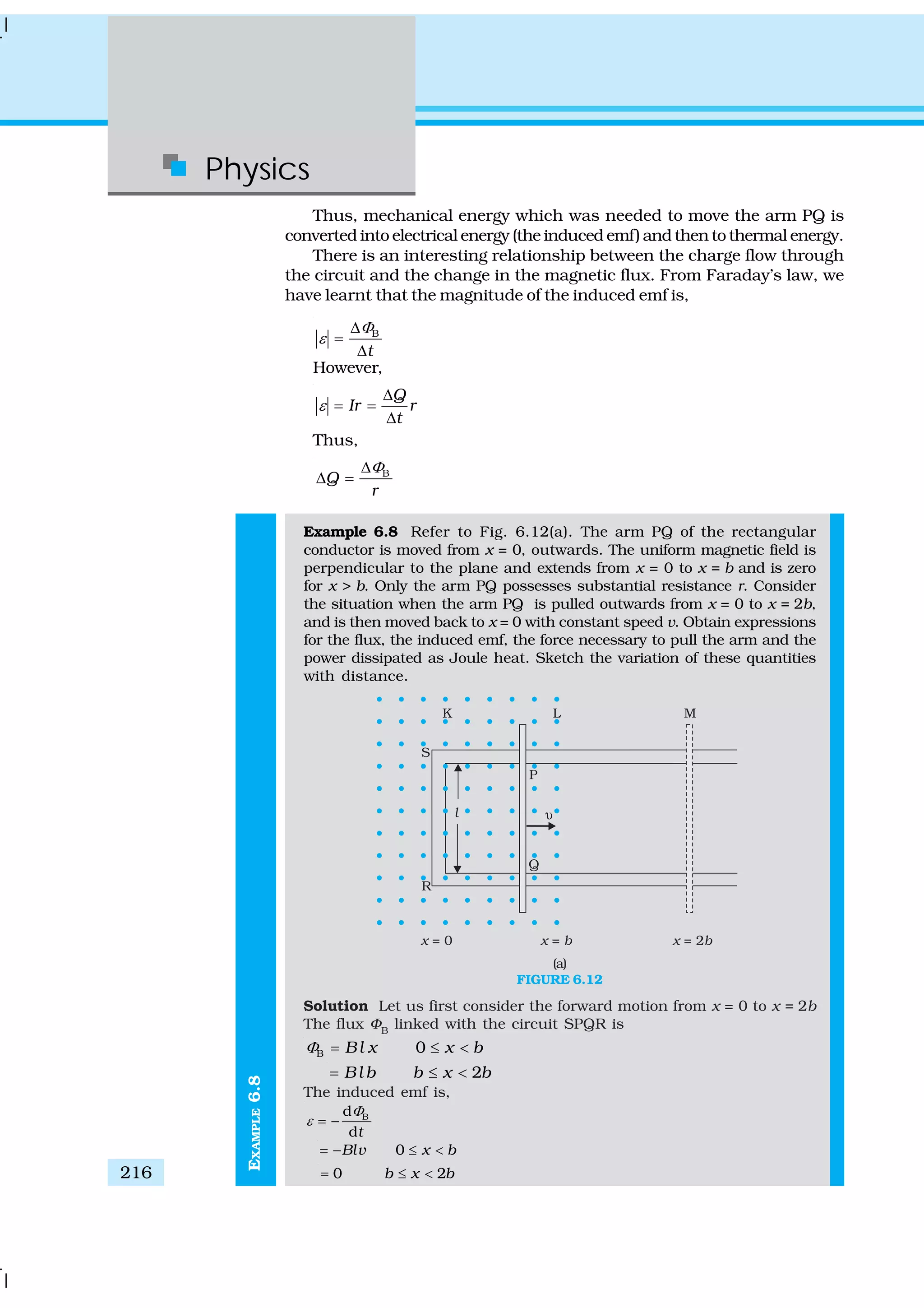
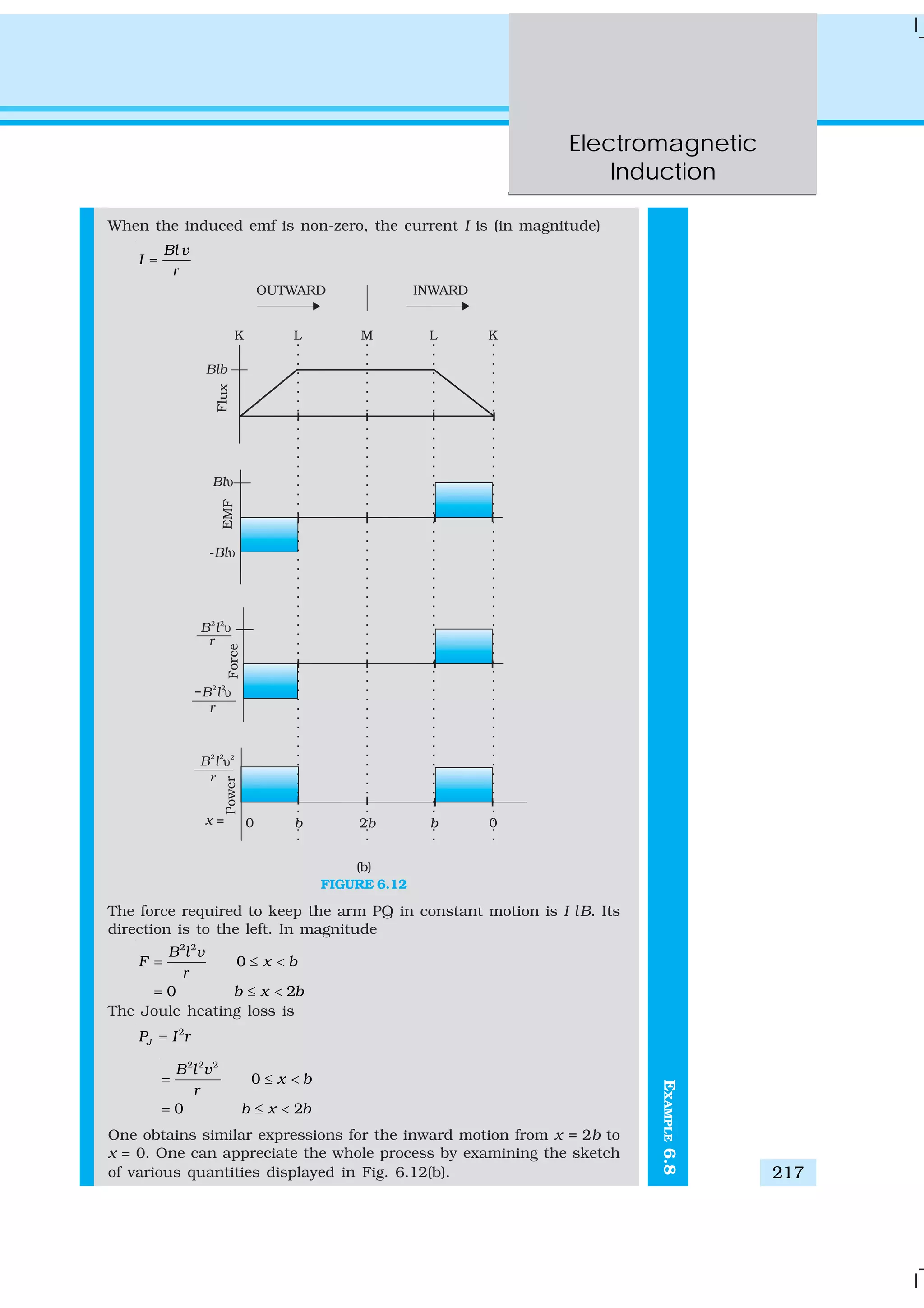
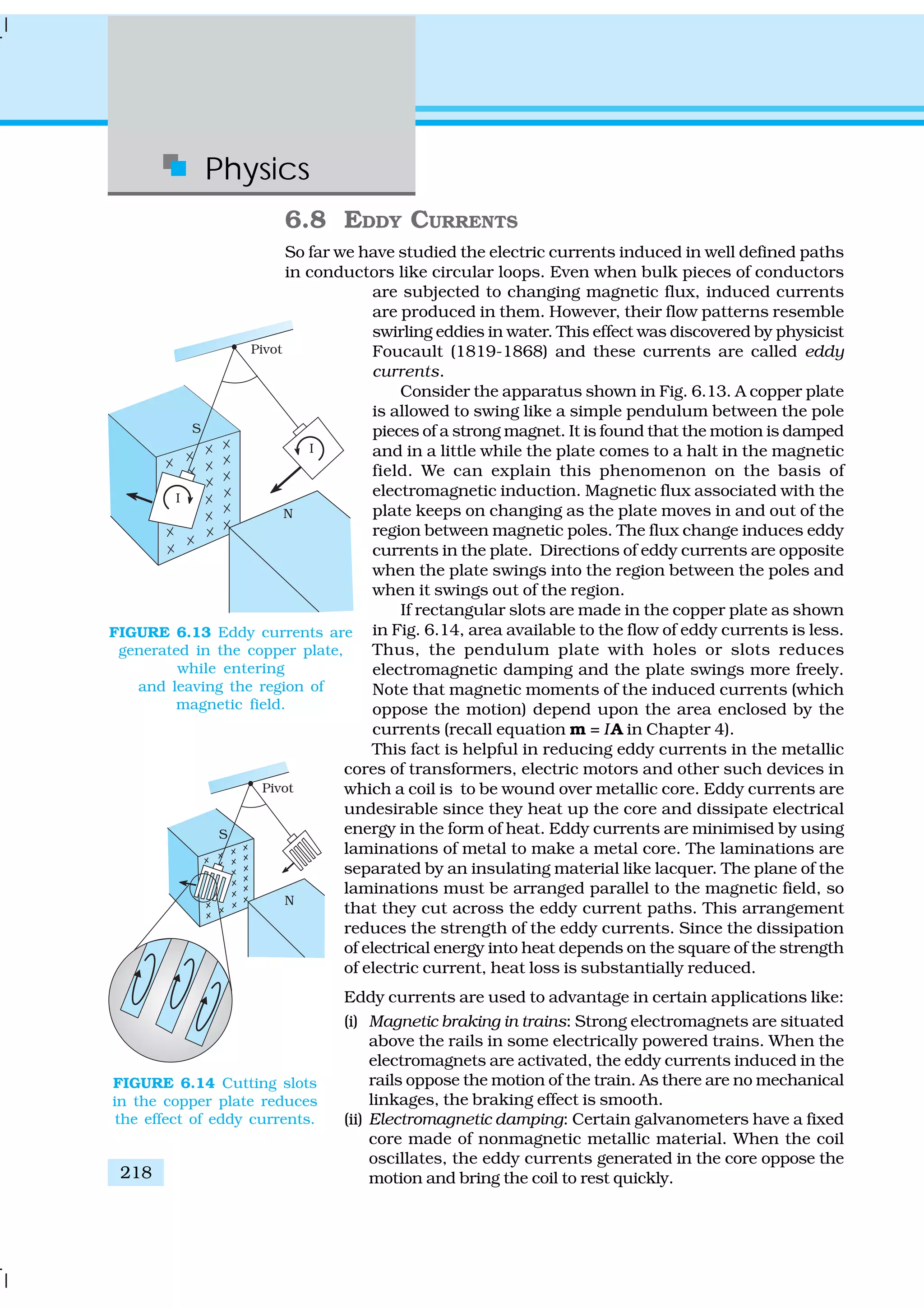
224. Physics
220
and intrinsic material properties. This aspect is akin to capacitance which
for a parallel plate capacitor depends on the plate area and plate separation
(geometry) and the dielectric constant K of the intervening medium
(intrinsic material property).
Inductance is a scalar quantity. It has the dimensions of [M L2
T–2
A–2
]
given by the dimensions of flux divided by the dimensions of current. The
SI unit of inductance is henry and is denoted by H. It is named in honour
of Joseph Henry who discovered electromagnetic induction in USA,
independently of Faraday in England.
6.9.1 Mutual inductance
Consider Fig. 6.15 which shows two long co-axial solenoids each of length
l. We denote the radius of the inner solenoid S1
by r1
and the number of
turns per unit length by n1
. The corresponding quantities for the outer
solenoid S2
are r2
and n2
, respectively. Let N1
and N2
be the total number
of turns of coils S1
and S2
, respectively.
When a current I2
is set up through S2
, it in turn sets up a magnetic
flux through S1
. Let us denote it by Φ1
. The corresponding flux linkage
with solenoid S1
is
N1 1 12 2M IΦ = (6.9)
M12
is called the mutual inductance of solenoid S1
with respect to
solenoid S2
. It is also referred to as the coefficient of mutual induction.
For these simple co-axial solenoids it is possible to calculate M12
. The
magnetic field due to the current I2
in S2
is μ0
n2
I2
. The resulting flux linkage
with coil S1
is,
( ) ( ) ( )2
1 1 1 1 0 2 2N n l r n IΦ μ= π
2
0 1 2 1 2n n r l Iμ= π (6.10)
where n1
l is the total number of turns in solenoid S1
. Thus, from Eq. (6.9)
and Eq. (6.10),
M12
= μ0
n1
n2
πr 2
1
l (6.11)
Note that we neglected the edge effects and considered
the magnetic field μ0
n2
I2
to be uniform throughout the
length and width of the solenoid S2
. This is a good
approximation keeping in mind that the solenoid is long,
implying l >> r2
.
We now consider the reverse case. A current I1
is
passed through the solenoid S1
and the flux linkage with
coil S2
is,
N2
Φ2
= M21
I1
(6.12)
M21
is called the mutual inductance of solenoid S2
with
respect to solenoid S1
.
The flux due to the current I1
in S1
can be assumed to
be confined solely inside S1
since the solenoids are very
long. Thus, flux linkage with solenoid S2
is
( ) ( ) ( )2
2 2 2 1 0 1 1N n l r n IΦ μ= π
FIGURE 6.15 Two long co-axial
solenoids of same
length l.

225. Electromagnetic
Induction
221
EXAMPLE6.9
where n2
l is the total number of turns of S2
. From Eq. (6.12),
M21
= μ0
n1
n2
πr2
1
l (6.13)
Using Eq. (6.11) and Eq. (6.12), we get
M12
= M21
= M (say) (6.14)
We have demonstrated this equality for long co-axial solenoids.
However, the relation is far more general. Note that if the inner solenoid
was much shorter than (and placed well inside) the outer solenoid, then
we could still have calculated the flux linkage N1
Φ1
because the inner
solenoid is effectively immersed in a uniform magnetic field due to the
outer solenoid. In this case, the calculation of M12
would be easy. However,
it would be extremely difficult to calculate the flux linkage with the outer
solenoid as the magnetic field due to the inner solenoid would vary across
the length as well as cross section of the outer solenoid. Therefore, the
calculation of M21
would also be extremely difficult in this case. The
equality M12
=M21
is very useful in such situations.
We explained the above example with air as the medium within the
solenoids. Instead, if a medium of relative permeability μr
had been present,
the mutual inductance would be
M =μr
μ0
n1
n2
π r2
1
l
It is also important to know that the mutual inductance of a pair of
coils, solenoids, etc., depends on their separation as well as their relative
orientation.
Example 6.9 Two concentric circular coils, one of small radius r1
and
the other of large radius r2
, such that r1
<< r2
, are placed co-axially
with centres coinciding. Obtain the mutual inductance of the
arrangement.
Solution Let a current I2
flow through the outer circular coil. The
field at the centre of the coil is B2
= μ0
I2
/ 2r2
. Since the other
co-axially placed coil has a very small radius, B2
may be considered
constant over its cross-sectional area. Hence,
Φ1
= πr 2
1
B2
2
0 1
2
22
r
I
r
μ π
=
= M12
I2
Thus,
2
0 1
12
22
r
M
r
μ π
=
From Eq. (6.14)
2
0 1
12 21
22
r
M M
r
μ π
= =
Note that we calculated M12
from an approximate value of Φ1
, assuming
the magnetic field B2
to be uniform over the area π r1
2
. However, we
can accept this value because r1
<< r2
.

226. Physics
222
Now, let us recollect Experiment 6.3 in Section 6.2. In that experiment,
emf is induced in coil C1
wherever there was any change in current through
coil C2
. Let Φ1
be the flux through coil C1
(say of N1
turns) when current in
coil C2
is I2
.
Then, from Eq. (6.9), we have
N1
Φ1
= MI2
For currents varrying with time,
( ) ( )1 1 2d d
d d
N MI
t t
Φ
=
Since induced emf in coil C1
is given by
( )1 1d
–
d
N
t
Φ
ε1 =
We get,
2d
–
d
I
M
t
ε1 =
It shows that varying current in a coil can induce emf in a neighbouring
coil. The magnitude of the induced emf depends upon the rate of change
of current and mutual inductance of the two coils.
6.9.2 Self-inductance
In the previous sub-section, we considered the flux in one solenoid due
to the current in the other. It is also possible that emf is induced in a
single isolated coil due to change of flux through the coil by means of
varying the current through the same coil. This phenomenon is called
self-induction. In this case, flux linkage through a coil of N turns is
proportional to the current through the coil and is expressed as
BN IΦ ∝
B LN IΦ = (6.15)
where constant of proportionality L is called self-inductance of the coil. It
is also called the coefficient of self-induction of the coil. When the current
is varied, the flux linked with the coil also changes and an emf is induced
in the coil. Using Eq. (6.15), the induced emf is given by
( )Bd
–
d
N
t
Φ
ε =
d
–
d
I
L
t
ε = (6.16)
Thus, the self-induced emf always opposes any change (increase or
decrease) of current in the coil.
It is possible to calculate the self-inductance for circuits with simple
geometries. Let us calculate the self-inductance of a long solenoid of cross-
sectional area A and length l, having n turns per unit length. The magnetic
field due to a current I flowing in the solenoid is B = μ0
n I (neglecting edge
effects, as before). The total flux linked with the solenoid is
( )( )( )0BN nl n I AΦ μ=

227. Electromagnetic
Induction
223
IAln2
0
μ=
where nl is the total number of turns. Thus, the self-inductance is,
L
I
ΒΝΦ
=
2
0n Alμ= (6.17)
If we fill the inside of the solenoid with a material of relative permeability
μr
(for example soft iron, which has a high value of relative permiability),
then,
2
0rL n Alμ μ= (6.18)
The self-inductance of the coil depends on its geometry and on the
permeability of the medium.
The self-induced emf is also called the back emf as it opposes any
change in the current in a circuit. Physically, the self-inductance plays
the role of inertia. It is the electromagnetic analogue of mass in mechanics.
So, work needs to be done against the back emf (ε) in establishing the
current. This work done is stored as magnetic potential energy. For the
current I at an instant in a circuit, the rate of work done is
d
d
W
I
t
ε=
If we ignore the resistive losses and consider only inductive effect,
then using Eq. (6.16),
d d
d d
W I
L I
t t
=
Total amount of work done in establishing the current I is
0
d d
I
W W L I I= =∫ ∫
Thus, the energy required to build up the current I is,
21
2
W LI= (6.19)
This expression reminds us of mv2
/2 for the (mechanical) kinetic energy
of a particle of mass m, and shows that L is analogus to m (i.e., L is electrical
inertia and opposes growth and decay of current in the circuit).
Consider the general case of currents flowing simultaneously in two
nearby coils. The flux linked with one coil will be the sum of two fluxes
which exist independently. Equation (6.9) would be modified into
N1 1 11 1 12 2M I M IΦ = +
where M11
represents inductance due to the same coil.
Therefore, using Faraday’s law,
1 2
1 11 12
d d
d d
I I
M M
t t
ε = − −

228. Physics
224
EXAMPLE6.10
M11
is the self-inductance and is written as L1
. Therefore,
1 2
1 1 12
d d
d d
I I
L M
t t
ε = − −
Example 6.10 (a) Obtain the expression for the magnetic energy stored
in a solenoid in terms of magnetic field B, area A and length l of the
solenoid. (b) How does this magnetic energy compare with the
electrostatic energy stored in a capacitor?
Solution
(a) From Eq. (6.19), the magnetic energy is
21
2
BU LI=
( )
2
1
since ,for a solenoid
2
0
0
B
L B nI
n
μ
μ
⎛ ⎞
= =⎜ ⎟⎝ ⎠
2
2
0
0
1
( )
2
B
n Al
n
μ
μ
⎛ ⎞
= ⎜ ⎟⎝ ⎠
[from Eq. (6.17)]
2
0
1
2
B Al
μ
=
(b) The magnetic energy per unit volume is,
B
B
U
u
V
= (where V is volume that contains flux)
BU
Al
=
2
02
B
μ
= (6.20)
We have already obtained the relation for the electrostatic energy
stored per unit volume in a parallel plate capacitor (refer to Chapter 2,
Eq. 2.77),
2
0
1
2
u EΕ ε= (2.77)
In both the cases energy is proportional to the square of the field
strength. Equations (6.20) and (2.77) have been derived for special
cases: a solenoid and a parallel plate capacitor, respectively. But they
are general and valid for any region of space in which a magnetic field
or/and an electric field exist.
6.10 AC GENERATOR
The phenomenon of electromagnetic induction has been technologically
exploited in many ways. An exceptionally important application is the
generation of alternating currents (ac). The modern ac generator with a
typical output capacity of 100 MW is a highly evolved machine. In this
section, we shall describe the basic principles behind this machine. The
Yugoslav inventor Nicola Tesla is credited with the development of the
machine. As was pointed out in Section 6.3, one method to induce an emf
Interactiveanimationonacgenerator:
http://micro.magnet.fsu.edu/electromagnet~java/generator/ac.html

229. Electromagnetic
Induction
225
or current in a loop is through a change in the
loop’s orientation or a change in its effective area.
As the coil rotates in a magnetic field B, the
effective area of the loop (the face perpendicular
to the field) is A cos θ, where θ is the angle
between A and B. This method of producing a
flux change is the principle of operation of a
simple ac generator. An ac generator converts
mechanical energy into electrical energy.
The basic elements of an ac generator are
shown in Fig. 6.16. It consists of a coil mounted
on a rotor shaft. The axis of rotation of the coil
is perpendicular to the direction of the magnetic
field. The coil (called armature) is mechanically
rotated in the uniform magnetic field by some
external means. The rotation of the coil causes
the magnetic flux through it to change, so an
emf is induced in the coil. The ends of the coil
are connected to an external circuit by means
of slip rings and brushes.
When the coil is rotated with a constant
angular speed ω, the angle θ between the magnetic field vector B and the
area vector A of the coil at any instant t is θ = ωt (assuming θ = 0º at t = 0).
As a result, the effective area of the coil exposed to the magnetic field lines
changes with time, and from Eq. (6.1), the flux at any time t is
ΦB
= BA cos θ = BA cos ωt
From Faraday’s law, the induced emf for the rotating coil of N turns is
then,
d d
– – (cos )
dt d
B
N NBA t
t
Φ
ε ω= =
Thus, the instantaneous value of the emf is
ε ω ω= NBA sin t (6.21)
where NBAω is the maximum value of the emf, which occurs when
sin ωt = ±1. If we denote NBAω as ε0
, then
ε = ε0
sin ωt (6.22)
Since the value of the sine fuction varies between +1 and –1, the sign, or
polarity of the emf changes with time. Note from Fig. 6.17 that the emf
has its extremum value when θ = 90º or θ = 270º, as the change of flux is
greatest at these points.
The direction of the current changes periodically and therefore the current
is called alternating current (ac). Since ω = 2πν, Eq (6.22) can be written as
ε = ε0
sin 2π ν t (6.23)
where ν is the frequency of revolution of the generator’s coil.
Note that Eq. (6.22) and (6.23) give the instantaneous value of the emf
and ε varies between +ε0
and –ε0
periodically. We shall learn how to
determine the time-averaged value for the alternating voltage and current
in the next chapter.
FIGURE 6.16 AC Generator

230. Physics
226
EXAMPLE6.11
In commercial generators, the mechanical energy required for rotation
of the armature is provided by water falling from a height, for example,
from dams. These are called hydro-electric generators. Alternatively, water
is heated to produce steam using coal or other sources. The steam at
high pressure produces the rotation of the armature. These are called
thermal generators. Instead of coal, if a nuclear fuel is used, we get nuclear
power generators. Modern day generators produce electric power as high
as 500 MW, i.e., one can light up 5 million 100 W bulbs! In most
generators, the coils are held stationary and it is the electromagnets which
are rotated. The frequency of rotation is 50 Hz in India. In certain countries
such as USA, it is 60 Hz.
Example 6.11 Kamla peddles a stationary bicycle the pedals of the
bicycle are attached to a 100 turn coil of area 0.10 m2
. The coil rotates
at half a revolution per second and it is placed in a uniform magnetic
field of 0.01 T perpendicular to the axis of rotation of the coil. What is
the maximum voltage generated in the coil?
Solution Here f = 0.5 Hz; N =100, A = 0.1 m2
and B = 0.01 T. Employing
Eq. (6.21)
ε0
= NBA (2 π ν)
= 100 × 0.01 × 0.1 × 2 × 3.14 × 0.5
= 0.314 V
The maximum voltage is 0.314 V.
We urge you to explore such alternative possibilities for power
generation.
FIGURE 6.17 An alternating emf is generated by a loop of wire rotating in a magnetic field.

231. Electromagnetic
Induction
227
SUMMARY
1. The magnetic flux through a surface of area A placed in a uniform magnetic
field B is defined as,
ΦB
= B Ai = BA cos θ
where θ is the angle between B and A.
2. Faraday’s laws of induction imply that the emf induced in a coil of N
turns is directly related to the rate of change of flux through it,
Bd
d
N
t
Φ
ε = −
Here ΦΒ
is the flux linked with one turn of the coil. If the circuit is
closed, a current I = ε/R is set up in it, where R is the resistance of the
circuit.
3. Lenz’s law states that the polarity of the induced emf is such that it
tends to produce a current which opposes the change in magnetic flux
that produces it. The negative sign in the expression for Faraday’s law
indicates this fact.
4. When a metal rod of length l is placed normal to a uniform magnetic
field B and moved with a velocity v perpendicular to the field, the
induced emf (called motional emf) across its ends is
ε = Blv
5. Changing magnetic fields can set up current loops in nearby metal
(any conductor) bodies. They dissipate electrical energy as heat. Such
currents are called eddy currents.
6. Inductance is the ratio of the flux-linkage to current. It is equal to NΦ/I.
MIGRATION OF BIRDS
The migratory pattern of birds is one of the mysteries in the field of biology, and indeed all
of science. For example, every winter birds from Siberia fly unerringly to water spots in the
Indian subcontinent. There has been a suggestion that electromagnetic induction may
provide a clue to these migratory patterns. The earth’s magnetic field has existed throughout
evolutionary history. It would be of great benefit to migratory birds to use this field to
determine the direction. As far as we know birds contain no ferromagnetic material. So
electromagnetic induction seems to be the only reasonable mechanism to determine
direction. Consider the optimal case where the magnetic field B, the velocity of the bird v,
and two relevant points of its anatomy separated by a distance l, all three are mutually
perpendicular. From the formula for motional emf, Eq. (6.5),
ε = Blv
Taking B = 4 × 10–5
T, l = 2 cm wide, and v = 10 m/s, we obtain
ε = 4 × 10–5
× 2 × 10–2
× 10 V = 8 × 10–6
V
= 8 μV
This extremely small potential difference suggests that our hypothesis is of doubtful
validity. Certain kinds of fish are able to detect small potential differences. However, in
these fish, special cells have been identified which detect small voltage differences. In birds
no such cells have been identified. Thus, the migration patterns of birds continues to remain
a mystery.

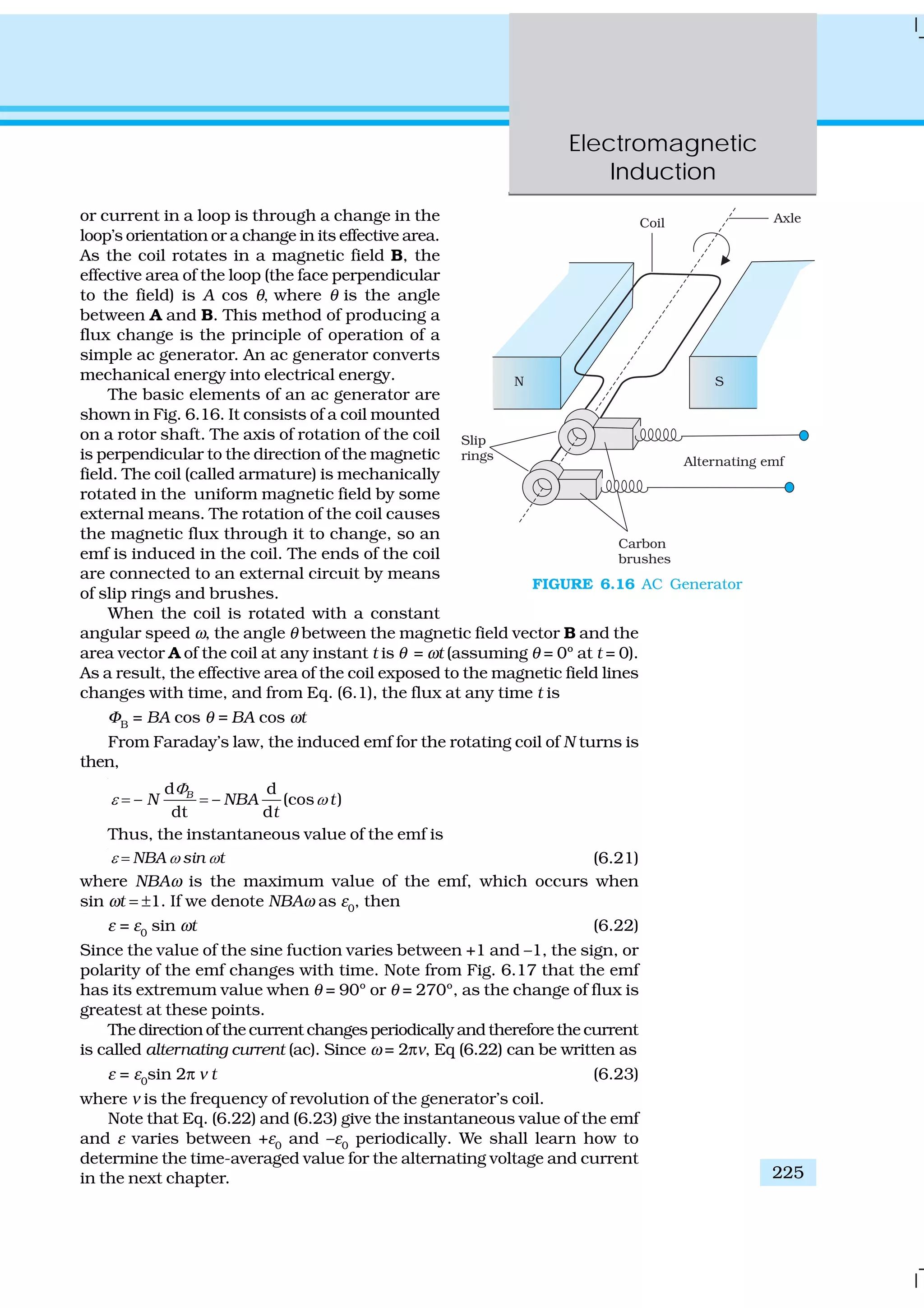
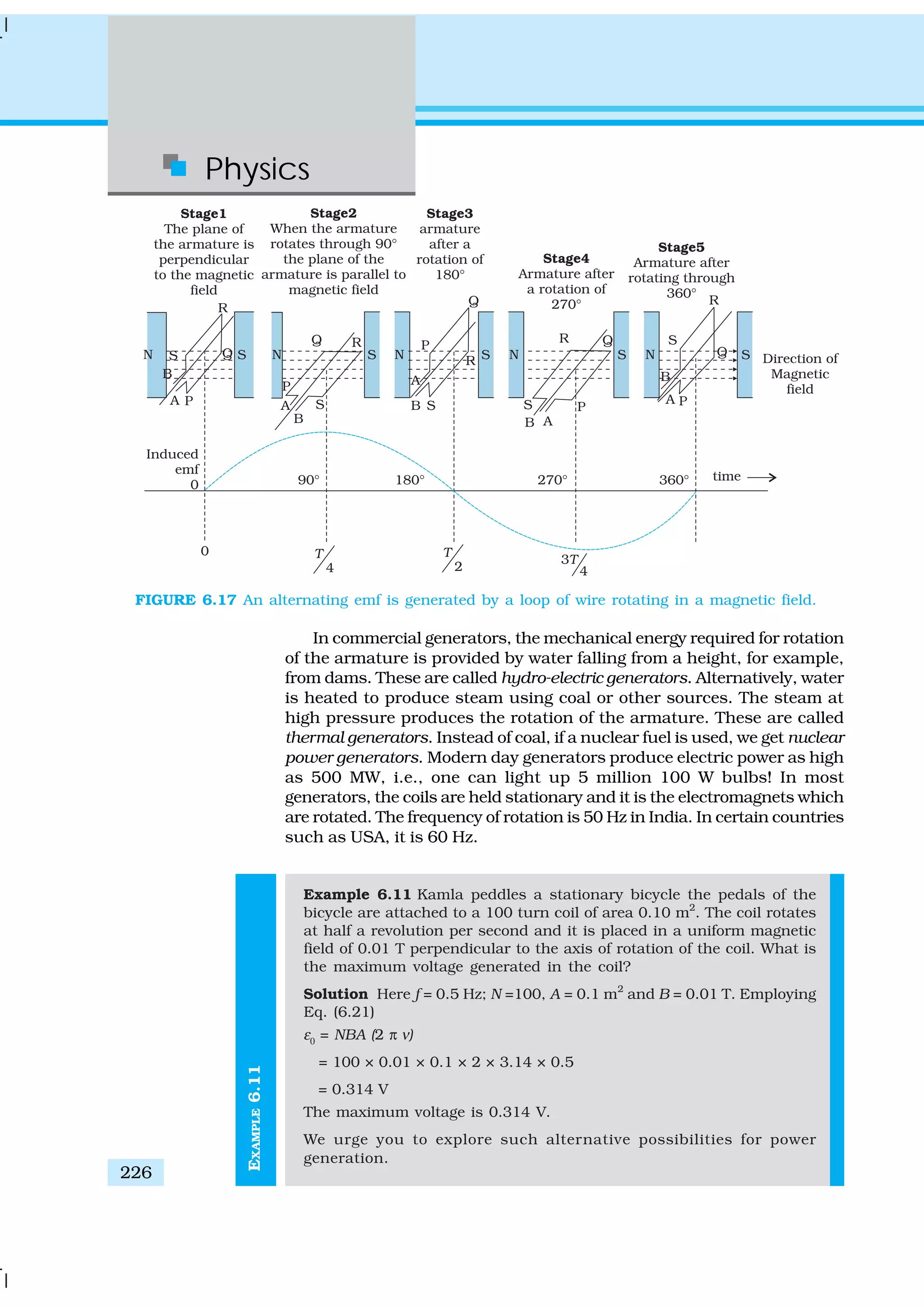
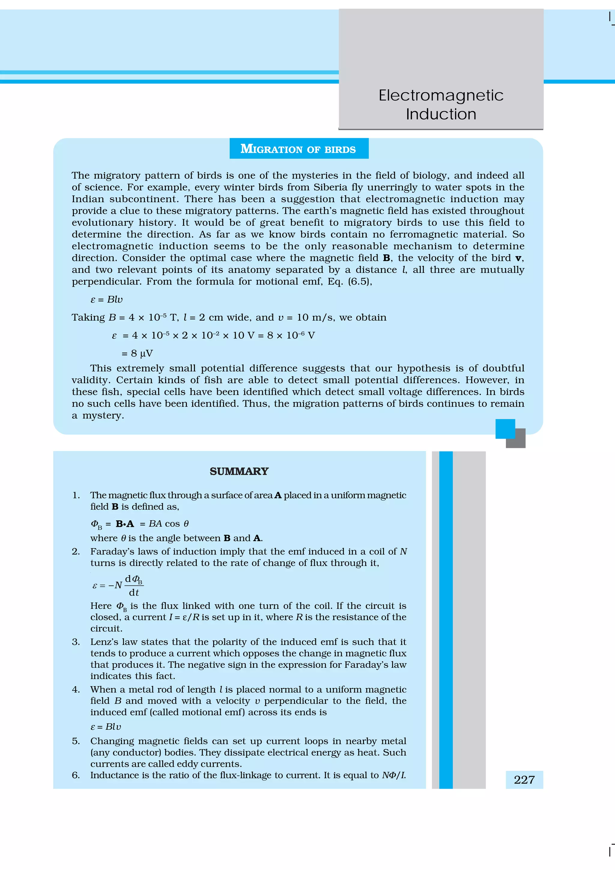
232. Physics
228
POINTS TO PONDER
1. Electricity and magnetism are intimately related. In the early part of the
nineteenth century, the experiments of Oersted, Ampere and others
established that moving charges (currents) produce a magnetic field.
Somewhat later, around 1830, the experiments of Faraday and Henry
demonstrated that a moving magnet can induce electric current.
2. In a closed circuit, electric currents are induced so as to oppose the
changing magnetic flux. It is as per the law of conservation of energy.
However, in case of an open circuit, an emf is induced across its ends.
How is it related to the flux change?
3. The motional emf discussed in Section 6.5 can be argued independently
from Faraday’s law using the Lorentz force on moving charges. However,
Quantity Symbol Units Dimensions Equations
Magnetic Flux ΦB
Wb (weber) [M L2
T–2
A–1
] ΦB
= B Ai
EMF ε V (volt) [M L2
T–3
A–1
] ε = Bd( )/dN tΦ−
Mutual Inductance M H (henry) [M L2
T–2
A–2
] ε1
( )12 2d /dM I t= −
Self Inductance L H (henry) [M L2
T–2
A–2
] ( )d /dL I tε = −
7. A changing current in a coil (coil 2) can induce an emf in a nearby coil
(coil 1). This relation is given by,
2
1 12
d
d
I
M
t
ε = −
The quantity M12
is called mutual inductance of coil 1 with respect to
coil 2. One can similarly define M21
. There exists a general equality,
M12
= M21
8. When a current in a coil changes, it induces a back emf in the same
coil. The self-induced emf is given by,
d
d
I
L
t
ε = −
L is the self-inductance of the coil. It is a measure of the inertia of the
coil against the change of current through it.
9. The self-inductance of a long solenoid, the core of which consists of a
magnetic material of permeability μr
, is given by
L = μr
μ0
n2
Al
where A is the area of cross-section of the solenoid, l its length and n
the number of turns per unit length.
10. In an ac generator, mechanical energy is converted to electrical energy
by virtue of electromagnetic induction. If coil of N turn and area A is
rotated at ν revolutions per second in a uniform magnetic field B, then
the motional emf produced is
ε = NBA (2πν) sin (2πνt)
where we have assumed that at time t = 0 s, the coil is perpendicular to
the field.

233. Electromagnetic
Induction
229
EXERCISES
6.1 Predict the direction of induced current in the situations described
by the following Figs. 6.18(a) to (f ).
even if the charges are stationary [and the q (v × B) term of the Lorentz
force is not operative], an emf is nevertheless induced in the presence of a
time-varying magnetic field. Thus, moving charges in static field and static
charges in a time-varying field seem to be symmetric situation for
Faraday’s law. This gives a tantalising hint on the relevance of the principle
of relativity for Faraday’s law.
4. The motion of a copper plate is damped when it is allowed to oscillate
between the magnetic pole-pieces. How is the damping force, produced by
the eddy currents?
FIGURE 6.18

234. Physics
230
6.2 Use Lenz’s law to determine the direction of induced current in the
situations described by Fig. 6.19:
(a) A wire of irregular shape turning into a circular shape;
(b) A circular loop being deformed into a narrow straight wire.
FIGURE 6.19
6.3 A long solenoid with 15 turns per cm has a small loop of area 2.0 cm2
placed inside the solenoid normal to its axis. If the current carried
by the solenoid changes steadily from 2.0 A to 4.0 A in 0.1 s, what is
the induced emf in the loop while the current is changing?
6.4 A rectangular wire loop of sides 8 cm and 2 cm with a small cut is
moving out of a region of uniform magnetic field of magnitude 0.3 T
directed normal to the loop. What is the emf developed across the
cut if the velocity of the loop is 1 cm s–1
in a direction normal to the
(a) longer side, (b) shorter side of the loop? For how long does the
induced voltage last in each case?
6.5 A 1.0 m long metallic rod is rotated with an angular frequency of
400 rad s–1
about an axis normal to the rod passing through its one
end. The other end of the rod is in contact with a circular metallic
ring. A constant and uniform magnetic field of 0.5 T parallel to the
axis exists everywhere. Calculate the emf developed between the
centre and the ring.
6.6 A circular coil of radius 8.0 cm and 20 turns is rotated about its
vertical diameter with an angular speed of 50 rad s–1
in a uniform
horizontal magnetic field of magnitude 3.0 × 10–2
T. Obtain the
maximum and average emf induced in the coil. If the coil forms a
closed loop of resistance 10 Ω, calculate the maximum value of current
in the coil. Calculate the average power loss due to Joule heating.
Where does this power come from?
6.7 A horizontal straight wire 10 m long extending from east to west is
falling with a speed of 5.0 m s–1
, at right angles to the horizontal
component of the earth’s magnetic field, 0.30 × 10–4
Wb m–2
.
(a) What is the instantaneous value of the emf induced in the wire?
(b) What is the direction of the emf?
(c) Which end of the wire is at the higher electrical potential?
6.8 Current in a circuit falls from 5.0 A to 0.0 A in 0.1 s. If an average emf
of 200 V induced, give an estimate of the self-inductance of the circuit.
6.9 A pair of adjacent coils has a mutual inductance of 1.5 H. If the
current in one coil changes from 0 to 20 A in 0.5 s, what is the
change of flux linkage with the other coil?
6.10 A jet plane is travelling towards west at a speed of 1800 km/h. What
is the voltage difference developed between the ends of the wing

235. Electromagnetic
Induction
231
having a span of 25 m, if the Earth’s magnetic field at the location
has a magnitude of 5 × 10–4
T and the dip angle is 30°.
ADDITIONAL EXERCISES
6.11 Suppose the loop in Exercise 6.4 is stationary but the current
feeding the electromagnet that produces the magnetic field is
gradually reduced so that the field decreases from its initial value
of 0.3 T at the rate of 0.02 T s–1
. If the cut is joined and the loop
has a resistance of 1.6 Ω, how much power is dissipated by the
loop as heat? What is the source of this power?
6.12 A square loop of side 12 cm with its sides parallel to X and Y axes is
moved with a velocity of 8 cm s–1
in the positive x-direction in an
environment containing a magnetic field in the positive z-direction.
The field is neither uniform in space nor constant in time. It has a
gradient of 10 – 3
T cm–1
along the negative x-direction (that is it increases
by 10 – 3
T cm –1
as one moves in the negative x-direction), and it is
decreasing in time at the rate of 10–3
T s–1
. Determine the direction and
magnitude of the induced current in the loop if its resistance is 4.50 mΩ.
6.13 It is desired to measure the magnitude of field between the poles of a
powerful loud speaker magnet. A small flat search coil of area 2 cm2
with 25 closely wound turns, is positioned normal to the field
direction, and then quickly snatched out of the field region.
Equivalently, one can give it a quick 90° turn to bring its plane
parallel to the field direction). The total charge flown in the coil
(measured by a ballistic galvanometer connected to coil) is
7.5 mC. The combined resistance of the coil and the galvanometer is
0.50 Ω. Estimate the field strength of magnet.
6.14 Figure 6.20 shows a metal rod PQ resting on the smooth rails AB
and positioned between the poles of a permanent magnet. The rails,
the rod, and the magnetic field are in three mutual perpendicular
directions. A galvanometer G connects the rails through a switch K.
Length of the rod = 15 cm, B = 0.50 T, resistance of the closed loop
containing the rod = 9.0 mΩ. Assume the field to be uniform.
(a) Suppose K is open and the rod is moved with a speed of 12 cm s–1
in the direction shown. Give the polarity and magnitude of the
induced emf.
FIGURE 6.20
(b) Is there an excess charge built up at the ends of the rods when
K is open? What if K is closed?
(c) With K open and the rod moving uniformly, there is no net
force on the electrons in the rod PQ even though they do

236. Physics
232
experience magnetic force due to the motion of the rod. Explain.
(d) What is the retarding force on the rod when K is closed?
(e) How much power is required (by an external agent) to keep
the rod moving at the same speed (=12 cm s–1
) when K is closed?
How much power is required when K is open?
(f ) How much power is dissipated as heat in the closed circuit?
What is the source of this power?
(g) What is the induced emf in the moving rod if the magnetic field
is parallel to the rails instead of being perpendicular?
6.15 An air-cored solenoid with length 30 cm, area of cross-section 25 cm2
and number of turns 500, carries a current of 2.5 A. The current is
suddenly switched off in a brief time of 10–3
s. How much is the average
back emf induced across the ends of the open switch in the circuit?
Ignore the variation in magnetic field near the ends of the solenoid.
6.16 (a) Obtain an expression for the mutual inductance between a long
straight wire and a square loop of side a as shown in Fig. 6.21.
(b) Now assume that the straight wire carries a current of 50 A and
the loop is moved to the right with a constant velocity, v = 10 m/s.
Calculate the induced emf in the loop at the instant when x = 0.2 m.
Take a = 0.1 m and assume that the loop has a large resistance.
FIGURE 6.21
6.17 A line charge λ per unit length is lodged uniformly onto the rim of a
wheel of mass M and radius R. The wheel has light non-conducting
spokes and is free to rotate without friction about its axis (Fig. 6.22).
A uniform magnetic field extends over a circular region within the
rim. It is given by,
B = – B0
k (r ≤ a; a < R)
= 0 (otherwise)
What is the angular velocity of the wheel after the field is suddenly
switched off?
FIGURE 6.22

237. 7.1 INTRODUCTION
We have so far considered direct current (dc) sources and circuits with dc
sources. These currents do not change direction with time. But voltages
and currents that vary with time are very common. The electric mains
supply in our homes and offices is a voltage that varies like a sine function
with time. Such a voltage is called alternating voltage (ac voltage) and
the current driven by it in a circuit is called the alternating current (ac
current)*. Today, most of the electrical devices we use require ac voltage.
This is mainly because most of the electrical energy sold by power
companies is transmitted and distributed as alternating current. The main
reason for preferring use of ac voltage over dc voltage is that ac voltages
can be easily and efficiently converted from one voltage to the other by
means of transformers. Further, electrical energy can also be transmitted
economically over long distances. AC circuits exhibit characteristics which
are exploited in many devices of daily use. For example, whenever we
tune our radio to a favourite station, we are taking advantage of a special
property of ac circuits – one of many that you will study in this chapter.
Chapter Seven
ALTERNATING
CURRENT
* The phrases ac voltage and ac current are contradictory and redundant,
respectively, since they mean, literally, alternating current voltage and alternating
current current. Still, the abbreviation ac to designate an electrical quantity
displaying simple harmonic time dependance has become so universally accepted
that we follow others in its use. Further, voltage – another phrase commonly
used means potential difference between two points.

238. Physics
234
NICOLATESLA(1836–1943)
Nicola Tesla (1836 –
1943) Yugoslov scientist,
inventor and genius. He
conceived the idea of the
rotating magnetic field,
which is the basis of
practically all alternating
current machinery, and
which helped usher in the
age of electric power. He
also invented among other
things the induction motor,
the polyphase system of ac
power, and the high
frequency induction coil
(the Tesla coil) used in radio
and television sets and
other electronic equipment.
The SI unit of magnetic field
is named in his honour.
7.2 AC VOLTAGE APPLIED TO A RESISTOR
Figure 7.1 shows a resistor connected to a source ε of
ac voltage. The symbol for an ac source in a circuit
diagram is ~ . We consider a source which produces
sinusoidally varying potential difference across its
terminals. Let this potential difference, also called ac
voltage, be given by
sinmv v tω= (7.1)
where vm
is the amplitude of the oscillating potential
difference and ω is its angular frequency.
To find the value of current through the resistor, we
apply Kirchhoff’s loop rule ( ) 0ε =∑ t , to the circuit
shown in Fig. 7.1 to get
=sinmv t i Rω
or sinmv
i t
R
ω=
Since R is a constant, we can write this equation as
sinmi i tω= (7.2)
where the current amplitude im
is given by
m
m
v
i
R
= (7.3)
Equation (7.3) is just Ohm’s law which for resistors works
equally well for both ac and dc voltages. The voltage across a
pure resistor and the current through it, given by Eqs. (7.1) and
(7.2) are plotted as a function of time in Fig. 7.2. Note, in
particular that both v and i reach zero, minimum and maximum
values at the same time. Clearly, the voltage and current are in
phase with each other.
We see that, like the applied voltage, the current varies
sinusoidally and has corresponding positive and negative values
during each cycle. Thus, the sum of the instantaneous current
values over one complete cycle is zero, and the average current
is zero. The fact that the average current is zero, however, does
FIGURE 7.1 AC voltage applied to a resistor.
FIGURE 7.2 In a pure
resistor, the voltage and
current are in phase. The
minima, zero and maxima
occur at the same
respective times.

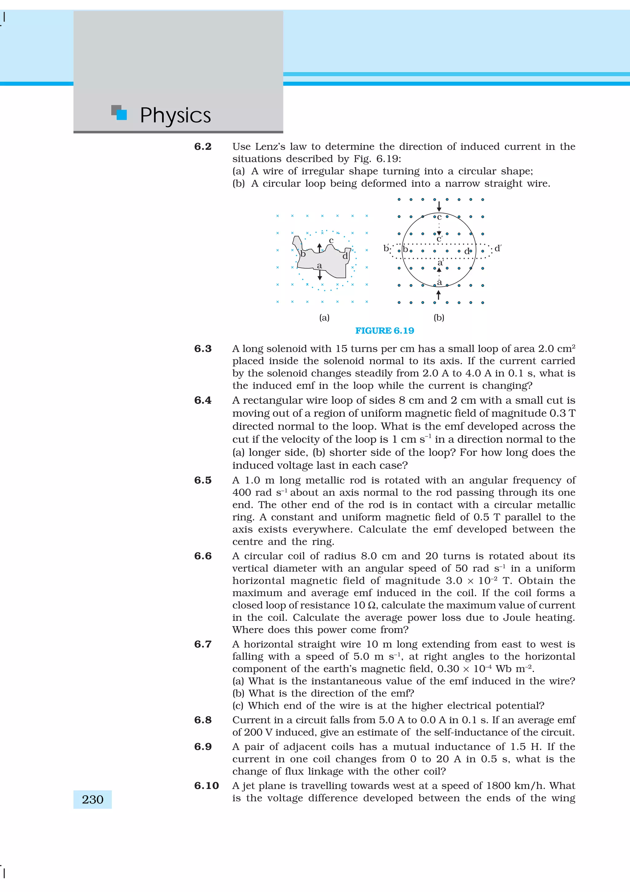
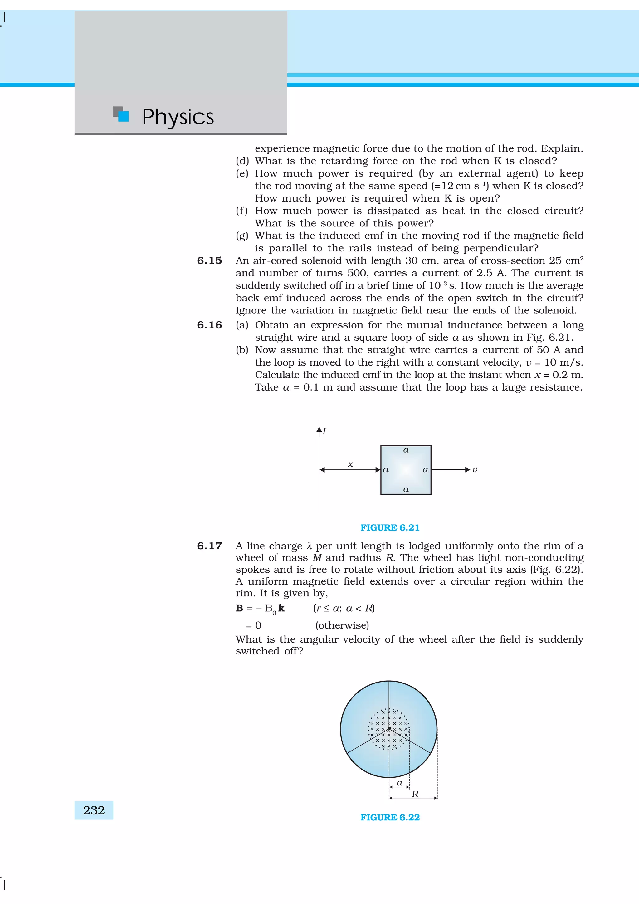
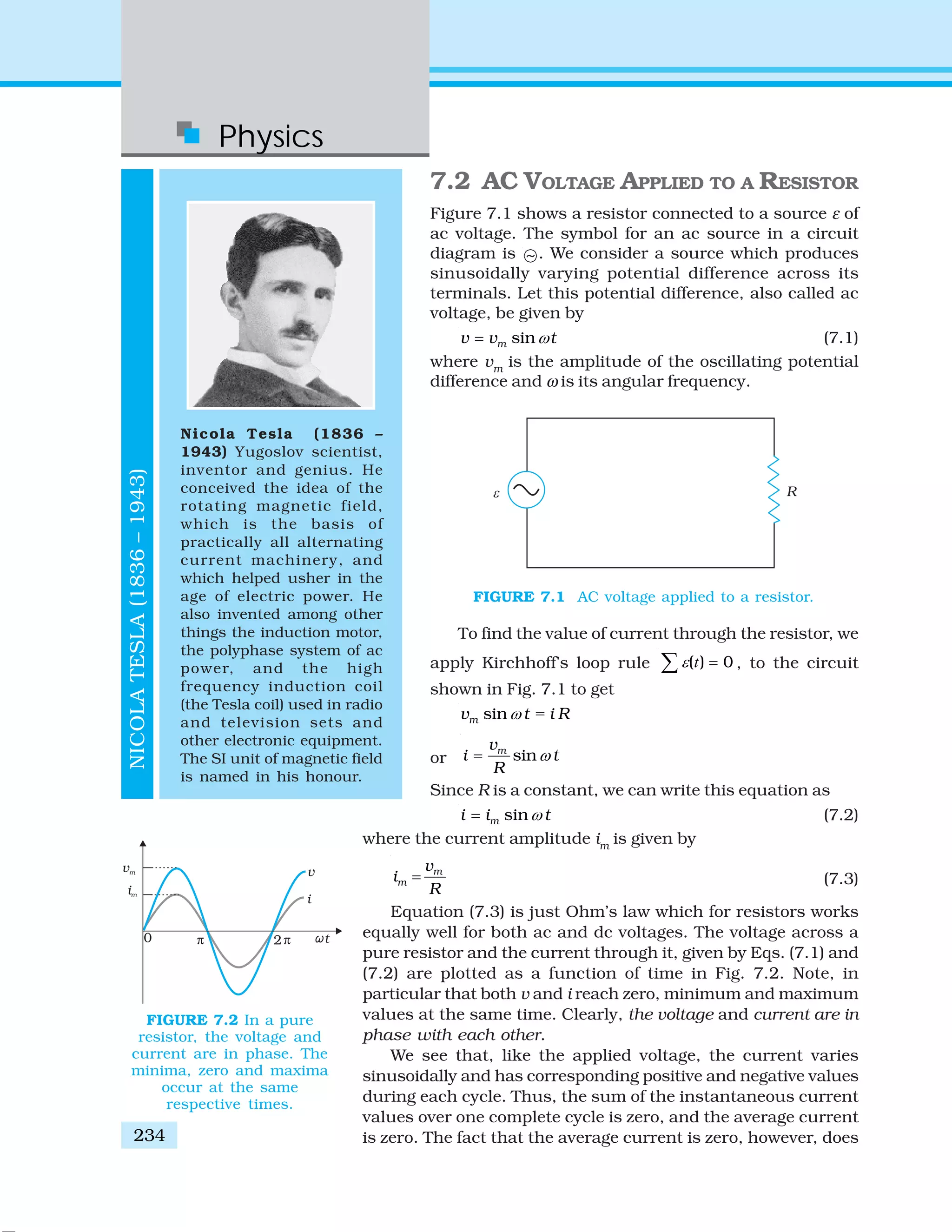
239. Alternating Current
235
GEORGEWESTINGHOUSE(1846–1914)
George Westinghouse
(1846 – 1914) A leading
proponent of the use of
alternating current over
direct current. Thus,
he came into conflict
with Thomas Alva Edison,
an advocate of direct
current. Westinghouse
was convinced that the
technology of alternating
current was the key to
the electrical future.
He founded the famous
Company named after him
and enlisted the services
of Nicola Tesla and
other inventors in the
development of alternating
current motors and
apparatus for the
transmission of high
tension current, pioneering
in large scale lighting.
not mean that the average power consumed is zero and
that there is no dissipation of electrical energy. As you
know, Joule heating is given by i2
R and depends on i2
(which is always positive whether i is positive or negative)
and not on i. Thus, there is Joule heating and
dissipation of electrical energy when an
ac current passes through a resistor.
The instantaneous power dissipated in the resistor is
2 2 2
sinmp i R i R tω= = (7.4)
The average value of p over a cycle is*
2 2 2
sinmp i R i R tω= < > = < > [7.5(a)]
where the bar over a letter(here, p) denotes its average
value and <......> denotes taking average of the quantity
inside the bracket. Since, i2
m
and R are constants,
2 2
sinmp i R tω= < > [7.5(b)]
Using the trigonometric identity, sin2
ωt =
1/2 (1– cos 2ωt), we have < sin2
ωt > = (1/2) (1– < cos 2ωt >)
and since < cos2ωt > = 0**, we have,
2 1
sin
2
tω< > =
Thus,
21
2
mp i R= [7.5(c)]
To express ac power in the same form as dc power
(P = I2
R), a special value of current is defined and used.
It is called, root mean square (rms) or effective current
(Fig. 7.3) and is denoted by Irms
or I.
* The average value of a function F (t) over a period T is given by d
0
1
( ) ( )
T
F t F t t
T
= ∫
** [ ]
0 0
sin 21 1 1
cos2 cos2 sin 2 0 0
2 2
TT
t
t t dt T
T T T
ω
ω ω ω
ω ω
⎡ ⎤
< > = = = − =∫ ⎢ ⎥⎣ ⎦
FIGURE 7.3 The rms current I is related to the
peak current im
by I = / 2mi = 0.707 im
.

240. Physics
236
It is defined by
2 21
2 2
m
m
i
I i i= = =
= 0.707 im
(7.6)
In terms of I, the average power, denoted by P is
2 21
2
m
pP i R I R= = = (7.7)
Similarly, we define the rms voltage or effective voltage by
V =
2
mv
= 0.707 vm
(7.8)
From Eq. (7.3), we have
vm
= im
R
or,
2 2
m mv i
R=
or, V = IR (7.9)
Equation (7.9) gives the relation between ac current and ac voltage
and is similar to that in the dc case. This shows the advantage of
introducing the concept of rms values. In terms of rms values, the equation
for power [Eq. (7.7)] and relation between current and voltage in ac circuits
are essentially the same as those for the dc case.
It is customary to measure and specify rms values for ac quantities. For
example, the household line voltage of 220 V is an rms value with a peak
voltage of
vm
= 2 V = (1.414)(220 V) = 311 V
In fact, the I or rms current is the equivalent dc current that would
produce the same average power loss as the alternating current. Equation
(7.7) can also be written as
P = V2
/ R = I V (since V = I R)
Example 7.1 A light bulb is rated at 100W for a 220 V supply. Find
(a) the resistance of the bulb; (b) the peak voltage of the source; and
(c) the rms current through the bulb.
Solution
(a) We are given P = 100 W and V = 220 V. The resistance of the
bulb is
( )
2
2
220 V
484
100 W
V
R
P
= = = Ω
(b) The peak voltage of the source is
V2 311m
v V= =
(c) Since, P = I V
100 W
0.450A
220 V
P
I
V
= = =
EXAMPLE7.1

241. Alternating Current
237
7.3 REPRESENTATION OF AC CURRENT AND VOLTAGE
BY ROTATING VECTORS — PHASORS
In the previous section, we learnt that the current through a resistor is
in phase with the ac voltage. But this is not so in the case of an inductor,
a capacitor or a combination of these circuit elements. In order to show
phase relationship between voltage and current
in an ac circuit, we use the notion of phasors.
The analysis of an ac circuit is facilitated by the
use of a phasor diagram. A phasor* is a vector
which rotates about the origin with angular
speed ω, as shown in Fig. 7.4. The vertical
components of phasors V and I represent the
sinusoidally varying quantities v and i. The
magnitudes of phasors V and I represent the
amplitudes or the peak values vm
and im
of these
oscillating quantities. Figure 7.4(a) shows the
voltage and current phasors and their
relationship at time t1
for the case of an ac source
connected to a resistor i.e., corresponding to the
circuit shown in Fig. 7.1. The projection of
voltage and current phasors on vertical axis, i.e., vm
sinωt and im
sinωt,
respectively represent the value of voltage and current at that instant. As
they rotate with frequency ω, curves in Fig. 7.4(b) are generated.
From Fig. 7.4(a) we see that phasors V and I for the case of a resistor are
in the same direction. This is so for all times. This means that the phase
angle between the voltage and the current is zero.
7.4 AC VOLTAGE APPLIED TO AN INDUCTOR
Figure 7.5 shows an ac source connected to an inductor. Usually,
inductors have appreciable resistance in their windings, but we shall
assume that this inductor has negligible resistance.
Thus, the circuit is a purely inductive ac circuit. Let
the voltage across the source be v = vm
sinωt. Using
the Kirchhoff’s loop rule, ( ) 0tε =∑ , and since there
is no resistor in the circuit,
d
0
d
i
v L
t
− = (7.10)
where the second term is the self-induced Faraday
emf in the inductor; and L is the self-inductance of
FIGURE 7.4 (a) A phasor diagram for the
circuit in Fig 7.1. (b) Graph of v and
i versus ωt.
FIGURE 7.5 An ac source
connected to an inductor.
* Though voltage and current in ac circuit are represented by phasors – rotating
vectors, they are not vectors themselves. They are scalar quantities. It so happens
that the amplitudes and phases of harmonically varying scalars combine
mathematically in the same way as do the projections of rotating vectors of
corresponding magnitudes and directions. The rotating vectors that represent
harmonically varying scalar quantities are introduced only to provide us with a
simple way of adding these quantities using a rule that we already know.

242. Physics
238
the inductor. The negative sign follows from Lenz’s law (Chapter 6).
Combining Eqs. (7.1) and (7.10), we have
d
sin
d
mvi v
t
t L L
ω= = (7.11)
Equation (7.11) implies that the equation for i(t), the current as a
function of time, must be such that its slope di/dt is a sinusoidally varying
quantity, with the same phase as the source voltage and an amplitude
given by vm
/L. To obtain the current, we integrate di/dt with respect to
time:
d
d sin( )d
d
mvi
t t t
t L
ω=∫ ∫
and get,
cos( ) constantmv
i t
L
= − ω +
ω
The integration constant has the dimension of current and is time-
independent. Since the source has an emf which oscillates symmetrically
about zero, the current it sustains also oscillates symmetrically about
zero, so that no constant or time-independent component of the current
exists. Therefore, the integration constant is zero.
Using
cos( ) sin
2
t tω ω
π⎛ ⎞
− = −⎜ ⎟⎝ ⎠ , we have
sin
2
mi i tω
π⎛ ⎞
= −⎜ ⎟⎝ ⎠ (7.12)
where
m
m
v
i
L
=
ω
is the amplitude of the current. The quantity ω L is
analogous to the resistance and is called inductive reactance, denoted
by XL
:
XL
= ω L (7.13)
The amplitude of the current is, then
m
m
L
v
i
X
= (7.14)
The dimension of inductive reactance is the same as that of resistance
and its SI unit is ohm (Ω). The inductive reactance limits the current in a
purely inductive circuit in the same way as the resistance limits the
current in a purely resistive circuit. The inductive reactance is directly
proportional to the inductance and to the frequency of the current.
A comparison of Eqs. (7.1) and (7.12) for the source voltage and the
current in an inductor shows that the current lags the voltage by π/2 or
one-quarter (1/4) cycle. Figure 7.6 (a) shows the voltage and the current
phasors in the present case at instant t1
. The current phasor I is π/2
behind the voltage phasor V. When rotated with frequency ω counter-
clockwise, they generate the voltage and current given by Eqs. (7.1) and
(7.12), respectively and as shown in Fig. 7.6(b).
InteractiveanimationonPhasordiagramsofaccircuitscontaining,R,L,CandRLCseriescircuits:
http://www.phys.unsw.edu.au/~jw/AC.html

243. Alternating Current
239
EXAMPLE7.2
We see that the current reaches its maximum value later than the
voltage by one-fourth of a period
/2
4
T
ω
π⎡ ⎤
=⎢ ⎥⎣ ⎦
. You have seen that an
inductor has reactance that limits current similar to resistance in a
dc circuit. Does it also consume power like a resistance? Let us try to
find out.
The instantaneous power supplied to the inductor is
( )sin × sin
2
L m mp i v i t v tω ω
π⎛ ⎞
= = −⎜ ⎟⎝ ⎠
( ) ( )cos sinm mi v t tω ω= −
( )sin 2
2
m mi v
tω= −
So, the average power over a complete cycle is
( )L sin 2
2
m mi v
P tω= −
( )sin 2
2
m mi v
tω= − = 0,
since the average of sin (2ωt) over a complete cycle is zero.
Thus, the average power supplied to an inductor over one complete
cycle is zero.
Figure 7.7 explains it in detail.
Example 7.2 A pure inductor of 25.0 mH is connected to a source of
220 V. Find the inductive reactance and rms current in the circuit if
the frequency of the source is 50 Hz.
Solution The inductive reactance,
–
= . 3
2 2 3 14 50 25 10 WLX Lνπ × × × ×=
= 7.85Ω
The rms current in the circuit is
V
A
220
28
7.85L
V
I
X
= = =
Ω
FIGURE 7.6 (a) A Phasor diagram for the circuit in Fig. 7.5.
(b) Graph of v and i versus ωt.

244. Physics
240
0-1 Current i through the coil entering at A
increase from zero to a maximum value. Flux
lines are set up i.e., the core gets magnetised.
With the polarity shown voltage and current
are both positive. So their product p is positive.
ENERGY IS ABSORBED FROM THE
SOURCE.
1-2 Current in the coil is still positive but is
decreasing. The core gets demagnetised and
the net flux becomes zero at the end of a half
cycle. The voltage v is negative (since di/dt is
negative). The product of voltage and current
is negative, and ENERGY IS BEING
RETURNED TO SOURCE.
One complete cycle of voltage/current. Note that the current lags the voltage.
2-3 Current i becomes negative i.e., it enters
at B and comes out of A. Since the direction
of current has changed, the polarity of the
magnet changes. The current and voltage are
both negative. So their product p is positive.
ENERGY IS ABSORBED.
3-4 Current i decreases and reaches its zero
value at 4 when core is demagnetised and flux
is zero. The voltage is positive but the current
is negative. The power is, therefore, negative.
ENERGY ABSORBED DURING THE 1/4
CYCLE 2-3 IS RETURNED TO THE SOURCE.
FIGURE 7.7 Magnetisation and demagnetisation of an inductor.

245. Alternating Current
241
7.5 AC VOLTAGE APPLIED TO A CAPACITOR
Figure 7.8 shows an ac source ε generating ac voltage v = vm
sin ωt
connected to a capacitor only, a purely capacitive ac circuit.
When a capacitor is connected to a voltage source
in a dc circuit, current will flow for the short time
required to charge the capacitor. As charge
accumulates on the capacitor plates, the voltage
across them increases, opposing the current. That is,
a capacitor in a dc circuit will limit or oppose the
current as it charges. When the capacitor is fully
charged, the current in the circuit falls to zero.
When the capacitor is connected to an ac source,
as in Fig. 7.8, it limits or regulates the current, but
does not completely prevent the flow of charge. The
capacitor is alternately charged and discharged as
the current reverses each half cycle. Let q be the
charge on the capacitor at any time t. The instantaneous voltage v across
the capacitor is
q
v
C
= (7.15)
From the Kirchhoff’s loop rule, the voltage across the source and the
capacitor are equal,
sinm
q
v t
C
ω =
To find the current, we use the relation
d
d
q
i
t
=
( )
d
d
sin cos( )m mi v C t C v t
t
ω ω ω= =
Using the relation, cos( ) sin
2
t tω ω
π⎛ ⎞
= +⎜ ⎟⎝ ⎠
, we have
sin
2
mi i tω
π⎛ ⎞
= +⎜ ⎟⎝ ⎠ (7.16)
where the amplitude of the oscillating current is im
= ωCvm
. We can rewrite
it as
(1/ )
m
m
v
i
Cω
=
Comparing it to im
= vm
/R for a purely resistive circuit, we find that
(1/ωC) plays the role of resistance. It is called capacitive reactance and
is denoted by Xc
,
Xc
= 1/ωC (7.17)
so that the amplitude of the current is
m
m
C
v
i
X
= (7.18)
FIGURE 7.8 An ac source
connected to a capacitor.

246. Physics
242
FIGURE 7.9 (a) A Phasor diagram for the circuit
in Fig. 7.8. (b) Graph of v and i versus ωt.
The dimension of capacitive reactance is the
same as that of resistance and its SI unit is
ohm (Ω). The capacitive reactance limits the
amplitude of the current in a purely capacitive
circuit in the same way as the resistance limits
the current in a purely resistive circuit. But it
is inversely proportional to the frequency and
the capacitance.
A comparison of Eq. (7.16) with the
equation of source voltage, Eq. (7.1) shows that
the current is π/2 ahead of voltage.
Figure 7.9(a) shows the phasor diagram at an instant t1
. Here the current
phasor I is π/2 ahead of the voltage phasor V as they rotate
counterclockwise. Figure 7.9(b) shows the variation of voltage and current
with time. We see that the current reaches its maximum value earlier than
the voltage by one-fourth of a period.
The instantaneous power supplied to the capacitor is
pc
= i v = im
cos(ωt)vm
sin(ωt)
= im
vm
cos(ωt) sin(ωt)
sin(2 )
2
m mi v
tω= (7.19)
So, as in the case of an inductor, the average power
sin(2 ) sin(2 ) 0
2 2
m m m m
C
i v i v
P t tω ω= = =
since <sin (2ωt)> = 0 over a complete cycle. Figure 7.10 explains it in detail.
Thus, we see that in the case of an inductor, the current lags the voltage
by π/2 and in the case of a capacitor, the current leads the voltage by π/2.
Example 7.3 A lamp is connected in series with a capacitor. Predict
your observations for dc and ac connections. What happens in each
case if the capacitance of the capacitor is reduced?
Solution When a dc source is connected to a capacitor, the capacitor
gets charged and after charging no current flows in the circuit and
the lamp will not glow. There will be no change even if C is reduced.
With ac source, the capacitor offers capacitative reactance (1/ωC )
and the current flows in the circuit. Consequently, the lamp will shine.
Reducing C will increase reactance and the lamp will shine less brightly
than before.
Example 7.4 A 15.0 μF capacitor is connected to a 220 V, 50 Hz source.
Find the capacitive reactance and the current (rms and peak) in the
circuit. If the frequency is doubled, what happens to the capacitive
reactance and the current?
Solution The capacitive reactance is
F6
1 1
212
2 2 (50Hz)(15.0 10 )
CX
Cν −
= = = Ω
π π ×
The rms current is
EXAMPLE7.4EXAMPLE7.3

247. Alternating Current
243
0-1 The current i flows as shown and from the
maximum at 0, reaches a zero value at 1. The plate
A is charged to positive polarity while negative charge
q builds up in B reaching a maximum at 1 until the
current becomes zero. The voltage vc = q/C is in phase
with q and reaches maximum value at 1. Current
and voltage are both positive. So p = vci is positive.
ENERGY IS ABSORBED FROM THE SOURCE
DURING THIS QUAR TER CYCLE AS THE
CAPACITOR IS CHARGED.
1-2 The current i reverses its direction. The
accumulated charge is depleted i.e., the capacitor is
discharged during this quarter cycle.The voltage gets
reduced but is still positive. The current is negative.
Their product, the power is negative.
THE ENERGY ABSORBED DURING THE 1/4
CYCLE 0-1 IS RETURNED DURING THIS QUARTER.
One complete cycle of voltage/current. Note that the current leads the voltage.
2-3 As i continues to flow from A to B, the capacitor
is charged to reversed polarity i.e., the plate B
acquires positive and A acquires negative charge.
Both the current and the voltage are negative. Their
product p is positive. The capacitor ABSORBS
ENERGY during this 1/4 cycle.
3-4 The current i reverses its direction at 3 and flows
from B to A. The accumulated charge is depleted
and the magnitude of the voltage vc is reduced. vc
becomes zero at 4 when the capacitor is fully
discharged. The power is negative.ENERGY
ABSORBED DURING 2-3 IS RETURNED TO THE
SOURCE. NET ENERGY ABSORBED IS ZERO.
FIGURE 7.10 Charging and discharging of a capacitor.

248. Physics
244
EXAMPLE7.5EXAMPLE7.4
V
A
220
1.04
212C
V
I
X
= = =
Ω
The peak current is
2 (1.41)(1.04 ) 1.47mi I A A= = =
This current oscillates between +1.47A and –1.47 A, and is ahead of
the voltage by π/2.
If the frequency is doubled, the capacitive reactance is halved and
consequently, the current is doubled.
Example 7.5 A light bulb and an open coil inductor are connected to
an ac source through a key as shown in Fig. 7.11.
FIGURE 7.11
The switch is closed and after sometime, an iron rod is inserted into
the interior of the inductor. The glow of the light bulb (a) increases; (b)
decreases; (c) is unchanged, as the iron rod is inserted. Give your
answer with reasons.
Solution As the iron rod is inserted, the magnetic field inside the coil
magnetizes the iron increasing the magnetic field inside it. Hence,
the inductance of the coil increases. Consequently, the inductive
reactance of the coil increases. As a result, a larger fraction of the
applied ac voltage appears across the inductor, leaving less voltage
across the bulb. Therefore, the glow of the light bulb decreases.
7.6 AC VOLTAGE APPLIED TO A SERIES LCR CIRCUIT
Figure 7.12 shows a series LCR circuit connected to an ac source ε. As
usual, we take the voltage of the source to be v = vm
sin ωt.
If q is the charge on the capacitor and i the
current, at time t, we have, from Kirchhoff’s loop
rule:
d
d
i q
L i R v
t C
+ + = (7.20)
We want to determine the instantaneous
current i and its phase relationship to the applied
alternating voltage v. We shall solve this problem
by two methods. First, we use the technique of
phasors and in the second method, we solve
Eq. (7.20) analytically to obtain the time–
dependence of i.
FIGURE 7.12 A series LCR circuit
connected to an ac source.

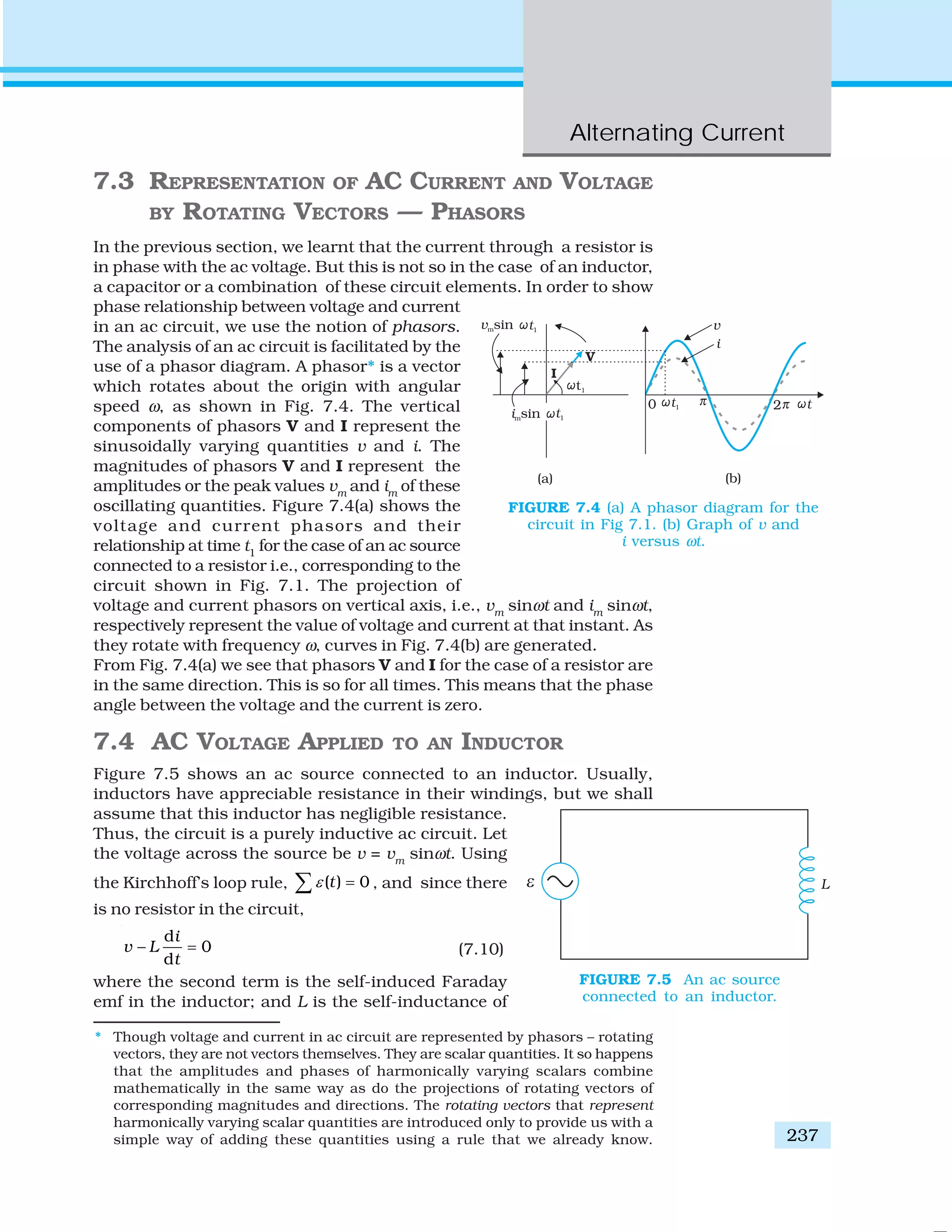
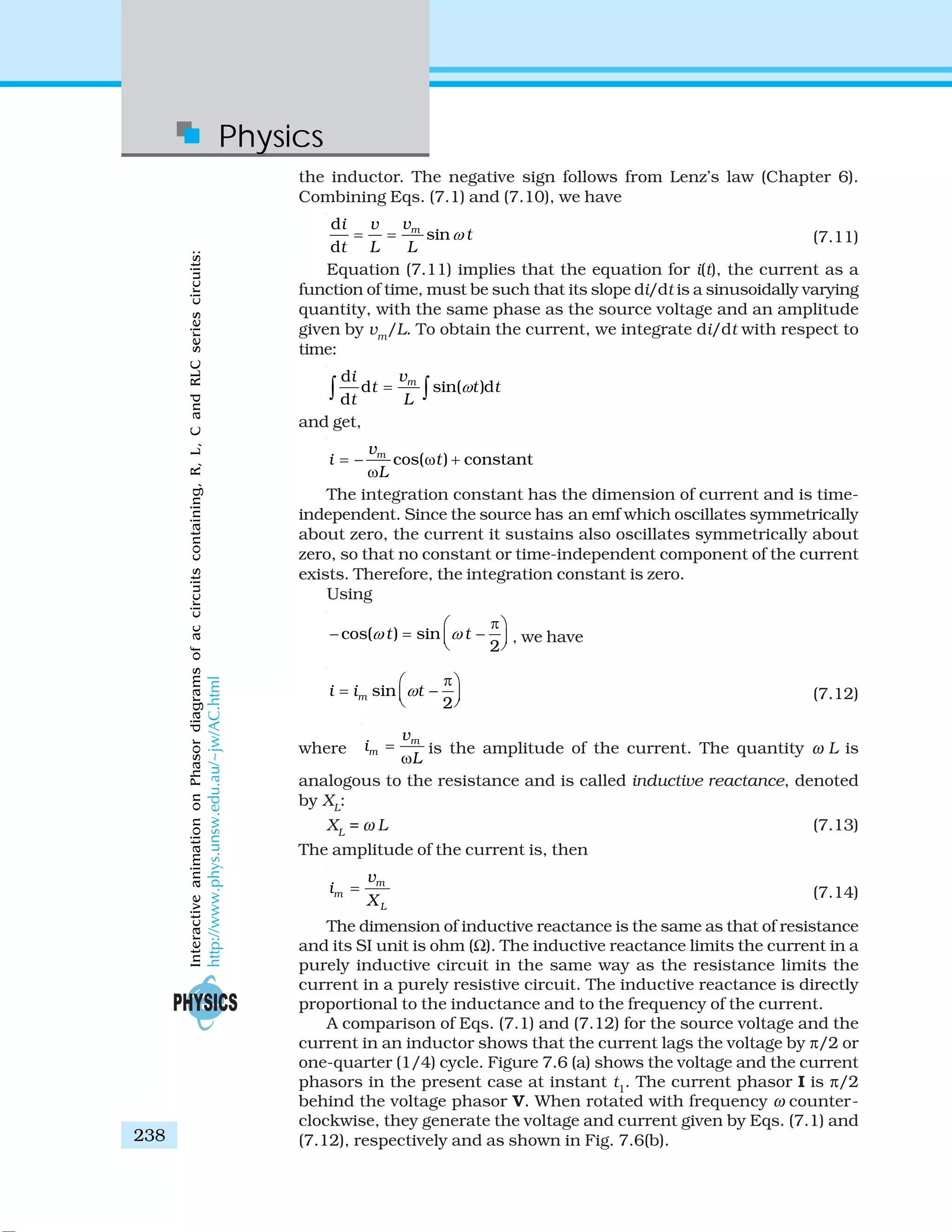
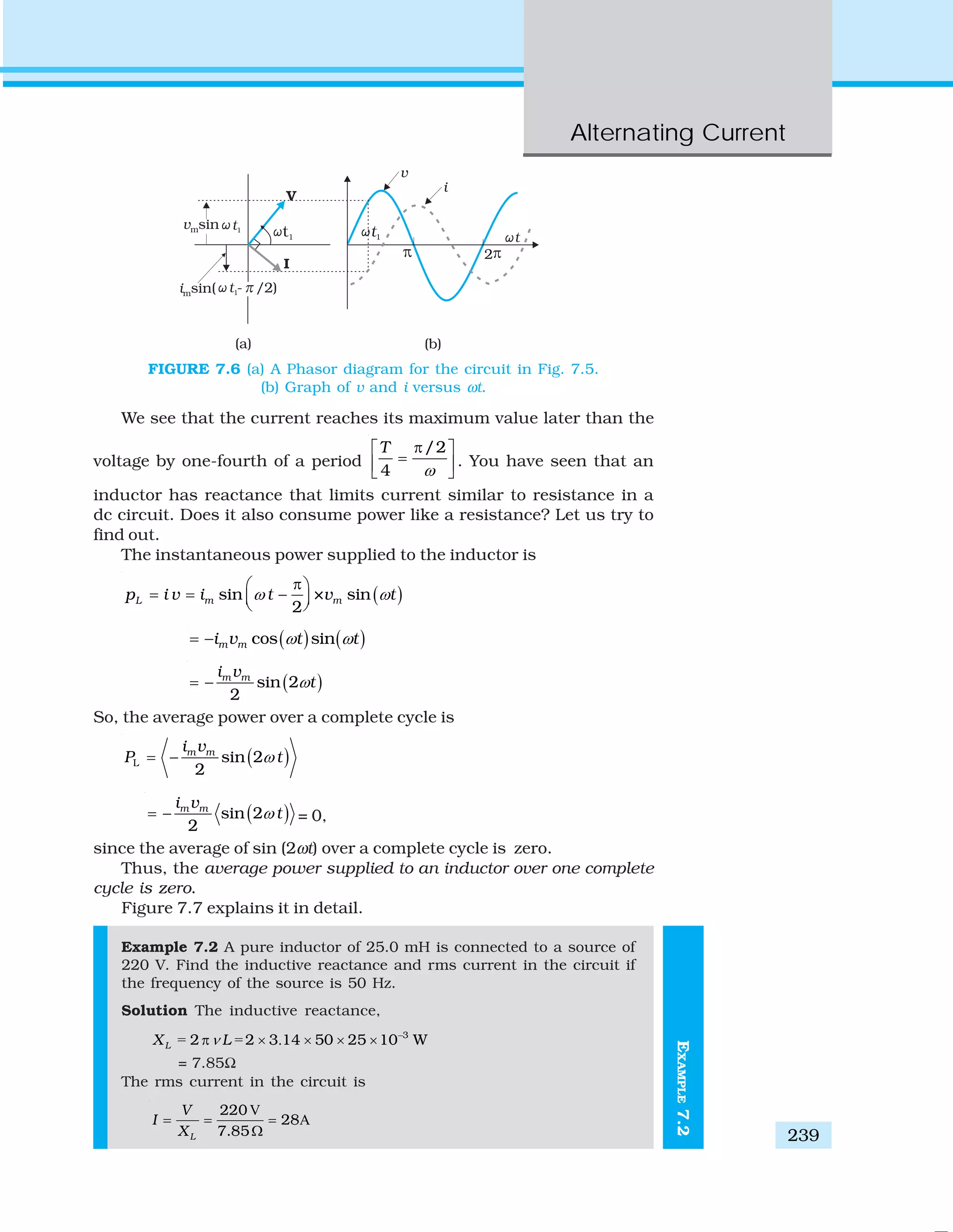
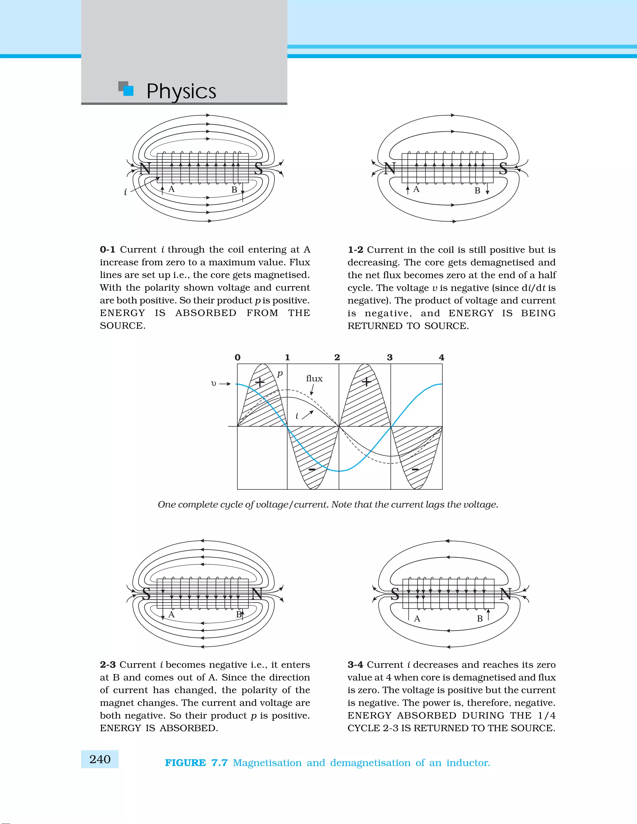
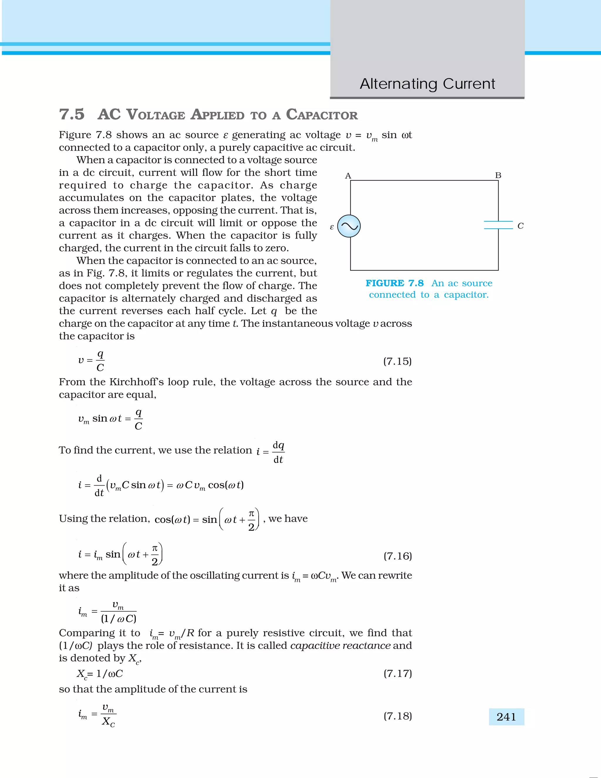
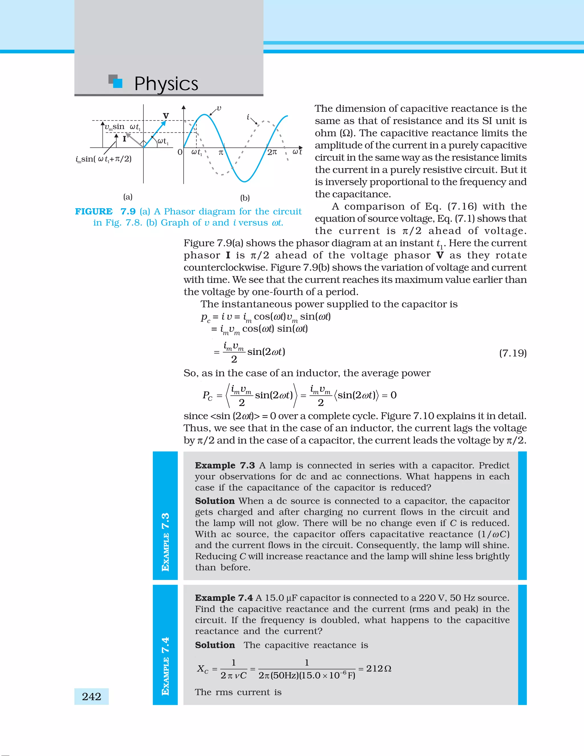
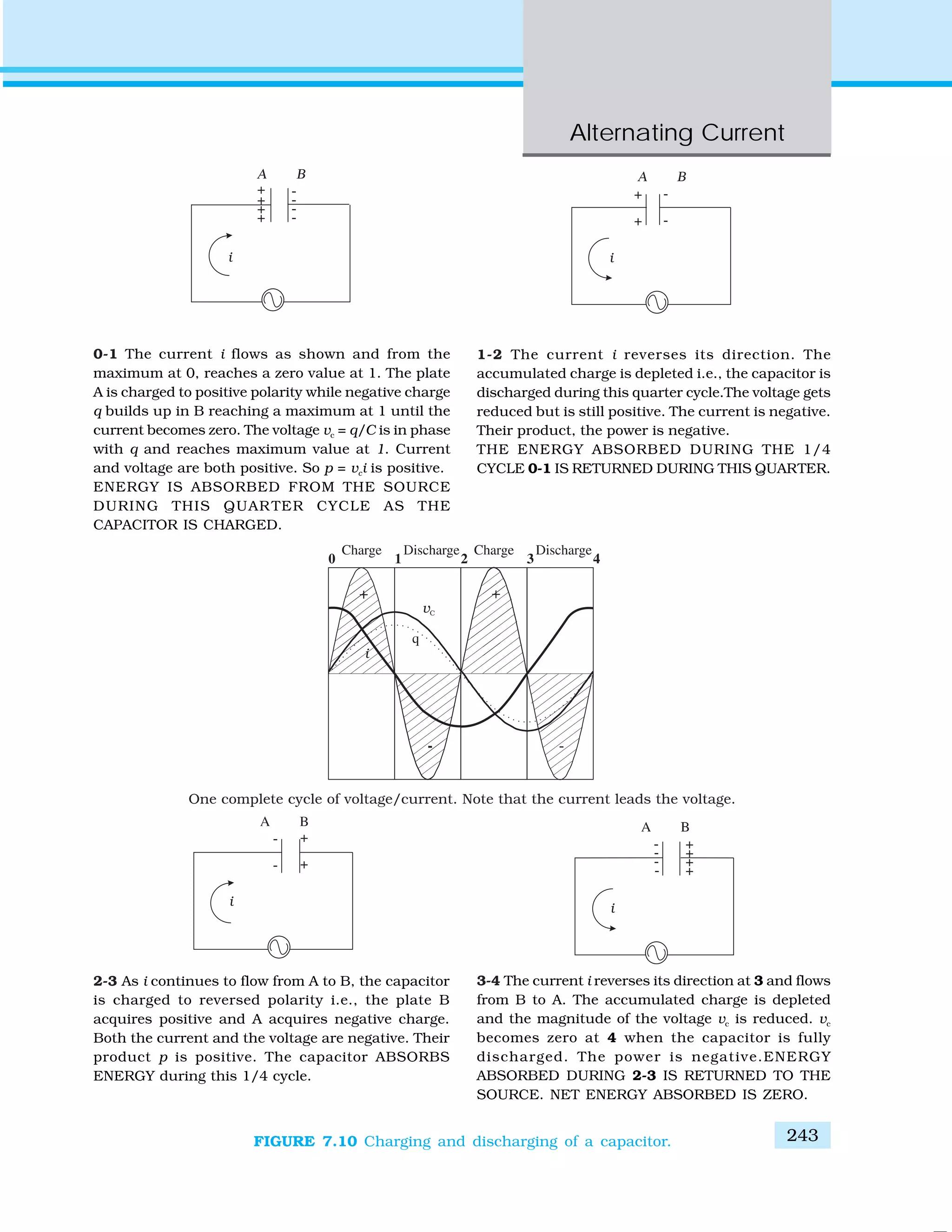
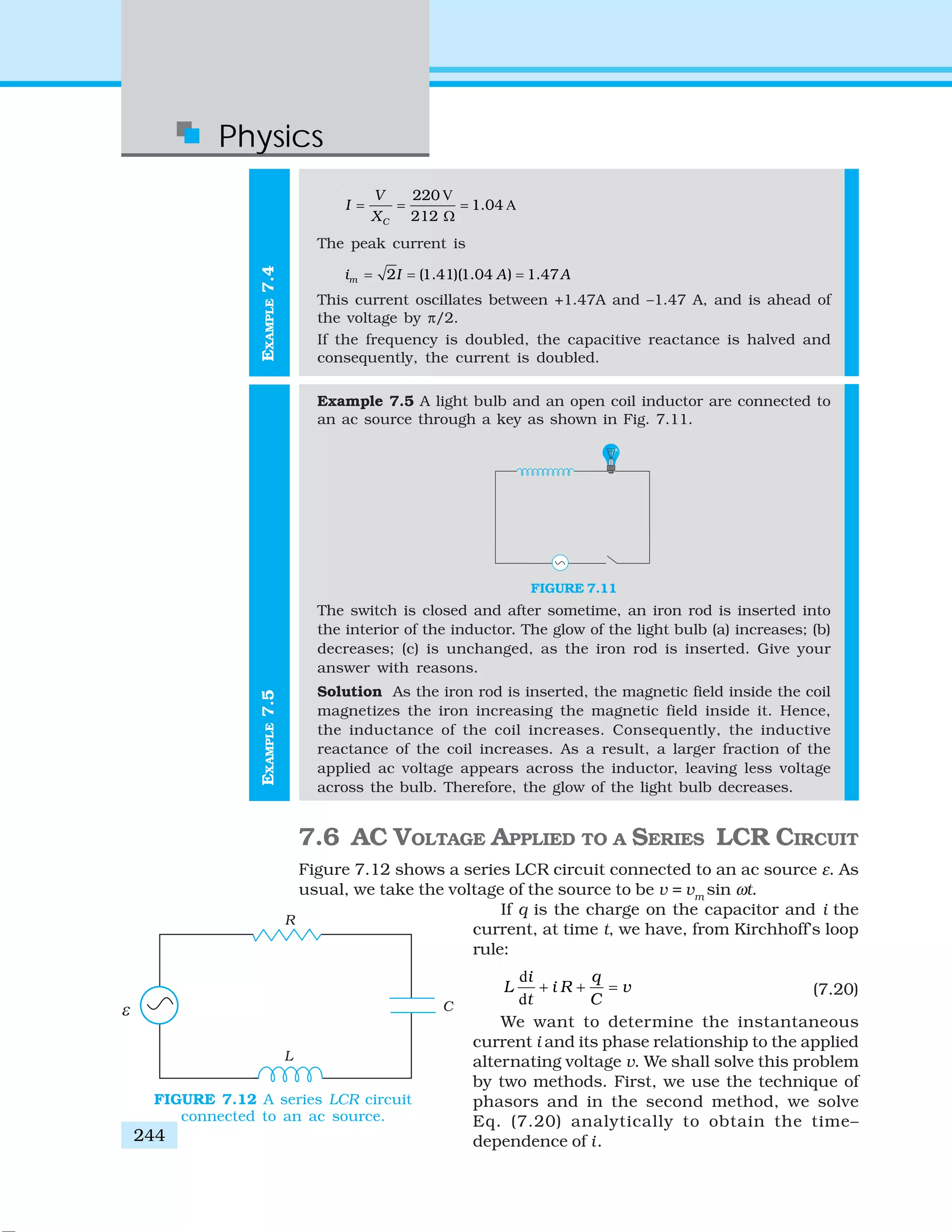
249. Alternating Current
245
7.6.1 Phasor-diagram solution
From the circuit shown in Fig. 7.12, we see that the resistor, inductor
and capacitor are in series. Therefore, the ac current in each element is
the same at any time, having the same amplitude and phase. Let it be
i = im
sin(ωt+φ) (7.21)
where φ is the phase difference between the voltage across the source and
the current in the circuit. On the basis of what we have learnt in the previous
sections, we shall construct a phasor diagram for the present case.
Let I be the phasor representing the current in the circuit as given by
Eq. (7.21). Further, let VL
, VR
, VC
, and V represent the voltage across the
inductor, resistor, capacitor and the source, respectively. From previous
section, we know that VR
is parallel to I, VC
is π/2
behind I and VL
is π/2 ahead of I. VL
, VR
, VC
and I
are shown in Fig. 7.13(a) with apppropriate phase-
relations.
The length of these phasors or the amplitude
of VR
, VC
and VL
are:
vRm
= im
R, vCm
= im
XC
, vLm
= im
XL
(7.22)
The voltage Equation (7.20) for the circuit can
be written as
vL
+ vR
+ vC
= v (7.23)
The phasor relation whose vertical component
gives the above equation is
VL
+ VR
+ VC
= V (7.24)
This relation is represented in Fig. 7.13(b). Since
VC
and VL
are always along the same line and in
opposite directions, they can be combined into a single phasor (VC
+ VL
)
which has a magnitude ⏐vCm
– vLm
⏐. Since V is represented as the
hypotenuse of a right-traingle whose sides are VR
and (VC
+ VL
), the
pythagorean theorem gives:
( )22 2
m Rm Cm Lmv v v v= + −
Substituting the values of vRm
, vCm
, and vLm
from Eq. (7.22) into the above
equation, we have
2 2 2
( ) ( )m m m C m Lv i R i X i X= + −
2 2 2
( )m C Li R X X⎡ ⎤= + −⎣ ⎦
or, 2 2
( )
m
m
C L
v
i
R X X
=
+ −
[7.25(a)]
By analogy to the resistance in a circuit, we introduce the impedance Z
in an ac circuit:
m
m
v
i
Z
= [7.25(b)]
where 2 2
( )C LZ R X X= + − (7.26)
FIGURE 7.13 (a) Relation between the
phasors VL
, VR
, VC
, and I, (b) Relation
between the phasors VL
, VR
, and (VL
+ VC
)
for the circuit in Fig. 7.11.

250. Physics
246
Since phasor I is always parallel to phasor VR
, the phase angle φ
is the angle between VR
and V and can be determined from
Fig. 7.14:
tan Cm Lm
Rm
v v
v
φ
−
=
Using Eq. (7.22), we have
tan C LX X
R
φ
−
= (7.27)
Equations (7.26) and (7.27) are graphically shown in Fig. (7.14).
This is called Impedance diagram which is a right-triangle with
Z as its hypotenuse.
Equation 7.25(a) gives the amplitude of the current and Eq. (7.27)
gives the phase angle. With these, Eq. (7.21) is completely specified.
If XC
> XL
, φ is positive and the circuit is predominantly capacitive.
Consequently, the current in the circuit leads the source voltage. If
XC
< XL
, φ is negative and the circuit is predominantly inductive.
Consequently, the current in the circuit lags the source voltage.
Figure 7.15 shows the phasor diagram and variation of v and i with ωt
for the case XC
> XL
.
Thus, we have obtained the amplitude
and phase of current for an LCR series circuit
using the technique of phasors. But this
method of analysing ac circuits suffers from
certain disadvantages. First, the phasor
diagram say nothing about the initial
condition. One can take any arbitrary value
of t (say, t1
, as done throughout this chapter)
and draw different phasors which show the
relative angle between different phasors.
The solution so obtained is called the
steady-state solution. This is not a general
solution. Additionally, we do have a
transient solution which exists even for
v = 0. The general solution is the sum of the
transient solution and the steady-state
solution. After a sufficiently long time, the effects of the transient solution
die out and the behaviour of the circuit is described by the steady-state
solution.
7.6.2 Analytical solution
The voltage equation for the circuit is
d
d
i q
L R i v
t C
+ + =
= vm
sin ωt
We know that i = dq/dt. Therefore, di/dt = d2
q/dt2
. Thus, in terms of q,
the voltage equation becomes
FIGURE 7.14 Impedance
diagram.
FIGURE 7.15 (a) Phasor diagram of V and I.
(b) Graphs of v and i versus ω t for a series LCR
circuit where XC
> XL
.

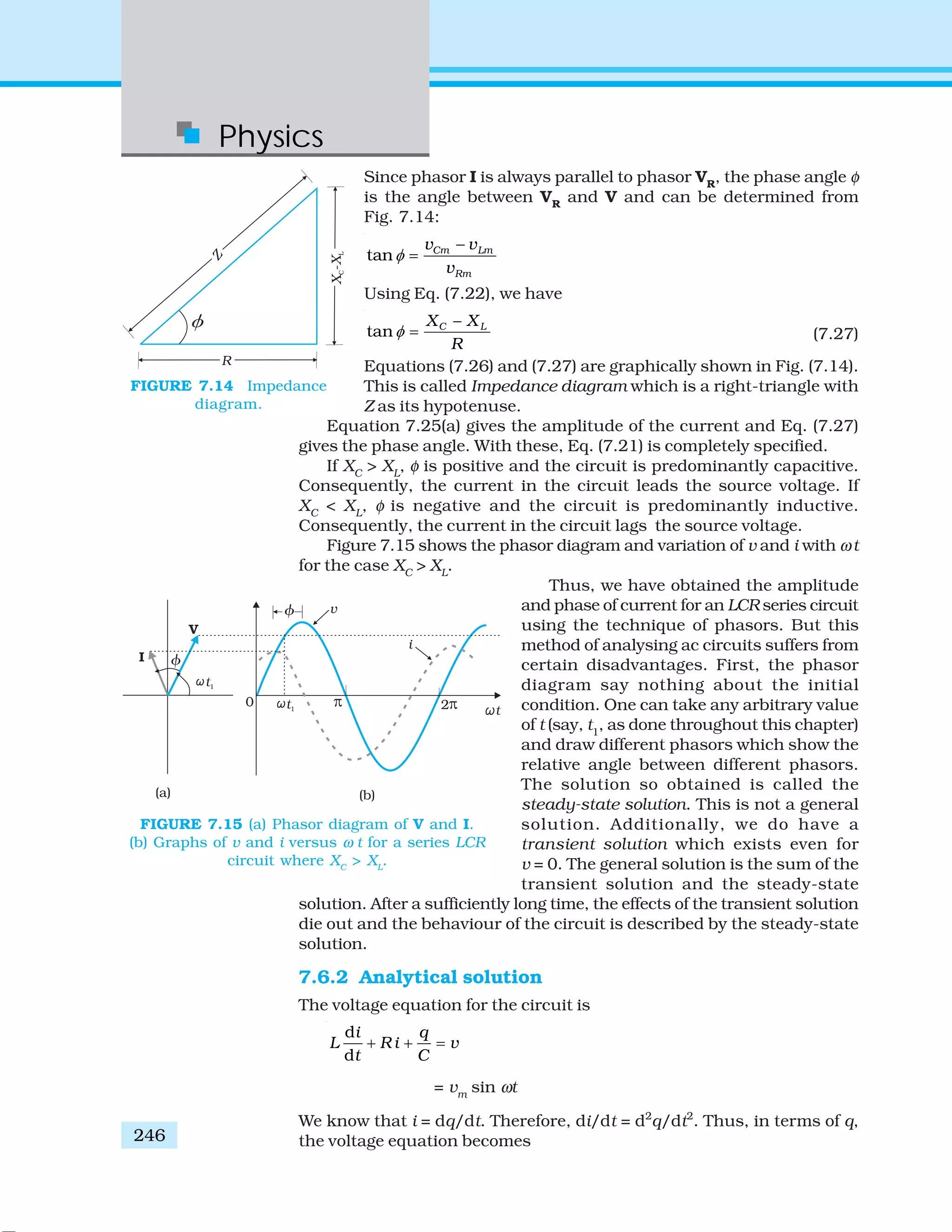
251. Alternating Current
247
2
2
d d
sin
dd
m
q q q
L R v t
t Ct
ω+ + = (7.28)
This is like the equation for a forced, damped oscillator, [see Eq. {14.37(b)}
in Class XI Physics Textbook]. Let us assume a solution
q = qm
sin (ω t + θ) [7.29(a)]
so that
d
cos( )
d
m
q
q t
t
ω ω θ= + [7.29(b)]
and
2
2
2
d
sin( )
d
m
q
q t
t
ω ω θ= − + [7.29(c)]
Substituting these values in Eq. (7.28), we get
[ ]cos( ) ( )sin( )m C Lq R t X X tω ω θ ω θ+ + − + = sinmv tω (7.30)
where we have used the relation Xc
= 1/ωC, XL
= ω L. Multiplying and
dividing Eq. (7.30) by ( )22
c LZ R X X= + − , we have
( )
cos( ) sin( )C L
m
X XR
q Z t t
Z Z
ω ω θ ω θ
−⎡ ⎤
+ + +⎢ ⎥
⎣ ⎦
sinmv tω= (7.31)
Now, let cos
R
Z
φ=
and
( )
sinC LX X
Z
φ
−
=
so that
1
tan C LX X
R
φ − −
= (7.32)
Substituting this in Eq. (7.31) and simplifying, we get:
cos( ) sinm mq Z t v tω ω θ φ ω+ − = (7.33)
Comparing the two sides of this equation, we see that
m m mv q Z i Zω= =
where
m mi q ω= [7.33(a)]
and
2
θ φ
π
− = − or
2
θ φ
π
= − + [7.33(b)]
Therefore, the current in the circuit is
d
d
cos( )m
q
i q t
t
ω ω θ= = +
= im
cos(ωt + θ)
or i = im
sin(ωt + φ) (7.34)
where 2 2
( )
m m
m
C L
v v
i
Z R X X
= =
+ −
[7.34(a)]
and
1
tan C LX X
R
φ − −
=

252. Physics
248
Thus, the analytical solution for the amplitude and phase of the current
in the circuit agrees with that obtained by the technique of phasors.
7.6.3 Resonance
An interesting characteristic of the series RLC circuit is the phenomenon
of resonance. The phenomenon of resonance is common among systems
that have a tendency to oscillate at a particular frequency. This frequency
is called the system’s natural frequency. If such a system is driven by an
energy source at a frequency that is near the natural frequency, the
amplitude of oscillation is found to be large. A familiar example of this
phenomenon is a child on a swing. The the swing has a natural frequency
for swinging back and forth like a pendulum. If the child pulls on the
rope at regular intervals and the frequency of the pulls is almost the
same as the frequency of swinging, the amplitude of the swinging will be
large (Chapter 14, Class XI).
For an RLC circuit driven with voltage of amplitude vm
and frequency
ω, we found that the current amplitude is given by
2 2
( )
m m
m
C L
v v
i
Z R X X
= =
+ −
with Xc
= 1/ωC and XL
= ωL. So if ω is varied, then at a particular frequency
ω0
, Xc
= XL
, and the impedance is minimum ( )2 2
0Z R R= + = . This
frequency is called the resonant frequency:
0
0
1
orc LX X L
C
ω
ω
= =
or 0
1
LC
ω = (7.35)
At resonant frequency, the current amplitude is maximum; im
= vm
/R.
Figure 7.16 shows the variation of im
with ω in
a RLC series circuit with L = 1.00 mH, C =
1.00 nF for two values of R: (i) R = 100 Ω
and (ii) R = 200 Ω. For the source applied vm
=
100 V. ω0
for this case is
1
LC
⎛ ⎞
⎜ ⎟⎝ ⎠ = 1.00×106
rad/s.
We see that the current amplitude is maximum
at the resonant frequency. Since im
= vm
/ R at
resonance, the current amplitude for case (i) is
twice to that for case (ii).
Resonant circuits have a variety of
applications, for example, in the tuning
mechanism of a radio or a TV set. The antenna of
a radio accepts signals from many broadcasting
stations. The signals picked up in the antenna acts as a source in the
tuning circuit of the radio, so the circuit can be driven at many frequencies.
FIGURE 7.16 Variation of im
with ω for two
cases: (i) R = 100 Ω, (ii) R = 200 Ω,
L = 1.00 mH.

253. Alternating Current
249
But to hear one particular radio station, we tune the radio. In tuning, we
vary the capacitance of a capacitor in the tuning circuit such that the
resonant frequency of the circuit becomes nearly equal to the frequency
of the radio signal received. When this happens, the amplitude of the
current with the frequency of the signal of the particular radio station in
the circuit is maximum.
It is important to note that resonance phenomenon is exhibited by a
circuit only if both L and C are present in the circuit. Only then do the
voltages across L and C cancel each other (both being out of phase)
and the current amplitude is vm
/R, the total source voltage appearing
across R. This means that we cannot have resonance in a RL or RC
circuit.
Sharpness of resonance
The amplitude of the current in the series LCR circuit is given by
2
2 1
m
m
v
i
R L
C
ω
ω
=
⎛ ⎞
+ −⎜ ⎟⎝ ⎠
and is maximum when 0 1/ .L Cω ω= = The maximum value is
max
/m mi v R= .
For values of ω other than ω0
, the amplitude of the current is less
than the maximum value. Suppose we choose a value of ω for which the
current amplitude is 1/ 2 times its maximum value. At this value, the
power dissipated by the circuit becomes half. From the curve in
Fig. (7.16), we see that there are two such values of ω, say, ω1
and ω2
, one
greater and the other smaller than ω0
and symmetrical about ω0
. We may
write
ω1
= ω0
+ Δω
ω2
= ω0
– Δω
The difference ω1
– ω2
= 2Δω is often called the bandwidth of the circuit.
The quantity (ω0
/ 2Δω) is regarded as a measure of the sharpness of
resonance. The smaller the Δω, the sharper or narrower is the resonance.
To get an expression for Δω, we note that the current amplitude im
is
( ) max
1/ 2 m
i for ω1
= ω0
+ Δω. Therefore,
1
2
2
1
1
at ,
1
m
m
v
i
R L
C
ω
ω
ω
=
⎛ ⎞
+ −⎜ ⎟
⎝ ⎠
max
2 2
m mi v
R
= =

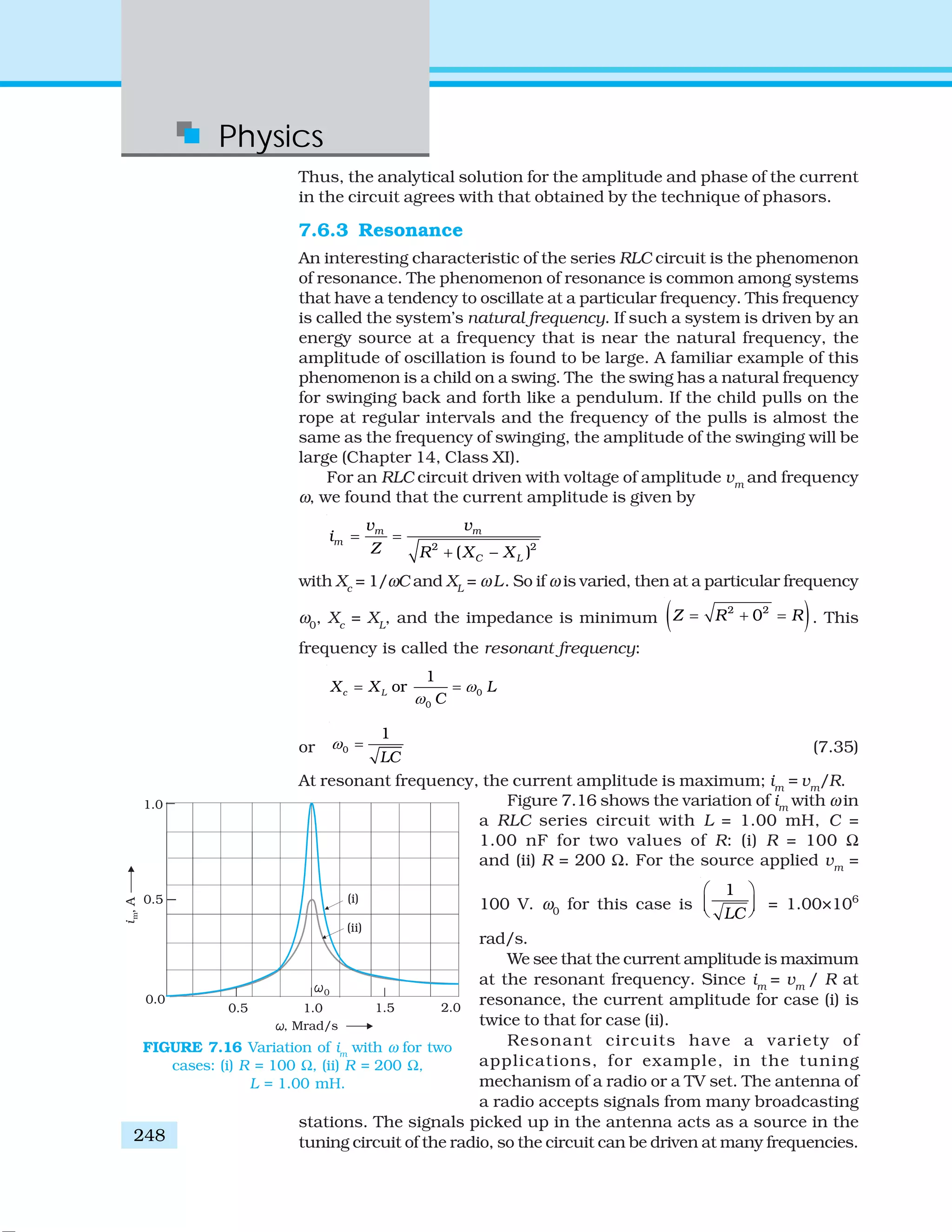
254. Physics
250
or
2
2
1
1
1
2R L R
C
ω
ω
⎛ ⎞
+ − =⎜ ⎟⎝ ⎠
or
2
2 2
1
1
1
2R L R
C
ω
ω
⎛ ⎞
+ − =⎜ ⎟⎝ ⎠
1
1
1
L R
C
ω
ω
− =
which may be written as,
0
0
1
( )
( )
L R
C
ω ω
ω ω
+ Δ − =
+ Δ
0
0
0
0
1
1
1
L R
C
ω
ω
ω ω
ω
ω
⎛ ⎞Δ
+ − =⎜ ⎟ ⎛ ⎞⎝ ⎠ Δ
+⎜ ⎟⎝ ⎠
Using 2
0
1
L C
ω = in the second term on the left hand side, we get
0
0
0
0
1
1
L
L R
ωω
ω
ω ω
ω
⎛ ⎞Δ
+ − =⎜ ⎟ ⎛ ⎞⎝ ⎠ Δ
+⎜ ⎟⎝ ⎠
We can approximate
1
0
1
ω
ω
−
⎛ ⎞Δ
+⎜ ⎟⎝ ⎠
as
0
1
ω
ω
⎛ ⎞Δ
−⎜ ⎟⎝ ⎠
since
0
ω
ω
Δ
<<1. Therefore,
0 0
0 0
1 1L L R
ω ω
ω ω
ω ω
⎛ ⎞ ⎛ ⎞Δ Δ
+ − − =⎜ ⎟ ⎜ ⎟⎝ ⎠ ⎝ ⎠
or 0
0
2
L R
ω
ω
ω
Δ
=
2
R
L
ωΔ = [7.36(a)]
The sharpness of resonance is given by,
0 0
2
L
R
ω ω
ω
=
Δ
[7.36(b)]
The ratio
0L
R
ω
is also called the quality factor, Q of the circuit.
0L
Q
R
ω
= [7.36(c)]
From Eqs. [7.36 (b)] and [7.36 (c)], we see that 0
2
Q
ω
ωΔ = . So, larger the

255. Alternating Current
251
EXAMPLE7.6
value of Q, the smaller is the value of 2Δω or the bandwidth and sharper
is the resonance. Using 2
0 1/L Cω = , Eq. [7.36(c)] can be equivalently
expressed as Q = 1/ω0
CR.
We see from Fig. 7.15, that if the resonance is less sharp, not only is
the maximum current less, the circuit is close to resonance for a larger
range Δω of frequencies and the tuning of the circuit will not be good. So,
less sharp the resonance, less is the selectivity of the circuit or vice versa.
From Eq. (7.36), we see that if quality factor is large, i.e., R is low or L is
large, the circuit is more selective.
Example 7.6 A resistor of 200 Ω and a capacitor of 15.0 μF are
connected in series to a 220 V, 50 Hz ac source. (a) Calculate the
current in the circuit; (b) Calculate the voltage (rms) across the
resistor and the capacitor. Is the algebraic sum of these voltages
more than the source voltage? If yes, resolve the paradox.
Solution
Given
F 6
200 , 15.0 15.0 10 FR C −
= Ω = μ = ×
220 V, 50HzV ν= =
(a) In order to calculate the current, we need the impedance of the
circuit. It is
2 2 2 2
(2 )CZ R X R Cπ ν −
= + = +
F2 6 2
(200 ) (2 3.14 50 10 )− −
= Ω + × × ×
2 2
(200 ) (212 )= Ω + Ω
291.5= Ω
Therefore, the current in the circuit is
V220
0.755 A
291.5
V
I
Z
= = =
Ω
(b) Since the current is the same throughout the circuit, we have
(0.755 A)(200 ) 151VRV I R= = Ω =
(0.755 A)(212.3 ) 160.3 VC CV I X= = Ω =
The algebraic sum of the two voltages, VR
and VC
is 311.3 V which is
more than the source voltage of 220 V. How to resolve this paradox?
As you have learnt in the text, the two voltages are not in the same
phase. Therefore, they cannot be added like ordinary numbers. The
two voltages are out of phase by ninety degrees. Therefore, the total
of these voltages must be obtained using the Pythagorean theorem:
2 2
R C R CV V V+ = +
= 220 V
Thus, if the phase difference between two voltages is properly taken
into account, the total voltage across the resistor and the capacitor is
equal to the voltage of the source.

256. Physics
252
EXAMPLE7.7
7.7 POWER IN AC CIRCUIT: THE POWER FACTOR
We have seen that a voltage v = vm
sinωt applied to a series RLC circuit
drives a current in the circuit given by i = im
sin(ωt + φ) where
m
m
v
i
Z
= and 1
tan C LX X
R
φ − −⎛ ⎞
= ⎜ ⎟⎝ ⎠
Therefore, the instantaneous power p supplied by the source is
( ) [ ]sin sin( )m mp v i v t i tω ω φ= = × +
[ ]cos cos(2 )
2
m mv i
tφ ω φ= − + (7.37)
The average power over a cycle is given by the average of the two terms in
R.H.S. of Eq. (7.37). It is only the second term which is time-dependent.
Its average is zero (the positive half of the cosine cancels the negative
half). Therefore,
cos
2
m mv i
P φ= cos
2 2
m mv i
φ=
cosV I φ= [7.38(a)]
This can also be written as,
2
cosP I Z φ= [7.38(b)]
So, the average power dissipated depends not only on the voltage and
current but also on the cosine of the phase angle φ between them. The
quantity cosφ is called the power factor. Let us discuss the following
cases:
Case (i) Resistive circuit: If the circuit contains only pure R, it is called
resistive. In that case φ = 0, cos φ =1.Thereis maximum power dissipation.
Case (ii) Purely inductive or capacitive circuit: If the circuit contains
only an inductor or capacitor, we know that the phase difference between
voltage and current is π/2. Therefore, cos φ = 0, and no power is dissipated
even though a current is flowing in the circuit. This current is sometimes
referred to as wattless current.
Case (iii) LCR series circuit: In an LCR series circuit, power dissipated is
given by Eq. (7.38) where φ = tan–1
(Xc
– XL
)/ R. So, φ may be non-zero in
a RL or RC or RCL circuit. Even in such cases, power is dissipated only in
the resistor.
Case (iv) Power dissipated at resonance in LCR circuit: At resonance
Xc
– XL
= 0, and φ = 0. Therefore, cosφ = 1 and P = I2
Z = I2
R. That is,
maximum power is dissipated in a circuit (through R) at resonance.
Example7.7 (a) For circuits used for transporting electric power, a
low power factor implies large power loss in transmission. Explain.
(b) Power factor can often be improved by the use of a capacitor of
appropriate capacitance in the circuit. Explain.

257. Alternating Current
253
EXAMPLE7.7
Solution (a) We know that P = I V cosφ where cosφ is the power factor.
To supply a given power at a given voltage, if cosφ is small, we have to
increase current accordingly. But this will lead to large power loss
(I2
R) in transmission.
(b)Suppose in a circuit, current I lags the voltage by an angle φ. Then
power factor cosφ =R/Z.
We can improve the power factor (tending to 1) by making Z tend to R.
Let us understand, with the help of a phasor diagram (Fig. 7.17) how
this can be achieved. Let us resolve I into two components. Ip
along
the applied voltage V and Iq
perpendicular to the applied voltage. Iq
as you have learnt in Section 7.7, is called the wattless component
since corresponding to this component of current, there is no power
loss. IP
is known as the power component because it is in phase with
the voltage and corresponds to power loss in the circuit.
It’s clear from this analysis that if we want to improve power factor,
we must completely neutralize the lagging wattless current Iq
by an
equal leading wattless current I′q
. This can be done by connecting a
capacitor of appropriate value in parallel so that Iq
and I′q
cancel
each other and P is effectively Ip
V.
Example 7.8 A sinusoidal voltage of peak value 283 V and frequency
50 Hz is applied to a series LCR circuit in which
R = 3 Ω, L = 25.48 mH, and C = 796 μF. Find (a) the impedance of the
circuit; (b) the phase difference between the voltage across the source
and the current; (c) the power dissipated in the circuit; and (d) the
power factor.
Solution
(a) To find the impedance of the circuit, we first calculate XL
and XC
.
XL
= 2 πνL
= 2 × 3.14 × 50 × 25.48 × 10–3
Ω = 8 Ω
1
2
CX
Cν
=
π
FIGURE 7.17 EXAMPLE7.8

258. Physics
254
EXAMPLE7.9
6
1
4
2 3.14 50 796 10−
= = Ω
× × × ×
Therefore,
2 2 2 2
( ) 3 (8 4)L CZ R X X= + − = + −
= 5 Ω
(b) Phase difference, φ = tan–1 C LX X
R
−
1 4 8
tan 53.1
3
− −⎛ ⎞
= = − °⎜ ⎟⎝ ⎠
Since φ is negative, the current in the circuit lags the voltage
across the source.
(c) The power dissipated in the circuit is
2
P I R=
Now, A
1 283
40
52 2
mi
I
⎛ ⎞
= = =⎜ ⎟⎝ ⎠
Therefore, A W2
(40 ) 3 4800P = × Ω =
(d) Power factor = cos cos53.1 0.6φ = ° =
Example 7.9 Suppose the frequency of the source in the previous
example can be varied. (a) What is the frequency of the source at
which resonance occurs? (b) Calculate the impedance, the current,
and the power dissipated at the resonant condition.
Solution
(a) The frequency at which the resonance occurs is
0 3 6
1 1
25.48 10 796 10LC
ω
− −
= =
× × ×
222.1rad/s=
0 221.1
Hz 35.4Hz
2 2 3.14
r
ω
ν = = =
π ×
(b) The impedance Z at resonant condition is equal to the resistance:
3Z R= = Ω
The rms current at resonance is
A
283 1
66.7
32
V V
Z R
⎛ ⎞
= = = =⎜ ⎟⎝ ⎠
The power dissipated at resonance is
2 2
(66.7) 3 13.35 kWP I R= × = × =
You can see that in the present case, power dissipated
at resonance is more than the power dissipated in Example 7.8.
EXAMPLE7.8

259. Alternating Current
255
EXAMPLE7.10
Example 7.10 At an airport, a person is made to walk through the
doorway of a metal detector, for security reasons. If she/he is carrying
anything made of metal, the metal detector emits a sound. On what
principle does this detector work?
Solution The metal detector works on the principle of resonance in
ac circuits. When you walk through a metal detector, you are,
in fact, walking through a coil of many turns. The coil is connected to
a capacitor tuned so that the circuit is in resonance. When
you walk through with metal in your pocket, the impedance of the
circuit changes – resulting in significant change in current in the
circuit. This change in current is detected and the electronic circuitry
causes a sound to be emitted as an alarm.
7.8 LC OSCILLATIONS
We know that a capacitor and an inductor can store electrical and
magnetic energy, respectively. When a capacitor (initially charged) is
connected to an inductor, the charge on the capacitor and
the current in the circuit exhibit the phenomenon of
electrical oscillations similar to oscillations in mechanical
systems (Chapter 14, Class XI).
Let a capacitor be charged qm
(at t = 0) and connected
to an inductor as shown in Fig. 7.18.
The moment the circuit is completed, the charge on
the capacitor starts decreasing, giving rise to current in
the circuit. Let q and i be the charge and current in the
circuit at time t. Since di/dt is positive, the induced emf
in L will have polarity as shown, i.e., vb
< va
. According to
Kirchhoff’s loop rule,
d
0
d
q i
L
C t
− = (7.39)
i = – (dq/dt) in the present case (as q decreases, i increases).
Therefore, Eq. (7.39) becomes:
2
2
d 1
0
d
q
q
LCt
+ = (7.40)
This equation has the form
2
2
02
d
0
d
x
x
t
ω+ = for a simple harmonic
oscillator. The charge, therefore, oscillates with a natural frequency
0
1
LC
ω = (7.41)
and varies sinusoidally with time as
( )0cosmq q tω φ= + (7.42)
where qm
is the maximum value of q and φ is a phase constant. Since
q = qm
at t = 0, we have cos φ =1 or φ = 0. Therefore, in the present case,
FIGURE 7.18 At the
instant shown, the current
is increasing so the
polarity of induced emf in
the inductor is as shown.

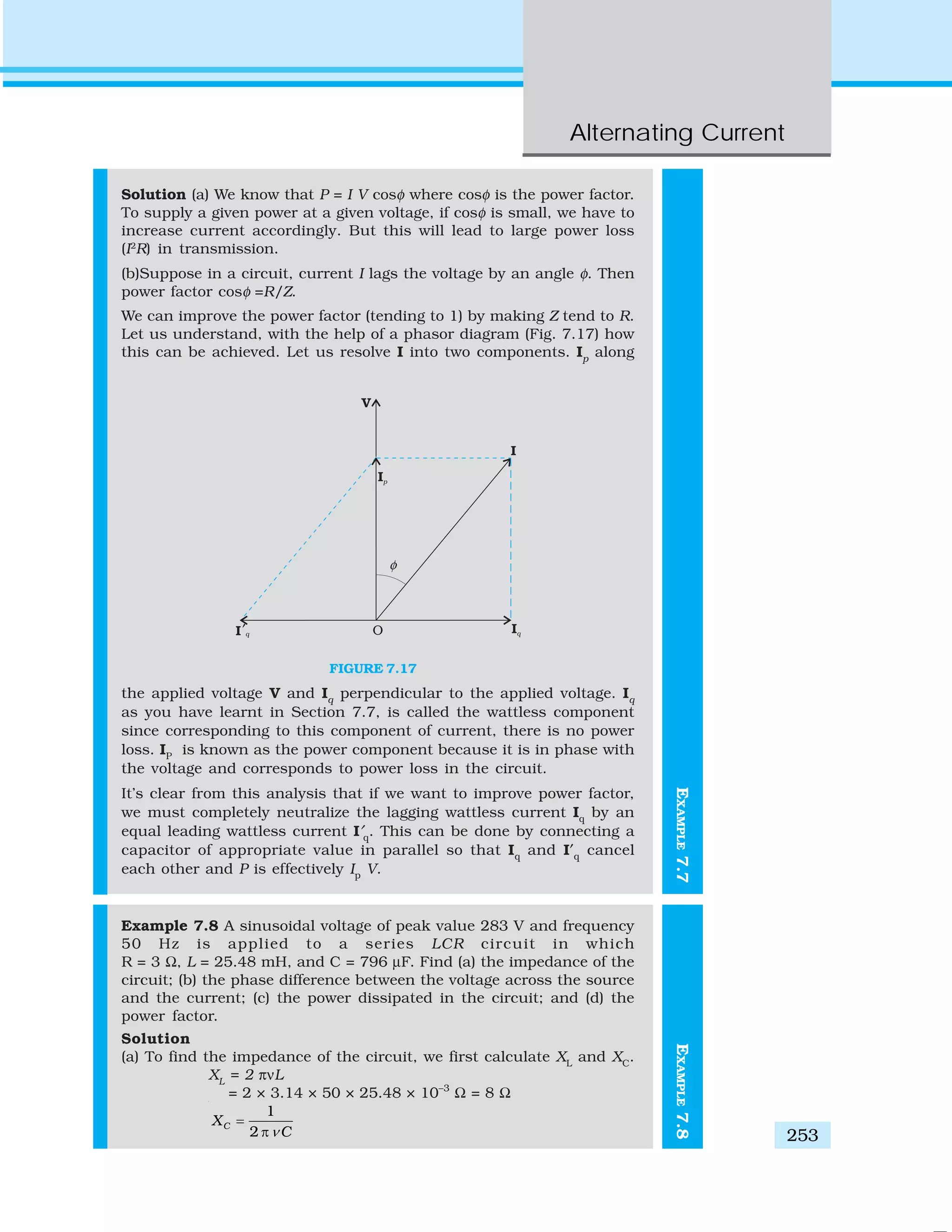
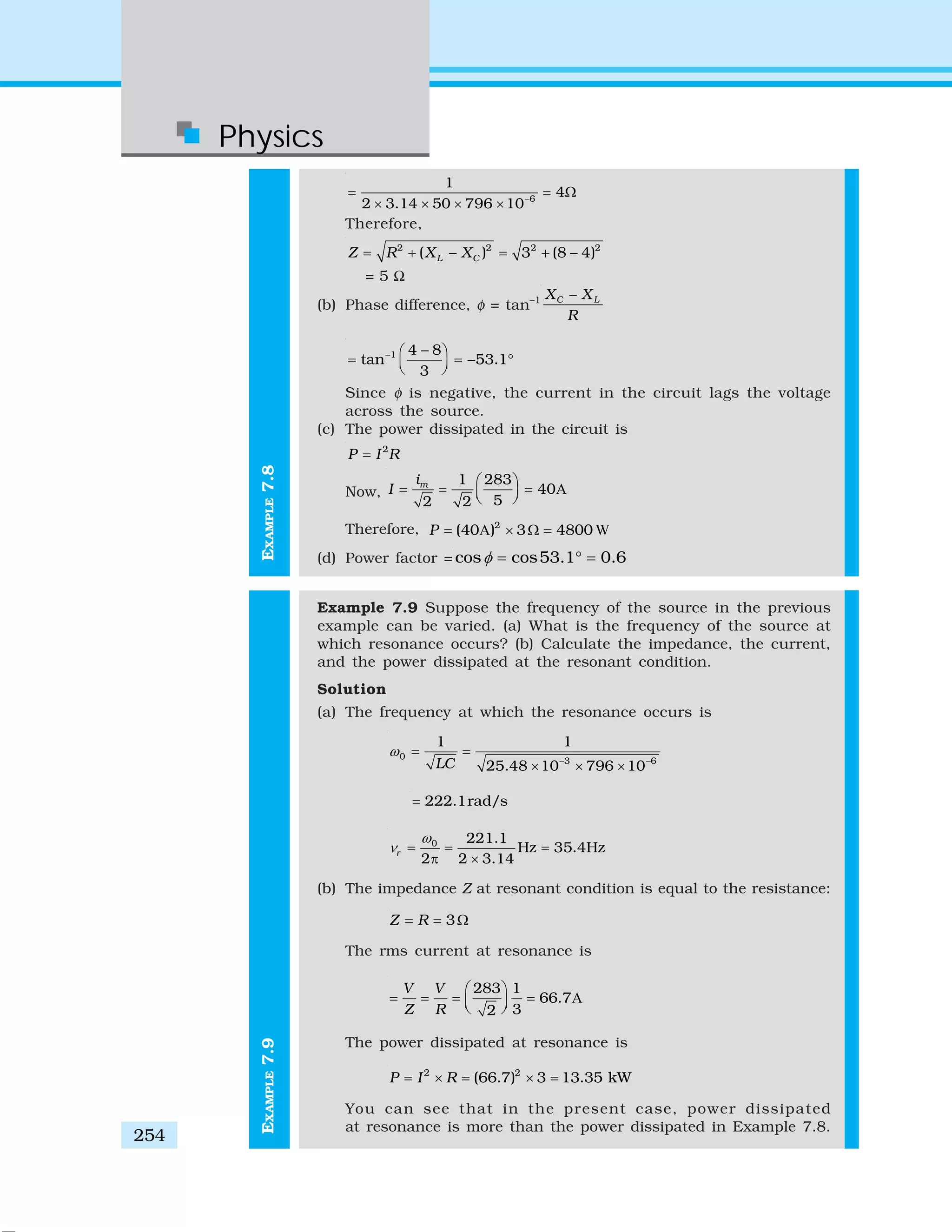
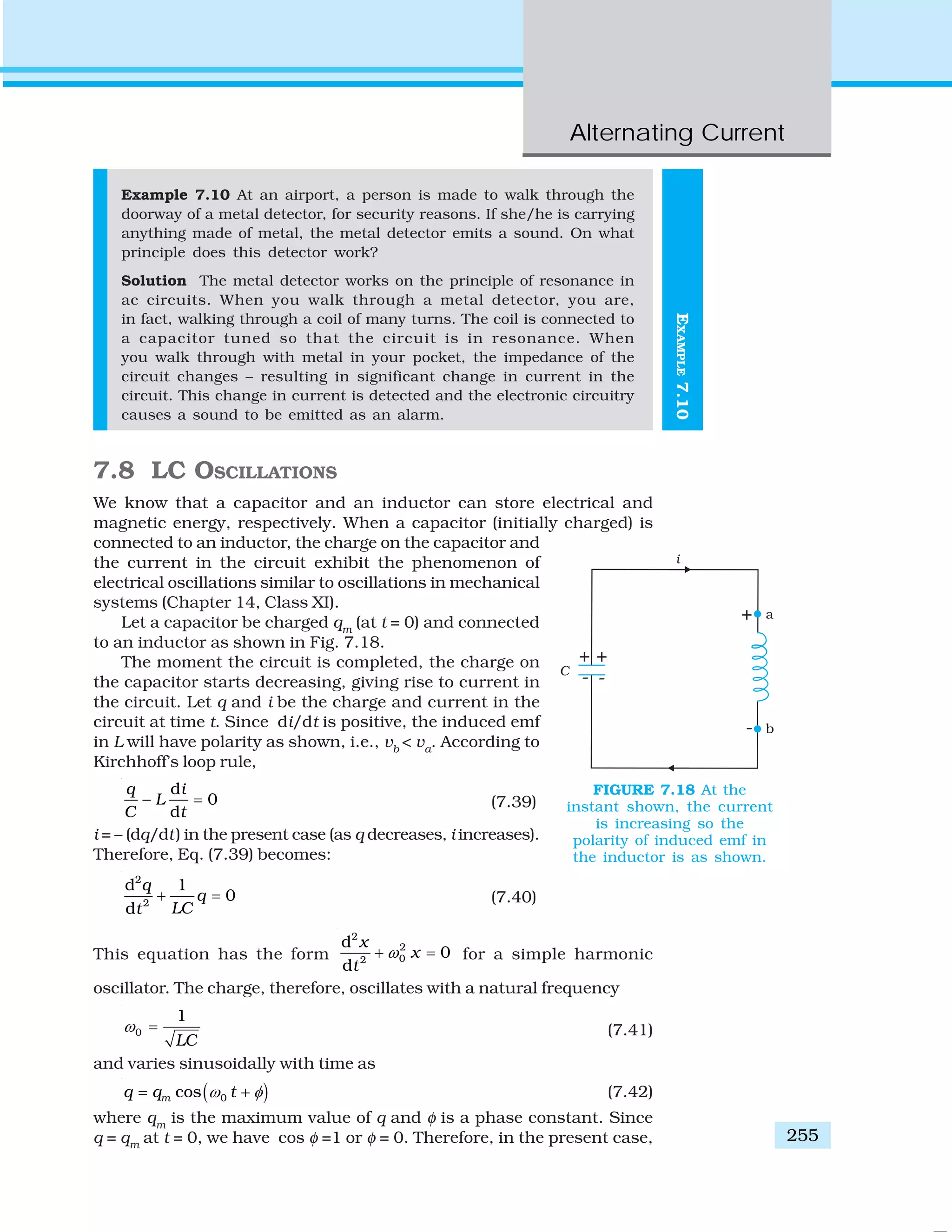
260. Physics
256
0cos( )mq q tω= (7.43)
The current
d
d
q
i
t
⎛ ⎞
= −⎜ ⎟⎝ ⎠
is given by
0sin( )mi i tω= (7.44)
where 0m mi qω=
Let us now try to visualise how this oscillation takes place in the
circuit.
Figure 7.19(a) shows a capacitor with initial charge qm
connected to
an ideal inductor. The electrical energy stored in the charged capacitor is
2
1
2
m
E
q
U
C
= . Since, there is no current in the circuit, energy in the inductor
is zero. Thus, the total energy of LC circuit is,
2
1
2
m
E
q
U U
C
= =
FIGURE 7.19 The oscillations in an LC circuit are analogous to the oscillation of a
block at the end of a spring. The figure depicts one-half of a cycle.
At t = 0, the switch is closed and the capacitor starts to discharge
[Fig. 7.19(b)]. As the current increases, it sets up a magnetic field in the
inductor and thereby, some energy gets stored in the inductor in the
form of magnetic energy: UB
= (1/2) Li2
. As the current reaches its
maximum value im
, (at t = T/4) as in Fig. 7.19(c), all the energy is stored
in the magnetic field: UB
= (1/2) Li2
m
. You can easily check that the
maximum electrical energy equals the maximum magnetic energy. The
capacitor now has no charge and hence no energy. The current now
starts charging the capacitor, as in Fig. 7.19(d). This process continues
till the capacitor is fully charged (at t = T/2) [Fig. 7.19(e)]. But it is charged
with a polarity opposite to its initial state in Fig. 7.19(a). The whole process
just described will now repeat itself till the system reverts to its original
state. Thus, the energy in the system oscillates between the capacitor
and the inductor.

261. Alternating Current
257
The LC oscillation is similar to the mechanical oscillation of a block
attached to a spring. The lower part of each figure in Fig. 7.19 depicts
the corresponding stage of a mechanical system (a block attached to a
spring). As noted earlier, for a block of a mass m oscillating with frequency
ω0
, the equation is
2
2
2 0
d
0
d
x
x
t
ω+ =
Here, 0 /k mω = , and k is the spring constant. So, x corresponds to q.
In case of a mechanical system F = ma = m (dv/dt) = m (d2
x/dt2
). For an
electrical system, ε = –L (di/dt) = –L (d2
q/dt2
). Comparing these two
equations, we see that L is analogous to mass m: L is a measure of
resistance to change in current. In case of LC circuit, 0 1/ LCω = and
for mass on a spring, 0 /k mω = . So, 1/C is analogous to k. The constant
k (=F/x) tells us the (external) force required to produce a unit
displacement whereas 1/C (=V/q) tells us the potential difference required
to store a unit charge. Table 7.1 gives the analogy between mechanical
and electrical quantities.
TABLE 7.1 ANALOGIES BETWEEN MECHANICAL AND
ELECTRICAL QUANTITIES
Mechanical system Slectrical system
Mass m Inductance L
Force constant k Reciprocal capacitance
1/C
Displacement x Charge q
Velocity v = dx/dt Current i = dq/dt
Mechanical energy Electromagnetic energy
2 21 1
2 2
E kx mv= +
2
21 1
2 2
q
U L i
C
= +
Note that the above discussion of LC oscillations is not realistic for two
reasons:
(i) Every inductor has some resistance. The effect of this resistance is to
introduce a damping effect on the charge and current in the circuit
and the oscillations finally die away.
(ii) Even if the resistance were zero, the total energy of the system would
not remain constant. It is radiated away from the system in the form
of electromagnetic waves (discussed in the next chapter). In fact, radio
and TV transmitters depend on this radiation.

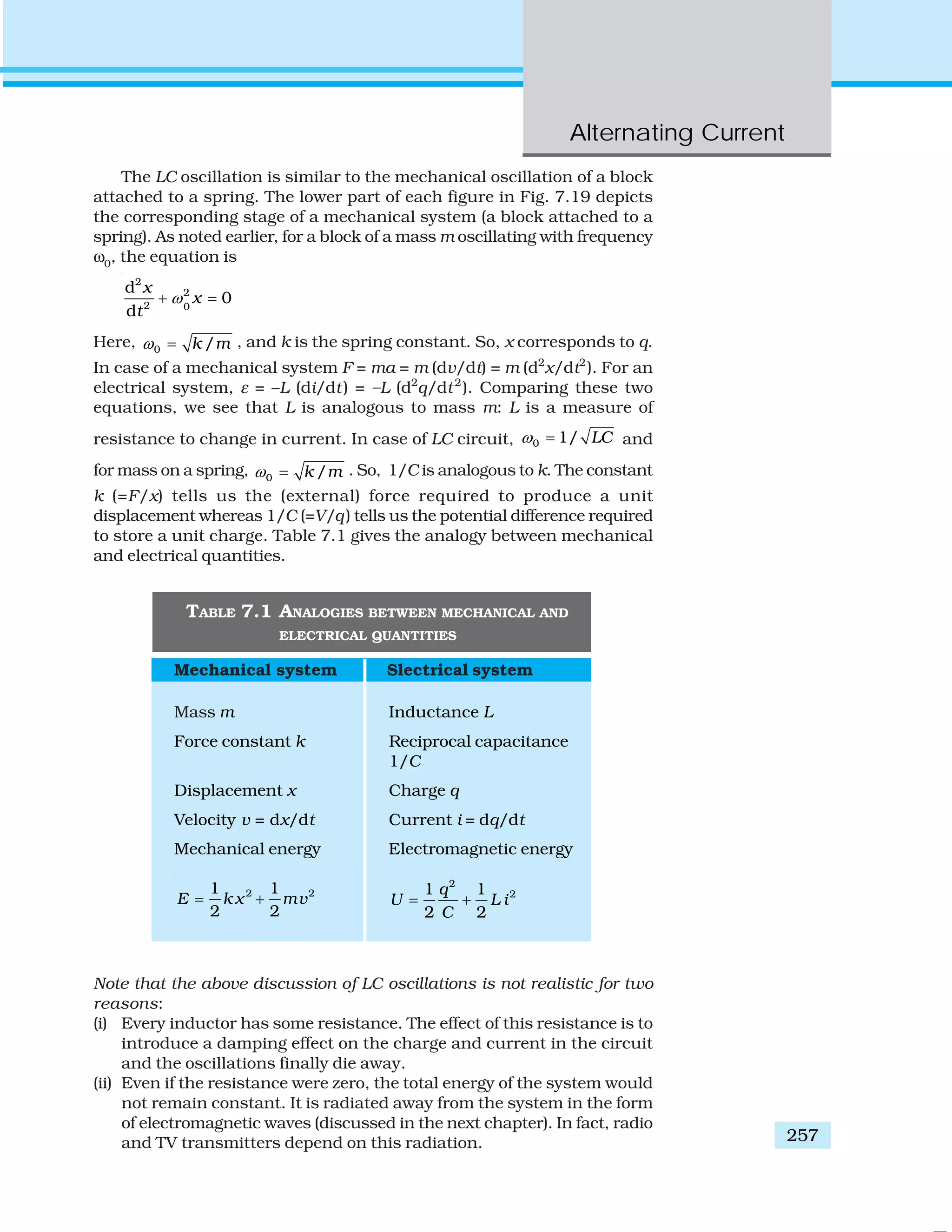
262. Physics
258
TWO DIFFERENT PHENOMENA, SAME MATHEMATICAL TREATMENT
You may like to compare the treatment of a forced damped oscillator discussed in Section
14.10 of Class XI physics textbook, with that of an LCR circuit when an ac voltage is
applied in it. We have already remarked that Eq. [14.37(b)] of Class XI Textbook is exactly
similar to Eq. (7.28) here, although they use different symbols and parameters. Let us
therefore list the equivalence between different quantities in the two situations:
Forced oscillations Driven LCR circuit
cos d
2d x dxm b kx F
2 dtdt
tω+ + =
2
2
d d
sin
dd
m
q q q
L R v t
t Ct
ω+ + =
Displacement, x Charge on capacitor, q
Time, t Time, t
Mass, m Self inductance, L
Damping constant, b Resistance, R
Spring constant, k Inverse capacitance, 1/C
Driving frequency, ωd
Driving frequency, ω
Natural frequency of oscillations, ω Natural frequency of LCR circuit, ω0
Amplitude of forced oscillations, A Maximum charge stored, qm
Amplitude of driving force, F0
Amplitude of applied voltage, vm
You must note that since x corresponds to q, the amplitude A (maximum displacement)
will correspond to the maximum charge stored, qm
. Equation [14.39 (a)] of Class XI gives
the amplitude of oscillations in terms of other parameters, which we reproduce here for
convenience:
{ }
0
1/22 2 2 2 2 2
( )d d
F
A
m bω ω ω
=
− +
Replace each parameter in the above equation by the corresponding electrical
quantity, and see what happens. Eliminate L, C, ω , and ω
0
, using XL
= ωL, XC
= 1/ωC, and
ω0
2
= 1/LC. When you use Eqs. (7.33) and (7.34), you will see that there is a
perfect match.
You will come across numerous such situations in physics where diverse physical
phenomena are represented by the same mathematical equation. If you have dealt with
one of them, and you come across another situation, you may simply replace the
corresponding quantities and interpret the result in the new context. We suggest that
you may try to find more such parallel situations from different areas of physics. One
must, of course, be aware of the differences too.

263. Alternating Current
259
EXAMPLE7.11
Example 7.11 Show that in the free oscillations of an LC circuit, the
sum of energies stored in the capacitor and the inductor is constant
in time.
Solution Let q0
be the initial charge on a capacitor. Let the charged
capacitor be connected to an inductor of inductance L. As you have
studied in Section 7.8, this LC circuit will sustain an oscillation with
frquency
ω
1
2
LC
π ν
⎛ ⎞
= =⎜ ⎟⎝ ⎠
At an instant t, charge q on the capacitor and the current i are given
by:
q (t) = q0
cos ωt
i (t) = – q0
ω sin ωt
Energy stored in the capacitor at time t is
22
2 201 1
( )
2 2 2
E
qq
U C V cos t
C C
ω= = =
Energy stored in the inductor at time t is
21
2
MU L i=
2 2 2
0
1
sin ( )
2
L q tω ω=
( )
2
2 20
sin ( ) 1/
2
q
t LC
C
ω ω= =∵
Sum of energies
2
2 20
cos sin
2
E M
q
U U t t
C
ω ω⎡ ⎤+ = +⎣ ⎦
2
0
2
q
C
=
This sum is constant in time as qo
and C, both are time-independent.
Note that it is equal to the initial energy of the capacitor. Why it is
so? Think!
7.9 TRANSFORMERS
For many purposes, it is necessary to change (or transform) an alternating
voltage from one to another of greater or smaller value. This is done with
a device called transformer using the principle of mutual induction.
A transformer consists of two sets of coils, insulated from each other.
They are wound on a soft-iron core, either one on top of the other as in
Fig. 7.20(a) or on separate limbs of the core as in Fig. 7.20(b). One of the
coils called the primary coil has Np
turns. The other coil is called the
secondary coil; it has Ns
turns. Often the primary coil is the input coil
and the secondary coil is the output coil of the transformer.

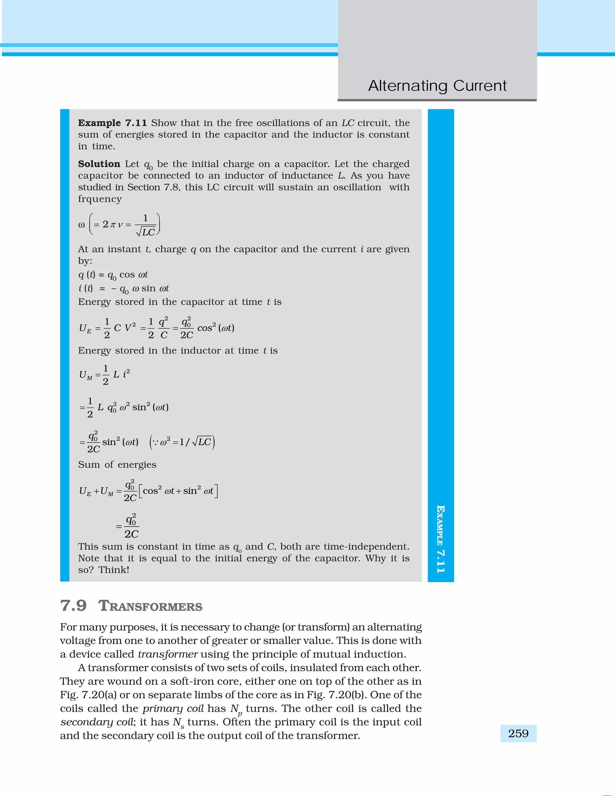
264. Physics
260
When an alternating voltage is applied to the primary, the resulting
current produces an alternating magnetic flux which links the secondary
and induces an emf in it. The value of this emf depends on the number of
turns in the secondary. We consider an ideal transformer in which the
primary has negligible resistance and all the flux in the core links both
primary and secondary windings. Let φ be the flux in each turn in the
core at time t due to current in the primary when a voltage vp
is applied
to it.
Then the induced emf or voltage εs
, in the secondary with Ns
turns is
d
d
s sN
t
φ
ε = − (7.45)
The alternating flux φ also induces an emf, called back emf in the
primary. This is
d
d
p pN
t
φ
ε = − (7.46)
But εp
= vp
. If this were not so, the primary current would be infinite
since the primary has zero resistance(as assumed). If the secondary is
an open circuit or the current taken from it is small, then to a good
approximation
εs
= vs
where vs
is the voltage across the secondary. Therefore, Eqs. (7.45) and
(7.46) can be written as
s s
d
v N
d t
φ
= − [7.45(a)]
p p
d
v N
d t
φ
= − [7.46(a)]
From Eqs. [7.45 (a)] and [7.45 (a)], we have
s s
p p
v N
v N
= (7.47)
FIGURE 7.20 Two arrangements for winding of primary and secondary coil in a transformer:
(a) two coils on top of each other, (b) two coils on separate limbs of the core.

265. Alternating Current
261
Note that the above relation has been obtained using three
assumptions: (i) the primary resistance and current are small; (ii) the
same flux links both the primary and the secondary as very little flux
escapes from the core, and (iii) the secondary current is small.
If the transformer is assumed to be 100% efficient (no energy losses),
the power input is equal to the power output, and since p = i v,
ip
vp
= is
vs
(7.48)
Although some energy is always lost, this is a good approximation,
since a well designed transformer may have an efficiency of more than
95%. Combining Eqs. (7.47) and (7.48), we have
p s s
s p p
i v N
i v N
= = (7.49)
Since i and v both oscillate with the same frequency as the ac source,
Eq. (7.49) also gives the ratio of the amplitudes or rms values of
corresponding quantities.
Now, we can see how a transformer affects the voltage and current.
We have:
s
s p
p
N
V V
N
⎛ ⎞
= ⎜ ⎟
⎝ ⎠
and
p
s p
s
N
I I
N
⎛ ⎞
= ⎜ ⎟⎝ ⎠
(7.50)
That is, if the secondary coil has a greater number of turns than the
primary (Ns
> Np
), the voltage is stepped up(Vs
> Vp
). This type of
arrangement is called a step-up transformer. However, in this arrangement,
there is less current in the secondary than in the primary (Np
/Ns
< 1 and Is
< Ip
). For example, if the primary coil of a transformer has 100 turns and
the secondary has 200 turns, Ns
/Np
= 2 and Np
/Ns
=1/2. Thus, a 220V
input at 10A will step-up to 440 V output at 5.0 A.
If the secondary coil has less turns than the primary(Ns
< Np
), we have
a step-down transformer. In this case, Vs
< Vp
and Is
> Ip
. That is, the
voltage is stepped down, or reduced, and the current is increased.
The equations obtained above apply to ideal transformers (without
any energy losses). But in actual transformers, small energy losses do
occur due to the following reasons:
(i) Flux Leakage: There is always some flux leakage; that is, not all of
the flux due to primary passes through the secondary due to poor
design of the core or the air gaps in the core. It can be reduced by
winding the primary and secondary coils one over the other.
(ii) Resistance of the windings: The wire used for the windings has some
resistance and so, energy is lost due to heat produced in the wire
(I 2
R). In high current, low voltage windings, these are minimised by
using thick wire.
(iii) Eddy currents: The alternating magnetic flux induces eddy currents
in the iron core and causes heating. The effect is reduced by having a
laminated core.
(iv) Hysteresis: The magnetisation of the core is repeatedly reversed by
the alternating magnetic field. The resulting expenditure of energy in
the core appears as heat and is kept to a minimum by using a magnetic
material which has a low hysteresis loss.

266. Physics
262
The large scale transmission and distribution of electrical energy over
long distances is done with the use of transformers. The voltage output
of the generator is stepped-up (so that current is reduced and
consequently, the I2
R loss is cut down). It is then transmitted over long
distances to an area sub-station near the consumers. There the voltage
is stepped down. It is further stepped down at distributing sub-stations
and utility poles before a power supply of 240 V reaches our homes.
SUMMARY
1. An alternating voltage sinm
v v t= ω applied to a resistor R drives a
current i = im
sinωt in the resistor,
m
m
v
i
R
= . The current is in phase with
the applied voltage.
2. For an alternating current i = im
sinωt passing through a resistor R, the
average power loss P (averaged over a cycle) due to joule heating is
( 1/2 )i2
m
R. To express it in the same form as the dc power (P = I 2
R), a
special value of current is used. It is called root mean square (rms)
current and is donoted by I:
0.707
2
m
m
i
I i= =
Similarly, the rms voltage is defined by
0.707
2
m
m
v
V v= =
We have P = IV = I2
R
3. An ac voltage v = vm
sinωt applied to a pure inductor L, drives a current
in the inductor i = im
sin (ωt – π/2), where im
= vm
/XL
. XL
= ωL is called
inductive reactance. The current in the inductor lags the voltage by
π/2. The average power supplied to an inductor over one complete cycle
is zero.
4. An ac voltage v = vm
sinωt applied to a capacitor drives a current in the
capacitor: i = im
sin (ωt + π/2). Here,
1
,m
m C
C
v
i X
X Cω
= = is called capacitive reactance.
The current through the capacitor is π/2 ahead of the applied voltage.
As in the case of inductor, the average power supplied to a capacitor
over one complete cycle is zero.
5. For a series RLC circuit driven by voltage v = vm
sinωt, the current is
given by i = im
sin (ωt + φ)
where
( )22
m
m
C L
v
i
R X X
=
+ −
and 1
tan C LX X
R
φ − −
=
( )22
C LZ R X X= + − is called the impedance of the circuit.

267. Alternating Current
263
The average power loss over a complete cycle is given by
P = V I cosφ
The term cosφ is called the power factor.
6. In a purely inductive or capacitive circuit, cosφ = 0 and no power is
dissipated even though a current is flowing in the circuit. In such cases,
current is referred to as a wattless current.
7. The phase relationship between current and voltage in an ac circuit
can be shown conveniently by representing voltage and current by
rotating vectors called phasors. A phasor is a vector which rotates
about the origin with angular speed ω. The magnitude of a phasor
represents the amplitude or peak value of the quantity (voltage or
current) represented by the phasor.
The analysis of an ac circuit is facilitated by the use of a phasor
diagram.
8. An interesting characteristic of a series RLC circuit is the
phenomenon of resonance. The circuit exhibits resonance, i.e.,
the amplitude of the current is maximum at the resonant
frequency, 0
1
LC
ω = . The quality factor Q defined by
0L
Q
R
ω
=
0
1
CRω
= is an indicator of the sharpness of the resonance,
the higher value of Q indicating sharper peak in the current.
9. A circuit containing an inductor L and a capacitor C (initially
charged) with no ac source and no resistors exhibits free
oscillations. The charge q of the capacitor satisfies the equation
of simple harmonic motion:
2
2
d 1
0
q
q
LCdt
+ =
and therefore, the frequency ω of free oscillation is 0
1
LC
ω = . The
energy in the system oscillates between the capacitor and the
inductor but their sum or the total energy is constant in time.
10. A transformer consists of an iron core on which are bound a
primary coil of Np
turns and a secondary coil of Ns
turns. If the
primary coil is connected to an ac source, the primary and
secondary voltages are related by
s
s p
p
N
V V
N
⎛ ⎞
= ⎜ ⎟
⎝ ⎠
and the currents are related by
p
ps
s
N
I I
N
⎛ ⎞
= ⎜ ⎟⎝ ⎠
If the secondary coil has a greater number of turns than the primary, the
voltage is stepped-up (Vs
> Vp
). This type of arrangement is called a step-
up transformer. If the secondary coil has turns less than the primary, we
have a step-down transformer.

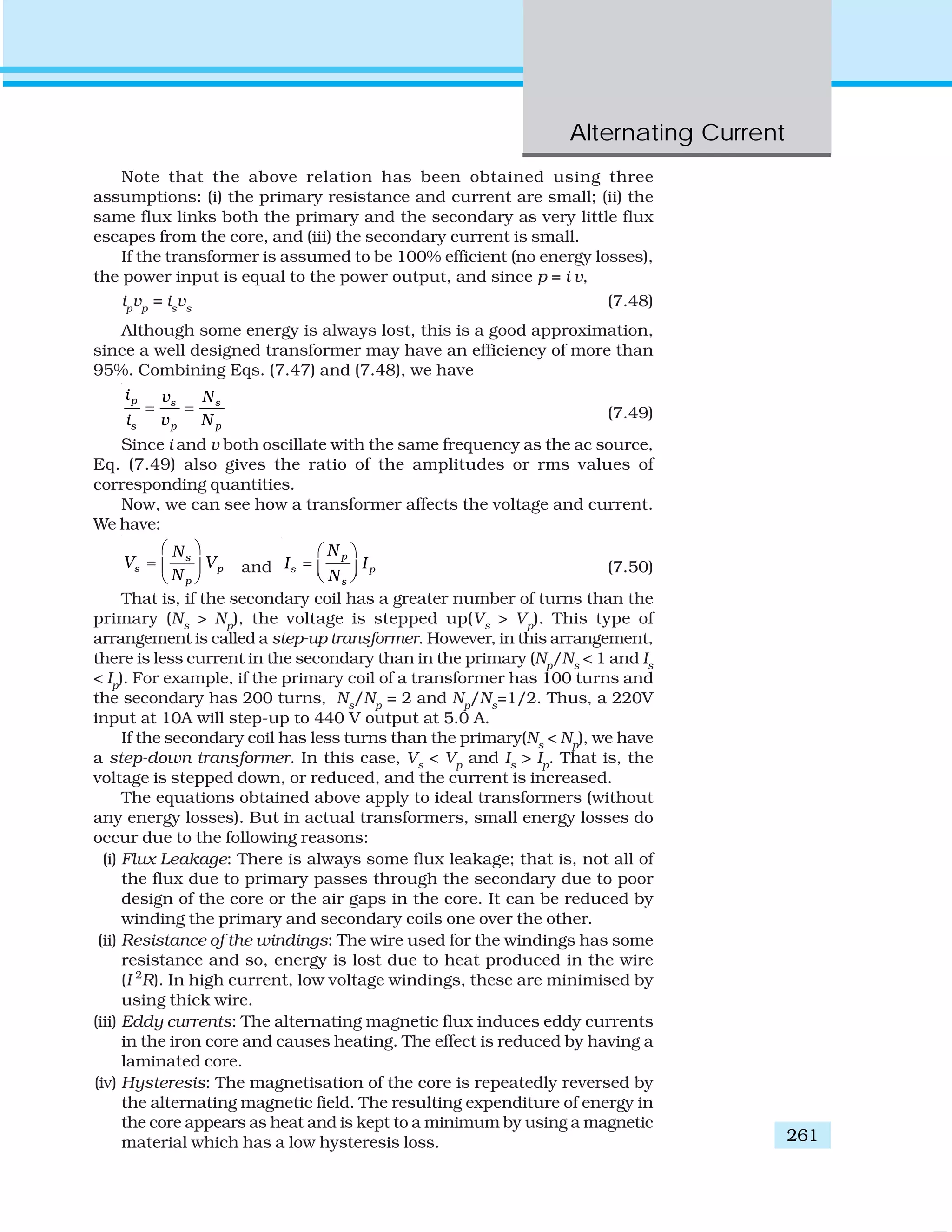
268. Physics
264
Physical quantity Symbol Dimensions Unit Remarks
rms voltage V [M L2
T–3
A–1
] V V =
2
mv
, vm
is the
amplitude of the ac voltage.
rms current I [ A] A I =
2
mi
, im
is the amplitude of
the ac current.
Reactance:
Inductive XL
[M L
2
T
–3
A
–2
] Ω XL
= ω L
Capacitive XC
[M L
2
T
–3
A
–2
] Ω XC
= 1/ω C
Impedance Z [M L2
T–3
A–2
] Ω Depends on elements
present in the circuit.
Resonant ωr
or ω0
[T
–1
] Hz ω0
LC
1
= for a
frequency
series RLC circuit
Quality factor Q Dimensionless 0
0
1L
Q
R C R
ω
ω
= = for a series
RLC circuit.
Power factor Dimensionless = cosφ, φ is the phase
difference between voltage
applied and current in
the circuit.
POINTS TO PONDER
1. When a value is given for ac voltage or current, it is ordinarily the rms
value. The voltage across the terminals of an outlet in your room is
normally 240 V. This refers to the rms value of the voltage. The amplitude
of this voltage is
V2 2(240) 340mv V= = =
2. The power rating of an element used in ac circuits refers to its average
power rating.
3. The power consumed in an circuit is never negative.
4. Both alternating current and direct current are measured in amperes.
But how is the ampere defined for an alternating current? It cannot be
derived from the mutual attraction of two parallel wires carrying ac
currents, as the dc ampere is derived. An ac current changes direction

269. Alternating Current
265
with the source frequency and the attractive force would average to
zero. Thus, the ac ampere must be defined in terms of some property
that is independent of the direction of the current. Joule heating
is such a property, and there is one ampere of rms value of
alternating current in a circuit if the current produces the same
average heating effect as one ampere of dc current would produce
under the same conditions.
5. In an ac circuit, while adding voltages across different elements, one
should take care of their phases properly. For example, if VR
and VC
are voltages across R and C, respectively in an RC circuit, then the
total voltage across RC combination is 2 2
RC R CV V V= + and not
VR
+ VC
since VC
is π/2 out of phase of VR
.
6. Though in a phasor diagram, voltage and current are represented by
vectors, these quantities are not really vectors themselves. They are
scalar quantities. It so happens that the amplitudes and phases of
harmonically varying scalars combine mathematically in the same
way as do the projections of rotating vectors of corresponding
magnitudes and directions. The ‘rotating vectors’ that represent
harmonically varying scalar quantities are introduced only to provide
us with a simple way of adding these quantities using a rule that
we already know as the law of vector addition.
7. There are no power losses associated with pure capacitances and pure
inductances in an ac circuit. The only element that dissipates energy
in an ac circuit is the resistive element.
8. In a RLC circuit, resonance phenomenon occur when XL
= XC
or
0
1
LC
ω = . For resonance to occur, the presence of both L and C
elements in the circuit is a must. With only one of these (L or C )
elements, there is no possibility of voltage cancellation and hence,
no resonance is possible.
9. The power factor in a RLC circuit is a measure of how close the
circuit is to expending the maximum power.
10. In generators and motors, the roles of input and output are
reversed. In a motor, electric energy is the input and mechanical
energy is the output. In a generator, mechanical energy is the
input and electric energy is the output. Both devices simply
transform energy from one form to another.
11. A transformer (step-up) changes a low-voltage into a high-voltage.
This does not violate the law of conservation of energy. The
current is reduced by the same proportion.
12. The choice of whether the description of an oscillatory motion is
by means of sines or cosines or by their linear combinations is
unimportant, since changing the zero-time position transforms
the one to the other.

270. Physics
266
EXERCISES
7.1 A 100 Ω resistor is connected to a 220 V, 50 Hz ac supply.
(a) What is the rms value of current in the circuit?
(b) What is the net power consumed over a full cycle?
7.2 (a) The peak voltage of an ac supply is 300 V. What is the rms voltage?
(b) The rms value of current in an ac circuit is 10 A. What is the
peak current?
7.3 A 44 mH inductor is connected to 220 V, 50 Hz ac supply. Determine
the rms value of the current in the circuit.
7.4 A 60 μF capacitor is connected to a 110 V, 60 Hz ac supply. Determine
the rms value of the current in the circuit.
7.5 In Exercises 7.3 and 7.4, what is the net power absorbed by each
circuit over a complete cycle. Explain your answer.
7.6 Obtain the resonant frequency ωr
of a series LCR circuit with
L = 2.0H, C = 32 μF and R = 10 Ω. What is the Q-value of this circuit?
7.7 A charged 30 μF capacitor is connected to a 27 mH inductor. What is
the angular frequency of free oscillations of the circuit?
7.8 Suppose the initial charge on the capacitor in Exercise 7.7 is 6 mC.
What is the total energy stored in the circuit initially? What is the
total energy at later time?
7.9 A series LCR circuit with R = 20 Ω, L = 1.5 H and C = 35 μF is connected
to a variable-frequency 200 V ac supply. When the frequency of the
supply equals the natural frequency of the circuit, what is the average
power transferred to the circuit in one complete cycle?
7.10 A radio can tune over the frequency range of a portion of MW
broadcast band: (800 kHz to 1200 kHz). If its LC circuit has an effective
inductance of 200 μH, what must be the range of its variable
capacitor?
[Hint: For tuning, the natural frequency i.e., the frequency of free
oscillations of the LC circuit should be equal to the frequency of the
radiowave.]
7.11 Figure 7.21 shows a series LCR circuit connected to a variable
frequency 230 V source. L = 5.0 H, C = 80μF, R = 40 Ω.
(a) Determine the source frequency which drives the circuit in
resonance.
(b) Obtain the impedance of the circuit and the amplitude of current
at the resonating frequency.
(c) Determine the rms potential drops across the three elements of
the circuit. Show that the potential drop across the LC
combination is zero at the resonating frequency.
FIGURE 7.21

271. Alternating Current
267
ADDITIONAL EXERCISES
7.12 An LC circuit contains a 20 mH inductor and a 50 μF capacitor with
an initial charge of 10 mC. The resistance of the circuit is negligible.
Let the instant the circuit is closed be t = 0.
(a) What is the total energy stored initially? Is it conserved during
LC oscillations?
(b) What is the natural frequency of the circuit?
(c) At what time is the energy stored
(i) completely electrical (i.e., stored in the capacitor)? (ii) completely
magnetic (i.e., stored in the inductor)?
(d) At what times is the total energy shared equally between the
inductor and the capacitor?
(e) If a resistor is inserted in the circuit, how much energy is
eventually dissipated as heat?
7.13 A coil of inductance 0.50 H and resistance 100 Ω is connected to a
240 V, 50 Hz ac supply.
(a) What is the maximum current in the coil?
(b) What is the time lag between the voltage maximum and the
current maximum?
7.14 Obtain the answers (a) to (b) in Exercise 7.13 if the circuit is
connected to a high frequency supply (240 V, 10 kHz). Hence, explain
the statement that at very high frequency, an inductor in a circuit
nearly amounts to an open circuit. How does an inductor behave in
a dc circuit after the steady state?
7.15 A 100 μF capacitor in series with a 40 Ω resistance is connected to a
110 V, 60 Hz supply.
(a) What is the maximum current in the circuit?
(b) What is the time lag between the current maximum and the
voltage maximum?
7.16 Obtain the answers to (a) and (b) in Exercise 7.15 if the circuit is
connected to a 110 V, 12 kHz supply? Hence, explain the statement
that a capacitor is a conductor at very high frequencies. Compare this
behaviour with that of a capacitor in a dc circuit after the steady state.
7.17 Keeping the source frequency equal to the resonating frequency of
the series LCR circuit, if the three elements, L, C and R are arranged
in parallel, show that the total current in the parallel LCR circuit is
minimum at this frequency. Obtain the current rms value in each
branch of the circuit for the elements and source specified in
Exercise 7.11 for this frequency.
7.18 A circuit containing a 80 mH inductor and a 60 μF capacitor in series
is connected to a 230 V, 50 Hz supply. The resistance of the circuit is
negligible.
(a) Obtain the current amplitude and rms values.
(b) Obtain the rms values of potential drops across each element.
(c) What is the average power transferred to the inductor?
(d) What is the average power transferred to the capacitor?
(e) What is the total average power absorbed by the circuit? [‘Average’
implies ‘averaged over one cycle’.]
7.19 Suppose the circuit in Exercise 7.18 has a resistance of 15 Ω. Obtain
the average power transferred to each element of the circuit, and
the total power absorbed.

272. Physics
268
7.20 A series LCR circuit with L = 0.12 H, C = 480 nF, R = 23 Ω is connected
to a 230 V variable frequency supply.
(a) What is the source frequency for which current amplitude is
maximum. Obtain this maximum value.
(b) What is the source frequency for which average power absorbed
by the circuit is maximum. Obtain the value of this maximum
power.
(c) For which frequencies of the source is the power transferred to
the circuit half the power at resonant frequency? What is the
current amplitude at these frequencies?
(d) What is the Q-factor of the given circuit?
7.21 Obtain the resonant frequency and Q-factor of a series LCR circuit
with L = 3.0 H, C = 27 μF, and R = 7.4 Ω. It is desired to improve the
sharpness of the resonance of the circuit by reducing its ‘full width
at half maximum’ by a factor of 2. Suggest a suitable way.
7.22 Answer the following questions:
(a) In any ac circuit, is the applied instantaneous voltage equal to
the algebraic sum of the instantaneous voltages across the series
elements of the circuit? Is the same true for rms voltage?
(b) A capacitor is used in the primary circuit of an induction coil.
(c) An applied voltage signal consists of a superposition of a dc voltage
and an ac voltage of high frequency. The circuit consists of an
inductor and a capacitor in series. Show that the dc signal will
appear across C and the ac signal across L.
(d) A choke coil in series with a lamp is connected to a dc line. The
lamp is seen to shine brightly. Insertion of an iron core in the
choke causes no change in the lamp’s brightness. Predict the
corresponding observations if the connection is to an ac line.
(e) Why is choke coil needed in the use of fluorescent tubes with ac
mains? Why can we not use an ordinary resistor instead of the
choke coil?
7.23 A power transmission line feeds input power at 2300 V to a step-
down transformer with its primary windings having 4000 turns. What
should be the number of turns in the secondary in order to get output
power at 230 V?
7.24 At a hydroelectric power plant, the water pressure head is at a height
of 300 m and the water flow available is 100 m3
s–1
. If the turbine
generator efficiency is 60%, estimate the electric power available
from the plant (g = 9.8 ms–2
).
7.25 A small town with a demand of 800 kW of electric power at 220 V is
situated 15 km away from an electric plant generating power at 440 V.
The resistance of the two wire line carrying power is 0.5 Ω per km.
The town gets power from the line through a 4000-220 V step-down
transformer at a sub-station in the town.
(a) Estimate the line power loss in the form of heat.
(b) How much power must the plant supply, assuming there is
negligible power loss due to leakage?
(c) Characterise the step up transformer at the plant.
7.26 Do the same exercise as above with the replacement of the earlier
transformer by a 40,000-220 V step-down transformer (Neglect, as
before, leakage losses though this may not be a good assumption
any longer because of the very high voltage transmission involved).
Hence, explain why high voltage transmission is preferred?

273. Chapter Eight
ELECTROMAGNETIC
WAVES
8.1 INTRODUCTION
In Chapter 4, we learnt that an electric current produces magnetic field
and that two current-carrying wires exert a magnetic force on each other.
Further, in Chapter 6, we have seen that a magnetic field changing with
time gives rise to an electric field. Is the converse also true? Does an
electric field changing with time give rise to a magnetic field? James Clerk
Maxwell (1831-1879), argued that this was indeed the case – not only
an electric current but also a time-varying electric field generates magnetic
field. While applying the Ampere’s circuital law to find magnetic field at a
point outside a capacitor connected to a time-varying current, Maxwell
noticed an inconsistency in the Ampere’s circuital law. He suggested the
existence of an additional current, called by him, the displacement
current to remove this inconsistency.
Maxwell formulated a set of equations involving electric and magnetic
fields, and their sources, the charge and current densities. These
equations are known as Maxwell’s equations. Together with the Lorentz
force formula (Chapter 4), they mathematically express all the basic laws
of electromagnetism.
The most important prediction to emerge from Maxwell’s equations
is the existence of electromagnetic waves, which are (coupled) time-
varying electric and magnetic fields that propagate in space. The speed
of the waves, according to these equations, turned out to be very close to

274. Physics
270
the speed of light( 3 ×108
m/s), obtained from optical
measurements. This led to the remarkable conclusion
that light is an electromagnetic wave. Maxwell’s work
thus unified the domain of electricity, magnetism and
light. Hertz, in 1885, experimentally demonstrated the
existence of electromagnetic waves. Its technological use
by Marconi and others led in due course to the
revolution in communication that we are witnessing
today.
In this chapter, we first discuss the need for
displacement current and its consequences. Then we
present a descriptive account of electromagnetic waves.
The broad spectrum of electromagnetic waves,
stretching from γ rays (wavelength ~10–12
m) to long
radio waves (wavelength ~106
m) is described. How the
electromagnetic waves are sent and received for
communication is discussed in Chapter 15.
8.2 DISPLACEMENT CURRENT
We have seen in Chapter 4 that an electrical current
produces a magnetic field around it. Maxwell showed
that for logical consistency, a changing electric field must
also produce a magnetic field. This effect is of great
importance because it explains the existence of radio
waves, gamma rays and visible light, as well as all other
forms of electromagnetic waves.
To see how a changing electric field gives rise to
a magnetic field, let us consider the process of
charging of a capacitor and apply Ampere’s circuital
law given by (Chapter 4)
“B.dl = μ0
i (t) (8.1)
to find magnetic field at a point outside the capacitor.
Figure 8.1(a) shows a parallel plate capacitor C which
is a part of circuit through which a time-dependent
current i (t) flows . Let us find the magnetic field at a
point such as P, in a region outside the parallel plate
capacitor. For this, we consider a plane circular loop of
radius r whose plane is perpendicular to the direction
of the current-carrying wire, and which is centred
symmetrically with respect to the wire [Fig. 8.1(a)]. From
symmetry, the magnetic field is directed along the
circumference of the circular loop and is the same in
magnitude at all points on the loop so that if B is the
magnitude of the field, the left side of Eq. (8.1) is B (2π r).
So we have
B (2πr) = μ0
i (t) (8 .2)
JAMESCLERKMAXWELL(1831–1879)
James Clerk Maxwell
(1831 – 1879) Born in
Edinburgh, Scotland,
was among the greatest
physicists of the
nineteenth century. He
derived the thermal
velocity distribution of
molecules in a gas and
was among the first to
obtain reliable
estimates of molecular
parameters from
measurable quantities
like viscosity, etc.
Maxwell’s greatest
acheivement was the
unification of the laws of
electricity and
magnetism (discovered
by Coulomb, Oersted,
Ampere and Faraday)
into a consistent set of
equations now called
Maxwell’s equations.
From these he arrived at
the most important
conclusion that light is
an electromagnetic
wave. Interestingly,
Maxwell did not agree
with the idea (strongly
suggested by the
Faraday’s laws of
electrolysis) that
electricity was
particulate in nature.

275. Electromagnetic
Waves
271
Now, consider a different surface, which has the same boundary. This
is a pot like surface [Fig. 8.1(b)] which nowhere touches the current, but
has its bottom between the capacitor plates; its mouth is the circular
loop mentioned above. Another such surface is shaped like a tiffin box
(without the lid) [Fig. 8.1(c)]. On applying Ampere’s circuital law to such
surfaces with the same perimeter, we find that the left hand side of
Eq. (8.1) has not changed but the right hand side is zero and not μ0
i,
since no current passes through the surface of Fig. 8.1(b) and (c). So we
have a contradiction; calculated one way, there is a magnetic field at a
point P; calculated another way, the magnetic field at P is zero.
Since the contradiction arises from our use of Ampere’s circuital law,
this law must be missing something. The missing term must be such
that one gets the same magnetic field at point P, no matter what surface
is used.
We can actually guess the missing term by looking carefully at
Fig. 8.1(c). Is there anything passing through the surface S between the
plates of the capacitor? Yes, of course, the electric field! If the plates of the
capacitor have an area A, and a total charge Q, the magnitude of the
electric field E between the plates is (Q/A)/ε0
(see Eq. 2.41). The field is
perpendicular to the surface S of Fig. 8.1(c). It has the same magnitude
over the area A of the capacitor plates, and vanishes outside it. So what
is the electric flux ΦE
through the surface S ? Using Gauss’s law, it is
E
0 0
1
= =
Q Q
A A
A
Φ
ε ε
=E (8.3)
Now if the charge Q on the capacitor plates changes with time, there is a
current i = (dQ/dt), so that using Eq. (8.3), we have
0 0
d d 1 d
d d d
E Q Q
t t t
Φ
ε ε
⎛ ⎞
= =⎜ ⎟⎝ ⎠
This implies that for consistency,
0
d
d
E
t
Φ
ε
⎛ ⎞
⎜ ⎟⎝ ⎠
= i (8.4)
This is the missing term in Ampere’s circuital law. If we generalise
this law by adding to the total current carried by conductors through
the surface, another term which is ε0
times the rate of change of electric
flux through the same surface, the total has the same value of current i
for all surfaces. If this is done, there is no contradiction in the value of B
obtained anywhere using the generalised Ampere’s law. B at the point P
is non-zero no matter which surface is used for calculating it. B at a
point P outside the plates [Fig. 8.1(a)] is the same as at a point M just
inside, as it should be. The current carried by conductors due to flow of
charges is called conduction current. The current, given by Eq. (8.4), is a
new term, and is due to changing electric field (or electric displacement,
an old term still used sometimes). It is, therefore, called displacement
current or Maxwell’s displacement current. Figure 8.2 shows the electric
and magnetic fields inside the parallel plate capacitor discussed above.
The generalisation made by Maxwell then is the following. The source
of a magnetic field is not just the conduction electric current due to flowing
FIGURE 8.1 A
parallel plate
capacitor C, as part of
a circuit through
which a time
dependent current
i (t) flows, (a) a loop of
radius r, to determine
magnetic field at a
point P on the loop;
(b) a pot-shaped
surface passing
through the interior
between the capacitor
plates with the loop
shown in (a) as its
rim; (c) a tiffin-
shaped surface with
the circular loop as
its rim and a flat
circular bottom S
between the capacitor
plates. The arrows
show uniform electric
field between the
capacitor plates.

276. Physics
272
charges, but also the time rate of change of electric field. More
precisely, the total current i is the sum of the conduction current
denoted by ic
, and the displacement current denoted by id
(= ε0
(dΦE
/
dt)). So we have
0
d
d
E
e d ci i i i
t
Φ
ε= + = + (8.5)
In explicit terms, this means that outside the capacitor plates,
we have only conduction current ic
= i, and no displacement
current, i.e., id
= 0. On the other hand, inside the capacitor, there is
no conduction current, i.e., ic
= 0, and there is only displacement
current, so that id
= i.
The generalised (and correct) Ampere’s circuital law has the same
form as Eq. (8.1), with one difference: “the total current passing
through any surface of which the closed loop is the perimeter” is
the sum of the conduction current and the displacement current.
The generalised law is
0 0 0
d
d =
d
E
ci
t
Φ
μ μ ε+∫ B li (8.6)
and is known as Ampere-Maxwell law.
In all respects, the displacement current has the same physical
effects as the conduction current. In some cases, for example, steady
electric fields in a conducting wire, the displacement current may
be zero since the electric field E does not change with time. In other
cases, for example, the charging capacitor above, both conduction
and displacement currents may be present in different regions of
space. In most of the cases, they both may be present in the same
region of space, as there exist no perfectly conducting or perfectly
insulating medium. Most interestingly, there may be large regions
of space where there is no conduction current, but there is only a
displacement current due to time-varying electric fields. In such a
region, we expect a magnetic field, though there is no (conduction)
current source nearby! The prediction of such a displacement current
can be verified experimentally. For example, a magnetic field (say at point
M) between the plates of the capacitor in Fig. 8.2(a) can be measured and
is seen to be the same as that just outside (at P).
The displacement current has (literally) far reaching consequences.
One thing we immediately notice is that the laws of electricity and
magnetism are now more symmetrical*. Faraday’s law of induction states
that there is an induced emf equal to the rate of change of magnetic flux.
Now, since the emf between two points 1 and 2 is the work done per unit
charge in taking it from 1 to 2, the existence of an emf implies the existence
of an electric field. So, we can rephrase Faraday’s law of electromagnetic
induction by saying that a magnetic field, changing with time, gives rise
to an electric field. Then, the fact that an electric field changing with
time gives rise to a magnetic field, is the symmetrical counterpart, and is
FIGURE 8.2 (a) The
electric and magnetic
fields E and B between
the capacitor plates, at
the point M. (b) A cross
sectional view of Fig. (a).
* They are still not perfectly symmetrical; there are no known sources of magnetic
field (magnetic monopoles) analogous to electric charges which are sources of
electric field.

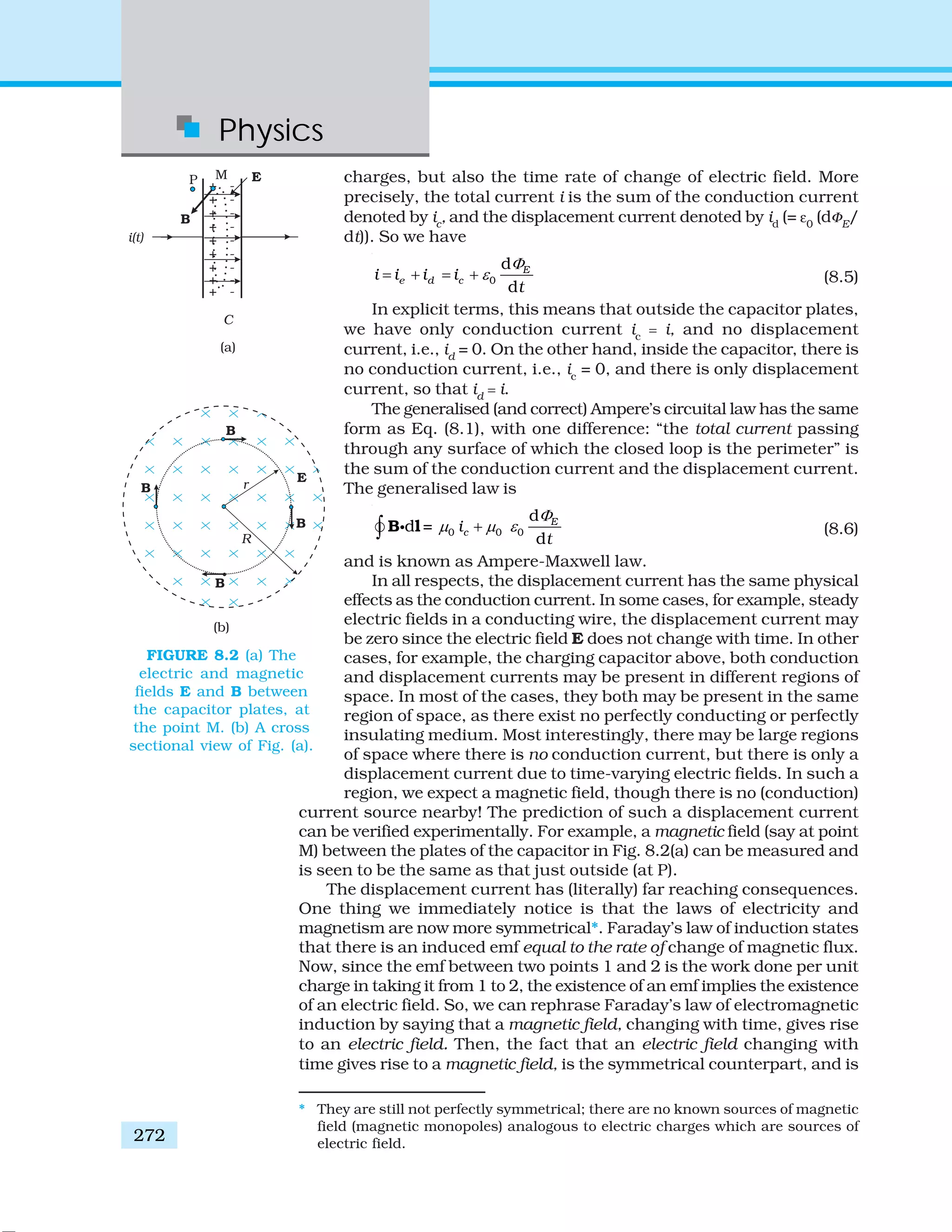
277. Electromagnetic
Waves
273
EXAMPLE8.1
a consequence of the displacement current being a source of a magnetic
field. Thus, time- dependent electric and magnetic fields give rise to each
other! Faraday’s law of electromagnetic induction and Ampere-Maxwell
law give a quantitative expression of this statement, with the current
being the total current, as in Eq. (8.5). One very important consequence
of this symmetry is the existence of electromagnetic waves, which we
discuss qualitatively in the next section.
MAXWELL’S EQUATIONS
1. 0d = /Q ε∫ E Ai (Gauss’s Law for electricity)
2. d =0∫ B Ai (Gauss’s Law for magnetism)
3.
B–d
d =
dt
Φ
∫ E li (Faraday’s Law)
4. 0 0 0
d
d =
d
E
ci
t
Φ
μ μ ε+∫ B li (Ampere – Maxwell Law)
Example 8.1 A parallel plate capacitor with circular plates of radius
1 m has a capacitance of 1 nF. At t = 0, it is connected for charging in
series with a resistor R = 1 MΩ across a 2V battery (Fig. 8.3). Calculate
the magnetic field at a point P, halfway between the centre and the
periphery of the plates, after t = 10–3
s. (The charge on the capacitor
at time t is q (t) = CV [1 – exp (–t/τ)], where the time constant τ is
equal to CR.)
FIGURE 8.3
Solution The time constant of the CR circuit is τ = CR = 10–3
s. Then,
we have
q(t) = CV [1 – exp (–t/τ)]
= 2 × 10–9
[1– exp (–t/10–3
)]
The electric field in between the plates at time t is
( )
0 0
q t q
E
Aε ε
= =
π
; A = π (1)2
m2
= area of the plates.
Consider now a circular loop of radius (1/2) m parallel to the plates
passing through P. The magnetic field B at all points on the loop is

278. Physics
274
along the loop and of the same value.
The flux ΦE
through this loop is
ΦE
= E × area of the loop
=
2
0
1
2 4 4
E q
E
ε
π⎛ ⎞
× π × = =⎜ ⎟⎝ ⎠
The displacement current
0
d
d
E
di
t
Φ
ε= ( )–61 d
0.5 10 exp –1
4 d
q
t
= = ×
at t = 10–3
s. Now, applying Ampere-Maxwell law to the loop, we get
( ) ( )0 0
1
2 0
2
c d dB i i iμ μ
⎛ ⎞
× π × = + = +⎜ ⎟⎝ ⎠ = 0.5×10–6
μ0
exp(–1)
or, B = 0.74 × 10–13
T
8.3 ELECTROMAGNETIC WAVES
8.3.1 Sources of electromagnetic waves
How are electromagnetic waves produced? Neither stationary charges
nor charges in uniform motion (steady currents) can be sources of
electromagnetic waves. The former produces only electrostatic fields, while
the latter produces magnetic fields that, however, do not vary with time.
It is an important result of Maxwell’s theory that accelerated charges
radiate electromagnetic waves. The proof of this basic result is beyond
the scope of this book, but we can accept it on the basis of rough,
qualitative reasoning. Consider a charge oscillating with some frequency.
(An oscillating charge is an example of accelerating charge.) This
produces an oscillating electric field in space, which produces an oscillating
magnetic field, which in turn, is a source of oscillating electric field, and
so on. The oscillating electric and magnetic fields thus regenerate each
other, so to speak, as the wave propagates through the space.
The frequency of the electromagnetic wave naturally equals the
frequency of oscillation of the charge. The energy associated with the
propagating wave comes at the expense of the energy of the source – the
accelerated charge.
From the preceding discussion, it might appear easy to test the
prediction that light is an electromagnetic wave. We might think that all
we needed to do was to set up an ac circuit in which the current oscillate
at the frequency of visible light, say, yellow light. But, alas, that is not
possible. The frequency of yellow light is about 6 × 1014
Hz, while the
frequency that we get even with modern electronic circuits is hardly about
1011
Hz. This is why the experimental demonstration of electromagnetic
wave had to come in the low frequency region (the radio wave region), as
in the Hertz’s experiment (1887).
Hertz’s successful experimental test of Maxwell’s theory created a
sensation and sparked off other important works in this field. Two
important achievements in this connection deserve mention. Seven years
after Hertz, Jagdish Chandra Bose, working at Calcutta (now Kolkata),
EXAMPLE8.1

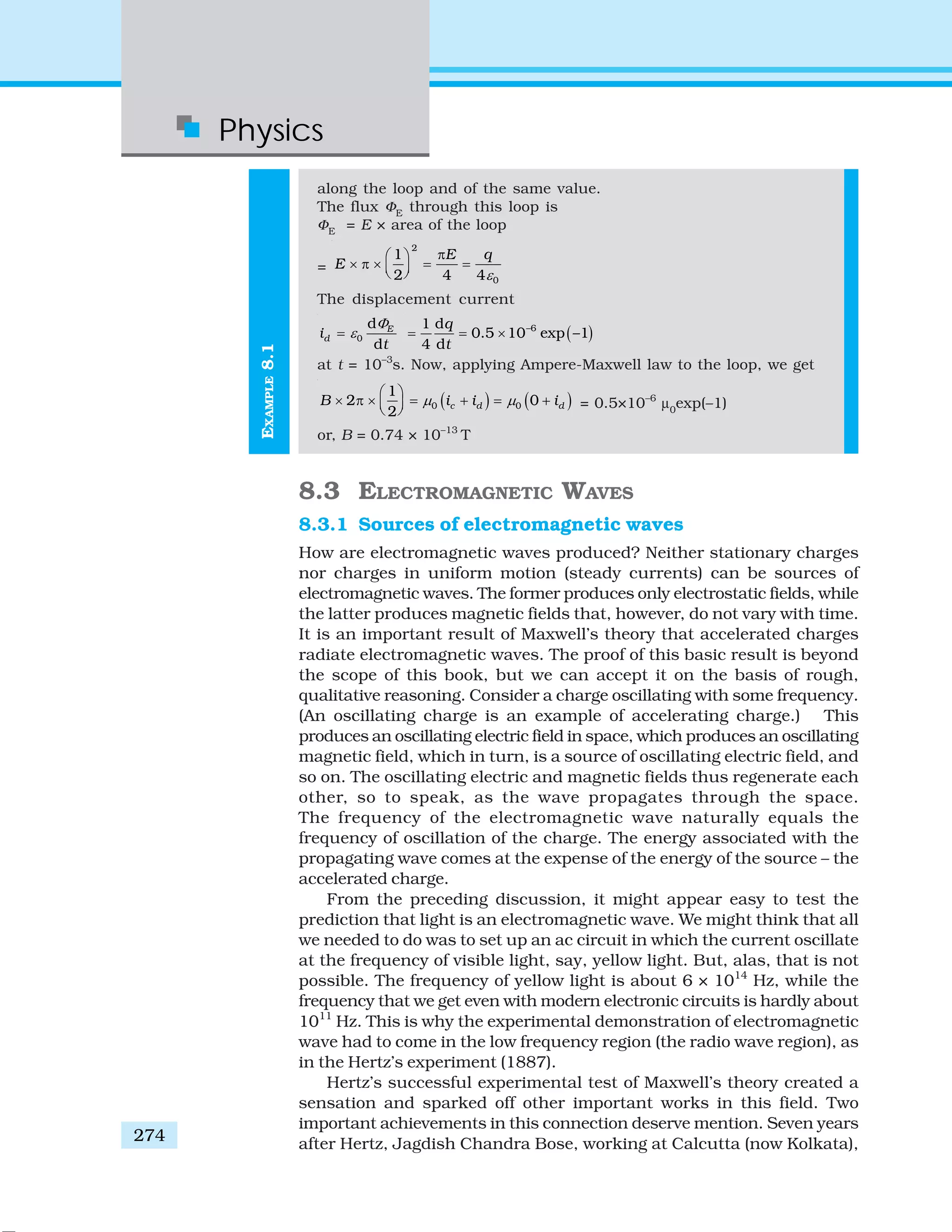
279. Electromagnetic
Waves
275
succeeded in producing and observing electromagnetic
waves of much shorter wavelength (25 mm to 5 mm).
His experiment, like that of Hertz’s, was confined to the
laboratory.
At around the same time, Guglielmo Marconi in Italy
followed Hertz’s work and succeeded in transmitting
electromagnetic waves over distances of many kilometres.
Marconi’s experiment marks the beginning of the field of
communication using electromagnetic waves.
8.3.2 Nature of electromagnetic waves
It can be shown from Maxwell’s equations that electric
and magnetic fields in an electromagnetic wave are
perpendicular to each other, and to the direction of
propagation. It appears reasonable, say from our
discussion of the displacement current. Consider
Fig. 8.2. The electric field inside the plates of the capacitor
is directed perpendicular to the plates. The magnetic
field this gives rise to via the displacement current is
along the perimeter of a circle parallel to the capacitor
plates. So B and E are perpendicular in this case. This
is a general feature.
In Fig. 8.4, we show a typical example of a plane
electromagnetic wave propagating along the z direction
(the fields are shown as a function of the z coordinate,
at a given time t). The electric field Ex
is along the x-axis,
and varies sinusoidally with z, at a given time. The
magnetic field By
is along the y-axis, and again varies
sinusoidally with z. The electric and magnetic fields Ex
and By
are perpendicular to each other, and to the
direction z of propagation. We can write Ex
and By
as
follows:
Ex
= E0
sin (kz–ωt) [8.7(a)]
By
= B0
sin (kz–ωt) [8.7(b)]
Here k is related to the wave length λ of the wave by the
usual equation
2
k
λ
π
= (8.8)
and ω is the angular frequency. k
is the magnitude of the wave
vector (or propagation vector) k
and its direction describes the
direction of propagation of the
wave. The speed of propagation
of the wave is (ω/k ). Using
Eqs. [8.7(a) and (b)] for Ex
and By
and Maxwell’s equations, one
finds that
Heinrich Rudolf Hertz
(1857 – 1894) German
physicist who was the
first to broadcast and
receive radio waves. He
produced electro-
magnetic waves, sent
them through space, and
measured their wave-
length and speed. He
showed that the nature
of their vibration,
reflection and refraction
was the same as that of
light and heat waves,
establishing their
identity for the first time.
He also pioneered
research on discharge of
electricity through gases,
and discovered the
photoelectric effect.
HEINRICHRUDOLFHERTZ(1857–1894)
FIGURE 8.4 A linearly polarised electromagnetic wave,
propagating in the z-direction with the oscillating electric field E
along the x-direction and the oscillating magnetic field B along
the y-direction.

280. Physics
276
ω = ck, where, c = 1/ 0 0μ ε [8.9(a)]
The relation ω = ck is the standard one for waves (see for example,
Section 15.4 of class XI Physics textbook). This relation is often written
in terms of frequency, ν (=ω/2π) and wavelength, λ (=2π/k) as
2
2 c
π
ν
λ
⎛ ⎞
π = ⎜ ⎟⎝ ⎠ or
νλ = c [8.9(b)]
It is also seen from Maxwell’s equations that the magnitude of the
electric and the magnetic fields in an electromagnetic wave are related as
B0
= (E0
/c) (8.10)
We here make remarks on some features of electromagnetic waves.
They are self-sustaining oscillations of electric and magnetic fields in free
space, or vacuum. They differ from all the other waves we have studied
so far, in respect that no material medium is involved in the vibrations of
the electric and magnetic fields. Sound waves in air are longitudinal waves
of compression and rarefaction. Transverse waves on the surface of water
consist of water moving up and down as the wave spreads horizontally
and radially onwards. Transverse elastic (sound) waves can also propagate
in a solid, which is rigid and that resists shear. Scientists in the nineteenth
century were so much used to this mechanical picture that they thought
that there must be some medium pervading all space and all matter,
which responds to electric and magnetic fields just as any elastic medium
does. They called this medium ether. They were so convinced of the reality
of this medium, that there is even a novel called The Poison Belt by Sir
Arthur Conan Doyle (the creator of the famous detective Sherlock Holmes)
where the solar system is supposed to pass through a poisonous region
of ether! We now accept that no such physical medium is needed. The
famous experiment of Michelson and Morley in 1887 demolished
conclusively the hypothesis of ether. Electric and magnetic fields,
oscillating in space and time, can sustain each other in vacuum.
But what if a material medium is actually there? We know that light,
an electromagnetic wave, does propagate through glass, for example. We
have seen earlier that the total electric and magnetic fields inside a
medium are described in terms of a permittivity ε and a magnetic
permeability μ (these describe the factors by which the total fields differ
from the external fields). These replace ε0
and μ0
in the description to
electric and magnetic fields in Maxwell’s equations with the result that in
a material medium of permittivity ε and magnetic permeability μ, the
velocity of light becomes,
1
v
με
= (8.11)
Thus, the velocity of light depends on electric and magnetic properties of
the medium. We shall see in the next chapter that the refractive index of
one medium with respect to the other is equal to the ratio of velocities of
light in the two media.
The velocity of electromagnetic waves in free space or vacuum is an
important fundamental constant. It has been shown by experiments on
electromagnetic waves of different wavelengths that this velocity is the
Simulatepropagationofelectromagneticwaves
(i)http://www.amanogawa.com/waves.html
(ii)http://www.phys.hawaii.edu/~teb/java/ntnujava/emWave/emWave.html

281. Electromagnetic
Waves
277
same (independent of wavelength) to within a few metres per second, out
of a value of 3×108
m/s. The constancy of the velocity of em waves in
vacuum is so strongly supported by experiments and the actual value is
so well known now that this is used to define a standard of length.
Namely, the metre is now defined as the distance travelled by light in
vacuum in a time (1/c) seconds = (2.99792458 × 108
)–1
seconds. This
has come about for the following reason. The basic unit of time can be
defined very accurately in terms of some atomic frequency, i.e., frequency
of light emitted by an atom in a particular process. The basic unit of length
is harder to define as accurately in a direct way. Earlier measurement of c
using earlier units of length (metre rods, etc.) converged to a value of about
2.9979246 × 108
m/s. Since c is such a strongly fixed number, unit of
length can be defined in terms of c and the unit of time!
Hertz not only showed the existence of electromagnetic waves, but
also demonstrated that the waves, which had wavelength ten million times
that of the light waves, could be diffracted, refracted and polarised. Thus,
he conclusively established the wave nature of the radiation. Further, he
produced stationary electromagnetic waves and determined their
wavelength by measuring the distance between two successive nodes.
Since the frequency of the wave was known (being equal to the frequency
of the oscillator), he obtained the speed of the wave using the formula
v = νλ and found that the waves travelled with the same speed as the
speed of light.
The fact that electromagnetic waves are polarised can be easily seen
in the response of a portable AM radio to a broadcasting station. If an
AM radio has a telescopic antenna, it responds to the electric part of the
signal. When the antenna is turned horizontal, the signal will be greatly
diminished. Some portable radios have horizontal antenna (usually inside
the case of radio), which are sensitive to the magnetic component of the
electromagnetic wave. Such a radio must remain horizontal in order to
receive the signal. In such cases, response also depends on the orientation
of the radio with respect to the station.
Do electromagnetic waves carry energy and momentum like other
waves? Yes, they do. We have seen in chapter 2 that in a region of free
space with electric field E, there is an energy density (ε0
E2
/2). Similarly,
as seen in Chapter 6, associated with a magnetic field B is a magnetic
energy density (B2
/2μ0
). As electromagnetic wave contains both electric
and magnetic fields, there is a non-zero energy density associated with
it. Now consider a plane perpendicular to the direction of propagation of
the electromagnetic wave (Fig. 8.4). If there are, on this plane, electric
charges, they will be set and sustained in motion by the electric and
magnetic fields of the electromagnetic wave. The charges thus acquire
energy and momentum from the waves. This just illustrates the fact that
an electromagnetic wave (like other waves) carries energy and momentum.
Since it carries momentum, an electromagnetic wave also exerts pressure,
called radiation pressure.
If the total energy transferred to a surface in time t is U, it can be shown
that the magnitude of the total momentum delivered to this surface (for
complete absorption) is,
U
p
c
= (8.12)

282. Physics
278
EXAMPLE8.3EXAMPLE8.2
When the sun shines on your hand, you feel the energy being
absorbed from the electromagnetic waves (your hands get warm).
Electromagnetic waves also transfer momentum to your hand but
because c is very large, the amount of momentum transferred is extremely
small and you do not feel the pressure. In 1903, the American scientists
Nicols and Hull succeeded in measuring radiation pressure of
visible light and verified Eq. (8.12). It was found to be of the order of
7 × 10–6
N/m2
. Thus, on a surface of area 10 cm2
, the force due to radiation
is only about 7 × 10–9
N.
The great technological importance of electromagnetic waves stems
from their capability to carry energy from one place to another. The
radio and TV signals from broadcasting stations carry energy. Light
carries energy from the sun to the earth, thus making life possible on
the earth.
Example 8.2 A plane electromagnetic wave of frequency
25 MHz travels in free space along the x-direction. At a particular
point in space and time, E = 6.3 ˆj V/m. What is B at this point?
Solution Using Eq. (8.10), the magnitude of B is
–8
8
6.3 V/m
2.1 10 T
3 10 m/s
E
B
c
=
= = ×
×
To find the direction, we note that E is along y-direction and the
wave propagates along x-axis. Therefore, B should be in a direction
perpendicular to both x- and y-axes. Using vector algebra, E × B should
be along x-direction. Since, (+ ˆj) × (+ ˆk ) = ˆi , B is along the z-direction.
Thus, B = 2.1 × 10–8 ˆk T
Example 8.3 The magnetic field in a plane electromagnetic wave is
given by By
= 2 × 10–7
sin (0.5×103
x+1.5×1011
t) T.
(a) What is the wavelength and frequency of the wave?
(b) Write an expression for the electric field.
Solution
(a) Comparing the given equation with
By
= B0
sin 2
x t
T
π
λ
⎡ ⎤⎛ ⎞
+⎜ ⎟⎢ ⎥⎝ ⎠⎣ ⎦
We get, 3
2
0.5 10
π
λ =
×
m = 1.26 cm,
and ( )111
1.5 10 /2 23.9 GHz
T
ν= = × π =
(b) E0
= B0
c = 2×10–7
T × 3 × 108
m/s = 6 × 101
V/m
The electric field component is perpendicular to the direction of
propagation and the direction of magnetic field. Therefore, the
electric field component along the z-axis is obtained as
Ez
= 60 sin (0.5 × 103
x + 1.5 × 1011
t) V/m

283. Electromagnetic
Waves
279
EXAMPLE8.4
Example 8.4 Light with an energy flux of 18 W/cm2
falls on a non-
reflecting surface at normal incidence. If the surface has an area of
20 cm2
, find the average force exerted on the surface during a 30
minute time span.
Solution
The total energy falling on the surface is
U = (18 W/cm2
) × (20 cm2
) × (30 × 60)
= 6.48 × 105
J
Therefore, the total momentum delivered (for complete absorption) is
p =
5
8
6.48 10 J
3 10 m/s
U
c
×
=
×
= 2.16 × 10–3
kg m/s
The average force exerted on the surface is
F =
3
6
4
2.16 10
1.2 10 N
0.18 10
p
t
−
−×
= = ×
×
How will your result be modified if the surface is a perfect reflector?
Example 8.5 Calculate the electric and magnetic fields produced by
the radiation coming from a 100 W bulb at a distance of 3 m. Assume
that the efficiency of the bulb is 2.5% and it is a point source.
Solution The bulb, as a point source, radiates light in all directions
uniformly. At a distance of 3 m, the surface area of the surrounding
sphere is
2 2 2
4 4 (3) 113mA r= π = π =
The intensity at this distance is
2
100 W 2.5 %Power
Area 113 m
I
×
= =
= 0.022 W/m2
Half of this intensity is provided by the electric field and half by the
magnetic field.
( )
( )
2
0
2
1 1
2 2
1
0.022 W/m
2
rmsI E cε=
=
( )( )12 8
0.022
V/m
8.85 10 3 10
rmsE −
=
× ×
= 2.9 V/m
The value of E found above is the root mean square value of the
electric field. Since the electric field in a light beam is sinusoidal, the
peak electric field, E0
is
E0
= rms2 2 2.9 V/mE = ×
= 4.07 V/m
Thus, you see that the electric field strength of the light that you use
for reading is fairly large. Compare it with electric field strength of
TV or FM waves, which is of the order of a few microvolts per metre.
EXAMPLE8.5

284. Physics
280
EXAMPLE8.5
Now, let us calculate the strength of the magnetic field. It is
1
8 1
2.9 V m
3 10 m s
rms
rms
E
B
c
−
−
= =
×
= 9.6 × 10–9
T
Again, since the field in the light beam is sinusoidal, the peak
magnetic field is B0
= 2 Brms
= 1.4 × 10–8
T. Note that although the
energy in the magnetic field is equal to the energy in the electric
field, the magnetic field strength is evidently very weak.
8.4 ELECTROMAGNETIC SPECTRUM
At the time Maxwell predicted the existence of electromagnetic waves, the
only familiar electromagnetic waves were the visible light waves. The existence
of ultraviolet and infrared waves was barely established. By the end of the
nineteenth century, X-rays and gamma rays had also been discovered. We
now know that, electromagnetic waves include visible light waves, X-rays,
gamma rays, radio waves, microwaves, ultraviolet and infrared waves. The
classification of em waves according to frequency is the electromagnetic
spectrum (Fig. 8.5). There is no sharp division between one kind of wave
and the next. The classification is based roughly on how the waves are
produced and/or detected.
FIGURE 8.5 The electromagnetic spectrum, with common names for various
part of it. The various regions do not have sharply defined boundaries.
Electromagneticspectrum
http://www.fnal.gov/pub/inquiring/more/light
http://imagine.gsfc.nasa.gov/docs/science/

285. Electromagnetic
Waves
281
We briefly describe these different types of electromagnetic waves, in
order of decreasing wavelengths.
8.4.1 Radio waves
Radio waves are produced by the accelerated motion of charges in conducting
wires. They are used in radio and television communication systems. They
are generally in the frequency range from 500 kHz to about 1000 MHz.
The AM (amplitude modulated) band is from 530 kHz to 1710 kHz. Higher
frequencies upto 54 MHz are used for short wave bands. TV waves range
from 54 MHz to 890 MHz. The FM (frequency modulated) radio band
extends from 88 MHz to 108 MHz. Cellular phones use radio waves to
transmit voice communication in the ultrahigh frequency (UHF) band. How
these waves are transmitted and received is described in Chapter 15.
8.4.2 Microwaves
Microwaves (short-wavelength radio waves), with frequencies in the
gigahertz (GHz) range, are produced by special vacuum tubes (called
klystrons, magnetrons and Gunn diodes). Due to their short wavelengths,
they are suitable for the radar systems used in aircraft navigation. Radar
also provides the basis for the speed guns used to time fast balls, tennis-
serves, and automobiles. Microwave ovens are an interesting domestic
application of these waves. In such ovens, the frequency of the microwaves
is selected to match the resonant frequency of water molecules so that
energy from the waves is transferred efficiently to the kinetic energy of
the molecules. This raises the temperature of any food containing water.
MICROWAVE OVEN
The spectrum of electromagnetic radiation contains a part known as microwaves. These
waves have frequency and energy smaller than visible light and wavelength larger than it.
What is the principle of a microwave oven and how does it work?
Our objective is to cook food or warm it up. All food items such as fruit, vegetables,
meat, cereals, etc., contain water as a constituent. Now, what does it mean when we say that
a certain object has become warmer? When the temperature of a body rises, the energy of
the random motion of atoms and molecules increases and the molecules travel or vibrate or
rotate with higher energies. The frequency of rotation of water molecules is about 300 crore
hertz, which is 3 gigahertz (GHz). If water receives microwaves of this frequency, its molecules
absorb this radiation, which is equivalent to heating up water. These molecules share this
energy with neighbouring food molecules, heating up the food.
One should use porcelain vessels and not metal containers in a microwave oven because
of the danger of getting a shock from accumulated electric charges. Metals may also melt
from heating. The porcelain container remains unaffected and cool, because its large
molecules vibrate and rotate with much smaller frequencies, and thus cannot absorb
microwaves. Hence, they do not get heated up.
Thus, the basic principle of a microwave oven is to generate microwave radiation of
appropriate frequency in the working space of the oven where we keep food. This way
energy is not wasted in heating up the vessel. In the conventional heating method, the vessel
on the burner gets heated first, and then the food inside gets heated because of transfer of
energy from the vessel. In the microwave oven, on the other hand, energy is directly delivered
to water molecules which is shared by the entire food.

286. Physics
282
8.4.3 Infrared waves
Infrared waves are produced by hot bodies and molecules. This band
lies adjacent to the low-frequency or long-wave length end of the visible
spectrum. Infrared waves are sometimes referred to as heat waves. This
is because water molecules present in most materials readily absorb
infrared waves (many other molecules, for example, CO2
, NH3
, also absorb
infrared waves). After absorption, their thermal motion increases, that is,
they heat up and heat their surroundings. Infrared lamps are used in
physical therapy. Infrared radiation also plays an important role in
maintaining the earth’s warmth or average temperature through the
greenhouse effect. Incoming visible light (which passes relatively easily
through the atmosphere) is absorbed by the earth’s surface and re-
radiated as infrared (longer wavelength) radiations. This radiation is
trapped by greenhouse gases such as carbon dioxide and water vapour.
Infrared detectors are used in Earth satellites, both for military purposes
and to observe growth of crops. Electronic devices (for example
semiconductor light emitting diodes) also emit infrared and are widely
used in the remote switches of household electronic systems such as TV
sets, video recorders and hi-fi systems.
8.4.4 Visible rays
It is the most familiar form of electromagnetic waves. It is the part of the
spectrum that is detected by the human eye. It runs from about
4 × 1014
Hz to about 7 × 1014
Hz or a wavelength range of about 700 –
400 nm. Visible light emitted or reflected from objects around us provides
us information about the world. Our eyes are sensitive to this range of
wavelengths. Different animals are sensitive to different range of
wavelengths. For example, snakes can detect infrared waves, and the
‘visible’ range of many insects extends well into the utraviolet.
8.4.5 Ultraviolet rays
It covers wavelengths ranging from about 4 × 10–7
m (400 nm) down to
6 × 10–10
m (0.6 nm). Ultraviolet (UV) radiation is produced by special
lamps and very hot bodies. The sun is an important source of ultraviolet
light. But fortunately, most of it is absorbed in the ozone layer in the
atmosphere at an altitude of about 40 – 50 km. UV light in large quantities
has harmful effects on humans. Exposure to UV radiation induces the
production of more melanin, causing tanning of the skin. UV radiation is
absorbed by ordinary glass. Hence, one cannot get tanned or sunburn
through glass windows.
Welders wear special glass goggles or face masks with glass windows
to protect their eyes from large amount of UV produced by welding arcs.
Due to its shorter wavelengths, UV radiations can be focussed into very
narrow beams for high precision applications such as LASIK (Laser-
assisted in situ keratomileusis) eye surgery. UV lamps are used to kill
germs in water purifiers.
Ozone layer in the atmosphere plays a protective role, and hence its
depletion by chlorofluorocarbons (CFCs) gas (such as freon) is a matter
of international concern.

287. Electromagnetic
Waves
283
8.4.6 X-rays
Beyond the UV region of the electromagnetic spectrum lies the X-ray
region. We are familiar with X-rays because of its medical applications. It
covers wavelengths from about 10–8
m (10 nm) down to 10–13
m
(10–4
nm). One common way to generate X-rays is to bombard a metal
target by high energy electrons. X-rays are used as a diagnostic tool in
medicine and as a treatment for certain forms of cancer. Because X-rays
damage or destroy living tissues and organisms, care must be taken to
avoid unnecessary or over exposure.
8.4.7 Gamma rays
They lie in the upper frequency range of the electromagnetic spectrum
and have wavelengths of from about 10–10
m to less than 10–14
m. This
high frequency radiation is produced in nuclear reactions and
also emitted by radioactive nuclei. They are used in medicine to destroy
cancer cells.
Table 8.1 summarises different types of electromagnetic waves, their
production and detections. As mentioned earlier, the demarcation
between different region is not sharp and there are over laps.
TABLE 8.1 DIFFERENT TYPES OF ELECTROMAGNETIC WAVES
Type Wavelength range Production Detection
Radio > 0.1 m Rapid acceleration and Receiver’s aerials
decelerations of electrons
in aerials
Microwave 0.1m to 1 mm Klystron valve or Point contact diodes
magnetron valve
Infra-red 1mm to 700 nm Vibration of atoms Thermopiles
and molecules Bolometer, Infrared
photographic film
Light 700 nm to 400 nm Electrons in atoms emit The eye
light when they move from Photocells
one energy level to a Photographic film
lower energy level
Ultraviolet 400 nm to 1nm Inner shell electrons in Photocells
atoms moving from one Photographic film
energy level to a lower level
X-rays 1nm to 10–3
nm X-ray tubes or inner shell Photographic film
electrons Geiger tubes
Ionisation chamber
Gamma rays <10–3
nm Radioactive decay of the -do-
nucleus

288. Physics
284
SUMMARY
1. Maxwell found an inconsistency in the Ampere’s law and suggested the
existence of an additional current, called displacement current, to remove
this inconsistency. This displacement current is due to time-varying electric
field and is given by
0
d
d
di
t
Φ
ε Ε
=
and acts as a source of magnetic field in exactly the same way as conduction
current.
2. An accelerating charge produces electromagnetic waves. An electric charge
oscillating harmonically with frequency ν, produces electromagnetic waves
of the same frequency ν. An electric dipole is a basic source of
electromagnetic waves.
3. Electromagnetic waves with wavelength of the order of a few metres were
first produced and detected in the laboratory by Hertz in 1887. He thus
verified a basic prediction of Maxwell’s equations.
4. Electric and magnetic fields oscillate sinusoidally in space and time in an
electromagnetic wave. The oscillating electric and magnetic fields, E and
B are perpendicular to each other, and to the direction of propagation of
the electromagnetic wave. For a wave of frequency ν, wavelength λ,
propagating along z-direction, we have
E = Ex
(t) = E0
sin (kz – ω t )
= E0
sin 02 sin 2
z z t
t E
T
ν
λ λ
⎡ ⎤ ⎡ ⎤⎛ ⎞ ⎛ ⎞
π − = π −⎜ ⎟ ⎜ ⎟⎢ ⎥ ⎢ ⎥⎝ ⎠ ⎝ ⎠⎣ ⎦ ⎣ ⎦
B = By
(t) = B0
sin (kz – ω t)
= 0 0sin 2 sin 2
z z t
B t B
T
ν
λ λ
⎡ ⎤ ⎡ ⎤⎛ ⎞ ⎛ ⎞
π − = π −⎜ ⎟ ⎜ ⎟⎢ ⎥ ⎢ ⎥⎝ ⎠ ⎝ ⎠⎣ ⎦ ⎣ ⎦
They are related by E0
/B0
= c.
5. The speed c of electromagnetic wave in vacuum is related to μ0
and ε0
(the
free space permeability and permittivity constants) as follows:
0 01/c μ ε= . The value of c equals the speed of light obtained from
optical measurements.
Light is an electromagnetic wave; c is, therefore, also the speed of light.
Electromagnetic waves other than light also have the same velocity c in
free space.
The speed of light, or of electromagnetic waves in a material medium is
given by 1/v μ ε=
where μ is the permeability of the medium and ε its permittivity.
6. Electromagnetic waves carry energy as they travel through space and this
energy is shared equally by the electric and magnetic fields.
Electromagnetic waves transport momentum as well. When these waves
strike a surface, a pressure is exerted on the surface. If total energy
transferred to a surface in time t is U, total momentum delivered to this
surface is p = U/c.
7. The spectrum of electromagnetic waves stretches, in principle, over an
infinite range of wavelengths. Different regions are known by different

289. Electromagnetic
Waves
285
names; γ-rays, X-rays, ultraviolet rays, visible rays, infrared rays,
microwaves and radio waves in order of increasing wavelength from 10–2
Å
or 10–12
m to 106
m.
They interact with matter via their electric and magnetic fields which set
in oscillation charges present in all matter. The detailed interaction and
so the mechanism of absorption, scattering, etc., depend on the wavelength
of the electromagnetic wave, and the nature of the atoms and molecules
in the medium.
POINTS TO PONDER
1. The basic difference between various types of electromagnetic waves
lies in their wavelengths or frequencies since all of them travel through
vacuum with the same speed. Consequently, the waves differ
considerably in their mode of interaction with matter.
2. Accelerated charged particles radiate electromagnetic waves. The
wavelength of the electromagnetic wave is often correlated with the
characteristic size of the system that radiates. Thus, gamma radiation,
having wavelength of 10–14
m to 10–15
m, typically originate from an
atomic nucleus. X-rays are emitted from heavy atoms. Radio waves
are produced by accelerating electrons in a circuit. A transmitting
antenna can most efficiently radiate waves having a wavelength of
about the same size as the antenna. Visible radiation emitted by atoms
is, however, much longer in wavelength than atomic size.
3. The oscillating fields of an electromagnetic wave can accelerate charges
and can produce oscillating currents. Therefore, an apparatus designed
to detect electromagnetic waves is based on this fact. Hertz original
‘receiver’ worked in exactly this way. The same basic principle is utilised
in practically all modern receiving devices. High frequency
electromagnetic waves are detected by other means based on the
physical effects they produce on interacting with matter.
4. Infrared waves, with frequencies lower than those of visible light,
vibrate not only the electrons, but entire atoms or molecules of a
substance. This vibration increases the internal energy and
consequently, the temperature of the substance. This is why infrared
waves are often called heat waves.
5. The centre of sensitivity of our eyes coincides with the centre of the
wavelength distribution of the sun. It is because humans have evolved
with visions most sensitive to the strongest wavelengths from
the sun.
EXERCISES
8.1 Figure 8.6 shows a capacitor made of two circular plates each of
radius 12 cm, and separated by 5.0 cm. The capacitor is being
charged by an external source (not shown in the figure). The
charging current is constant and equal to 0.15A.
(a) Calculate the capacitance and the rate of charge of potential
difference between the plates.

290. Physics
286
(b) Obtain the displacement current across the plates.
(c) Is Kirchhoff’s first rule (junction rule) valid at each plate of the
capacitor? Explain.
FIGURE 8.6
8.2 A parallel plate capacitor (Fig. 8.7) made of circular plates each of radius
R = 6.0 cm has a capacitance C = 100 pF. The capacitor is connected to
a 230 V ac supply with a (angular) frequency of 300 rad s–1
.
(a) What is the rms value of the conduction current?
(b) Is the conduction current equal to the displacement current?
(c) Determine the amplitude of B at a point 3.0 cm from the axis
between the plates.
FIGURE 8.7
8.3 What physical quantity is the same for X-rays of wavelength
10–10
m, red light of wavelength 6800 Å and radiowaves of wavelength
500m?
8.4 A plane electromagnetic wave travels in vacuum along z-direction.
What can you say about the directions of its electric and magnetic
field vectors? If the frequency of the wave is 30 MHz, what is its
wavelength?
8.5 A radio can tune in to any station in the 7.5 MHz to 12 MHz band.
What is the corresponding wavelength band?
8.6 A charged particle oscillates about its mean equilibrium position
with a frequency of 109
Hz. What is the frequency of the
electromagnetic waves produced by the oscillator?
8.7 The amplitude of the magnetic field part of a harmonic
electromagnetic wave in vacuum is B0
= 510 nT. What is the
amplitude of the electric field part of the wave?
8.8 Suppose that the electric field amplitude of an electromagnetic wave
is E0
= 120 N/C and that its frequency is ν = 50.0 MHz. (a) Determine,
B0
,ω, k, and λ. (b) Find expressions for E and B.
8.9 The terminology of different parts of the electromagnetic spectrum
is given in the text. Use the formula E = hν (for energy of a quantum
of radiation: photon) and obtain the photon energy in units of eV for
different parts of the electromagnetic spectrum. In what way are
the different scales of photon energies that you obtain related to the
sources of electromagnetic radiation?
8.10 In a plane electromagnetic wave, the electric field oscillates
sinusoidally at a frequency of 2.0 × 1010
Hz and amplitude 48 V m–1
.

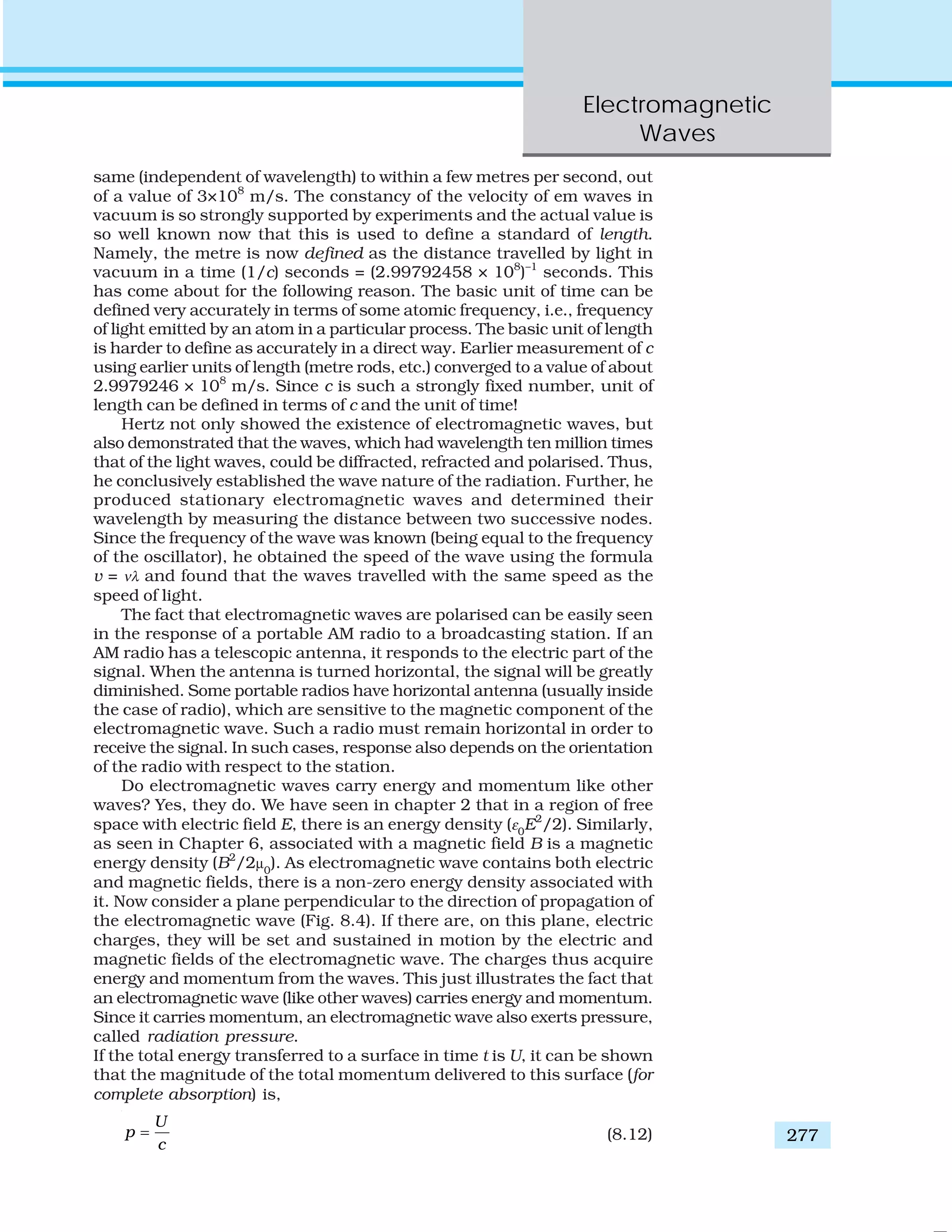
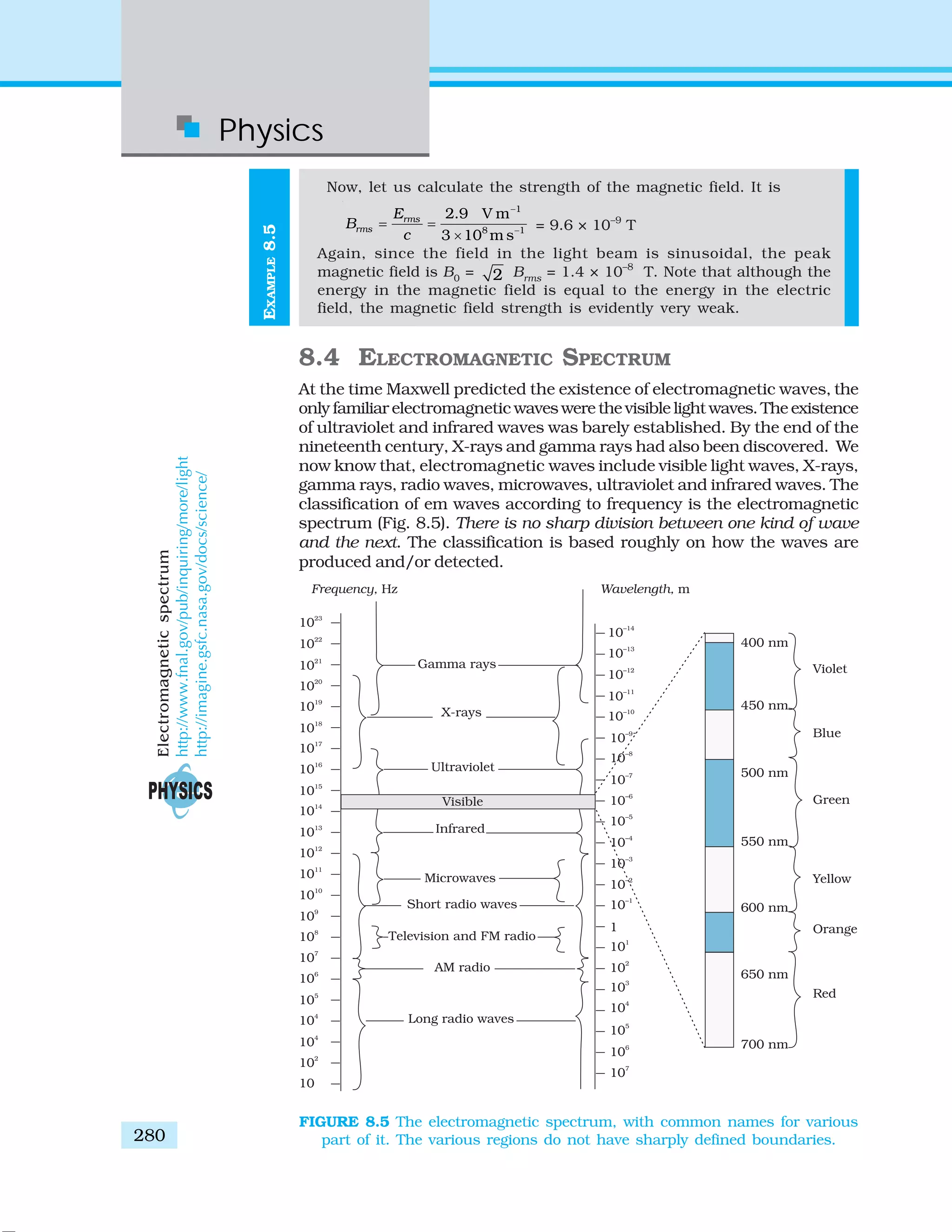
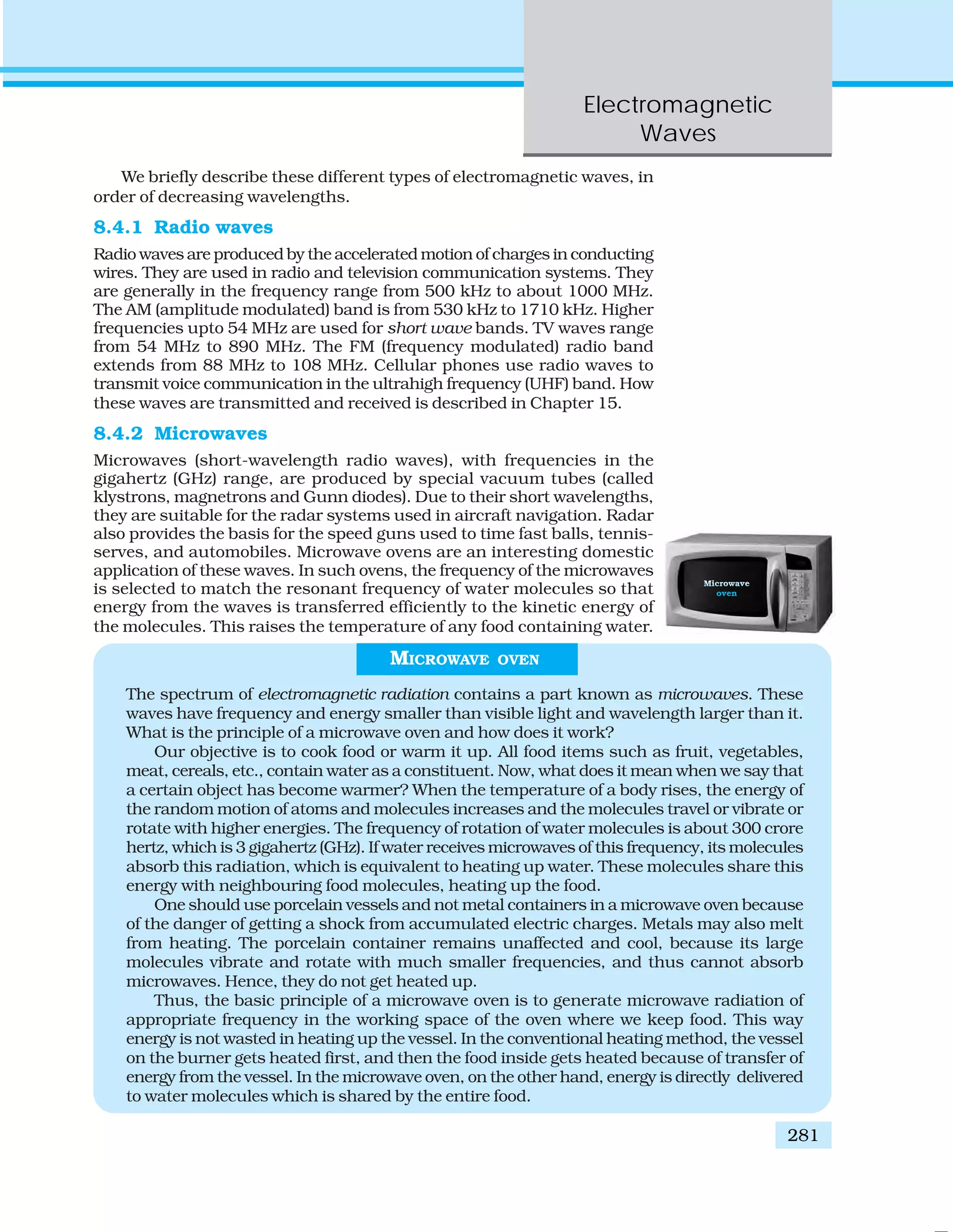
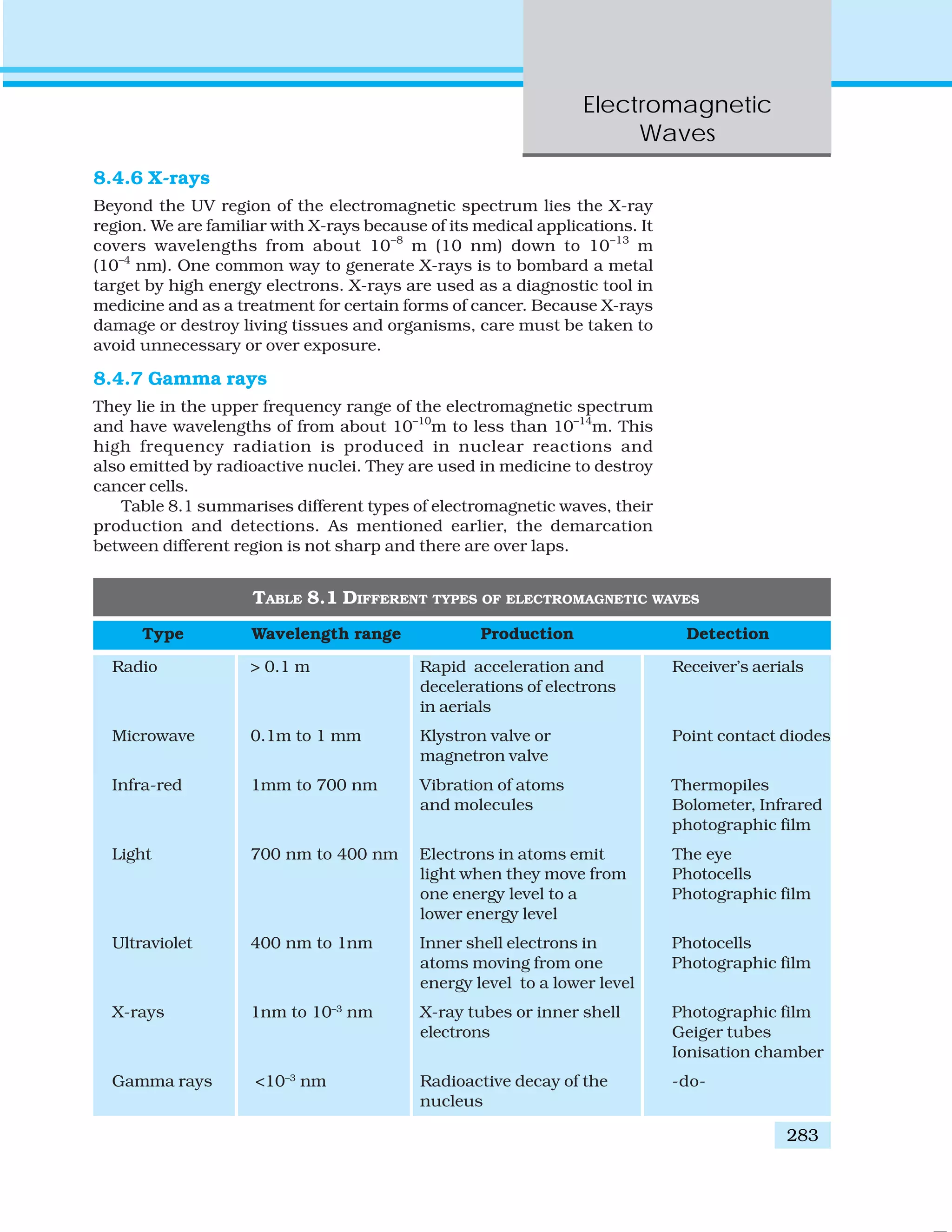
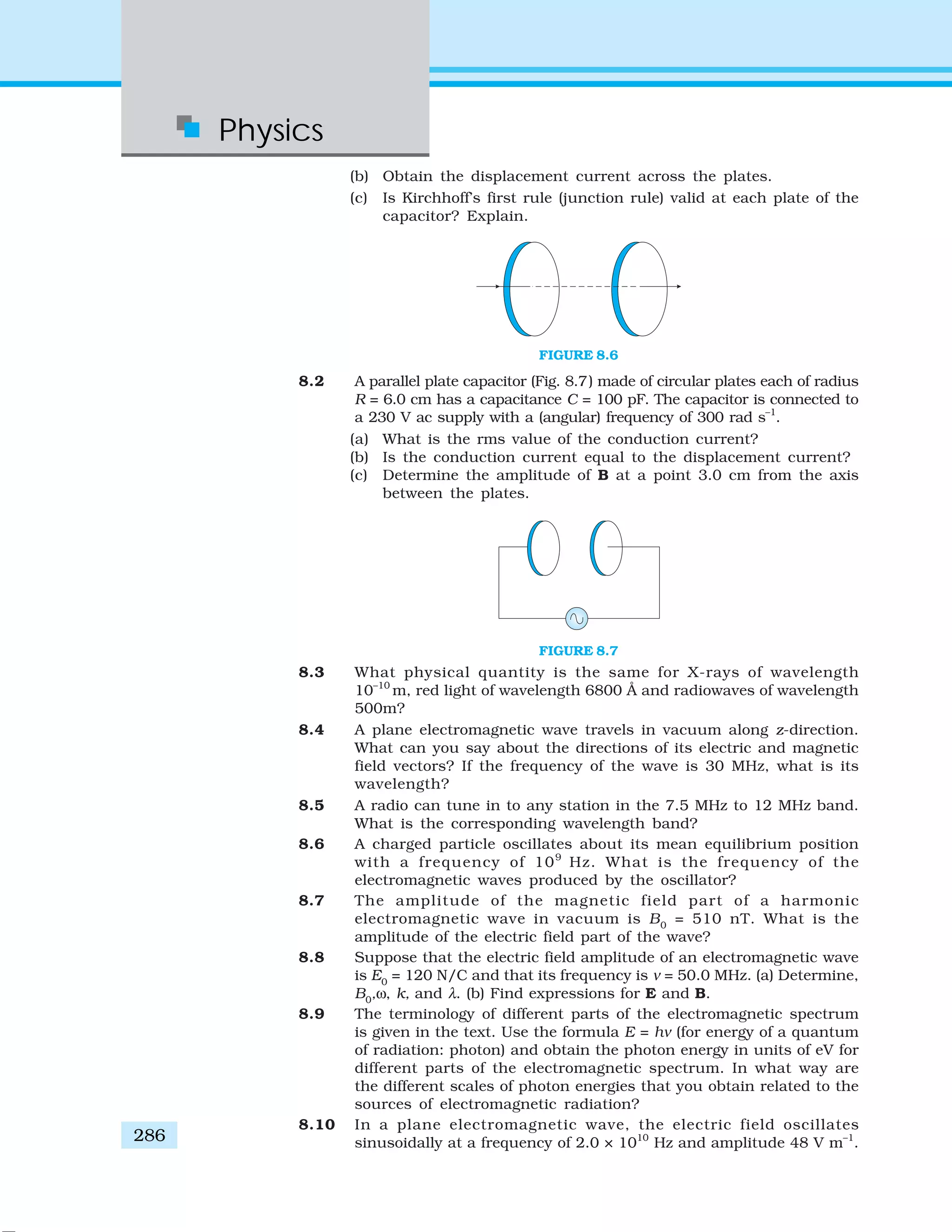
291. Electromagnetic
Waves
287
(a) What is the wavelength of the wave?
(b) What is the amplitude of the oscillating magnetic field?
(c) Show that the average energy density of the E field equals the
average energy density of the B field. [c = 3 × 108
m s–1
.]
ADDITIONAL EXERCISES
8.11 Suppose that the electric field part of an electromagnetic wave in
vacuum is E = {(3.1 N/C) cos [(1.8 rad/m) y + (5.4 × 106
rad/s)t]} ˆi .
(a) What is the direction of propagation?
(b) What is the wavelength λ ?
(c) What is the frequency ν ?
(d) What is the amplitude of the magnetic field part of the wave?
(e) Write an expression for the magnetic field part of the wave.
8.12 About 5% of the power of a 100 W light bulb is converted to visible
radiation. What is the average intensity of visible radiation
(a) at a distance of 1m from the bulb?
(b) at a distance of 10 m?
Assume that the radiation is emitted isotropically and neglect
reflection.
8.13 Use the formula λm
T = 0.29 cm K to obtain the characteristic
temperature ranges for different parts of the electromagnetic
spectrum. What do the numbers that you obtain tell you?
8.14 Given below are some famous numbers associated with
electromagnetic radiations in different contexts in physics. State
the part of the electromagnetic spectrum to which each belongs.
(a) 21 cm (wavelength emitted by atomic hydrogen in interstellar
space).
(b) 1057 MHz (frequency of radiation arising from two close energy
levels in hydrogen; known as Lamb shift).
(c) 2.7 K [temperature associated with the isotropic radiation filling
all space-thought to be a relic of the ‘big-bang’ origin of the
universe].
(d) 5890 Å - 5896 Å [double lines of sodium]
(e) 14.4 keV [energy of a particular transition in 57
Fe nucleus
associated with a famous high resolution spectroscopic method
(Mössbauer spectroscopy)].
8.15 Answer the following questions:
(a) Long distance radio broadcasts use short-wave bands. Why?
(b) It is necessary to use satellites for long distance TV transmission.
Why?
(c) Optical and radiotelescopes are built on the ground but X-ray
astronomy is possible only from satellites orbiting the earth.
Why?
(d) The small ozone layer on top of the stratosphere is crucial for
human survival. Why?
(e) If the earth did not have an atmosphere, would its average
surface temperature be higher or lower than what it is now?
(f ) Some scientists have predicted that a global nuclear war on the
earth would be followed by a severe ‘nuclear winter’ with a
devastating effect on life on earth. What might be the basis of
this prediction?