SlideShare a Scribd company logo
1 of 244
Download to read offline
ARGON BUBBLE BEHAVIOR IN SLIDE-GATE TUNDISH NOZZLES
DURING CONTINUOUS CASTING OF STEEL SLABS
BY
HUA BAI
B.S., Beijing Institute of Aeronautics and Astronautics, 1983
M.S., Beijing Institute of Aeronautics and Astronautics, 1986
THESIS
Submitted in partial fulfillment of the requirements
for the degree of Doctor of Philosophy in Mechanical Engineering
in the Graduate College of the
University of Illinois at Urbana-Champaign, 2000
Urbana, Illinois
iii
ABSTRACT
Argon injection into a tundish nozzle is an efficient and widely employed method to
reduce nozzle clogging in the continuous casting process. It also affects casting operation and
product quality by changing the flow pattern in the nozzle and mold. The current work combines
mathematical modeling and experiments to investigate the argon bubble behavior in slide-gate
nozzles and to analyze phenomena related to product defects and operational problems during
the continuous casting of steel slabs. Water model experiments are performed to study bubble
formation behavior, including bubble size, frequency, mode and effects of variables such as
liquid velocity, gas injection flow rate, gas injection hole size and gas density. An analytical
model is developed to predict the average bubble size. Argon gas bubbles are predicted to be
1~5mm. This is larger than air bubbles in water, especially at low speed. Typical sizes are 1
~3mm. A three-dimensional finite difference model is developed to study the turbulent flow of
liquid steel and argon bubble in the slide-gate nozzles. Experiments are performed on a 0.4-scale
“water caster” to verify the model by comparing the model prediction with the measurements
using PIV (Particle Image Velocimetry) technology. A weighted average scheme for the overall
outflow is developed to quantify jet characteristics such as jet angle, jet speed, back flow zone
fraction, turbulence and biased mass flow. Swirl is generated at nozzle ports. The validated
model is employed to perform extensive parametric studies to investigate the effects of casting
operation conditions such as gas injection, slide-gate orientation, casting speed, gate opening and
bubble size and nozzle port design including port angle and port shape. The interrelated effects
of nozzle clogging, argon injection, tundish bath depth, slide gate opening and nozzle bore
diameter on the flow rate and pressure in tundish nozzles are quantified using an inverse model,
based on interpolation of the numerical simulation results. The results are validated with
measurements on operating steel continuous slab-casting machines, and presented for practical
conditions. Suggestions to improve argon injection practice are proposed based on the modeling
results. During ladle transitions and at other times when either casting speed or tundish level is
low, argon flow should be turned off or at least severely reduced. The optimum argon flow rate
required to avoid air aspiration in the nozzle is derived from the model.
iv
ACKNOWLEDGEMENTS
I would like to express my sincere gratitude to my advisor, Professor Brian G. Thomas
for his guidance, support and encouragement through the course of this work. I am very grateful
for the opportunity to work with him, and have learned a great deal from him, which is far more
than any course or textbook could ever teach me. I would also like to thank Professor Jonathan
Dantzig, Professor S. Pratap Vanka, Professor S. Balachandar for their consent to serve on my
dissertation committee. Additionally, I am indebted to them for their advice and many helpful
suggestions for this thesis.
I would like to thank the National Science Foundation (Grant #DMI-98-00274) and the
Continuous Casting Consortium at UIUC, including Allegheny Ludlum, (Brackenridge, PA),
Armco Inc. (Middletown, OH), Columbus Stainless (South Africa), Inland Steel Corp. (East
Chicago, IN), LTV Steel (Cleveland, OH), and Stollberg, Inc., (Niagara Falls, NY) for their
continued support of our research, Professor J. Mazumder for use of the high speed video
camera, AEA Technology for technical support on using CFX4.2 package and the National
Center for Supercomputing Applications (NCSA) at the UIUC for computing time on Origin
2000 supercomputers. Additional thanks are extended to technicians at LTV Steel for help with
the PIV measurements.
I would like to extend my thanks to my officemates and fellow students, both past and
present, Guowei Li, Keith Rackers, David Stone, David Creech, Jon Parkman, Alex Danissov,
Yuji Miki, Jie Min, Chensheng Li, Lan Yu, Ya Meng, Tiebiao Shi, Melody Langeneckert and
Sivaraj Sivaramakrishnan. Their company, geniality, helpfulness and friendship helped to make
these years an enjoyable, memorable and rewarding experience.
I would like to express my deepest appreciation to my wife Snow and my daughter Carrie
for their love, counsel, encouragement and understanding throughout this endeavor. I am also
very grateful to my parents, whose confidence in me has been a great source of energy and
inspiration for me.
v
TABLE OF CONTENTS
Page
LIST OF TABLES ………………………………………………….………………………..… ix
LIST OF FIGURES ………………………………………………….……………………..…… x
NOMENCLATURE………………………………………………….………………………… xv
CHAPTER 1. INTRODUCTION ……………………………………………………………….. 1
CHAPTER 2. BUBBLE FORMATION STUDY ………………………………………………. 6
2.1 Introduction ………………………………………………….……………………… 6
2.2 Literature Review ………………………………………………….…………………7
2.3 Water Model Experiments ………………………………………………….………..9
2.3.1 Experimental Apparatus and Procedure ………………….…………………9
2.3.2 Bubble Size in Stagnant Liquid …………………………………………...11
2.3.3 Bubble Size in Flowing Liquid …………………………………………... 11
2.3.4 Bubble Formation Mode …………………………………………….……13
2.3.5 Bubble Elongation Measurement …………………………………….……15
2.3.6 Contact Angle Measurement ………..……………………………….…….16
2.4 Mathematical Model to Predict Bubble Size …….………………………………..……….. 18
2.4.1 Forces Acting on a Growing Bubble ………………………...……………18
2.4.2 Two-Stage Model for Bubble Formation in Flowing Liquid …………….. 20
2.4.3 Comparing with Measurements ……...……………………………………24
2.5. Argon Bubble Sizes in Liquid Steel …………………………………………….… 25
2.5.1 Difference between Steel-Argon and Water-Air Systems ……………….. 25
2.5.2 Predicting Bubble Size in Tundish Nozzles ……………………………… 26
2.5.3 Discussion ………………………………………………….…………….. 28
vi
2.6 Summary ……………………………………………….………………………….29
CHAPTER 3. TWO-PHASE FLOW IN SLIDE-GATE NOZZLES …………………………50
3.1 Previous Work …………………………………………….……………………… 50
3.2 Model Formulation …………………………………………….………………… 52
3.2.1 Governing Equations ………………………………….………………… 52
3.2.2 Boundary Conditions ………………………………….……………… 55
3.2.3 Solution Method ………………………………….……………………..57
3.2.4 Typical Simulation Results ………………………………….………….. 58
3.2.5 Multiple Steady-State Solutions ………………………………….………60
3.2.6 Jet Characteristics ………………………………….……………………61
3.3 Model Validation ………………………………….……………………………….. 63
3.3.1 Water Model Experiments and PIV Measurements ……………………. 63
3.3.2 Flow Pattern Observations …………………………….………………… 65
3.3.3 Velocity Comparisons …………………………….……………………….66
3.4 Model Discussion …………………………….……………………………………67
3.4.1 Dispersed Bubble Assumption ……………….………………………… 67
3.4.2 Split-Jet Calculation ………………….……………………………………68
3.5 Parametric Studies ……………….…………………………………………………70
3.5.1 Effect of Argon Gas Injection ….………………………………………….70
3.5.2 Effect of Slide-Gate Orientation ………………………………………….71
3.5.3 Effect of Casting Speed ……………….…………………………………75
3.5.4 Effect of Slide-Gate Opening ……….……………………………………77
3.5.5 Effect of Bubble Size ……………….…………………………………..78
3.5.6 Effect of Nozzle Port Design ……….………………………………… 78
vii
3.6 Pressure Drop across Nozzle …………….……………………………………… 80
3.7 Using Jet Solution in Mold Flow Modeling ……………………………………… 80
3.8 SUMMARY…..……………….………………………………………………………..82
CHAPTER 4. INTERRELATED EFFECTS OF CLOGGING, ARGON INJECTION
AND CASTING CONDITIONS………….…….……………………………...133
4.1 Introduction …….…………………………………………………………………133
4.2 Model Formulation ……….………………………………………………………134
4.2.1 Parametric Study with 3-D Finite Difference Model ……………………135
4.2.2 Multivariable Curve Fitting ……………………………………………136
4.2.3 Inverse Models .……...…………………………………………………139
4.2.4 Combined Model .………………………………………….……………142
4.3 Comparing with Plant Measurements …………………………………………143
4.4 Effect of Clogging .………………………………………………………………145
4.4.1 Initial Clogging and Edge Sharpness ………………………………145
4.4.2 Severe Clogging ……………………………………………………147
4.5 Effect of Air Aspiration …………………………………………………...………148
4.5.1 Lowest Pressure in Nozzle ……………………………………………148
4.5.2 Optimal Argon Flow ……………………………………………………150
4.6 Conclusions ………………………………………………………………………151
CHAPTER 5. CONCLUSIONS ……………………………………………………………172
5.1 Bubble Formation Study …..………………………………………………………172
5.2 Two-Phase Flow in Slide-Gate Nozzles …………………………………………174
5.3 Interrelated Effects of Clogging, Argon Injection and Casting Conditions ………176
viii
5.4 Mechanism for Argon Injection to Resist Nozzle Clogging ……………………177
CHAPTER 6. SUGGESTIONS FOR FUTURE WORK …………..………………………….179
APPENDIX A. SURFACE TENSION, CONTACT ANGLE AND WETTABILITY
IN BUBBLE FORMATION STUDY …………………………….….183
APPENDIX B. MATLAB PROGRAM TO CALCULATE THE BUBBLE SIZE
USING THE TWO-STAGE MODEL …………………………………..…189
APPENDIX C. CALCULATION OF ARGON GAS HEAT-UP THROUGH THE
HOLES IN NOZZLE WALL ………………………………………………193
APPENDIX D. DERIVATION OF EQUATION 4.1 ……………………………………… 198
APPENDIX E. DERIVATION OF THE INVERSE MODELS ……………………………200
APPENDIX F. MULTIVARIABLE CURVE FITTING MODEL FOR MINIMUM
PRESSURE IN NOZZLES ………………………………………………….206
APPENDIX G. SIMILARITY ANALYSIS FOR LIQUID STEEL-ARGON SYSTEM
AND WATER-AIR SYSTEM ……………………………………………….208
REFERENCE ...………………………………………………………………...…….….…..219
VITA ………………………………………………………………………….…....…………..225
ix
LIST OF TABLES
Page
Table 2.1 Average contact angles measured in the water experiments.……………..........31
Table 2.2 Physical properties and operating conditions used in the two-stage model …..31
Table 3.1 Nozzle dimension and operation conditions …………………………………….85
Table 3.2 Comparison of the overall average one-jet and the split-jet …………………… 86
Table 4.1 Simulation conditions for the standard nozzle……………………………..…...153
Table G.1 Physical properties used in the similarity analysis …………………...…..……209
Table G.2 Similarity requirements for liquid velocity, gas flow rate, and gas
volume fraction for full size water model ……………...……..………….….…212
Table G.3 Similarity requirement for gas flow rate and gas volume fraction
for the “mixed” dimensionless groups ………….………………..………….…213
Table G.4 Similarity requirement for gas flow rate in bubble formation study …………..216
x
LIST OF FIGURES
Page
Figure 1.1 Schematic of continuous casting tundish, slide-gate nozzle, and mold …….... 5
Figure 2.1 Schematic of water experiment for bubble formation study …………………….32
Figure 2.2 Measured air bubble sizes in stagnant water and prediction from
Iguchi's empirical correlation ………………………………………………… 33
Figure 2.3 Measured air bubble sizes under different gas injection flow rate and
water velocity and the effect of the modes to bubble size deviation to
their mean values …………………………………………………………..……34
Figure 2.4 Comparison of air bubble volumes in stagnant liquid and flowing liquid ………35
Figure 2.5 Figure 2.5 Effect of gas composition, gas flow rate and liquid velocity on
Bubble size……………………………………………………………… ………36
Figure 2.6 Photograph of the four bubble formation modes observed in experiments ……..37
Figure 2.7 Traced bubble formation process for two different modes …………………… 38
Figure 2.8 Photo series showing traced bubble formation process for two different modes..39
Figure 2.9 Bubble formation modes and their relation with liquid velocity and gas
injection flow rate ………………...…………………………………………… 40
Figure 2.10 Bubble elongation length at instant of bubble detachment from the gas
injection hole ….…………………………………………………………………41
Figure 2.11 Measured average elongation factor at bubble detachment (A)
and its extrapolation (B) ………………………………………………………42
Figure 2.12 Advancing and receding contact angles (A) and contact angle function
extrapolation (B) ...………………………………………………………………43
Figure 2.13 Schematic of forces acting on a growing bubble and liquid velocity
profile in nozzle in the expansion stage …………………………………………44
Figure 2.14 Evolution of vertical forces acting on a growing bubble with increasing
bubble size ………………………………………. ……………………………..45
Figure 2.15 Idealized sequence of bubble formation in the two stage model ………………46
Figure 2.16 Comparison of the predicted air bubble sizes in water with measurements….47
xi
Figure 2.17 Comparison of the predicted argon bubble diameters in liquid steel with
air bubble diameters in water …………………………………………………..48
Figure 2.18 Effect of the mean liquid velocity and gas flow rate on argon bubble in
liquid steel and air bubble in water ……………………………...………………49
Figure 3.1 Computational domain and boundary conditions for the standard nozzle ……..87
Figure 3.2 Grid resolution employed ……………………………………………………...88
Figure 3.3 Model predictions for various grid resolutions ………………………………...89
Figure 3.4 Convergence history for a typical 2-phase turbulence flow simulation run …...90
Figure 3.5 Simulated flow field for the standard nozzle and conditions in Table 3.1……..91
Figure 3.6 Predicted argon gas distribution for the standard nozzle and conditions
in Table 3.1 ……………………………………………………………….…....92
Figure 3.7 Predicted pressure distribution for the standard nozzle and conditions
In Table 3.1…………..……………………………………………………..……93
Figure 3.8 Predicted three vortex patterns for SEN under different initial conditions….…94
Figure 3.9 Photograph of the water experimental “water caster” ………………………...95
Figure 3.10 Schematic of PIV system ……………………………………………………96
Figure 3.11 Time history records of PIV measurements of the velocity components ……97
Figure 3.12 Predicted flow pattern and gas distribution at SEN port for PIV nozzle……..98
Figure 3.13 Effect of the upper edge port angle on back flow zone (y=3mm plane) ……….99
Figure 3.14 Flow pattern and jet photo showing vertical jet angle in water model
experiment ……………………………………………………………………...100
Figure 3.15 Comparison of PIV measurements and model prediction …………………….101
Figure 3.16 Vortex pattern at pot outlet and velocity profiles at different vertical slices
of the nozzle port …………………………………………………….….…….102
Figure 3.17 Effect of gas injection on gas volume fraction across nozzle bore on wide
face center plane (45° gate orientation, 8-44% gas, FL=50%,
VC=1m/min) …………………………………………………………….……103
xii
Figure 3.18 Flow pattern showing upward jet, downward jet and back flow zone on
port outlets of the standard nozzle (45° gate orientation, 28% gas,
FL=50%, VC=1m/min) …………………………………………………….….104
Figure 3.19 Effect of argon gas injection on flow pattern in nozzle ………………………105
Figure 3.20 Schematic of the slide-gate orientation (top view) and horizontal jet angle …106
Figure 3.21 Flow field at the center planes under different gate orientation ………………107
Figure 3.22 Flow field at the nozzle ports under different gate orientation ………………..108
Figure 3.23 Argon gas distribution in the standard nozzle with 0° gate orientation ……….109
Figure 3.24 Argon gas distribution in the standard nozzle with 45° gate orientation ………110
Figure 3.25 Argon gas distribution in the standard nozzle with 90° gate orientation……….111
Figure 3.26 Effects of slide-gate orientation and gas injection on vertical jet angle ……….112
Figure 3.27 Effects of slide-gate orientation and gas injection on horizontal jet angle……113
Figure 3.28 Effects of slide-gate orientation and gas injection on jet speed………………..114
Figure 3.29 Effect of slide-gate orientation and gas injection on back flow zone ………….115
Figure 3.30 Effect of slide-gate orientation and gas injection on biased mass flow………116
Figure 3.31 Effect of slide-gate orientation and gas injection on turbulence energy………117
Figure 3.32 Effects of casting speed and gas injection on vertical jet angle …………….….118
Figure 3.33 Effects of casting speed and gas injection on horizontal jet angle……………119
Figure 3.34 Effects of casting speed and gas injection on jet speed …………….………….120
Figure 3.35 Effects of casting speed and gas injection on back flow zone …………….….121
Figure 3.36 Effects of casting speed and gas injection on biased mass flow …………….…122
Figure 3.37 Effects of casting speed and gas injection on turbulence energy………….….123
Figure 3.38 Schematic of the definition of slide-gate opening for FL , FP and FA…………124
Figure 3.39 Relationship between different definitions for gate opening …………….….125
Figure 3.40 Effects of gate opening on jet characteristics…………….…………………….126
xiii
Figure 3.41 Effect of argon bubble size and gas injection on jet characteristics……………127
Figure 3.42 Liquid velocity fields superimposed on liquid volume fraction at center
plane and port under different nozzle port angles…………….………………128
Figure 3.43 Effect of the port angle on jet characteristics…………….…………………….129
Figure 3.44 Liquid velocity fields superimposed on liquid volume fraction at center
plane and port under different port shape designs …………….……………..130
Figure 3.45 Effect of the port shape design on jet characteristics…………….……………..131
Figure 3.46 Effects of gas injection and slide-gate orientation (A), casting speed (B),
and slide-gate opening (C) on pressure drop across the nozzle …….…………132
Figure 4.1 Pressure distribution in the standard nozzle, predicted by the 3-D finite
difference model (a) shaded contour plot at the center-plane (b) pressure
profile along the centerline (from top to outlet port) …………….…………..154
Figure 4.2 CFX data (points from Equation 4.1) and fitting curve (lines of
Equation 4.2) showing effects of casting speed VC, gate opening FL,
argon injection QG and nozzle bore size DN on tundish bath depth HT…………155
Figure 4.3 Inverse model plots showing effect of gate opening and tundish bath depth
on casting speed (A) Argon injection rate QG=0, and
(B) Argon injection rate QG=5 SLPM …………….…………………………..156
Figure 4.3 Inverse model plots showing effect of gate opening and tundish bath depth
on casting speed (C) Argon injection rate QG=10 SLPM…………….………157
Figure 4.4 Inverse model plots showing effect of gas injection and tundish bath depth
on casting speed…………….……………..…………………….……………158
Figure 4.5 CFX data (points) and fitting curve (lines) showing effects of casting
speed VC, gate opening FL, argon injection QG and nozzle bore size DN
on the lowest pressure PL in nozzle (under varying tundish bath depth) ………159
Figure 4.6 Comparison of the measurement and the model prediction…………….………160
Figure 4.7 Schematic of initial clogging and rounded edges in the vicinity of
the slide-gate (Validation Nozzle B) …………….…………………….……..161
Figure 4.8 Effects of initial clogging and rounded edges on tundish bath depth
(Validation Nozzle B) …………….……………………………….…………...162
Figure 4.9 Effects of initial clogging and rounded edges on nozzle flow pattern (center
plane parallel to the narrow face) for Validation Nozzle B …………….……163
xiv
Figure 4.10 Effects of clogging or nozzle bore size…………….……………..…………164
Figure 4.11 Effect of casting speed on minimum pressure in the nozzle for constant
tundish bath depth and argon injection flow rate (QG=10SLPM, DN=78mm)….165
Figure 4.12 Effect of casting speed on minimum pressure in the nozzle for constant
tundish bath depth and argon injection flow rate (QG=5SLPM, DN=78mm) …..166
Figure 4.13 Effect of casting speed on minimum pressure in the nozzle for constant
tundish bath depth and argon injection flow rate (QG=5SLPM, DN=70mm) …..167
Figure 4.14 Effect of argon injection flow rate on minimum pressure in the nozzle for
constant tundish bath depth and casting speed (VC=1m/min, DN=78mm) ……..168
Figure 4.15 Effect of argon injection flow rate on minimum pressure in the nozzle for
constant tundish bath depth and casting speed (VC=1.5m/min, DN=78mm) …..169
Figure 4.16 Effect of casting speed and tundish depth on minimum argon flow rate
required for positive pressure in nozzle (bottom) and the corresponding
gate opening (top) for DN=78mm …….……….……………………………..170
Figure 4.17 Effect of casting speed and tundish depth on minimum argon flow rate
required for positive pressure in nozzle (bottom) and the corresponding
gate opening (top) for DN=70mm ……………………………………..……..171
Figure A.1 Surface tension, contact angle and wettability…….……………………………187
Figure A.2 Contact angles at various points along the contact line between bubble and
solid surface for a bubble formed in transverse flowing liquid ……………188
Figure C.1 Schematic of the analytical model of argon gas heat-up through the nozzle
wall …………….…………………….…………………………………………193
Figure C.2 Numerical simulation of argon gas heat-up through the nozzle wall ………….197
Figure D.1 Schematic of the continuous casting process showing tundish, slide-gate
nozzle, mold and Location A, B, C, and D …………………………………….199
xv
NOMENCLATURE
ai, bi, ci, di curve fitting constant in Chapter 4 (i=1, 2, 3….)
CP specific heat (J/kg-K)
clg inter-phase momentum exchange coefficient
CD drag coefficient for bubble
D instantaneous equivalent bubble diameter (mm)
Db equivalent bubble diameter at detachment (mm)
DN diameter of nozzle bore (mm)
d gas injection hole diameter (mm)
E log-layer constant for velocity, 9.7930
e elongation factor
ed elongation factor at instant of bubble detachment
from gas injection hole(=L/Db)
FA slide-gate opening, area fraction opening of the slide-gate
FL slide-gate opening, linear fraction of the opening distance
FP slide-gate opening, linear fraction of plant definition
FB buoyancy force for a bubble (N)
FD drag force acting on a bubble, due to the flowing liquid (N)
Fr Froude number
FS surface tension force on a bubble (N)
FSz vertical component of surface tension force on a bubble (N)
f frequency of bubble formation from a gas injection hole (s-1
)
fl volume fraction for the liquid phase
fg volume fraction for the gas phase (“hot” for argon in steel)
xvi
fθ contact angle function, fθ =sinθΟ(cosθr-cosθa)
g gravitational acceleration (9.81m/s2
)
HT tundish bath depth (m)
HSEN SEN submerged depth (m)
h heat transfer coefficient (W/K-m2
)
K turbulence energy (m2
/ s2
)
K weighted average turbulent energy on nozzle port (m2
/ s2
)
k heat conductivity (W/m-K)
L (=edDb) elongation length at instant of bubble detachment (mm)
n distance normal to the wall, wall law (m)
N the number of measuring points (PIV) or computational cells (CFX) on the
laser light sheet on the nozzle port exit, Equation 3.26
PL lowest pressure in nozzle (kPa)
p pressure (kPa)
pl pressure for the liquid phase (kPa)
pg pressure for the gas phase (kPa)
QG “cold” argon gas flow rate, measured at standard conditions
(STP of 25˚C and 1 atmosphere pressure) (SLPM)
Qg gas injection flow rate per hole (ml/s)
QFe steel throughput (tonne/min)
r horizontal radius of the ellipsoidal bubble (mm)
re horizontal radius of the ellipsoidal bubble
at the end of the expansion stage (mm)
xvii
rd horizontal radius of the ellipsoidal bubble at the instant of bubble
detachment from the gas injection hole (mm)
rx, ry, rz, radii of the ellipsoidal bubble (rx =ry =r and , rz =eD ) (mm)
rzd vertical radius of the ellipsoidal bubble at detachment (mm)
Rebub Reynolds number for bubble Rebub=uD/υ
Ren Reynolds number for casting nozzle Ren=UDN/υ
Τ temperature (K)
TW wall temperature (K)
TO argon gas temperature at outer surface of the nozzle wall (K)
te time at the end of the expansion stage (s)
td time at the end of the detachment stage (s)
U average liquid velocity in nozzle (m/s)
UB average velocity at the top inlet of the nozzle (m/s)
UC average jet velocity at the nozzle port (m/s)
Ui liquid speed at cell i of the nozzle port (m/s)
Ujet jet speed (m/s)
u =u(y), liquid velocity profile across the nozzle bore (m/s)
u average liquid speed over the forming bubble (m/s)
ul weighted average liquid velocity at nozzle port in x-direction (m/s)
Vb bubble volume (=πD3
/6) (ml)
Ve bubble volume at the end of the expansion stage (ml)
VC casting speed for 8”x52” slab (m/min)
Vt velocity tangential to the wall, wall law (m/s)
vgi = { , , }
u v w
g g g , velocity components for gas phase (m/s)
xviii
vli = { , , }
u v w
l l l , velocity components for liquid phase (m/s)
vl weighted average liquid velocity at nozzle port in y-direction (m/s)
wl weighted average liquid velocity at nozzle port in z-direction (m/s)
We Weber number
x,y,z Cartesian coordinates (m)
y+
non-dimensional distance normal to the wall
y0
+
crossover point between the laminar sub-layer and the logarithmic region,
11.23
β gas volume expansion coefficient
∆p overall pressure-drop across the nozzle (kPa)
∆y length of the cell sides in the y direction (m)
∆z length of the cell sides in the z direction (m)
ε turbulent dissipation (m2
/ s3
)
ε weighted average turbulent dissipation at nozzle port (m2
/ s3
)
η back-flow zone fraction at nozzle port (m2
/ s3
)
κ Von-Karman constant, 0.419
µg molecule viscosity of the gas (kg/m-s)
µl molecule viscosity of the liquid (kg/m-s)
µt turbulent viscosity of the liquid (kg/m-s)
µeff effect kinetic viscosity of the liquid (kg/m-s)
θ contact angle ( °)
θo static contact angle ( °)
xix
θa advancing contact angle of a forming bubble( °)
θr receding contact angle of a forming bubble ( °)
θzx vertical jet angle (°)
θzx-slice slice jet angle (°)
θyx horizontal jet angle (°)
ρg density of the gas (kg/m3
)
ρl density of the liquid (kg/m3
)
σ surface tension coefficient of the liquid (N/m)
υ kinematic viscosity of the liquid =(µl /ρl) (m2
/s)
1
CHAPTER 1. INTRODUCTION
Continuous casting has been in industrial use for over thirty years and is the predominant
way by which steel is produced today in the world. A schematic of part of the typical continuous
slab-casting process is depicted in Figure 1.1 [1], showing the tundish, tundish nozzle and mold
regions. In a typical slab casting operation, the liquid steel flows from the tundish, through the
ceramic tundish nozzle, and exits through bifurcated ports into the liquid pool in the mold. The
tundish nozzle consists of the upper tundish nozzle (UTN), the slide-gate plates and the
submerged entry nozzle (SEN). Between these two nozzle segments, the flow rate is regulated by
moving a” slide gate”, which restricts the opening. Argon bubbles are injected through holes or
pores in the nozzle wall to mix into the flowing liquid steel. The nozzle outlet ports are
submerged below the surface of the molten steel in the mold to avoid interference with the
interface between the steel and the slag layers which float on top. The liquid steel in the mold
solidifies against the wall of the water-cooled, copper mold. The solidified steel shell acts as a
container for the molten steel as it is continuous withdrawn from the mold at a “casting speed”
and grows in thickness as it travels down below the mold. The completely solidified slab is then
cut into desired lengths by torches.
The quality of the continuous cast steel slab is greatly affected by the flow pattern in the
mold, which depends mainly on the flow pattern in the tundish nozzle, specifically the jets from
the nozzle port outlets. The flow pattern not only has a great influence on heat transfer to the
solidifying shell, but also governs the motion of inclusion particles and surface waves at the
meniscus, which affects the internal cleanness and quality of the steel. The tundish nozzle should
deliver steel uniformly into the mold while preventing problems such as surface waves, meniscus
freezing and crack formation. Impingement of hot liquid metal with high momentum against the
2
solidifying shell can contribute to shell thinning and even costly “breakouts”, where liquid steel
bursts from the shell [2]. In addition, the nozzle should be designed to deliver steel with the
optimum level of superheat to the meniscus while preventing both detrimental surface turbulence
and shell erosion or thinning due to excessive impingement of the hot molten steel jets. In some
operations, it is also important for the flow pattern to aid in the flotation of detrimental alumina
inclusions into the protective molten slag layer. Plant observations have found that many serious
quality problems are directly associated with nozzle operation and the flow pattern in the mold
[3]. For example, surface waves and turbulence near the top free surface can entrain some of the
slag into the steel flow, causing dangerous large inclusions and surface slivers [4]. The high
“standing wave” or large variation in the free surface level at the mold can prevent the liquid
mold flux from filling and lubricating the gap between the steel shell and the mold. This can
cause cracks in the steel shell due to thermal stresses and mold friction [5].
Nozzle clogging is one of the most disruptive phenomena on the operation of the tundish-
mold system. During the casting process, a buildup (clog) containing steel impurities may form
and deposit on the nozzle wall. This clog adversely affects product quality by changing the flow
pattern which is usually carefully designed, based on no-clogging condition, and by degrading
the internal quality of the final product when large chunks of it break off and enter the flow
stream. Also, as the buildup progresses, the slide gate opening must be increased to maintain the
desired flow rate. Once the slide-gate reaches its maximum position, production must stop and
the nozzle must be replaced.
Argon injection through the nozzle wall into the steel stream is an efficient and widely
employed method to reduce nozzle clogging, even though the real working mechanism is still not
fully understood [6]. However, the injected argon bubbles will also affect the flow pattern in the
nozzle, and subsequently in the mold. The argon bubbles might attach with small inclusions and
3
become entrapped in the solidifying shell, resulting in “pencil pipe” and blister defects on the
surface of the final product [7-10]. Other possible disadvantages of argon injection observed in
operation include increased quality defects and nozzle slag line erosion due to the increased
meniscus fluctuation [8, 11], exposure of the steel surface and subsequent reoxidation [12],
entrapment of the mold power [13]. Large gas injection flow rates might create a boiling action in
the mold [14, 15], which can greatly intensify those adverse effects. The boiling action at the mold
meniscus was experimentally found [16] related to a flow pattern change inside the tundish
nozzle, specifically, the regular “bubbly flow” changes to “annular flow” at high gas flow rate.
There is a great incentive to understand and predict the flow through the tundish nozzle
since tundish nozzle geometry is one of the few variables that is both very influential on the
continuous casting process and relatively inexpensive to change. Designing an effective nozzle
requires quantitative knowledge of the relationship between nozzle geometry and other process
variables on the flow pattern and the influential characteristics of the jet flow exiting the nozzle.
A well-designed nozzle with optimized argon injection implementation should meet the required
clogging-resistance capability, prevent the entrapment of those argon bubbles in solidified shell,
as well as provide desired flow patterns in both nozzle and mold, which hence help to achieve a
high quality cast slab.
The effect of gas injection on flow in the nozzle is relatively unstudied, especially
through mathematical modeling. Most previous works on modeling fluid flow in the nozzle have
focused on single-phase flow [1, 17-19]. A better understanding of fluid flow in the nozzle should
consider the effect of gas injection. Argon bubble motion and its effect on flow depends greatly
on the size of the bubbles which is determined during the initial stage of gas injection. Bubble
size is also an essential parameter for other advanced studies such as argon bubble motion [10],
4
inclusion attachment [10, 20], argon bubble and inclusion entrapment [9], in addition to modeling
liquid steel-argon bubble two-phase fluid flow in nozzle and mold [21-23].
This work investigates argon bubble behavior in slide-gate tundish nozzles during
continuous casting of steel slabs in three parts. First, water model experiments are performed to
study bubble formation behavior in flow conditions approximating those in a slide-gate tundish
nozzle of continuous casting process. The effects of liquid velocity, gas injection flow rate, gas
injection hole diameter, and gas density on bubble formation behavior such as bubble size,
injected gas mode are investigated. An analytical model is developed to predict the bubble size.
Secondly, a three-dimensional finite difference model is developed to study the liquid steel-
argon bubble two-phase turbulent flow in continuous casting tundish nozzles. Experiments are
performed on a 0.4-scale water model to verify the computational model by comparing its
prediction with velocity measurements using PIV (Particle Image Velocimetry) technology. A
weighted average scheme for the overall outflow is developed to quantify the characteristics of
the jets exiting the nozzle ports. Thirdly, the validated model is employed to perform extensive
parametric studies to investigate the effects of casting operation conditions and nozzle port
design. The interrelated effects of nozzle clogging, argon injection, tundish bath depth, slide gate
opening and nozzle bore diameter on the flow rate and pressure in tundish nozzles are quantified
using a inverse model, based on interpolation of the numerical simulation results. The results are
validated with measurements on operating steel continuous slab-casting machines, and presented
for practical conditions. Practical insights to optimize argon injection for various casting
conditions are presented.
This work is part of a larger project to develop and apply mathematical models to
understand and solve problems arising in the continuous casting process.
5
Submerged Entry Nozzle
(SEN)
Meniscus
Copper
Mold
AAA
AAA
AAA
AAA
AAA
AAA
AAA
AAA
AAA
AAA
AAA
AAA
AAA
AAA
AAA
AAA
Slide Gate
(flow control)
Submergence
Depth
Liquid Steel
Pool
Liquid Mold Flux
Solidifying Steel Shell
AA
AA
AA
AA
AA
AA
AA
AA
AA
AA
AA
AA
AA
AA
AA
AA
AA
AA
Continuous Withdrawal
Port Thickness
Port Height
Port Angle
Nozzle
Bore
Upper Tundish Nozzle
(UTN)
Molten Steel Jet
AAAAA
AAA
AAA
AAAAAAAAA
AAAAAAAAA
AAAAAAAAA
AAAAAAAAA
AAAAAAAAA
AAAAAAAAA
AAAAAAAAA
AAAAAAAAA
AAAAAAAAA
Tundish
AAAAAAAA
AAAAAAAA
AAAAAAAA
AAAAAAAA
AAAAAAAA
AAAAAAAA
AAAAAAAA
AAAAAAAA
AAAAAAAA
AAAAAAAAAAA
AAAAAAAAAAA
Liquid Steel
Protective
Slag Layer
AAAAAAAAAAA
Refractory Brick Steel Tundish Wall
AAA
AAA
AAA
AAA
AAA
AAA
Solid Mold Powder
AA
AA
AA
AA
AA
AA
AA
AA
A
A
A
AA
AA
AA
Argon Gas Injection
Figure 1.1 Schematic of continuous casting tundish, slide-gate nozzle, and mold [1]
6
CHAPTER 2. BUBBLE FORMATION STUDY
2.1 Introduction
Argon gas is injected through the walls of the ceramic nozzle into the liquid steel flow to
reduce clogging in a slide-gate nozzle. The injected argon bubbles affect the flow pattern in the
nozzle, and subsequently in the mold, thereby influencing the steel quality. Thomas et al. [22, 23],
modeled the liquid steel-argon bubble two-phase flow in mold, and found that argon bubble size
has an important effect that acts in addition to injection rate. Larger bubbles are found to leave
the mold faster and, therefore, have less influence on the liquid flow pattern in the mold. Small
bubbles travel with the jet further across the mold. Furthermore, small bubbles are more likely
penetrate deep into the liquid pool and become entrapped by the solidified shell, causing quality
problems, such as “pencil pipe” blister defects [10]. Creech [24] found that smaller bubbles
buoyed the jet and encouraged the transition from the classic ”double-roll” flow pattern in the
mold to “single-roll” for a given gas fraction. Wang et al. [20] found the optimal bubble size for
inclusion removal. Tabata et al. [25] performed water model tests of gas injection into the slide-
gate nozzle, and found that large bubbles tended to move to the center of the flow, thus lowering
their ability to catch inclusions and to prevent their adherence to the nozzle wall.
When argon gas is injected into a slide-gate nozzle through the pores (with typical
average diameter of 25~40µm) in the refractory material of the nozzle [6, 7, 26], or via machined
or laser cut holes (with typical diameter of 0.2~0.4mm) on the wall [6, 26, 27], the formation of
the bubbles is associated with the growth of a liquid-gas interface in an environment subjected to
the highly turbulent shearing flow of the liquid steel. The injected gas forms a succession of
bubbles which break away from the solid-liquid-gas interface, join the stream of the liquid steel,
7
and thereafter travel as separate entities in the liquid. Or, the injected gas may form a gas sheet
along the wall. This possibility is one of several suggested mechanisms for argon injection to
deter the clogging in nozzles [6, 11]. We want to know when each happen.
2.2 Literature Review
For bubble formation in liquid metals, some experimental works have been reported on
gas-stirred vessels in which gas is injected from an upward facing orifice or tube submerged in
quiescent liquid. The frequency of bubble formation was measured by using pressure pulse [28,
29], resistance probe [30, 31], or acoustic device [32]. The mean bubble sizes are then derived from
the known gas injection flow rate and the measured frequency of bubble formation. Efforts on
direct observation of bubble formation in liquid metal were also made by using X-ray
cinematography technique [33, 34]. Little work has been reported on bubble formation in flowing
liquid metals such as in tundish nozzles. Surface tension and contact angle between the gas,
liquid and solid surfaces is also very important to bubble formation. Recently, Wang et al [35]
studied the effect of wettability on air bubble formation using water model experiments in which
gas was injected through porous refractory into an acrylic tube with flowing water. Wettability as
changed by waxing the porous refractory. On the waxed surface, the bubbles tended to coalesce
together and form a gas curtain along the wall and then break into many uneven-sized bubbles
after travel certain distances. On an un-waxed surface, even-sized bubbles formed and detached
from the wall to join the liquid flow. No theoretical modeling work has been reported on bubble
formation in metallic systems.
On the other hand, extensive bubble formation studies have been done on aqueous
systems, both experimentally and theoretically, as reviewed by Kumar and Kuloor (1970) [36],
8
Clift et al. (1978) [37], Tsuge (1986) [38], and Rabiger and Vogelpohl (1986) [39]. Most of those
works are about bubble formation in stagnant liquid. The theoretical studies of bubble formation
can be divided into two categories: analytical spherical bubble models and discretized non-
spherical bubble models. The spherical bubble model assumes the spherical shape of the bubble
throughout the bubble growth. The bubble size at detachment is obtained by solving force
balance equation and/or bubble motion equation. The forces in equations are evaluated on the
whole growing bubble. Two of many significant contributions are the one-stage model by
Davidson and Schuler [40] and the two-stage model by Kumar and Kuloor [41]. The spherical
bubble models have to use empirical criteria for determining the instant of detachment. In
contrast, non-spherical bubble models have been developed [42-45] that are based on a local
pressure/force balance at the gas/liquid interface. In these models, the bubble surface is divided
into many two-dimensional axis-symmetric elements. For each element, two motion equations,
one in the radial direction and the other vertical direction, are solved to give its radial and
vertical velocities and then the position of the element. The bubble growth and bubble
detachment is determined by calculating the (non-spherical) shape of the bubble during its
formation. These models are therefore advantageous because they do not require the assumption
of bubble detachment criteria, but not applicable to asymmetric conditions such as with shearing
flowing liquid. Direct simulation of bubble formation process using CFD technology was
reported by Hong et al. [46] who numerically simulated the formation of a single bubble chain in
stagnant liquid by tracking the movement of the gas-liquid interface using the VOF (Volume of
Fluid) method [47].
Only a few works [48-50] were reported on bubble formation in flowing liquid condition.
In these models, the analytical spherical bubble models of bubble formation in stagnant liquid
are modified to accommodate the uniform liquid flow condition by including an additional drag
9
force due to the flowing liquid in the equation of motion. More empirical parameters are
introduced in order to match the experimental results, limiting the extension of these models to
different conditions.
None of these previous models can be directly applied to the current case -- bubble
formation in tundish nozzles, in which the gas is horizontally injected through the tiny holes on
the inner wall of the nozzle into highly turbulent downward-flowing liquid.
2.3 Water Model Experiments
Water model experiments are performed to investigate the bubble formation in flow
conditions that incorporate the essential phenomena in tundish nozzle flow. These include high
velocity flow of liquid along the wall, which shears the growing bubbles. Direct image
visualization and inspection are used to test the effects of liquid velocity, gas injection flow
rate, gas injection hole size, and gas composition on the bubble size, shape, frequency, and size
distribution. In addition to quantifying these important parameters, the results of these water
experiments also serve to validate the theoretical model developed later.
2.3.1 Experimental Apparatus and Procedure
Figure 2.1 shows a schematic of the water experimental apparatus. Water flows down
from an upper tank that simulates a tundish, through a vertical tube that simulates a tundish
nozzle, to a tank at the bottom that simulates a casting mold. The gas (air, helium, or argon) is
injected through a plastic tube attached to a hollow needle inserted horizontally into a square
35mm X 35mm Plexiglas tube. Water is made to flow vertically for conditions approximating
those in a tundish nozzle. The needle outlet is flush with the nozzle wall to simulate a pierced
hole on the inner wall of a nozzle. Three different-sized needles are used to examine the effect of
10
the gas injection orifice diameter (0.2, 0.3, and 0.4 mm). The gas flow controller is adjusted to
achieve volumetric gas flow rates of 0.17 ~ 6.0ml/s per orifice. Water flow rate is adjusted by
partially blocking the bottom of the nozzle. The average water velocity varies from 0.6m/s to
3.1m/s which corresponds to the pipe Reynolds number of 21,000 ~ 109,000.
The water velocity is obtained by measuring the average velocity of the tracing particles
that are purposely added to the water. The formation of bubbles is recorded by a high-speed
video camera at 4500 frames per second. Each recorded test contains 1000 frame images
accounting for 0.22 second measuring time. The head of liquid, defined as the vertical distance
between the top surface of the liquid in the upper tank to the needle, is about 500mm and drops
less than 20mm during video taping, owing to the short measurement time. The behavior of
bubbles exiting the needle is studied by inspecting the video images frame by frame. The
frequency (f) of bubble formation is determined by counting the number of the bubbles generated
at the exit of the injection needle during the recorded time period. The mean bubble volume (Vb)
is easily converted from the known gas injection volumetric flow rate (Qg), via
V
Q
f
b
g
= (2.1)
An equivalent average bubble diameter is calculated assuming a spherical bubble, or
D
Q
f
b
g
=






6
1 3
π
/
(2.2)
Bubbles sizes are also measured directly from individual video image in order to validate
this procedure and to check the bubble size deviation from its average value.
In some testing cases, a second needle is inserted into the nozzle wall 12.5mm
downstream the first needle in order to study the interaction between bubbles from the adjacent
gas injection sites.
11
2.3.2 Bubble Size in Stagnant Liquid
Experiments are first performed with stagnant water where previous measurements and
models are available for comparison. This was accomplished simply by closing the opening at
the bottom of the tube. Although most previous works are based on bubble formation from an
upward facing orifice or nozzle, some authors [32, 36] observed that the bubble sizes from a
horizontal orifice were almost the same as those from an upward facing orifice submerged in
stagnant liquid. Figure 2.2 shows the measured bubble diameters together with a prediction using
Iguchi’s empirical correlation [34].
It can be seen that bubble sizes increase with increasing gas injection flow rate. For the
same gas injection rate, a bigger injection orifice produces larger bubbles. At high gas injection
rate, larger bubbles emerge from larger diameter orifices. However, orifice size becomes less
important at small gas injection rate. The agreement between the experiment data and Iguchi’s
correlation prediction is reasonably good. This suggests that Iguchi’s empirical correlation,
which is based on relatively large gas injection flow rates and vertical injection, also applies to
the horizontal injection and relatively lower gas flow rates of this work.
2.3.3 Bubble Size in Flowing Liquid
Experiments are next performed with gas injection into flowing water. The measured
mean bubble sizes are plotted in Figure 2.3. Each point in Figure 2.3 represents the mean bubble
diameter for one test case with a particular gas injection flow rate, water velocity and gas
injection hole size. In addition, the maximum and minimum bubble sizes, obtained by directly
measuring the video images for the corresponding case, are shown as “error bars” for each point.
Also shown on the figure is the symbol (circle, triangle or square) representing the corresponding
mode that will be discussed later in this section.
12
Figure 2.3 shows that the mean bubble size increases with increasing gas flow rate and
decreasing water velocity. Comparing Figures 2.2 and 2.3, it can be seen that at the same gas
injection rate, the bubble size in flowing liquid is much smaller than in stagnant liquid. This
becomes much clearer when the bubble volumes for stagnant liquid and flowing liquid are
plotted together, as shown in Figure 2.4. Physically, the smaller bubble size in flowing liquid is
natural because the drag force due to the shearing liquid flow acts to shear the bubbles away
from the tip of the gas injection hole into the liquid stream before they grow to the mature sizes
found in stagnant liquid. The higher the velocity of the shearing liquid flow, the smaller the
detached bubbles are. The volumes of the bubbles formed in flowing water, in Figure 2.4, are
about 5 ~ 8 times smaller in volume than those in stagnant water.
All of the experimental data shown in Figures 2.3 and 2.4 are collected for air. Argon and
helium are also used in the experiments to investigate the effect of different gas composition.
Figure 2.5 shows that the measured mean bubble diameters for three different gases (air, argon
and helium) are about the same. Thus, the gas composition has little influence on bubble sizes.
It appears that bubble size is also relatively independent of gas injection hole size. This
can be seen when the mean bubble diameters in Figure 2.3 are re-plotted for fixed water velocity,
which is illustrated later as comparing with the model predictions in Figure 2.16. This
observation is different from that in stagnant liquid, where bubble size is larger for larger gas
injection hole. This suggests that the shearing force due to the flowing liquid dominates over
other effects related to the hole size such as surface tension force.
Figures 2.2-2.5 show that data collected with increasing water velocity generally also has
increasing gas flow. This choice of conditions was an unplanned consequence of the greater
water flow inducing lower pressure at the orifice, with consequently higher gas flow rate. The
higher-speed flowing liquid acts to aspirate more gas into the nozzle. This observation illustrates
13
the important relationship between liquid pressure and gas flow rate that should be considered
when investigating real systems.
2.3.4 Bubble Formation Mode
It is observed that the initial shape of the bubble exiting the gas injection hole falls into
one of four distinct modes, as shown in the representative recorded images of Figure 2.6. Figure
2.7 shows the series of outlines of two typical cases illustrating the formation process of bubbles,
corresponding to two different modes, based on tracing the recorded photo series shown in
Figure 2.8.
For low velocity water flows (less than 1m/s) and small gas injection rates (less than
2ml/s), Mode I is observed. In this mode, uniform-sized spherical bubbles form at the tip of the
gas injection hole. They elongate slightly before discretely detaching from the hole and joining
the liquid stream, as spherical bubbles again seen in Figure 2.7 top. There is no interaction
between the bubbles from the hole of the upper injection needle and the bubbles from the holes
of the lower needle if it exists.
At the other extreme, Mode IV is observed for high velocity water flows (more than
1.6m/s) and very large gas injection rates (more than 10ml/s). In this mode, each bubble
elongates down along the wall, forming a gas curtain, and the curtain merges with the gas from
the lower needle, if it exists, to form a long continuous gas curtain. The curtain eventually
becomes unstable when its thickness becomes too great and it breaks up into many different size
bubbles. Their size ranges from a few that are very large to others that are very tiny. For the
range of gas flow of practical interest, this regime is not expected.
Mode III is observed for high water flow conditions flows (more than 1.6m/s) and for
practical gas injection flow range (less than 6ml/s). Mode III is similar to Mode IV except that
14
there is insufficient gas flow to maintain a continuous gas curtain, so gaps form. Before
detaching from the gas injection hole, Figure 2.7 (bottom) documents that the bubbles elongate
about 2 times. The bubbles then elongate even more down along the wall and stay attached on
the wall for some distance after disconnecting from the gas injection hole.
Mode II is a transitional mode between Modes I and III in which the injected gas is
elongated along the wall but soon detaches from the wall. If a second gas injection hole exists,
the bubbles from the upper hole in Mode II will not coalesce with the bubbles from the lower
needle. Bubbles sizes in Mode II are still relatively uniform compared to those in Modes III and
IV.
In addition to the mean bubble size measured, Figure 2.3 also shows the mode and the
bubble size deviation from the mean value, using error bars to represent the size range for each
experimental case. All data under 0.9m/s water velocity fall into Mode I and have very small size
range, which corresponds to the relatively uniform spherical bubbles detaching near the tip of the
hole. This is similar to observation in stagnant liquid. Most data under 1.4m/s water velocity fall
into Mode II and have slightly larger size range. For the cases of liquid velocity at 1.9m/s and
2.5m/s, all of the data fall into Mode III and have huge size range, which corresponds to the
discontinuous gas curtain broken up into uneven-sized bubbles. The bubble size is as small as
0.5mm in diameter. The continuous gas curtain in Mode IV is observed only at very high gas
injection flow rate (Qg > 10 ml/s per hole), which is beyond the practical range of interest, so is
not shown in the plots.
For Mode III cases, no continuous gas curtain along the wall was observed for those
experiments with single needle gas injection. However, those elongated bubbles, after
disconnecting from the gas injection hole, still attach and travel along the wall for a certain
distance before they finally detach the wall and join the liquid stream, as seen in Figure 2.6 and
15
Figure 2.7 (Bottom). If they meet injected gas from the lower downstream hole before detaching
the wall, the two bubble streams coalesce to form larger elongated bubbles. In a real-life tundish
nozzle with hundreds of pierced holes or thousands of tiny pores on porous refractory, a
continuous gas curtain might be expected on the gas injection section of the inner wall of the
nozzle for Mode III. In fact, the argon gas injected into the liquid steel has much bigger tendency
to fall into Mode III and to form a gas curtain on the refractory wall due to the much larger
surface tension of the liquid steel and the non-wetting behavior of the liquid steel on the
refractory material. The experiments also show that no matter what bubble formation mode, the
injected gas will eventually detach from the wall, break up into discrete bubbles and join the
liquid stream. Therefore, there will be no gas curtain in the tundish nozzle after a certain distance
from the gas injection section.
It is found that when plotting each experimental data point with the ratio of gas flow rate
to mean liquid velocity (Qg/U) as y axis and the gas injection flow rate (Qg) as x axis, the
different bubble formation modes fall into separate regions, as shown in Figure 2.9.
2.3.5 Bubble Elongation Measurement
Bubble shape is observed to grow and elongate during the formation process. To quantify
the effects of the gas flow rate and liquid velocity on bubble elongation, the vertical elongation
length (L) is measured at the instant of the detachment of the bubble from its injection hole, as
shown in Figure 2.10(A). The measured bubble elongation lengths (L) are plotted in Figure
2.10(B). The effects become clear when plotting the elongation factor, ed, defined as the ratio of
the elongation length (L) and the equivalent diameter of the bubble (Db)
e
L
D
d
b
= (2.3)
16
As shown in Figure 2.11(A), the elongation factor mainly depends on liquid velocity, and is
relatively independent of the gas injection flow rate. Bubbles elongate slightly more at higher
liquid velocity. Figure 2.11(B) illustrates this effect of liquid velocity on the measured average
elongation factors. These four data points are well fitted with a simple quadratic function,
e = 0.78592+0.70797U - 0.12793U
d
2
(2.4)
which can be used to estimate the elongation factor at arbitrary liquid velocity rather than those
test velocities.
2.3.6 Contact Angle Measurement
Contact angles are measured for the purpose of evaluating the surface tension force,
which is used later in the model to predict bubble size. The relation between the contact angles
and surface tension force are detailed in Appendix A.
The static contact angle is defined by the profile adopted by a liquid drop resting in
equilibrium on a flat horizontal surface, and was measured to be 50° for the current water
experiment. The transverse flowing liquid makes the contact angles no longer uniform along the
bubble-solid contact circumference. At the upstream of the bubble, the contact angle increases to
θa, defined as the advancing contact angle, and at the downstream of the bubble, the contact
angle decreases to θr, defined as the receding contact angle, shown in Figures 2.12 (A).
Table 2.1 shows the measured mean contact angles in the water experiments. Generally
speaking, the advancing contact angle θa increases with increasing liquid velocity, and the
receding contact angle θr decreases with increasing liquid velocity. The effect of gas flow rate is
relatively small. Contact angle function, fθ, defined as
17
f o r a
θ θ θ θ
= −
( )
sin cos cos (2.5)
contains all contact angle terms in the surface tension force equation (Equation A.11),
In liquid steel-argon system, the surface tension force might have more influence on
bubble formation behavior due to significant increase in surface tension coefficient.
Unfortunately, except for the static contact angle, which is much larger for steel-argon system
(θO =150°) [54] than for water-air system (θO =50°), the advancing and receding contact angles
needed in Equation 2.5 are unknown due to lacking experimental data. Estimations on advancing
and receding contact angles can be made for elongated argon bubbles in flowing steel, based on
the observation in the air-water system. The advancing contact angle θa should be larger than the
static contact angle θO (150°) and increases with increasing liquid velocity, but it can not be
larger than 180°. The receding contact angle θr should be smaller than the static contact angle
and decreases with increasing liquid velocity. It is found from the estimations that the contact
angle function fθ might have close values for the steel-argon and water-air systems even though
all three contact angles (θO, θa and θr ) are very different between the two systems. For example,
if θa =155°(>θO =150°) and θr =124°(>θO =150°) , the contact angle function for the steel-argon
system will have the same value (fθ =0.30) as for the water-air system at liquid velocity
U=0.9m/s.
The contact angle function fθ increases with increasing liquid velocity, as shown in
Figure 2.12(B). The four data points are well fitted with a simple quadratic function,
f ( ) = -0.06079+0.33109U +0.078773U2
θ U (2.6)
18
Equation 2.6 can be used to estimate the value of the contact angle function at the liquid velocity
rather than those tests.
2.4 Mathematical Model to Predict Bubble Size
Bubble formation in vertical flowing liquid is very different from the classic bubble
formation problem in which the bubble forms at the end of an upward facing orifice or tube
submerged in stagnant liquid. In continuous casting process, argon gas is injected into the nozzle
horizontally through tiny holes on the inner wall of the nozzle. The injected gas encounters liquid
steel flowing downward across its path. The downward shearing liquid flow of interest to nozzle
injection is highly turbulent, with a Reynolds number of about 100,000. This turbulent flow
exerts a strong shear force on the forming bubble, which greatly affects its formation. Unlike
bubble formation in stagnant liquid, in which buoyancy force is the major driving force for
bubble detachment, the buoyancy force now acts to resist the premature detachment of the
bubble against the drag force of liquid momentum. Thus, previous bubble models can not be
directly applied. In developing an analytical model in this work for nozzle injection, the basic
ideas from the classic spherical bubble models in stagnant liquid are followed, which are based
on balancing the forces acting on the growing bubble and setting a proper bubble detachment
criteria.
2.4.1 Forces Acting on a Growing Bubble
Correct evaluation of the fundamental forces acting on the growing bubble is essential for
an accurate analytical model of bubble formation that can be extrapolated to other systems. A
schematic of the fundamental forces acting on a growing bubble is shown in Figure 2.13. The
forces of liquid drag, buoyancy, and surface tension are now discussed in turn.
19
Drag force due to flowing liquid FD
The drag force exerted by the flowing liquid onto the growing bubble, FD, depends on the
liquid velocity. The mean liquid velocity (U) in the nozzle is assumed to be known. Since the
growth and detachment of the bubble all occur near the wall and the shearing effect of the
flowing liquid creates small bubbles, the steep velocity gradient encountered by the forming
bubble are very important. This liquid velocity profile at the wall is needed for accurate
evaluation of the drag force. Of the many formulas for velocity profile of a fully developed
turbulent flow in a pipe, the most convenient for the current purpose is the seventh root law
profile [52]
u U
y
DN
=






1 235
2
1 7
.
/
/
(2.7)
where y is the distance from the wall, DN is the nozzle diameter, and U is the mean vertical
liquid velocity in the nozzle. The average liquid velocity across the growing bubble, u , depends
on the instantaneous bubble size and is estimated from
u
r
udy U
r
D
y
y r
N
= =
=
=
∫
1
2
1 3173
0
2
1 7
1 7
.
/
/
(2.8)
where r is the equivalent horizontal radius of the forming bubble. The drag force acting on the
growing bubble, FD, is
F C u r
D D l
=
1
2
2 2
ρ π (2.9)
Assuming the bubble Reynolds number, Rebub , is less than 3 105
× , the drag coefficient CD is[37]
CD
bub
bub bub
= + + + × −
24
1 0 15 0 42 1 4 25 10
0 687 4 1 16
Re
( . Re ) . / ( . Re )
. .
(2.10)
where Rebub is defined by
20
Rebub
uD
=
υ
(2.11)
where D is the equivalent bubble diameter and υ is the kinematic viscosity of the liquid.
Buoyancy force FB
Buoyancy force acts upward and resists the drag force due to the liquid momentum.
F V g D g
B b l g l g
= − = −
( ) ( )
ρ ρ π ρ ρ
1
6
3
(2.12)
Surface tension force FS
Surface tension force acts to keep the bubble attached to the wall. The vertical component
acts upward to resist drag of the bubble that elongates its shape below the gas injection hole, and
is given by [53].
F D
Sz O r a
= −
π
σ θ θ θ
4
sin (cos cos ) (2.13)
where σ is the surface tension coefficient. Derivation of Equation 2.13 is detailed in Appendix A.
The values for θO , θr and θa were measured from the video.
Figure 2.14 shows how those three fundamental forces change with the bubble size.
Other forces, such as the inertial force due to the rate of change of momentum of the growing
bubble, are believed to be negligible.
2.4.2 Two-Stage Model for Bubble Formation in Flowing Liquid
A two-stage model is developed to predict the size of the bubbles formed during nozzle
injection. The bubble formation is assumed take place in two idealized stages, the expansion
stage and the elongation stage, as shown in Figure 2.15.
21
Expansion stage
During the expansion stage, the forming bubble expands while holding onto the tip of the
gas injection. This stage is assumed to end when the downward forces are first able to balance
the upward force. That is,
F F F
D B Sz
= + (2.14)
The shape of the bubble during this stage is not considered until at the instant of the force
balance when it is assumed to be spherical. Substituting Equations 2.9, 2.12 and 2.13 into
Equation 2.14 yields
C u r r g r
D l l g O r a
1
2
4
3
1
2
2 2 3
ρ π π ρ ρ π σ θ θ θ
= − + −
( ) sin (cos cos ) (2.15)
In Equation 2.15, u depends on r, which is unknown in advance. Thus, Equation 2.15 is
solved for r by trial and error to yield re, which is the equivalent radius of the bubble at the end
of the expansion stage.
Elongation stage
As the bubble continues to grow, the downward force exceeds the upward forces on the
bubble. This makes the growing bubble begin to move downward along with the liquid flow. The
bubble keeps expanding since it still connects to the gas injection hole, and at the same time it
gets elongated due to the shearing effect of the liquid flow.
The shape of the bubble in the elongation stage is idealized as ellipsoidal. The connection
to the injection hole is assumed through a thin neck, thus the volume in the neck can be
neglected. The two horizontal radii of the ellipsoid (rx and ry ) are assumed to be the same to
simplify the problem, that is,
r r r
x y
= = (2.16)
22
and the vertical radius of the ellipsoid (rz ) accounts for the effect of the bubble elongation and is
related to the equivalent bubble diameter (D) and the elongation factor (e) by
r eD
z =
1
2
(2.17)
The elongation factor should match the measurement defined in Equation 2.3 at the instant of the
bubble detachment from its gas injection hole, or
r L e D
zd d b
= =
1
2
1
2
(2.18)
where rzd is the vertical radius of the ellipsoid bubble at the instant of the detachment.
The instantaneous equivalent diameter (D) of the bubble is related to the instantaneous
horizontal radius (r) of the ellipsoid and the instantaneous elongation factor (e) by
1
6
4
3
4
3
1
2
3 2 2
π π π
D r r r e D
z
= = 



or
D r e
= 2 (2.19)
The bubble gets more elongated as it grows bigger. The bottom of the ellipsoidal bubble
is assumed to travel along with the liquid at the average velocity u , defined in Equation 2.8.
Criterion to end this final stage of bubble growth is the detachment of the bubble from the gas
injection hole when the bubble elongates to the measured elongation at detachment. This
corresponds to the time when the vertical distance traveled by the fluid, from point A to B,
equals the critical length at the instant of bubble detachment, as shown in Figure 2.15(B).
udt e D
d
r
t
t
d b e
e
d
∫ = + −
2
(2.20)
Substituting Equation 2.19 into Equation 2.20 yields
udt r e
d
r
t
t
d d e
e
d
∫ = + −
2
2
3 2
/
(2.21)
23
where te and td are the bubble growing times at the end of the expansion stage and the instant of
bubble detachment respectively. rd is the horizontal radius at the detachment. The bubble
growing time (t) is related to the instantaneous horizontal radius of the growing ellipsoidal
bubble (r) by volume conservation, which assumes that pressure and temperature are sufficient
uniform to avoid compressibility effects.
Q t D
g =
1
6
3
π (2.22)
Substituting Equation 2.19 into Equation 2.22 yields
t
Q
r e
g
=
4
3
3 3 2
π /
(2.23)
Also knowing
e
at r r
e at r r
e
d d
=
=
=





1
(2.24)
the elongation factor at can be approximated by a linear function
e ar b at r r r
e d
= + < < (2.25)
The values of the constant a and b can be derived by satisfying the conditions in Equation 2.24:
a
e
r r
d
d e
=
−
−
1
(2.26)
b
r e r
r r
d d e
d e
=
−
−
(2.27)
From Equation 2.23 and Equation 2.25,
dt d
Q
r e
Q
r ar b
ar
ar b dr
g g
=





 = +
( ) + +
( )






4
3
4
2
3 3 2 2 3 2
3
1 2
π π
/ / /
(2.28)
Substituting Equation 2.8 and Equation 2.28 into Equation 2.21 yields
5 2692
2
1 7
2
3
1 2
1
7
3
2
1
7
. /
/
πU
Q D
r ar b
ar
ar b dr
g N r
r
e
d
+
( ) + +
( )






∫ = + −
2
2
3 2
r e
d
r
d d e
/
(2.29)
24
It should be noted that there are no adjustable parameters in this model. The elongation
factor at the instant of the bubble detachment (ed) and the contact angle function (fθ) depend on
the mean liquid velocity (U), and are obtained from the experimental measurements, shown in
Figures 2.11 and 2.12. To extend the model for the arbitrary liquid velocity beyond the test, the
extrapolated quadratic function, Equations 2.4 and 2.6, are used in the model.
Equation 2.29 are solved iteratively by trial and error for the horizontal radius of the
ellipsoidal bubble at the instant of detachment from the gas injection hole, rd, which is the only
unknown in this equation, using a program written in MATLAB detailed in Appendix B. The
equivalent bubble diameter is then converted from Equation 2.19 to
D r e
b d d
= 2 (2.30)
2.4.3 Comparing with Measurements
The bubble diameters predicted by the two-stage model are shown in Figure 2.16, along
with the measured mean bubble diameters. The physical properties of the fluids and operating
conditions used in calculation are summarized in Table 2.2
Figure 2.16 shows that the match between the model prediction and the experimental data
is reasonably good, although the predicted slopes (dD/dQg) appear to be slightly smaller than
experimental results. This means the model may slightly over-predict the bubble size for the low
gas injection flow rates and under-predict the bubble size for the high gas flow rates. Figure 2.16
shows the same trends of the effects of the liquid velocity and gas flow rate on bubble sizes as
observed during the experiments, that is, the mean bubble size increases with increasing gas
injection flow rate and decreasing shearing liquid velocity.
Figure 2.16 shows that the gas injection hole size rarely affects the bubble size at high
liquid velocity (U≥1.4m/s). This agrees with the water experiments that could hardly tell the
25
difference for the data measured from different hole sizes. However, at relatively low liquid
velocity, as shown in the plot for U=0.9m/s in Figure 2.16, the influence of the hole size
becomes slightly obvious, and the larger gas injection hole generates slightly larger bubbles. This
match the trends observed in the experiments for the stagnant liquid condition, which showed an
important effect of gas injection hole size on bubble size.
The two-stage model also predicts a negligible effect of the gas density that again
matches the experimental measurements. The gas density appears only in the buoyancy term in
the force balance Equation 2.15 in the form of (ρl-ρg), which is easy to see being negligible
compared with the liquid velocity.
There still exist some discrepancies between the predictions and measurements, as shown
in Figure 2.15. Random errors found in the experiments are likely one of the main sources. The
experiments were performed at highly turbulent flow conditions (experimental Reynolds
numbers range from 21,000 to 109,000), which is transient and random in nature. The recorded
1000 frame images for each case are for the period of only 0.22 second, which is not long
enough to make a good time average.
2.5. Argon Bubble Sizes in Liquid Steel
2.5.1 Difference between Steel-Argon and Water-Air Systems
In order to use the two-stage model developed above and validated for a water-air system
to predict the bubble size in the liquid steel-argon system in tundish nozzles, it is important to
understand the difference between the two systems. As seen in Table 2.2, there is big difference
in physical properties between the steel-argon system and water-air system. For example, the
surface tension coefficient for the liquid steel-argon system is more than 16 times of that of the
26
water-air system. The density of the liquid steel is 7 times of the water density. The effects of
these physical properties on bubble formation are incorporated in the two–stage model.
Except for the static contact angle, which is much larger for steel-argon system than for
water-air system [54], the advancing and receding contact angles needed in Equation 2.15 are
unknown for the liquid steel-argon system due to lacking experimental data. As discussed in
Section 2.3.6, the contact angle function fθ (=sinθο(cosθr-cosθa)) from the water experiment
might be close to the steel-argon system, thus adopted in calculation, as shown in Table 2.2.
Measurements [34] and calculation (Appendix C) show that gas injected through the “hot”
ceramic wall heats up to 99% of the liquid steel temperature even before it hits the liquid steel.
Thus, the argon gas injection flow rate used in the model is the “hot” argon flow rate.
2.5.2 Predicting Bubble Size in Tundish Nozzles
The two-stage model is used to predict argon bubble sizes in liquid steel in a typical
tundish nozzle with 78mm bore diameter. Air bubble sizes in water is also predicted for the same
conditions, as shown in the rightmost column of Table 2.2, for direct comparison. The
predictions are presented in Figure 2.17, showing the predicted bubble diameter vs. gas injection
flow rate under different liquid velocities. The argon bubble size increases with increasing gas
flow rate and decreasing liquid velocity, same trends as the air bubble size in water. In general,
argon bubbles generated in liquid steel are predicted to be larger than air bubbles in water. The
difference becomes more significant at lower liquid velocity and smaller gas flow rate. For the
practical interested range of the liquid velocity in tundish nozzles (0.7~1.2m/s), the difference in
bubble size between the two systems is sometimes significant. For example, a typical tundish
nozzle with 140 holes and 7 SLPM argon injection on UTN has 3.5 ml/s hot argon flow rate for
each hole. At the mean liquid velocity of 0.7m/s, the diameters of the argon bubbles in liquid
27
steel are about 1.5 times of those air bubbles in water, and the corresponding volumes of the
argon bubbles are 3.4 times of those of air bubbles.
The reason for larger bubbles predicted in the steel-argon system is mainly due to the
great difference in liquid density and surface tension coefficient in steel-argon system. This make
the drag force and surface tension force acting on the forming argon bubbles in liquid steel much
larger than those forces on the forming air bubble in water, under the same flow conditions.
Since the increase in surface tension force is more than two times of the increase in drag force,
the force balance of Equation 2.15 will be satisfied at a larger bubble size re at the end of the
expansion stage when compared to the water-air system. At very high liquid velocity, the drag
force due to the flowing liquid become so dominant that increase in surface tension force
becomes less important to the bubble formation behavior and thus the difference in bubble sizes
become smaller for the two systems.
Figure 2.18 plots the predicted bubble size for varying liquid velocity at a few fixed gas
flow rates for both systems. The two-stage model could not handle the very low liquid velocity
conditions. The program in Appendix B blowups at U<0.5m/s for water-air system and
U<0.7m/s for steel-argon system. Physically, this is because that at very low velocity downward
liquid flow, the downward drag force might not be able to balance the upward buoyancy force
and surface tension force. The bubble might go upward. The model need modification to deal
with the upward moving situation, in which the advancing contact angle and receding contact
angle switch positions and the surface tension force change its direction. The steel-argon system
blowups at higher liquid velocity due to its much higher surface tension than water-air system.
Since the ratio of the liquid and gas density for steel-argon system (ρl /ρg =104
) is one
order higher than for water-air system (ρl /ρg =103
), gas density should have no effect on argon
28
bubble size in liquid steel for the same reason as in water-air system. The effect of the gas
injection hole on argon bubble size is similar like air bubbles in water, although it is not plotted
here.
2.5.3 Discussion
The elongation factor and contact angle function fθ obtained from the water model
experiment, are directly employed for the tundish nozzle conditions due to lacking the
experimental data for liquid steel-argon system. The mean argon bubble size in liquid steel
predicted with the two-stage model is conservative or under-predicted due to the difference in
wettability. The non-wetting property of liquid metal on ceramics nozzle wall, in contrast to the
aqueous wetting system, makes the forming bubble tend to spread more over the wall, which has
been observed by other authors [32, 34, 35]. The spreading bubble might have a larger elongation
factor in this system. This will likely result in an under-predicted bubble size.
On the other hand, the tendency for argon bubbles to spread over the ceramics nozzle
wall makes the bubble formation mode fall into Mode II or III region at lower liquid velocity
than water-air system. Therefore, the argon bubbles should have larger tendency to have uneven
sizes when detaching from the wall.
The two-stage model predicts only the average bubble size, but not other important gas
bubble behavior such as bubble formation mode, bubble shape, bubble size deviation, bubble
coalescence and break-up. Direct numerical simulation of bubble formation process by tracking
the movement of the gas-liquid interface is a potential method to overcome these limitations.
Simulation of a single bubble chain in stagnant liquid using the VOF method has been reported
[46] to agree well with the experimental results in a real time sequence. However, numerical
29
simulation of argon bubble formation in a tundish nozzle condition is still a challenge, likely due
to the complex effects of turbulence, boundary layer, surface tension and wettability.
2.6 Summary
Water experiments are performed to study bubble formation from a horizontal oriented
hole facing a shearing downward turbulent liquid flow, approximating conditions in a tundish
nozzle. The effects of various parameters such as liquid velocity, gas injection flow rate, hole
diameter, and gas density on bubble formation behavior such as bubble size, injected gas mode
have been investigated. An analytical two-stage model based on force balance and bubble
formation sequence is developed to predict the bubble size at detachment from it gas injection
hole. Model predictions show good agreement with the measurements. The model is then used to
predict the size of the argon bubbles generated in liquid steel of a tundish nozzle. Specific
findings include:
• The mean bubble size increases with increasing gas injection flow rate.
• The mean bubble size increases with decreasing shearing liquid velocity.
• The mean bubble size in flowing liquid is significantly smaller than in stagnant liquid.
• The mean bubble size is relatively independent of gas injection hole size, especially at
high liquid velocity
• The gas composition has little influence on bubble size.
• Bubble formation falls into one of the four different modes, depending primarily on the
velocity of the flowing liquid and secondarily on the gas flow rate.
• In Mode I (low liquid speed and small gas flow rate), uniform-sized bubbles form and
detach from the wall. In Mode III (high liquid speed), the injected gas elongates down
along the wall and breaks into uneven sized bubbles. Mode II is intermediate between
30
Mode I and Mode III. In Mode IV (high liquid speed and high gas flow rate), the gas
elongates a long distance down the nozzle walls, forming a sheet before breaking up.
• Compared to water-air system, argon bubbles in liquid steel should tend to spread more
over the ceramic nozzle wall in liquid steel and fall into Mode II or III region. Thus, the
argon bubbles likely have a larger tendency to have non-uniform sizes when detaching
from the wall.
• Argon bubbles generated in liquid steel should be larger than air bubbles in water for the
same flow conditions. The difference should become more significant at lower liquid
velocity and smaller gas injection flow rate.
31
Table 2.1 Average contact angles measured in the water experiments
Average liquid
velocity (m/s)
Static
contact angle
θO (°)
Advancing
contact angle
θa (°)
Receding
contact angle
θr (°)
Contact angle function
fθ =sinθΟ(cosθr-cosθa)
0.9 50 64 35 0.30
1.4 50 82 29 0.56
1.9 50 101 22 0.85
2.5 50 134 27 1.26
Table 2.2 Physical properties and operating conditions used in the two-stage model
Parameters Symbol Unit
Water-Air
System for
matching
measurements
Steel-Argon
System
Water-Air
System for
comparison
Liquid density ρl
Kg m
/ 3
water:
1000
liquid steel:
7021
water:
1000
Gas density ρg
Kg m
/ 3
air:
1.29
hot argon:
0.27
air:
1.29
Liquid viscosity µl
kg/(ms) water:
0.001
liquid steel:
0.0056
water:
0.001
Gas viscosity µg
kg/(ms) air:
1.7E-5
hot argon:
7.42E-5
air:
1.7E-5
Surface tension
coefficient
σ N/m 0.073 1.192 0.073
Gas injection
flow rate/pore
Qg ml/s air:
0.1 ~ 6 ml/s
hot argon:
0.1 ~ 6 ml/s
air:
0.1 ~ 6 ml/s
Nozzle diameter Dn mm 35 78 78
Diameter of gas
injection hole
d mm 0.2, 0.3, 0.4 0.2, 0.3, 0.4 0.2, 0.3, 0.4
Average velocity
of the liquid
U m/s 0.9, 1.4,
1.9, 2.5
0.7, 0.9, 1.4
1.9, 2.5
0.7, 0.9, 1.4
1.9, 2.5
Elongation factor
at detachment
ed 1.32, 1.53,
1.67, 1.76
ed (U) = 0.78592
+ 0.70797U - 0.12793U2
Contact angle
function
sinθο(cosθr-cosθa)
fθ
0.30, 0.56
0.85, 1.26
fθ(U)= - 0.06079
+ 0.33109U + 0.078773U2
32
AAAAA
AAAAA
AAAAA
AAAAA
AAAAA
AAAAA
AAAAA
AAAAA
AAAAA
AAAAA
AAAAAAAAAAA
AAAAAAAAAAA
AAAAAAAAAAA
AAAAAAAAAAA
AAAAAAAAAAA
High-speed
video camera
Monitor
Recorder
Gas
source
flow
meter
Nozzle
Gas flow
controller
water velocity controller
Gas injection needle
Nozzle wall
Figure 2.1 Schematic of water experiment for bubble formation study
33
0
1
2
3
4
5
6
0 1 2 3 4 5
Iguchi (d=0.2)
Iguchi (d=0.3)
Iguchi (d=0.4)
measured (d=0.2)
measured (d=0.3)
measured (d=0.4)
Mean
bubble
diameter
(mm)
Gas injection flow rate (ml/s)
d: Gas injection hole diameter (mm)
Figure 2.2 Measured air bubble sizes in stagnant water and prediction
from Iguchi's empirical correlation [34]
34
0
0.5
1
1.5
2
2.5
3
3.5
0 1 2 3 4 5
Mode I
Mode II
Mode III
Bubble
diameter
(mm)
Gas injection flow rate (ml/s)
U=0.9m/s
U=1.4m/s
U=1.9m/s
U=2.5m/s
Gas inj. hole diameter d=0.4mm
0
0.5
1
1.5
2
2.5
3
3.5
0 1 2 3 4 5
Mode I
Mode II
Mode III
U=0.9m/s
U=1.4m/s
U=1.9m/s
U=2.5m/s
Gas injection flow rate (ml/s)
Bubble
diameter
(mm)
Gas inj. hole diameter d=0.3mm
0
0.5
1
1.5
2
2.5
3
3.5
0 0.5 1 1.5 2 2.5 3 3.5
Mode I
Mode II
Mode III
U=0.9m/s
U=1.4m/s
U=1.9m/s
U=2.5m/s
Gas injection hole diameter d=0.2mm
Bubble
diameter
(mm)
Gas injection flow rate (ml/s)
Figure 2.3 Measured air bubble sizes under different gas injection flow rate and water velocity
and the effect of the modes to bubble size deviation to their mean values
35
0
0.01
0.02
0.03
0.04
0 0.2 0.4 0.6 0.8 1 1.2 1.4
Flowing liquid (d=0.2)
Flowing liquid (d=0.3)
Flowing liquid (d=0.4)
Stagnant liquid (d=0.2)
Stagnant liquid (d=0.3)
Stagnant liquid (d=0.4)
Mean
bubble
volume
(ml)
Gas injection flow rate (ml/s)
Mean liquid velocity: 0.9m/s
Gas inj. hole diameter: d (mm)
Figure 2.4 Comparison of air bubble volumes in stagnant liquid and flowing liquid
36
0
0.5
1
1.5
2
2.5
3
0 0.5 1 1.5 2 2.5 3 3.5
U=0.9, Air
U=0.9, He
U=0.9, Ar
U=1.4, Air
U=1.4, He
U=1.4, Ar
U=1.9, Air
U=1.9, He
U=1.9, Ar
U=2.5, Air
U=2.5, He
U=2.5, Ar
U=0.9
U=1.4
U=1.9
U=2.5
Gas injection hole diameter d=0.2mm
Mean liquid velocity :U (m/s)
Gas injection flow rate (ml/s)
Mean
bubble
diameter
(mm)
Figure 2.5 Effect of gas composition, gas flow rate and liquid velocity on bubble size
37
Mode I Mode II Mode III Mode IV
Figure 2.6 Photograph of the four bubble formation modes observed in the experiments
38
AA
AA
AA
AA
AA
A
A
A
A
A
AA
AA
AA
AA
AA
A
A
A
A
A
AA
AA
AA
AA
AA
AA
AA
AA
AA
AA
A
A
A
A
A
AA
AA
AA
AA
AA
AA
AA
AA
AA
AA
A
A
A
A
A
AA
AA
AA
AA
A
A
A
A
AA
AA
AA
AA
A
A
A
A
A
AA
AA
AA
AA
AA
AA
AA
AA
AA
AA
A
A
A
A
A
AA
AA
AA
AA
AA
A
A
A
A
A
AA
AA
AA
AA
AA
Mode I (U=0.9m/s, QG=0.5ml/s, d=0.4mm), Bubble frequency f=293s-1
Equivalent bubble diameter: measured: 1.51mm, predicted: 1.53mm
Mode III (U=1.9m/s, QG=1.86ml/s, d=0.3mm), Bubble frequency f=444s-1
Equivalent bubble diameter: measured: 2.0mm, predicted:1.95mm
t=0 t=0.44ms t=0.89ms t=1.33ms t=1.78mm
t=2.22ms t=2.67ms t=3.11ms t=3.56ms t=4.00ms
t=0 t=0.44ms t=0.89ms t=1.33ms t=1.78mm
t=2.22ms t=2.67ms t=3.11ms t=3.56ms t=4.00ms
Figure 2.7 Traced bubble formation process for Mode I and Mode III
39
t=0 t=0.44ms t=0.89ms t=1.33ms t=1.78mm
t=2.22ms t=2.67ms t=3.11ms t=3.56ms t=4.00ms
t=0 t=0.44ms t=0.89ms t=1.33ms t=1.78mm
t=2.22ms t=2.67ms t=3.11ms t=3.56ms t=4.00ms
Mode I (U=0.9m/s, QG=0.5ml/s, d=0.4mm), Bubble frequency f=293s-1
Equivalent bubble diameter: measured: 1.51mm, predicted: 1.53mm
Mode III (U=1.9m/s, QG=1.86ml/s, d=0.3mm), Bubble frequency f=444s-1
Equivalent bubble diameter: measured: 2.0mm, predicted:1.95mm
Figure 2.8 Photo series showing the traced bubble formation process for Mode I and Mode III
40
0
0.5
1
1.5
2
2.5
0 1 2 3 4 5
Mode I
Mode II
Mode III
Gas
flow
rate
(ml/s)
/
Liquid
velocity
(m/s)
Gas injection flow rate (ml/s)
Figure 2.9 Bubble formation modes and their relation with liquid velocity
and gas injection flow rate
41
AA
AA
AA
AA
AA
AA
AA
L
Nozzle
wall
Q
g
Liquid flow
U
ed
=L/Db
0
1
2
3
4
5
6
0 1 2 3 4 5
U=2.5m/s
U=1.9m/s
U=1.4m/s
U=0.9m/s
Measured
elongation
length
(mm)
Gas injection flow rate (ml/s)
Gas injection hole diameter: d=0.4mm
Mean liquid velocity: U
(A) Schematic of the measurement (B) Measured elongations (L)
Figure 2.10 Bubble elongation length at instant of bubble detachment from the gas injection hole
42
0
0.5
1
1.5
2
0 1 2 3 4 5
U=2.5m/s
U=1.9m/s
U=1.4m/s
U=0.9m/s
Measured
elongation
factor
at
detachment
e
d
(=L/D)
Gas injection flow rate (ml/s)
Gas injection hole diameter: d=0.4mm
Mean liquid velocity: U
Ave. ed
=1.76
Ave. e
d
=1.67
Ave. ed
=1.53
Ave. ed
=1.32
(A)
0
0.5
1
1.5
2
0.5 1 1.5 2 2.5
Measured ave.
Curve-fitting
Elongation
factor
at
detachment
e
d
Mean liquid velocity U (m/s)
Curve-fitting model:
ed
= 0.78592+0.70797*U-0.12793*U2
Gas injection hole diameter: d=0.4mm
(B)
Figure 2.11 Measured average elongation factor at bubble detachment (A)
and its extrapolation (B)
43
θa
Liquid flow
θr
θa
θr
Liquid flow
Water-air system Steel-argon system
(A)
0
0.5
1
1.5
0.5 1 1.5 2 2.5
Measured ave.
Curve fitting
Curve-fitting model:
f
0
(U)=-0.06079+0.33109*U+0.078773*U2
Contact
angle
function
Mean liquid velocity U (m/s)
(B)
Figure 2.12 Advancing and receding contact angles (A)
and contact angle function extrapolation (B)
44
Liquid Velocity Profile u=u(y)
y 0
z
Gas
injection
Liquid Flow
Mean Velocity U
FB
FSZ
FS
FQ FSY
FD
Qg
Nozzle
wall
d
θr
θa
Figure 2.13 Schematic of forces acting on a growing bubble and
liquid velocity profile near wall region in the expansion stage
45
10-8
10
-7
10-6
10-5
10-4
10-3
10-2
0 0.5 1 1.5 2 2.5
Drag force F
D
Buoyancy force F
B
Surface tension force FSZ
Forces
acting
on
the
growing
bubble
(N)
Radius of a growing bubble (mm)
Mean liquid velocity U=0.9m/s
Gas injection hole dia. d=0.4mm
Figure 2.14 Evolution of vertical forces acting on a growing bubble with increasing bubble size
46
Liquid flow
U
Qg
Gas injection
Liquid flow
U
Qg
Gas
injection
2r
d
e
d
3/2
+d
/2
-r
e
L=D
b
e
d
=2
r
d
e
d
3/2
Nozzle
wall
Nozzle
wall
2rd
d/2
u(r)
2re
u(r)
A
B
z
y
2re
r
e
(A) Expansion stage (B) Elongation stage
Figure 2.15 Idealized sequence of bubble formation in the two stage model
47
0
0.5
1
1.5
2
2.5
0 0.2 0.4 0.6 0.8 1 1.2 1.4
d=0.4mm,measured
d=0.3mm,measured
d=0.2mm,measured
d=0.4mm,predicted
d=0.3mm,predicted
d=0.2mm,predicted
Mean
bubble
diameter
(mm)
Gas injection flow rate (ml/s)
Mean liquid velocity U=0.9m/s
d: Gas injection hole diameter
0
0.5
1
1.5
2
2.5
3
0 0.5 1 1.5 2 2.5
d=0.4mm,measured
d=0.3mm,measured
d=0.2mm,measured
d=0.4mm,predicted
d=0.3mm,predicted
d=0.2mm,predicted
Mean
bubble
diameter
(mm) Gas injection flow rate (ml/s)
Mean liquid velocity: 1.4m/s
d: Gas inj. hole diameter
0
0.5
1
1.5
2
2.5
3
0 0.5 1 1.5 2 2.5 3 3.5
d=0.4mm, measured
d=0.3mm, measured
d=0.2mm, measured
d=0.4mm, predicted
d=0.3mm, predicted
d=0.2mm, predicted
Mean
bubble
diameter
(mm)
Gas injection flow rate (ml/s)
Mean liquid velocity: 1.9m/s
d: Gas injection hole diameter
0
0.5
1
1.5
2
2.5
3
3.5
0 1 2 3 4 5
d=0.4mm, measured
d=0.3mm, measured
d=0.2mm, measured
d=0.4mm, predicted
d=0.3mm, predicted
d=0.2mm, predicted
Mean
bubble
diameter
(mm)
Gas injection flow rate (ml/s)
Mean liquid velocity: 2.5m/s
d: Gas injection hole diameter
Figure 2.16 Comparison of the predicted air bubble sizes in water with measurements
48
0
1
2
3
4
5
6
7
0 1 2 3 4 5 6
Steel-argon system
Water-air system
Mean
bubble
diameter
(mm)
Gas injection flow rate (ml/s)
Mean liquid velocity U=0.7m/s
Gas injection hole diameter d=0.3mm
0
1
2
3
4
5
6
7
0 1 2 3 4 5 6
Fe-Ar@U=0.9
Fe-Ar@U=1.4
W-Air@U=0.9
W-Air@U=1.4
Mean
bubble
diameter
(mm)
Gas injection flow rate (ml/s)
Gas injection hole diameter d=0.3mm
Fe-Ar: Liquidsteel-Argon system
W-Air: Water-Air system
U: Mean liquid velocity (m/s)
0
1
2
3
4
5
6
7
0 1 2 3 4 5 6
Fe-Ar@U=1.9
Fe-Ar@U=2.5
W-Air@U=1.9
W-Air@U=2.5
Mean
bubble
diameter
(mm)
Gas injection flow rate (ml/s)
Gas injection hole diameter d=0.3mm
Fe-Ar: Liquidsteel-Argon system
W-Air: Water-Air system
U: Mean liquid velocity (m/s)
Figure 2.17 Comparison of the predicted argon bubble diameters in liquid steel
with air bubble diameters in water
49
0
1
2
3
4
5
6
0.5 1 1.5 2 2.5
Fe-Ar@Qg=5
Fe-Ar@Qg=3
Fe-Ar@Qg=1
W-Air@Qg=5
W-Air@Qg=3
W-Air@Qg=1
Mean liquid velocity U (m/s)
Fe-Ar: Steel-Argon system
W-Air: Water-Air system
Qg: Gas injection rate (ml/s)
Gas injection hole diameter d=0.3mm
Mean
bubble
diameter
(mm)
Figure 2.18 Effect of the mean liquid velocity and gas flow rate on argon bubble in liquid steel
and air bubble in water
50
CHAPTER 3. TWO-PHASE FLOW IN SLIDE-GATE NOZZLES
3.1 Previous Work
Previous works on modeling flow in nozzles have focused on single-phase flow. Hershey,
Najjar and Thomas [1, 55] assessed the accuracy of the two- and three-dimensional finite-element
simulations of the single-phase flow in a bifurcated submerged entry nozzle (SEN) through
comparison with velocity measurements and water modeling observations. They demonstrated
the reasonable accuracy of separating the nozzle and mold calculations and using 2-D
simulations for some symmetrical flows. Their work was later extended [17] to perform an
extensive parametric study of single-phase symmetrical flow in the nozzle. Wang [18] employed
a 3-D finite-element single-phase model of a complete tundish nozzle (including the upper
tundish nozzle, the slide-gate, and the SEN) to confirm the asymmetrical flow caused by the
slide gate. Yao [19] used a finite-volume method to model flow through the SEN and the mold
together.
Experimental works have reported the importance of two-phase flow in nozzles when
argon injected. Tsai [56] observed the partial vacuum pressure at the upper portion of SEN in the
water experiments, and found that proper argon injection might avoid the vacuum pressure and
hence reduce the air aspiration. Heaslip et al. [57] performed water model experiments to
investigate the use of injected gas to carry alloying elements into the liquid. Burty et al. [16]
observed a flow pattern transition from dispersed bubbly flow to “annular” flow where gas and
liquid separates. A criterion for this transition was developed based on water model experiments
through stopper-rod nozzles that depends on both gas flow rate and liquid flow. Sjöström et al.
[58] performed an experimental study of argon injection and the aspiration of air into a stopper
51
rod using liquid steel, and found that air aspiration could be reduced by increasing the argon flow
rate or pressurizing the stopper. Little work has been reported on the mathematical modeling of
the two-phase flow in nozzles, although some studies have been published on the two-phase flow
in the ladle [59, 60] and mold [21, 22].
Several different methods have been developed to simulate multiphase flow in
continuous casting process. Thomas et al. [10] tracked the trajectories of individual bubbles
through the liquid steel in a mold using a Lagrangian approach for particle transport. The effect
of the argon bubbles on the steel flow pattern was neglected, so, the results only apply to low
argon flow rates. Bessho et al. [21] and Thomas and Huang [22] modeled the gas-liquid flow in
the mold by solving the 3-D, incompressible, steady-state, mass and momentum conservation
equations for the liquid phase. The buoyancy effect of the gas bubbles was taken into account by
adding an extra force term in the liquid momentum equation in the vertical direction. Bubble
dispersion in the gas–liquid mixture due to turbulent transport and diffusion was modeled by
solving a transport equation for the continuum gas volume fraction. To simplify the problem, no
momentum equation was solved for the gas phase. Instead, the bubbles were assumed to reach
their steady-state terminal velocity immediately upon entering the domain. An enhancement on
this procedure is the Eulerian “homogeneous model” [61, 62] which still solves only a single set
of transport equations, but adopts mixture properties where the density and viscosity are
proportional to the volume fraction of the phases. The volume fractions are function of space and
sum to one on each cell.
Another form of multiphase flow models [47] solves the transport equations only for
liquid phase. The gas-liquid interface is defined by a transport equation and diffusion across the
interface is prevented. The volume fractions are equal to one or zero everywhere except the
interface. This method is usually used for free surface flows and stratified flows, tracking
52
movement of gas-liquid interface such as the case of non-dispersed flow or tracking individual
bubble formation [46], and might be suitable for modeling annual flow in nozzles.
Creech [24] investigated the turbulent flow of liquid steel and argon bubble in the mold
using the multi-fluid Eulerian multiphase model, in which one velocity field for the liquid steel
and a separate velocity field for the gas phase are solved. The momentum equation for each
phase is affected by the other phase through inter-phase drag terms. This approach is adopted in
current work.
3.2 Model Formulation
The nozzle controls the flow pattern developed in the mold by governing the speed,
direction, swirl and other characteristics of the liquid jet entering the mold. The computational
domain for simulating flow through a typical slide-gate nozzle is shown in Figure 3.1 with its
boundary conditions. The top of the nozzle is attached to the bottom of a tundish and the outlet
ports of the nozzle exit into the continuous casting mold.
3.2.1 Governing Equations
Flow in this nozzle is inherently three-dimensional, two-phase and highly turbulent. The
Reynolds number, based on the nozzle bore diameter (DN), is typically of the order of 105. A
multi-fluid Eulerian multiphase model is used to simulate the time-average flow of argon
bubbles in liquid steel. Each phase has its own set of continuity and momentum equations.
Coupling is achieved through an empirical inter-phase drag between liquid steel and argon
bubbles.
The governing equations of mass and momentum balance for the liquid phase are:
2000_BAI_Hua_PhDThesis.pdf

More Related Content

Similar to 2000_BAI_Hua_PhDThesis.pdf

Saheb_Kapoor_Thesis
Saheb_Kapoor_ThesisSaheb_Kapoor_Thesis
Saheb_Kapoor_ThesisSaheb Kapoor
 
NORMA MANUAL PARA DETERMINAR REMANENTE ASME B31G-2023.pdf
NORMA  MANUAL PARA DETERMINAR REMANENTE ASME B31G-2023.pdfNORMA  MANUAL PARA DETERMINAR REMANENTE ASME B31G-2023.pdf
NORMA MANUAL PARA DETERMINAR REMANENTE ASME B31G-2023.pdfgerencia52
 
SAIL VERSUS HULL FORM PARAMETER CONFLICTS IN YACHT DESIGN
SAIL VERSUS HULL FORM PARAMETER CONFLICTS IN YACHT DESIGNSAIL VERSUS HULL FORM PARAMETER CONFLICTS IN YACHT DESIGN
SAIL VERSUS HULL FORM PARAMETER CONFLICTS IN YACHT DESIGNBoyang Wang
 
aisc-steel-design-guide-28-stability-design-of-steel-buildings_compress.pdf
aisc-steel-design-guide-28-stability-design-of-steel-buildings_compress.pdfaisc-steel-design-guide-28-stability-design-of-steel-buildings_compress.pdf
aisc-steel-design-guide-28-stability-design-of-steel-buildings_compress.pdfMd.Minhaz Uddin Bayezid
 
NUMERICAL SIMULATION OF FLOW THROUGH
NUMERICAL SIMULATION OF FLOW THROUGHNUMERICAL SIMULATION OF FLOW THROUGH
NUMERICAL SIMULATION OF FLOW THROUGHHassan El Sheshtawy
 
design and manufacturing by using cnc plasma cutting machine.docx
design and manufacturing by using cnc plasma cutting machine.docxdesign and manufacturing by using cnc plasma cutting machine.docx
design and manufacturing by using cnc plasma cutting machine.docxMahamad Jawhar
 
Flexible Modular Wind Tunnel for Renewables Research
Flexible Modular Wind Tunnel for Renewables ResearchFlexible Modular Wind Tunnel for Renewables Research
Flexible Modular Wind Tunnel for Renewables ResearchAnthony Man
 
bubble deck pdf from net.pdf
bubble deck pdf from net.pdfbubble deck pdf from net.pdf
bubble deck pdf from net.pdfahmedali718563
 
Seismic Analysis of Elevated Water Tank
Seismic Analysis of Elevated Water TankSeismic Analysis of Elevated Water Tank
Seismic Analysis of Elevated Water TankKalaivanan Murthy
 
Continuous Drive Rotary Friction Welding
Continuous Drive Rotary Friction WeldingContinuous Drive Rotary Friction Welding
Continuous Drive Rotary Friction WeldingM. Ahmad
 

Similar to 2000_BAI_Hua_PhDThesis.pdf (20)

Download
DownloadDownload
Download
 
plasma cutting.pdf
plasma cutting.pdfplasma cutting.pdf
plasma cutting.pdf
 
Saheb_Kapoor_Thesis
Saheb_Kapoor_ThesisSaheb_Kapoor_Thesis
Saheb_Kapoor_Thesis
 
NORMA MANUAL PARA DETERMINAR REMANENTE ASME B31G-2023.pdf
NORMA  MANUAL PARA DETERMINAR REMANENTE ASME B31G-2023.pdfNORMA  MANUAL PARA DETERMINAR REMANENTE ASME B31G-2023.pdf
NORMA MANUAL PARA DETERMINAR REMANENTE ASME B31G-2023.pdf
 
Afiq_Thesis
Afiq_ThesisAfiq_Thesis
Afiq_Thesis
 
SAIL VERSUS HULL FORM PARAMETER CONFLICTS IN YACHT DESIGN
SAIL VERSUS HULL FORM PARAMETER CONFLICTS IN YACHT DESIGNSAIL VERSUS HULL FORM PARAMETER CONFLICTS IN YACHT DESIGN
SAIL VERSUS HULL FORM PARAMETER CONFLICTS IN YACHT DESIGN
 
SWT-MQP-JB3-SWT2
SWT-MQP-JB3-SWT2SWT-MQP-JB3-SWT2
SWT-MQP-JB3-SWT2
 
aisc-steel-design-guide-28-stability-design-of-steel-buildings_compress.pdf
aisc-steel-design-guide-28-stability-design-of-steel-buildings_compress.pdfaisc-steel-design-guide-28-stability-design-of-steel-buildings_compress.pdf
aisc-steel-design-guide-28-stability-design-of-steel-buildings_compress.pdf
 
UoM_intern_report
UoM_intern_reportUoM_intern_report
UoM_intern_report
 
NUMERICAL SIMULATION OF FLOW THROUGH
NUMERICAL SIMULATION OF FLOW THROUGHNUMERICAL SIMULATION OF FLOW THROUGH
NUMERICAL SIMULATION OF FLOW THROUGH
 
design and manufacturing by using cnc plasma cutting machine.docx
design and manufacturing by using cnc plasma cutting machine.docxdesign and manufacturing by using cnc plasma cutting machine.docx
design and manufacturing by using cnc plasma cutting machine.docx
 
Flexible Modular Wind Tunnel for Renewables Research
Flexible Modular Wind Tunnel for Renewables ResearchFlexible Modular Wind Tunnel for Renewables Research
Flexible Modular Wind Tunnel for Renewables Research
 
GHopkins_BSc_2014
GHopkins_BSc_2014GHopkins_BSc_2014
GHopkins_BSc_2014
 
Gas condensation process
Gas condensation processGas condensation process
Gas condensation process
 
thesis
thesisthesis
thesis
 
bubble deck pdf from net.pdf
bubble deck pdf from net.pdfbubble deck pdf from net.pdf
bubble deck pdf from net.pdf
 
ASME-B16.49.pdf
ASME-B16.49.pdfASME-B16.49.pdf
ASME-B16.49.pdf
 
Thesis Defense
Thesis DefenseThesis Defense
Thesis Defense
 
Seismic Analysis of Elevated Water Tank
Seismic Analysis of Elevated Water TankSeismic Analysis of Elevated Water Tank
Seismic Analysis of Elevated Water Tank
 
Continuous Drive Rotary Friction Welding
Continuous Drive Rotary Friction WeldingContinuous Drive Rotary Friction Welding
Continuous Drive Rotary Friction Welding
 

More from OmarCuts

Presentacion del curso de Metalurgia de las Aleaciones no Ferrosas.ppt
Presentacion del curso de Metalurgia de las Aleaciones no Ferrosas.pptPresentacion del curso de Metalurgia de las Aleaciones no Ferrosas.ppt
Presentacion del curso de Metalurgia de las Aleaciones no Ferrosas.pptOmarCuts
 
tratamientos-termicos-y-superficiales-la-corrosion.pdf
tratamientos-termicos-y-superficiales-la-corrosion.pdftratamientos-termicos-y-superficiales-la-corrosion.pdf
tratamientos-termicos-y-superficiales-la-corrosion.pdfOmarCuts
 
tratamientos-termicos-y-superficiales-la-corrosion.pdf
tratamientos-termicos-y-superficiales-la-corrosion.pdftratamientos-termicos-y-superficiales-la-corrosion.pdf
tratamientos-termicos-y-superficiales-la-corrosion.pdfOmarCuts
 
consideraciones de metalografia.pdf
consideraciones de metalografia.pdfconsideraciones de metalografia.pdf
consideraciones de metalografia.pdfOmarCuts
 
CD-2112.pdf
CD-2112.pdfCD-2112.pdf
CD-2112.pdfOmarCuts
 
Libro Calculos practicos de fusion de la metalurgia 23.pdf
Libro Calculos practicos de fusion de la metalurgia 23.pdfLibro Calculos practicos de fusion de la metalurgia 23.pdf
Libro Calculos practicos de fusion de la metalurgia 23.pdfOmarCuts
 
Coherent_Jets_in_Steelmaking_Principles_and_Learni.pdf
Coherent_Jets_in_Steelmaking_Principles_and_Learni.pdfCoherent_Jets_in_Steelmaking_Principles_and_Learni.pdf
Coherent_Jets_in_Steelmaking_Principles_and_Learni.pdfOmarCuts
 

More from OmarCuts (8)

Presentacion del curso de Metalurgia de las Aleaciones no Ferrosas.ppt
Presentacion del curso de Metalurgia de las Aleaciones no Ferrosas.pptPresentacion del curso de Metalurgia de las Aleaciones no Ferrosas.ppt
Presentacion del curso de Metalurgia de las Aleaciones no Ferrosas.ppt
 
tratamientos-termicos-y-superficiales-la-corrosion.pdf
tratamientos-termicos-y-superficiales-la-corrosion.pdftratamientos-termicos-y-superficiales-la-corrosion.pdf
tratamientos-termicos-y-superficiales-la-corrosion.pdf
 
tratamientos-termicos-y-superficiales-la-corrosion.pdf
tratamientos-termicos-y-superficiales-la-corrosion.pdftratamientos-termicos-y-superficiales-la-corrosion.pdf
tratamientos-termicos-y-superficiales-la-corrosion.pdf
 
consideraciones de metalografia.pdf
consideraciones de metalografia.pdfconsideraciones de metalografia.pdf
consideraciones de metalografia.pdf
 
CD-2112.pdf
CD-2112.pdfCD-2112.pdf
CD-2112.pdf
 
AFM.pdf
AFM.pdfAFM.pdf
AFM.pdf
 
Libro Calculos practicos de fusion de la metalurgia 23.pdf
Libro Calculos practicos de fusion de la metalurgia 23.pdfLibro Calculos practicos de fusion de la metalurgia 23.pdf
Libro Calculos practicos de fusion de la metalurgia 23.pdf
 
Coherent_Jets_in_Steelmaking_Principles_and_Learni.pdf
Coherent_Jets_in_Steelmaking_Principles_and_Learni.pdfCoherent_Jets_in_Steelmaking_Principles_and_Learni.pdf
Coherent_Jets_in_Steelmaking_Principles_and_Learni.pdf
 

Recently uploaded

High Profile Call Girls Nagpur Isha Call 7001035870 Meet With Nagpur Escorts
High Profile Call Girls Nagpur Isha Call 7001035870 Meet With Nagpur EscortsHigh Profile Call Girls Nagpur Isha Call 7001035870 Meet With Nagpur Escorts
High Profile Call Girls Nagpur Isha Call 7001035870 Meet With Nagpur Escortsranjana rawat
 
Architect Hassan Khalil Portfolio for 2024
Architect Hassan Khalil Portfolio for 2024Architect Hassan Khalil Portfolio for 2024
Architect Hassan Khalil Portfolio for 2024hassan khalil
 
Sheet Pile Wall Design and Construction: A Practical Guide for Civil Engineer...
Sheet Pile Wall Design and Construction: A Practical Guide for Civil Engineer...Sheet Pile Wall Design and Construction: A Practical Guide for Civil Engineer...
Sheet Pile Wall Design and Construction: A Practical Guide for Civil Engineer...Dr.Costas Sachpazis
 
SPICE PARK APR2024 ( 6,793 SPICE Models )
SPICE PARK APR2024 ( 6,793 SPICE Models )SPICE PARK APR2024 ( 6,793 SPICE Models )
SPICE PARK APR2024 ( 6,793 SPICE Models )Tsuyoshi Horigome
 
(ANVI) Koregaon Park Call Girls Just Call 7001035870 [ Cash on Delivery ] Pun...
(ANVI) Koregaon Park Call Girls Just Call 7001035870 [ Cash on Delivery ] Pun...(ANVI) Koregaon Park Call Girls Just Call 7001035870 [ Cash on Delivery ] Pun...
(ANVI) Koregaon Park Call Girls Just Call 7001035870 [ Cash on Delivery ] Pun...ranjana rawat
 
(SHREYA) Chakan Call Girls Just Call 7001035870 [ Cash on Delivery ] Pune Esc...
(SHREYA) Chakan Call Girls Just Call 7001035870 [ Cash on Delivery ] Pune Esc...(SHREYA) Chakan Call Girls Just Call 7001035870 [ Cash on Delivery ] Pune Esc...
(SHREYA) Chakan Call Girls Just Call 7001035870 [ Cash on Delivery ] Pune Esc...ranjana rawat
 
Structural Analysis and Design of Foundations: A Comprehensive Handbook for S...
Structural Analysis and Design of Foundations: A Comprehensive Handbook for S...Structural Analysis and Design of Foundations: A Comprehensive Handbook for S...
Structural Analysis and Design of Foundations: A Comprehensive Handbook for S...Dr.Costas Sachpazis
 
chaitra-1.pptx fake news detection using machine learning
chaitra-1.pptx  fake news detection using machine learningchaitra-1.pptx  fake news detection using machine learning
chaitra-1.pptx fake news detection using machine learningmisbanausheenparvam
 
Porous Ceramics seminar and technical writing
Porous Ceramics seminar and technical writingPorous Ceramics seminar and technical writing
Porous Ceramics seminar and technical writingrakeshbaidya232001
 
(PRIYA) Rajgurunagar Call Girls Just Call 7001035870 [ Cash on Delivery ] Pun...
(PRIYA) Rajgurunagar Call Girls Just Call 7001035870 [ Cash on Delivery ] Pun...(PRIYA) Rajgurunagar Call Girls Just Call 7001035870 [ Cash on Delivery ] Pun...
(PRIYA) Rajgurunagar Call Girls Just Call 7001035870 [ Cash on Delivery ] Pun...ranjana rawat
 
(MEERA) Dapodi Call Girls Just Call 7001035870 [ Cash on Delivery ] Pune Escorts
(MEERA) Dapodi Call Girls Just Call 7001035870 [ Cash on Delivery ] Pune Escorts(MEERA) Dapodi Call Girls Just Call 7001035870 [ Cash on Delivery ] Pune Escorts
(MEERA) Dapodi Call Girls Just Call 7001035870 [ Cash on Delivery ] Pune Escortsranjana rawat
 
Call Girls Service Nagpur Tanvi Call 7001035870 Meet With Nagpur Escorts
Call Girls Service Nagpur Tanvi Call 7001035870 Meet With Nagpur EscortsCall Girls Service Nagpur Tanvi Call 7001035870 Meet With Nagpur Escorts
Call Girls Service Nagpur Tanvi Call 7001035870 Meet With Nagpur EscortsCall Girls in Nagpur High Profile
 
(ANJALI) Dange Chowk Call Girls Just Call 7001035870 [ Cash on Delivery ] Pun...
(ANJALI) Dange Chowk Call Girls Just Call 7001035870 [ Cash on Delivery ] Pun...(ANJALI) Dange Chowk Call Girls Just Call 7001035870 [ Cash on Delivery ] Pun...
(ANJALI) Dange Chowk Call Girls Just Call 7001035870 [ Cash on Delivery ] Pun...ranjana rawat
 
Extrusion Processes and Their Limitations
Extrusion Processes and Their LimitationsExtrusion Processes and Their Limitations
Extrusion Processes and Their Limitations120cr0395
 
Coefficient of Thermal Expansion and their Importance.pptx
Coefficient of Thermal Expansion and their Importance.pptxCoefficient of Thermal Expansion and their Importance.pptx
Coefficient of Thermal Expansion and their Importance.pptxAsutosh Ranjan
 
MANUFACTURING PROCESS-II UNIT-5 NC MACHINE TOOLS
MANUFACTURING PROCESS-II UNIT-5 NC MACHINE TOOLSMANUFACTURING PROCESS-II UNIT-5 NC MACHINE TOOLS
MANUFACTURING PROCESS-II UNIT-5 NC MACHINE TOOLSSIVASHANKAR N
 
Analog to Digital and Digital to Analog Converter
Analog to Digital and Digital to Analog ConverterAnalog to Digital and Digital to Analog Converter
Analog to Digital and Digital to Analog ConverterAbhinavSharma374939
 
the ladakh protest in leh ladakh 2024 sonam wangchuk.pptx
the ladakh protest in leh ladakh 2024 sonam wangchuk.pptxthe ladakh protest in leh ladakh 2024 sonam wangchuk.pptx
the ladakh protest in leh ladakh 2024 sonam wangchuk.pptxhumanexperienceaaa
 
The Most Attractive Pune Call Girls Budhwar Peth 8250192130 Will You Miss Thi...
The Most Attractive Pune Call Girls Budhwar Peth 8250192130 Will You Miss Thi...The Most Attractive Pune Call Girls Budhwar Peth 8250192130 Will You Miss Thi...
The Most Attractive Pune Call Girls Budhwar Peth 8250192130 Will You Miss Thi...ranjana rawat
 
Introduction to IEEE STANDARDS and its different types.pptx
Introduction to IEEE STANDARDS and its different types.pptxIntroduction to IEEE STANDARDS and its different types.pptx
Introduction to IEEE STANDARDS and its different types.pptxupamatechverse
 

Recently uploaded (20)

High Profile Call Girls Nagpur Isha Call 7001035870 Meet With Nagpur Escorts
High Profile Call Girls Nagpur Isha Call 7001035870 Meet With Nagpur EscortsHigh Profile Call Girls Nagpur Isha Call 7001035870 Meet With Nagpur Escorts
High Profile Call Girls Nagpur Isha Call 7001035870 Meet With Nagpur Escorts
 
Architect Hassan Khalil Portfolio for 2024
Architect Hassan Khalil Portfolio for 2024Architect Hassan Khalil Portfolio for 2024
Architect Hassan Khalil Portfolio for 2024
 
Sheet Pile Wall Design and Construction: A Practical Guide for Civil Engineer...
Sheet Pile Wall Design and Construction: A Practical Guide for Civil Engineer...Sheet Pile Wall Design and Construction: A Practical Guide for Civil Engineer...
Sheet Pile Wall Design and Construction: A Practical Guide for Civil Engineer...
 
SPICE PARK APR2024 ( 6,793 SPICE Models )
SPICE PARK APR2024 ( 6,793 SPICE Models )SPICE PARK APR2024 ( 6,793 SPICE Models )
SPICE PARK APR2024 ( 6,793 SPICE Models )
 
(ANVI) Koregaon Park Call Girls Just Call 7001035870 [ Cash on Delivery ] Pun...
(ANVI) Koregaon Park Call Girls Just Call 7001035870 [ Cash on Delivery ] Pun...(ANVI) Koregaon Park Call Girls Just Call 7001035870 [ Cash on Delivery ] Pun...
(ANVI) Koregaon Park Call Girls Just Call 7001035870 [ Cash on Delivery ] Pun...
 
(SHREYA) Chakan Call Girls Just Call 7001035870 [ Cash on Delivery ] Pune Esc...
(SHREYA) Chakan Call Girls Just Call 7001035870 [ Cash on Delivery ] Pune Esc...(SHREYA) Chakan Call Girls Just Call 7001035870 [ Cash on Delivery ] Pune Esc...
(SHREYA) Chakan Call Girls Just Call 7001035870 [ Cash on Delivery ] Pune Esc...
 
Structural Analysis and Design of Foundations: A Comprehensive Handbook for S...
Structural Analysis and Design of Foundations: A Comprehensive Handbook for S...Structural Analysis and Design of Foundations: A Comprehensive Handbook for S...
Structural Analysis and Design of Foundations: A Comprehensive Handbook for S...
 
chaitra-1.pptx fake news detection using machine learning
chaitra-1.pptx  fake news detection using machine learningchaitra-1.pptx  fake news detection using machine learning
chaitra-1.pptx fake news detection using machine learning
 
Porous Ceramics seminar and technical writing
Porous Ceramics seminar and technical writingPorous Ceramics seminar and technical writing
Porous Ceramics seminar and technical writing
 
(PRIYA) Rajgurunagar Call Girls Just Call 7001035870 [ Cash on Delivery ] Pun...
(PRIYA) Rajgurunagar Call Girls Just Call 7001035870 [ Cash on Delivery ] Pun...(PRIYA) Rajgurunagar Call Girls Just Call 7001035870 [ Cash on Delivery ] Pun...
(PRIYA) Rajgurunagar Call Girls Just Call 7001035870 [ Cash on Delivery ] Pun...
 
(MEERA) Dapodi Call Girls Just Call 7001035870 [ Cash on Delivery ] Pune Escorts
(MEERA) Dapodi Call Girls Just Call 7001035870 [ Cash on Delivery ] Pune Escorts(MEERA) Dapodi Call Girls Just Call 7001035870 [ Cash on Delivery ] Pune Escorts
(MEERA) Dapodi Call Girls Just Call 7001035870 [ Cash on Delivery ] Pune Escorts
 
Call Girls Service Nagpur Tanvi Call 7001035870 Meet With Nagpur Escorts
Call Girls Service Nagpur Tanvi Call 7001035870 Meet With Nagpur EscortsCall Girls Service Nagpur Tanvi Call 7001035870 Meet With Nagpur Escorts
Call Girls Service Nagpur Tanvi Call 7001035870 Meet With Nagpur Escorts
 
(ANJALI) Dange Chowk Call Girls Just Call 7001035870 [ Cash on Delivery ] Pun...
(ANJALI) Dange Chowk Call Girls Just Call 7001035870 [ Cash on Delivery ] Pun...(ANJALI) Dange Chowk Call Girls Just Call 7001035870 [ Cash on Delivery ] Pun...
(ANJALI) Dange Chowk Call Girls Just Call 7001035870 [ Cash on Delivery ] Pun...
 
Extrusion Processes and Their Limitations
Extrusion Processes and Their LimitationsExtrusion Processes and Their Limitations
Extrusion Processes and Their Limitations
 
Coefficient of Thermal Expansion and their Importance.pptx
Coefficient of Thermal Expansion and their Importance.pptxCoefficient of Thermal Expansion and their Importance.pptx
Coefficient of Thermal Expansion and their Importance.pptx
 
MANUFACTURING PROCESS-II UNIT-5 NC MACHINE TOOLS
MANUFACTURING PROCESS-II UNIT-5 NC MACHINE TOOLSMANUFACTURING PROCESS-II UNIT-5 NC MACHINE TOOLS
MANUFACTURING PROCESS-II UNIT-5 NC MACHINE TOOLS
 
Analog to Digital and Digital to Analog Converter
Analog to Digital and Digital to Analog ConverterAnalog to Digital and Digital to Analog Converter
Analog to Digital and Digital to Analog Converter
 
the ladakh protest in leh ladakh 2024 sonam wangchuk.pptx
the ladakh protest in leh ladakh 2024 sonam wangchuk.pptxthe ladakh protest in leh ladakh 2024 sonam wangchuk.pptx
the ladakh protest in leh ladakh 2024 sonam wangchuk.pptx
 
The Most Attractive Pune Call Girls Budhwar Peth 8250192130 Will You Miss Thi...
The Most Attractive Pune Call Girls Budhwar Peth 8250192130 Will You Miss Thi...The Most Attractive Pune Call Girls Budhwar Peth 8250192130 Will You Miss Thi...
The Most Attractive Pune Call Girls Budhwar Peth 8250192130 Will You Miss Thi...
 
Introduction to IEEE STANDARDS and its different types.pptx
Introduction to IEEE STANDARDS and its different types.pptxIntroduction to IEEE STANDARDS and its different types.pptx
Introduction to IEEE STANDARDS and its different types.pptx
 

2000_BAI_Hua_PhDThesis.pdf

  • 1. ARGON BUBBLE BEHAVIOR IN SLIDE-GATE TUNDISH NOZZLES DURING CONTINUOUS CASTING OF STEEL SLABS BY HUA BAI B.S., Beijing Institute of Aeronautics and Astronautics, 1983 M.S., Beijing Institute of Aeronautics and Astronautics, 1986 THESIS Submitted in partial fulfillment of the requirements for the degree of Doctor of Philosophy in Mechanical Engineering in the Graduate College of the University of Illinois at Urbana-Champaign, 2000 Urbana, Illinois
  • 2.
  • 3. iii ABSTRACT Argon injection into a tundish nozzle is an efficient and widely employed method to reduce nozzle clogging in the continuous casting process. It also affects casting operation and product quality by changing the flow pattern in the nozzle and mold. The current work combines mathematical modeling and experiments to investigate the argon bubble behavior in slide-gate nozzles and to analyze phenomena related to product defects and operational problems during the continuous casting of steel slabs. Water model experiments are performed to study bubble formation behavior, including bubble size, frequency, mode and effects of variables such as liquid velocity, gas injection flow rate, gas injection hole size and gas density. An analytical model is developed to predict the average bubble size. Argon gas bubbles are predicted to be 1~5mm. This is larger than air bubbles in water, especially at low speed. Typical sizes are 1 ~3mm. A three-dimensional finite difference model is developed to study the turbulent flow of liquid steel and argon bubble in the slide-gate nozzles. Experiments are performed on a 0.4-scale “water caster” to verify the model by comparing the model prediction with the measurements using PIV (Particle Image Velocimetry) technology. A weighted average scheme for the overall outflow is developed to quantify jet characteristics such as jet angle, jet speed, back flow zone fraction, turbulence and biased mass flow. Swirl is generated at nozzle ports. The validated model is employed to perform extensive parametric studies to investigate the effects of casting operation conditions such as gas injection, slide-gate orientation, casting speed, gate opening and bubble size and nozzle port design including port angle and port shape. The interrelated effects of nozzle clogging, argon injection, tundish bath depth, slide gate opening and nozzle bore diameter on the flow rate and pressure in tundish nozzles are quantified using an inverse model, based on interpolation of the numerical simulation results. The results are validated with measurements on operating steel continuous slab-casting machines, and presented for practical conditions. Suggestions to improve argon injection practice are proposed based on the modeling results. During ladle transitions and at other times when either casting speed or tundish level is low, argon flow should be turned off or at least severely reduced. The optimum argon flow rate required to avoid air aspiration in the nozzle is derived from the model.
  • 4. iv ACKNOWLEDGEMENTS I would like to express my sincere gratitude to my advisor, Professor Brian G. Thomas for his guidance, support and encouragement through the course of this work. I am very grateful for the opportunity to work with him, and have learned a great deal from him, which is far more than any course or textbook could ever teach me. I would also like to thank Professor Jonathan Dantzig, Professor S. Pratap Vanka, Professor S. Balachandar for their consent to serve on my dissertation committee. Additionally, I am indebted to them for their advice and many helpful suggestions for this thesis. I would like to thank the National Science Foundation (Grant #DMI-98-00274) and the Continuous Casting Consortium at UIUC, including Allegheny Ludlum, (Brackenridge, PA), Armco Inc. (Middletown, OH), Columbus Stainless (South Africa), Inland Steel Corp. (East Chicago, IN), LTV Steel (Cleveland, OH), and Stollberg, Inc., (Niagara Falls, NY) for their continued support of our research, Professor J. Mazumder for use of the high speed video camera, AEA Technology for technical support on using CFX4.2 package and the National Center for Supercomputing Applications (NCSA) at the UIUC for computing time on Origin 2000 supercomputers. Additional thanks are extended to technicians at LTV Steel for help with the PIV measurements. I would like to extend my thanks to my officemates and fellow students, both past and present, Guowei Li, Keith Rackers, David Stone, David Creech, Jon Parkman, Alex Danissov, Yuji Miki, Jie Min, Chensheng Li, Lan Yu, Ya Meng, Tiebiao Shi, Melody Langeneckert and Sivaraj Sivaramakrishnan. Their company, geniality, helpfulness and friendship helped to make these years an enjoyable, memorable and rewarding experience. I would like to express my deepest appreciation to my wife Snow and my daughter Carrie for their love, counsel, encouragement and understanding throughout this endeavor. I am also very grateful to my parents, whose confidence in me has been a great source of energy and inspiration for me.
  • 5. v TABLE OF CONTENTS Page LIST OF TABLES ………………………………………………….………………………..… ix LIST OF FIGURES ………………………………………………….……………………..…… x NOMENCLATURE………………………………………………….………………………… xv CHAPTER 1. INTRODUCTION ……………………………………………………………….. 1 CHAPTER 2. BUBBLE FORMATION STUDY ………………………………………………. 6 2.1 Introduction ………………………………………………….……………………… 6 2.2 Literature Review ………………………………………………….…………………7 2.3 Water Model Experiments ………………………………………………….………..9 2.3.1 Experimental Apparatus and Procedure ………………….…………………9 2.3.2 Bubble Size in Stagnant Liquid …………………………………………...11 2.3.3 Bubble Size in Flowing Liquid …………………………………………... 11 2.3.4 Bubble Formation Mode …………………………………………….……13 2.3.5 Bubble Elongation Measurement …………………………………….……15 2.3.6 Contact Angle Measurement ………..……………………………….…….16 2.4 Mathematical Model to Predict Bubble Size …….………………………………..……….. 18 2.4.1 Forces Acting on a Growing Bubble ………………………...……………18 2.4.2 Two-Stage Model for Bubble Formation in Flowing Liquid …………….. 20 2.4.3 Comparing with Measurements ……...……………………………………24 2.5. Argon Bubble Sizes in Liquid Steel …………………………………………….… 25 2.5.1 Difference between Steel-Argon and Water-Air Systems ……………….. 25 2.5.2 Predicting Bubble Size in Tundish Nozzles ……………………………… 26 2.5.3 Discussion ………………………………………………….…………….. 28
  • 6. vi 2.6 Summary ……………………………………………….………………………….29 CHAPTER 3. TWO-PHASE FLOW IN SLIDE-GATE NOZZLES …………………………50 3.1 Previous Work …………………………………………….……………………… 50 3.2 Model Formulation …………………………………………….………………… 52 3.2.1 Governing Equations ………………………………….………………… 52 3.2.2 Boundary Conditions ………………………………….……………… 55 3.2.3 Solution Method ………………………………….……………………..57 3.2.4 Typical Simulation Results ………………………………….………….. 58 3.2.5 Multiple Steady-State Solutions ………………………………….………60 3.2.6 Jet Characteristics ………………………………….……………………61 3.3 Model Validation ………………………………….……………………………….. 63 3.3.1 Water Model Experiments and PIV Measurements ……………………. 63 3.3.2 Flow Pattern Observations …………………………….………………… 65 3.3.3 Velocity Comparisons …………………………….……………………….66 3.4 Model Discussion …………………………….……………………………………67 3.4.1 Dispersed Bubble Assumption ……………….………………………… 67 3.4.2 Split-Jet Calculation ………………….……………………………………68 3.5 Parametric Studies ……………….…………………………………………………70 3.5.1 Effect of Argon Gas Injection ….………………………………………….70 3.5.2 Effect of Slide-Gate Orientation ………………………………………….71 3.5.3 Effect of Casting Speed ……………….…………………………………75 3.5.4 Effect of Slide-Gate Opening ……….……………………………………77 3.5.5 Effect of Bubble Size ……………….…………………………………..78 3.5.6 Effect of Nozzle Port Design ……….………………………………… 78
  • 7. vii 3.6 Pressure Drop across Nozzle …………….……………………………………… 80 3.7 Using Jet Solution in Mold Flow Modeling ……………………………………… 80 3.8 SUMMARY…..……………….………………………………………………………..82 CHAPTER 4. INTERRELATED EFFECTS OF CLOGGING, ARGON INJECTION AND CASTING CONDITIONS………….…….……………………………...133 4.1 Introduction …….…………………………………………………………………133 4.2 Model Formulation ……….………………………………………………………134 4.2.1 Parametric Study with 3-D Finite Difference Model ……………………135 4.2.2 Multivariable Curve Fitting ……………………………………………136 4.2.3 Inverse Models .……...…………………………………………………139 4.2.4 Combined Model .………………………………………….……………142 4.3 Comparing with Plant Measurements …………………………………………143 4.4 Effect of Clogging .………………………………………………………………145 4.4.1 Initial Clogging and Edge Sharpness ………………………………145 4.4.2 Severe Clogging ……………………………………………………147 4.5 Effect of Air Aspiration …………………………………………………...………148 4.5.1 Lowest Pressure in Nozzle ……………………………………………148 4.5.2 Optimal Argon Flow ……………………………………………………150 4.6 Conclusions ………………………………………………………………………151 CHAPTER 5. CONCLUSIONS ……………………………………………………………172 5.1 Bubble Formation Study …..………………………………………………………172 5.2 Two-Phase Flow in Slide-Gate Nozzles …………………………………………174 5.3 Interrelated Effects of Clogging, Argon Injection and Casting Conditions ………176
  • 8. viii 5.4 Mechanism for Argon Injection to Resist Nozzle Clogging ……………………177 CHAPTER 6. SUGGESTIONS FOR FUTURE WORK …………..………………………….179 APPENDIX A. SURFACE TENSION, CONTACT ANGLE AND WETTABILITY IN BUBBLE FORMATION STUDY …………………………….….183 APPENDIX B. MATLAB PROGRAM TO CALCULATE THE BUBBLE SIZE USING THE TWO-STAGE MODEL …………………………………..…189 APPENDIX C. CALCULATION OF ARGON GAS HEAT-UP THROUGH THE HOLES IN NOZZLE WALL ………………………………………………193 APPENDIX D. DERIVATION OF EQUATION 4.1 ……………………………………… 198 APPENDIX E. DERIVATION OF THE INVERSE MODELS ……………………………200 APPENDIX F. MULTIVARIABLE CURVE FITTING MODEL FOR MINIMUM PRESSURE IN NOZZLES ………………………………………………….206 APPENDIX G. SIMILARITY ANALYSIS FOR LIQUID STEEL-ARGON SYSTEM AND WATER-AIR SYSTEM ……………………………………………….208 REFERENCE ...………………………………………………………………...…….….…..219 VITA ………………………………………………………………………….…....…………..225
  • 9. ix LIST OF TABLES Page Table 2.1 Average contact angles measured in the water experiments.……………..........31 Table 2.2 Physical properties and operating conditions used in the two-stage model …..31 Table 3.1 Nozzle dimension and operation conditions …………………………………….85 Table 3.2 Comparison of the overall average one-jet and the split-jet …………………… 86 Table 4.1 Simulation conditions for the standard nozzle……………………………..…...153 Table G.1 Physical properties used in the similarity analysis …………………...…..……209 Table G.2 Similarity requirements for liquid velocity, gas flow rate, and gas volume fraction for full size water model ……………...……..………….….…212 Table G.3 Similarity requirement for gas flow rate and gas volume fraction for the “mixed” dimensionless groups ………….………………..………….…213 Table G.4 Similarity requirement for gas flow rate in bubble formation study …………..216
  • 10. x LIST OF FIGURES Page Figure 1.1 Schematic of continuous casting tundish, slide-gate nozzle, and mold …….... 5 Figure 2.1 Schematic of water experiment for bubble formation study …………………….32 Figure 2.2 Measured air bubble sizes in stagnant water and prediction from Iguchi's empirical correlation ………………………………………………… 33 Figure 2.3 Measured air bubble sizes under different gas injection flow rate and water velocity and the effect of the modes to bubble size deviation to their mean values …………………………………………………………..……34 Figure 2.4 Comparison of air bubble volumes in stagnant liquid and flowing liquid ………35 Figure 2.5 Figure 2.5 Effect of gas composition, gas flow rate and liquid velocity on Bubble size……………………………………………………………… ………36 Figure 2.6 Photograph of the four bubble formation modes observed in experiments ……..37 Figure 2.7 Traced bubble formation process for two different modes …………………… 38 Figure 2.8 Photo series showing traced bubble formation process for two different modes..39 Figure 2.9 Bubble formation modes and their relation with liquid velocity and gas injection flow rate ………………...…………………………………………… 40 Figure 2.10 Bubble elongation length at instant of bubble detachment from the gas injection hole ….…………………………………………………………………41 Figure 2.11 Measured average elongation factor at bubble detachment (A) and its extrapolation (B) ………………………………………………………42 Figure 2.12 Advancing and receding contact angles (A) and contact angle function extrapolation (B) ...………………………………………………………………43 Figure 2.13 Schematic of forces acting on a growing bubble and liquid velocity profile in nozzle in the expansion stage …………………………………………44 Figure 2.14 Evolution of vertical forces acting on a growing bubble with increasing bubble size ………………………………………. ……………………………..45 Figure 2.15 Idealized sequence of bubble formation in the two stage model ………………46 Figure 2.16 Comparison of the predicted air bubble sizes in water with measurements….47
  • 11. xi Figure 2.17 Comparison of the predicted argon bubble diameters in liquid steel with air bubble diameters in water …………………………………………………..48 Figure 2.18 Effect of the mean liquid velocity and gas flow rate on argon bubble in liquid steel and air bubble in water ……………………………...………………49 Figure 3.1 Computational domain and boundary conditions for the standard nozzle ……..87 Figure 3.2 Grid resolution employed ……………………………………………………...88 Figure 3.3 Model predictions for various grid resolutions ………………………………...89 Figure 3.4 Convergence history for a typical 2-phase turbulence flow simulation run …...90 Figure 3.5 Simulated flow field for the standard nozzle and conditions in Table 3.1……..91 Figure 3.6 Predicted argon gas distribution for the standard nozzle and conditions in Table 3.1 ……………………………………………………………….…....92 Figure 3.7 Predicted pressure distribution for the standard nozzle and conditions In Table 3.1…………..……………………………………………………..……93 Figure 3.8 Predicted three vortex patterns for SEN under different initial conditions….…94 Figure 3.9 Photograph of the water experimental “water caster” ………………………...95 Figure 3.10 Schematic of PIV system ……………………………………………………96 Figure 3.11 Time history records of PIV measurements of the velocity components ……97 Figure 3.12 Predicted flow pattern and gas distribution at SEN port for PIV nozzle……..98 Figure 3.13 Effect of the upper edge port angle on back flow zone (y=3mm plane) ……….99 Figure 3.14 Flow pattern and jet photo showing vertical jet angle in water model experiment ……………………………………………………………………...100 Figure 3.15 Comparison of PIV measurements and model prediction …………………….101 Figure 3.16 Vortex pattern at pot outlet and velocity profiles at different vertical slices of the nozzle port …………………………………………………….….…….102 Figure 3.17 Effect of gas injection on gas volume fraction across nozzle bore on wide face center plane (45° gate orientation, 8-44% gas, FL=50%, VC=1m/min) …………………………………………………………….……103
  • 12. xii Figure 3.18 Flow pattern showing upward jet, downward jet and back flow zone on port outlets of the standard nozzle (45° gate orientation, 28% gas, FL=50%, VC=1m/min) …………………………………………………….….104 Figure 3.19 Effect of argon gas injection on flow pattern in nozzle ………………………105 Figure 3.20 Schematic of the slide-gate orientation (top view) and horizontal jet angle …106 Figure 3.21 Flow field at the center planes under different gate orientation ………………107 Figure 3.22 Flow field at the nozzle ports under different gate orientation ………………..108 Figure 3.23 Argon gas distribution in the standard nozzle with 0° gate orientation ……….109 Figure 3.24 Argon gas distribution in the standard nozzle with 45° gate orientation ………110 Figure 3.25 Argon gas distribution in the standard nozzle with 90° gate orientation……….111 Figure 3.26 Effects of slide-gate orientation and gas injection on vertical jet angle ……….112 Figure 3.27 Effects of slide-gate orientation and gas injection on horizontal jet angle……113 Figure 3.28 Effects of slide-gate orientation and gas injection on jet speed………………..114 Figure 3.29 Effect of slide-gate orientation and gas injection on back flow zone ………….115 Figure 3.30 Effect of slide-gate orientation and gas injection on biased mass flow………116 Figure 3.31 Effect of slide-gate orientation and gas injection on turbulence energy………117 Figure 3.32 Effects of casting speed and gas injection on vertical jet angle …………….….118 Figure 3.33 Effects of casting speed and gas injection on horizontal jet angle……………119 Figure 3.34 Effects of casting speed and gas injection on jet speed …………….………….120 Figure 3.35 Effects of casting speed and gas injection on back flow zone …………….….121 Figure 3.36 Effects of casting speed and gas injection on biased mass flow …………….…122 Figure 3.37 Effects of casting speed and gas injection on turbulence energy………….….123 Figure 3.38 Schematic of the definition of slide-gate opening for FL , FP and FA…………124 Figure 3.39 Relationship between different definitions for gate opening …………….….125 Figure 3.40 Effects of gate opening on jet characteristics…………….…………………….126
  • 13. xiii Figure 3.41 Effect of argon bubble size and gas injection on jet characteristics……………127 Figure 3.42 Liquid velocity fields superimposed on liquid volume fraction at center plane and port under different nozzle port angles…………….………………128 Figure 3.43 Effect of the port angle on jet characteristics…………….…………………….129 Figure 3.44 Liquid velocity fields superimposed on liquid volume fraction at center plane and port under different port shape designs …………….……………..130 Figure 3.45 Effect of the port shape design on jet characteristics…………….……………..131 Figure 3.46 Effects of gas injection and slide-gate orientation (A), casting speed (B), and slide-gate opening (C) on pressure drop across the nozzle …….…………132 Figure 4.1 Pressure distribution in the standard nozzle, predicted by the 3-D finite difference model (a) shaded contour plot at the center-plane (b) pressure profile along the centerline (from top to outlet port) …………….…………..154 Figure 4.2 CFX data (points from Equation 4.1) and fitting curve (lines of Equation 4.2) showing effects of casting speed VC, gate opening FL, argon injection QG and nozzle bore size DN on tundish bath depth HT…………155 Figure 4.3 Inverse model plots showing effect of gate opening and tundish bath depth on casting speed (A) Argon injection rate QG=0, and (B) Argon injection rate QG=5 SLPM …………….…………………………..156 Figure 4.3 Inverse model plots showing effect of gate opening and tundish bath depth on casting speed (C) Argon injection rate QG=10 SLPM…………….………157 Figure 4.4 Inverse model plots showing effect of gas injection and tundish bath depth on casting speed…………….……………..…………………….……………158 Figure 4.5 CFX data (points) and fitting curve (lines) showing effects of casting speed VC, gate opening FL, argon injection QG and nozzle bore size DN on the lowest pressure PL in nozzle (under varying tundish bath depth) ………159 Figure 4.6 Comparison of the measurement and the model prediction…………….………160 Figure 4.7 Schematic of initial clogging and rounded edges in the vicinity of the slide-gate (Validation Nozzle B) …………….…………………….……..161 Figure 4.8 Effects of initial clogging and rounded edges on tundish bath depth (Validation Nozzle B) …………….……………………………….…………...162 Figure 4.9 Effects of initial clogging and rounded edges on nozzle flow pattern (center plane parallel to the narrow face) for Validation Nozzle B …………….……163
  • 14. xiv Figure 4.10 Effects of clogging or nozzle bore size…………….……………..…………164 Figure 4.11 Effect of casting speed on minimum pressure in the nozzle for constant tundish bath depth and argon injection flow rate (QG=10SLPM, DN=78mm)….165 Figure 4.12 Effect of casting speed on minimum pressure in the nozzle for constant tundish bath depth and argon injection flow rate (QG=5SLPM, DN=78mm) …..166 Figure 4.13 Effect of casting speed on minimum pressure in the nozzle for constant tundish bath depth and argon injection flow rate (QG=5SLPM, DN=70mm) …..167 Figure 4.14 Effect of argon injection flow rate on minimum pressure in the nozzle for constant tundish bath depth and casting speed (VC=1m/min, DN=78mm) ……..168 Figure 4.15 Effect of argon injection flow rate on minimum pressure in the nozzle for constant tundish bath depth and casting speed (VC=1.5m/min, DN=78mm) …..169 Figure 4.16 Effect of casting speed and tundish depth on minimum argon flow rate required for positive pressure in nozzle (bottom) and the corresponding gate opening (top) for DN=78mm …….……….……………………………..170 Figure 4.17 Effect of casting speed and tundish depth on minimum argon flow rate required for positive pressure in nozzle (bottom) and the corresponding gate opening (top) for DN=70mm ……………………………………..……..171 Figure A.1 Surface tension, contact angle and wettability…….……………………………187 Figure A.2 Contact angles at various points along the contact line between bubble and solid surface for a bubble formed in transverse flowing liquid ……………188 Figure C.1 Schematic of the analytical model of argon gas heat-up through the nozzle wall …………….…………………….…………………………………………193 Figure C.2 Numerical simulation of argon gas heat-up through the nozzle wall ………….197 Figure D.1 Schematic of the continuous casting process showing tundish, slide-gate nozzle, mold and Location A, B, C, and D …………………………………….199
  • 15. xv NOMENCLATURE ai, bi, ci, di curve fitting constant in Chapter 4 (i=1, 2, 3….) CP specific heat (J/kg-K) clg inter-phase momentum exchange coefficient CD drag coefficient for bubble D instantaneous equivalent bubble diameter (mm) Db equivalent bubble diameter at detachment (mm) DN diameter of nozzle bore (mm) d gas injection hole diameter (mm) E log-layer constant for velocity, 9.7930 e elongation factor ed elongation factor at instant of bubble detachment from gas injection hole(=L/Db) FA slide-gate opening, area fraction opening of the slide-gate FL slide-gate opening, linear fraction of the opening distance FP slide-gate opening, linear fraction of plant definition FB buoyancy force for a bubble (N) FD drag force acting on a bubble, due to the flowing liquid (N) Fr Froude number FS surface tension force on a bubble (N) FSz vertical component of surface tension force on a bubble (N) f frequency of bubble formation from a gas injection hole (s-1 ) fl volume fraction for the liquid phase fg volume fraction for the gas phase (“hot” for argon in steel)
  • 16. xvi fθ contact angle function, fθ =sinθΟ(cosθr-cosθa) g gravitational acceleration (9.81m/s2 ) HT tundish bath depth (m) HSEN SEN submerged depth (m) h heat transfer coefficient (W/K-m2 ) K turbulence energy (m2 / s2 ) K weighted average turbulent energy on nozzle port (m2 / s2 ) k heat conductivity (W/m-K) L (=edDb) elongation length at instant of bubble detachment (mm) n distance normal to the wall, wall law (m) N the number of measuring points (PIV) or computational cells (CFX) on the laser light sheet on the nozzle port exit, Equation 3.26 PL lowest pressure in nozzle (kPa) p pressure (kPa) pl pressure for the liquid phase (kPa) pg pressure for the gas phase (kPa) QG “cold” argon gas flow rate, measured at standard conditions (STP of 25˚C and 1 atmosphere pressure) (SLPM) Qg gas injection flow rate per hole (ml/s) QFe steel throughput (tonne/min) r horizontal radius of the ellipsoidal bubble (mm) re horizontal radius of the ellipsoidal bubble at the end of the expansion stage (mm)
  • 17. xvii rd horizontal radius of the ellipsoidal bubble at the instant of bubble detachment from the gas injection hole (mm) rx, ry, rz, radii of the ellipsoidal bubble (rx =ry =r and , rz =eD ) (mm) rzd vertical radius of the ellipsoidal bubble at detachment (mm) Rebub Reynolds number for bubble Rebub=uD/υ Ren Reynolds number for casting nozzle Ren=UDN/υ Τ temperature (K) TW wall temperature (K) TO argon gas temperature at outer surface of the nozzle wall (K) te time at the end of the expansion stage (s) td time at the end of the detachment stage (s) U average liquid velocity in nozzle (m/s) UB average velocity at the top inlet of the nozzle (m/s) UC average jet velocity at the nozzle port (m/s) Ui liquid speed at cell i of the nozzle port (m/s) Ujet jet speed (m/s) u =u(y), liquid velocity profile across the nozzle bore (m/s) u average liquid speed over the forming bubble (m/s) ul weighted average liquid velocity at nozzle port in x-direction (m/s) Vb bubble volume (=πD3 /6) (ml) Ve bubble volume at the end of the expansion stage (ml) VC casting speed for 8”x52” slab (m/min) Vt velocity tangential to the wall, wall law (m/s) vgi = { , , } u v w g g g , velocity components for gas phase (m/s)
  • 18. xviii vli = { , , } u v w l l l , velocity components for liquid phase (m/s) vl weighted average liquid velocity at nozzle port in y-direction (m/s) wl weighted average liquid velocity at nozzle port in z-direction (m/s) We Weber number x,y,z Cartesian coordinates (m) y+ non-dimensional distance normal to the wall y0 + crossover point between the laminar sub-layer and the logarithmic region, 11.23 β gas volume expansion coefficient ∆p overall pressure-drop across the nozzle (kPa) ∆y length of the cell sides in the y direction (m) ∆z length of the cell sides in the z direction (m) ε turbulent dissipation (m2 / s3 ) ε weighted average turbulent dissipation at nozzle port (m2 / s3 ) η back-flow zone fraction at nozzle port (m2 / s3 ) κ Von-Karman constant, 0.419 µg molecule viscosity of the gas (kg/m-s) µl molecule viscosity of the liquid (kg/m-s) µt turbulent viscosity of the liquid (kg/m-s) µeff effect kinetic viscosity of the liquid (kg/m-s) θ contact angle ( °) θo static contact angle ( °)
  • 19. xix θa advancing contact angle of a forming bubble( °) θr receding contact angle of a forming bubble ( °) θzx vertical jet angle (°) θzx-slice slice jet angle (°) θyx horizontal jet angle (°) ρg density of the gas (kg/m3 ) ρl density of the liquid (kg/m3 ) σ surface tension coefficient of the liquid (N/m) υ kinematic viscosity of the liquid =(µl /ρl) (m2 /s)
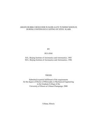
  • 20. 1 CHAPTER 1. INTRODUCTION Continuous casting has been in industrial use for over thirty years and is the predominant way by which steel is produced today in the world. A schematic of part of the typical continuous slab-casting process is depicted in Figure 1.1 [1], showing the tundish, tundish nozzle and mold regions. In a typical slab casting operation, the liquid steel flows from the tundish, through the ceramic tundish nozzle, and exits through bifurcated ports into the liquid pool in the mold. The tundish nozzle consists of the upper tundish nozzle (UTN), the slide-gate plates and the submerged entry nozzle (SEN). Between these two nozzle segments, the flow rate is regulated by moving a” slide gate”, which restricts the opening. Argon bubbles are injected through holes or pores in the nozzle wall to mix into the flowing liquid steel. The nozzle outlet ports are submerged below the surface of the molten steel in the mold to avoid interference with the interface between the steel and the slag layers which float on top. The liquid steel in the mold solidifies against the wall of the water-cooled, copper mold. The solidified steel shell acts as a container for the molten steel as it is continuous withdrawn from the mold at a “casting speed” and grows in thickness as it travels down below the mold. The completely solidified slab is then cut into desired lengths by torches. The quality of the continuous cast steel slab is greatly affected by the flow pattern in the mold, which depends mainly on the flow pattern in the tundish nozzle, specifically the jets from the nozzle port outlets. The flow pattern not only has a great influence on heat transfer to the solidifying shell, but also governs the motion of inclusion particles and surface waves at the meniscus, which affects the internal cleanness and quality of the steel. The tundish nozzle should deliver steel uniformly into the mold while preventing problems such as surface waves, meniscus freezing and crack formation. Impingement of hot liquid metal with high momentum against the
  • 21. 2 solidifying shell can contribute to shell thinning and even costly “breakouts”, where liquid steel bursts from the shell [2]. In addition, the nozzle should be designed to deliver steel with the optimum level of superheat to the meniscus while preventing both detrimental surface turbulence and shell erosion or thinning due to excessive impingement of the hot molten steel jets. In some operations, it is also important for the flow pattern to aid in the flotation of detrimental alumina inclusions into the protective molten slag layer. Plant observations have found that many serious quality problems are directly associated with nozzle operation and the flow pattern in the mold [3]. For example, surface waves and turbulence near the top free surface can entrain some of the slag into the steel flow, causing dangerous large inclusions and surface slivers [4]. The high “standing wave” or large variation in the free surface level at the mold can prevent the liquid mold flux from filling and lubricating the gap between the steel shell and the mold. This can cause cracks in the steel shell due to thermal stresses and mold friction [5]. Nozzle clogging is one of the most disruptive phenomena on the operation of the tundish- mold system. During the casting process, a buildup (clog) containing steel impurities may form and deposit on the nozzle wall. This clog adversely affects product quality by changing the flow pattern which is usually carefully designed, based on no-clogging condition, and by degrading the internal quality of the final product when large chunks of it break off and enter the flow stream. Also, as the buildup progresses, the slide gate opening must be increased to maintain the desired flow rate. Once the slide-gate reaches its maximum position, production must stop and the nozzle must be replaced. Argon injection through the nozzle wall into the steel stream is an efficient and widely employed method to reduce nozzle clogging, even though the real working mechanism is still not fully understood [6]. However, the injected argon bubbles will also affect the flow pattern in the nozzle, and subsequently in the mold. The argon bubbles might attach with small inclusions and
  • 22. 3 become entrapped in the solidifying shell, resulting in “pencil pipe” and blister defects on the surface of the final product [7-10]. Other possible disadvantages of argon injection observed in operation include increased quality defects and nozzle slag line erosion due to the increased meniscus fluctuation [8, 11], exposure of the steel surface and subsequent reoxidation [12], entrapment of the mold power [13]. Large gas injection flow rates might create a boiling action in the mold [14, 15], which can greatly intensify those adverse effects. The boiling action at the mold meniscus was experimentally found [16] related to a flow pattern change inside the tundish nozzle, specifically, the regular “bubbly flow” changes to “annular flow” at high gas flow rate. There is a great incentive to understand and predict the flow through the tundish nozzle since tundish nozzle geometry is one of the few variables that is both very influential on the continuous casting process and relatively inexpensive to change. Designing an effective nozzle requires quantitative knowledge of the relationship between nozzle geometry and other process variables on the flow pattern and the influential characteristics of the jet flow exiting the nozzle. A well-designed nozzle with optimized argon injection implementation should meet the required clogging-resistance capability, prevent the entrapment of those argon bubbles in solidified shell, as well as provide desired flow patterns in both nozzle and mold, which hence help to achieve a high quality cast slab. The effect of gas injection on flow in the nozzle is relatively unstudied, especially through mathematical modeling. Most previous works on modeling fluid flow in the nozzle have focused on single-phase flow [1, 17-19]. A better understanding of fluid flow in the nozzle should consider the effect of gas injection. Argon bubble motion and its effect on flow depends greatly on the size of the bubbles which is determined during the initial stage of gas injection. Bubble size is also an essential parameter for other advanced studies such as argon bubble motion [10],
  • 23. 4 inclusion attachment [10, 20], argon bubble and inclusion entrapment [9], in addition to modeling liquid steel-argon bubble two-phase fluid flow in nozzle and mold [21-23]. This work investigates argon bubble behavior in slide-gate tundish nozzles during continuous casting of steel slabs in three parts. First, water model experiments are performed to study bubble formation behavior in flow conditions approximating those in a slide-gate tundish nozzle of continuous casting process. The effects of liquid velocity, gas injection flow rate, gas injection hole diameter, and gas density on bubble formation behavior such as bubble size, injected gas mode are investigated. An analytical model is developed to predict the bubble size. Secondly, a three-dimensional finite difference model is developed to study the liquid steel- argon bubble two-phase turbulent flow in continuous casting tundish nozzles. Experiments are performed on a 0.4-scale water model to verify the computational model by comparing its prediction with velocity measurements using PIV (Particle Image Velocimetry) technology. A weighted average scheme for the overall outflow is developed to quantify the characteristics of the jets exiting the nozzle ports. Thirdly, the validated model is employed to perform extensive parametric studies to investigate the effects of casting operation conditions and nozzle port design. The interrelated effects of nozzle clogging, argon injection, tundish bath depth, slide gate opening and nozzle bore diameter on the flow rate and pressure in tundish nozzles are quantified using a inverse model, based on interpolation of the numerical simulation results. The results are validated with measurements on operating steel continuous slab-casting machines, and presented for practical conditions. Practical insights to optimize argon injection for various casting conditions are presented. This work is part of a larger project to develop and apply mathematical models to understand and solve problems arising in the continuous casting process.
  • 24. 5 Submerged Entry Nozzle (SEN) Meniscus Copper Mold AAA AAA AAA AAA AAA AAA AAA AAA AAA AAA AAA AAA AAA AAA AAA AAA Slide Gate (flow control) Submergence Depth Liquid Steel Pool Liquid Mold Flux Solidifying Steel Shell AA AA AA AA AA AA AA AA AA AA AA AA AA AA AA AA AA AA Continuous Withdrawal Port Thickness Port Height Port Angle Nozzle Bore Upper Tundish Nozzle (UTN) Molten Steel Jet AAAAA AAA AAA AAAAAAAAA AAAAAAAAA AAAAAAAAA AAAAAAAAA AAAAAAAAA AAAAAAAAA AAAAAAAAA AAAAAAAAA AAAAAAAAA Tundish AAAAAAAA AAAAAAAA AAAAAAAA AAAAAAAA AAAAAAAA AAAAAAAA AAAAAAAA AAAAAAAA AAAAAAAA AAAAAAAAAAA AAAAAAAAAAA Liquid Steel Protective Slag Layer AAAAAAAAAAA Refractory Brick Steel Tundish Wall AAA AAA AAA AAA AAA AAA Solid Mold Powder AA AA AA AA AA AA AA AA A A A AA AA AA Argon Gas Injection Figure 1.1 Schematic of continuous casting tundish, slide-gate nozzle, and mold [1]
  • 25. 6 CHAPTER 2. BUBBLE FORMATION STUDY 2.1 Introduction Argon gas is injected through the walls of the ceramic nozzle into the liquid steel flow to reduce clogging in a slide-gate nozzle. The injected argon bubbles affect the flow pattern in the nozzle, and subsequently in the mold, thereby influencing the steel quality. Thomas et al. [22, 23], modeled the liquid steel-argon bubble two-phase flow in mold, and found that argon bubble size has an important effect that acts in addition to injection rate. Larger bubbles are found to leave the mold faster and, therefore, have less influence on the liquid flow pattern in the mold. Small bubbles travel with the jet further across the mold. Furthermore, small bubbles are more likely penetrate deep into the liquid pool and become entrapped by the solidified shell, causing quality problems, such as “pencil pipe” blister defects [10]. Creech [24] found that smaller bubbles buoyed the jet and encouraged the transition from the classic ”double-roll” flow pattern in the mold to “single-roll” for a given gas fraction. Wang et al. [20] found the optimal bubble size for inclusion removal. Tabata et al. [25] performed water model tests of gas injection into the slide- gate nozzle, and found that large bubbles tended to move to the center of the flow, thus lowering their ability to catch inclusions and to prevent their adherence to the nozzle wall. When argon gas is injected into a slide-gate nozzle through the pores (with typical average diameter of 25~40µm) in the refractory material of the nozzle [6, 7, 26], or via machined or laser cut holes (with typical diameter of 0.2~0.4mm) on the wall [6, 26, 27], the formation of the bubbles is associated with the growth of a liquid-gas interface in an environment subjected to the highly turbulent shearing flow of the liquid steel. The injected gas forms a succession of bubbles which break away from the solid-liquid-gas interface, join the stream of the liquid steel,
  • 26. 7 and thereafter travel as separate entities in the liquid. Or, the injected gas may form a gas sheet along the wall. This possibility is one of several suggested mechanisms for argon injection to deter the clogging in nozzles [6, 11]. We want to know when each happen. 2.2 Literature Review For bubble formation in liquid metals, some experimental works have been reported on gas-stirred vessels in which gas is injected from an upward facing orifice or tube submerged in quiescent liquid. The frequency of bubble formation was measured by using pressure pulse [28, 29], resistance probe [30, 31], or acoustic device [32]. The mean bubble sizes are then derived from the known gas injection flow rate and the measured frequency of bubble formation. Efforts on direct observation of bubble formation in liquid metal were also made by using X-ray cinematography technique [33, 34]. Little work has been reported on bubble formation in flowing liquid metals such as in tundish nozzles. Surface tension and contact angle between the gas, liquid and solid surfaces is also very important to bubble formation. Recently, Wang et al [35] studied the effect of wettability on air bubble formation using water model experiments in which gas was injected through porous refractory into an acrylic tube with flowing water. Wettability as changed by waxing the porous refractory. On the waxed surface, the bubbles tended to coalesce together and form a gas curtain along the wall and then break into many uneven-sized bubbles after travel certain distances. On an un-waxed surface, even-sized bubbles formed and detached from the wall to join the liquid flow. No theoretical modeling work has been reported on bubble formation in metallic systems. On the other hand, extensive bubble formation studies have been done on aqueous systems, both experimentally and theoretically, as reviewed by Kumar and Kuloor (1970) [36],
  • 27. 8 Clift et al. (1978) [37], Tsuge (1986) [38], and Rabiger and Vogelpohl (1986) [39]. Most of those works are about bubble formation in stagnant liquid. The theoretical studies of bubble formation can be divided into two categories: analytical spherical bubble models and discretized non- spherical bubble models. The spherical bubble model assumes the spherical shape of the bubble throughout the bubble growth. The bubble size at detachment is obtained by solving force balance equation and/or bubble motion equation. The forces in equations are evaluated on the whole growing bubble. Two of many significant contributions are the one-stage model by Davidson and Schuler [40] and the two-stage model by Kumar and Kuloor [41]. The spherical bubble models have to use empirical criteria for determining the instant of detachment. In contrast, non-spherical bubble models have been developed [42-45] that are based on a local pressure/force balance at the gas/liquid interface. In these models, the bubble surface is divided into many two-dimensional axis-symmetric elements. For each element, two motion equations, one in the radial direction and the other vertical direction, are solved to give its radial and vertical velocities and then the position of the element. The bubble growth and bubble detachment is determined by calculating the (non-spherical) shape of the bubble during its formation. These models are therefore advantageous because they do not require the assumption of bubble detachment criteria, but not applicable to asymmetric conditions such as with shearing flowing liquid. Direct simulation of bubble formation process using CFD technology was reported by Hong et al. [46] who numerically simulated the formation of a single bubble chain in stagnant liquid by tracking the movement of the gas-liquid interface using the VOF (Volume of Fluid) method [47]. Only a few works [48-50] were reported on bubble formation in flowing liquid condition. In these models, the analytical spherical bubble models of bubble formation in stagnant liquid are modified to accommodate the uniform liquid flow condition by including an additional drag
  • 28. 9 force due to the flowing liquid in the equation of motion. More empirical parameters are introduced in order to match the experimental results, limiting the extension of these models to different conditions. None of these previous models can be directly applied to the current case -- bubble formation in tundish nozzles, in which the gas is horizontally injected through the tiny holes on the inner wall of the nozzle into highly turbulent downward-flowing liquid. 2.3 Water Model Experiments Water model experiments are performed to investigate the bubble formation in flow conditions that incorporate the essential phenomena in tundish nozzle flow. These include high velocity flow of liquid along the wall, which shears the growing bubbles. Direct image visualization and inspection are used to test the effects of liquid velocity, gas injection flow rate, gas injection hole size, and gas composition on the bubble size, shape, frequency, and size distribution. In addition to quantifying these important parameters, the results of these water experiments also serve to validate the theoretical model developed later. 2.3.1 Experimental Apparatus and Procedure Figure 2.1 shows a schematic of the water experimental apparatus. Water flows down from an upper tank that simulates a tundish, through a vertical tube that simulates a tundish nozzle, to a tank at the bottom that simulates a casting mold. The gas (air, helium, or argon) is injected through a plastic tube attached to a hollow needle inserted horizontally into a square 35mm X 35mm Plexiglas tube. Water is made to flow vertically for conditions approximating those in a tundish nozzle. The needle outlet is flush with the nozzle wall to simulate a pierced hole on the inner wall of a nozzle. Three different-sized needles are used to examine the effect of
  • 29. 10 the gas injection orifice diameter (0.2, 0.3, and 0.4 mm). The gas flow controller is adjusted to achieve volumetric gas flow rates of 0.17 ~ 6.0ml/s per orifice. Water flow rate is adjusted by partially blocking the bottom of the nozzle. The average water velocity varies from 0.6m/s to 3.1m/s which corresponds to the pipe Reynolds number of 21,000 ~ 109,000. The water velocity is obtained by measuring the average velocity of the tracing particles that are purposely added to the water. The formation of bubbles is recorded by a high-speed video camera at 4500 frames per second. Each recorded test contains 1000 frame images accounting for 0.22 second measuring time. The head of liquid, defined as the vertical distance between the top surface of the liquid in the upper tank to the needle, is about 500mm and drops less than 20mm during video taping, owing to the short measurement time. The behavior of bubbles exiting the needle is studied by inspecting the video images frame by frame. The frequency (f) of bubble formation is determined by counting the number of the bubbles generated at the exit of the injection needle during the recorded time period. The mean bubble volume (Vb) is easily converted from the known gas injection volumetric flow rate (Qg), via V Q f b g = (2.1) An equivalent average bubble diameter is calculated assuming a spherical bubble, or D Q f b g =       6 1 3 π / (2.2) Bubbles sizes are also measured directly from individual video image in order to validate this procedure and to check the bubble size deviation from its average value. In some testing cases, a second needle is inserted into the nozzle wall 12.5mm downstream the first needle in order to study the interaction between bubbles from the adjacent gas injection sites.
  • 30. 11 2.3.2 Bubble Size in Stagnant Liquid Experiments are first performed with stagnant water where previous measurements and models are available for comparison. This was accomplished simply by closing the opening at the bottom of the tube. Although most previous works are based on bubble formation from an upward facing orifice or nozzle, some authors [32, 36] observed that the bubble sizes from a horizontal orifice were almost the same as those from an upward facing orifice submerged in stagnant liquid. Figure 2.2 shows the measured bubble diameters together with a prediction using Iguchi’s empirical correlation [34]. It can be seen that bubble sizes increase with increasing gas injection flow rate. For the same gas injection rate, a bigger injection orifice produces larger bubbles. At high gas injection rate, larger bubbles emerge from larger diameter orifices. However, orifice size becomes less important at small gas injection rate. The agreement between the experiment data and Iguchi’s correlation prediction is reasonably good. This suggests that Iguchi’s empirical correlation, which is based on relatively large gas injection flow rates and vertical injection, also applies to the horizontal injection and relatively lower gas flow rates of this work. 2.3.3 Bubble Size in Flowing Liquid Experiments are next performed with gas injection into flowing water. The measured mean bubble sizes are plotted in Figure 2.3. Each point in Figure 2.3 represents the mean bubble diameter for one test case with a particular gas injection flow rate, water velocity and gas injection hole size. In addition, the maximum and minimum bubble sizes, obtained by directly measuring the video images for the corresponding case, are shown as “error bars” for each point. Also shown on the figure is the symbol (circle, triangle or square) representing the corresponding mode that will be discussed later in this section.
  • 31. 12 Figure 2.3 shows that the mean bubble size increases with increasing gas flow rate and decreasing water velocity. Comparing Figures 2.2 and 2.3, it can be seen that at the same gas injection rate, the bubble size in flowing liquid is much smaller than in stagnant liquid. This becomes much clearer when the bubble volumes for stagnant liquid and flowing liquid are plotted together, as shown in Figure 2.4. Physically, the smaller bubble size in flowing liquid is natural because the drag force due to the shearing liquid flow acts to shear the bubbles away from the tip of the gas injection hole into the liquid stream before they grow to the mature sizes found in stagnant liquid. The higher the velocity of the shearing liquid flow, the smaller the detached bubbles are. The volumes of the bubbles formed in flowing water, in Figure 2.4, are about 5 ~ 8 times smaller in volume than those in stagnant water. All of the experimental data shown in Figures 2.3 and 2.4 are collected for air. Argon and helium are also used in the experiments to investigate the effect of different gas composition. Figure 2.5 shows that the measured mean bubble diameters for three different gases (air, argon and helium) are about the same. Thus, the gas composition has little influence on bubble sizes. It appears that bubble size is also relatively independent of gas injection hole size. This can be seen when the mean bubble diameters in Figure 2.3 are re-plotted for fixed water velocity, which is illustrated later as comparing with the model predictions in Figure 2.16. This observation is different from that in stagnant liquid, where bubble size is larger for larger gas injection hole. This suggests that the shearing force due to the flowing liquid dominates over other effects related to the hole size such as surface tension force. Figures 2.2-2.5 show that data collected with increasing water velocity generally also has increasing gas flow. This choice of conditions was an unplanned consequence of the greater water flow inducing lower pressure at the orifice, with consequently higher gas flow rate. The higher-speed flowing liquid acts to aspirate more gas into the nozzle. This observation illustrates
  • 32. 13 the important relationship between liquid pressure and gas flow rate that should be considered when investigating real systems. 2.3.4 Bubble Formation Mode It is observed that the initial shape of the bubble exiting the gas injection hole falls into one of four distinct modes, as shown in the representative recorded images of Figure 2.6. Figure 2.7 shows the series of outlines of two typical cases illustrating the formation process of bubbles, corresponding to two different modes, based on tracing the recorded photo series shown in Figure 2.8. For low velocity water flows (less than 1m/s) and small gas injection rates (less than 2ml/s), Mode I is observed. In this mode, uniform-sized spherical bubbles form at the tip of the gas injection hole. They elongate slightly before discretely detaching from the hole and joining the liquid stream, as spherical bubbles again seen in Figure 2.7 top. There is no interaction between the bubbles from the hole of the upper injection needle and the bubbles from the holes of the lower needle if it exists. At the other extreme, Mode IV is observed for high velocity water flows (more than 1.6m/s) and very large gas injection rates (more than 10ml/s). In this mode, each bubble elongates down along the wall, forming a gas curtain, and the curtain merges with the gas from the lower needle, if it exists, to form a long continuous gas curtain. The curtain eventually becomes unstable when its thickness becomes too great and it breaks up into many different size bubbles. Their size ranges from a few that are very large to others that are very tiny. For the range of gas flow of practical interest, this regime is not expected. Mode III is observed for high water flow conditions flows (more than 1.6m/s) and for practical gas injection flow range (less than 6ml/s). Mode III is similar to Mode IV except that
  • 33. 14 there is insufficient gas flow to maintain a continuous gas curtain, so gaps form. Before detaching from the gas injection hole, Figure 2.7 (bottom) documents that the bubbles elongate about 2 times. The bubbles then elongate even more down along the wall and stay attached on the wall for some distance after disconnecting from the gas injection hole. Mode II is a transitional mode between Modes I and III in which the injected gas is elongated along the wall but soon detaches from the wall. If a second gas injection hole exists, the bubbles from the upper hole in Mode II will not coalesce with the bubbles from the lower needle. Bubbles sizes in Mode II are still relatively uniform compared to those in Modes III and IV. In addition to the mean bubble size measured, Figure 2.3 also shows the mode and the bubble size deviation from the mean value, using error bars to represent the size range for each experimental case. All data under 0.9m/s water velocity fall into Mode I and have very small size range, which corresponds to the relatively uniform spherical bubbles detaching near the tip of the hole. This is similar to observation in stagnant liquid. Most data under 1.4m/s water velocity fall into Mode II and have slightly larger size range. For the cases of liquid velocity at 1.9m/s and 2.5m/s, all of the data fall into Mode III and have huge size range, which corresponds to the discontinuous gas curtain broken up into uneven-sized bubbles. The bubble size is as small as 0.5mm in diameter. The continuous gas curtain in Mode IV is observed only at very high gas injection flow rate (Qg > 10 ml/s per hole), which is beyond the practical range of interest, so is not shown in the plots. For Mode III cases, no continuous gas curtain along the wall was observed for those experiments with single needle gas injection. However, those elongated bubbles, after disconnecting from the gas injection hole, still attach and travel along the wall for a certain distance before they finally detach the wall and join the liquid stream, as seen in Figure 2.6 and
  • 34. 15 Figure 2.7 (Bottom). If they meet injected gas from the lower downstream hole before detaching the wall, the two bubble streams coalesce to form larger elongated bubbles. In a real-life tundish nozzle with hundreds of pierced holes or thousands of tiny pores on porous refractory, a continuous gas curtain might be expected on the gas injection section of the inner wall of the nozzle for Mode III. In fact, the argon gas injected into the liquid steel has much bigger tendency to fall into Mode III and to form a gas curtain on the refractory wall due to the much larger surface tension of the liquid steel and the non-wetting behavior of the liquid steel on the refractory material. The experiments also show that no matter what bubble formation mode, the injected gas will eventually detach from the wall, break up into discrete bubbles and join the liquid stream. Therefore, there will be no gas curtain in the tundish nozzle after a certain distance from the gas injection section. It is found that when plotting each experimental data point with the ratio of gas flow rate to mean liquid velocity (Qg/U) as y axis and the gas injection flow rate (Qg) as x axis, the different bubble formation modes fall into separate regions, as shown in Figure 2.9. 2.3.5 Bubble Elongation Measurement Bubble shape is observed to grow and elongate during the formation process. To quantify the effects of the gas flow rate and liquid velocity on bubble elongation, the vertical elongation length (L) is measured at the instant of the detachment of the bubble from its injection hole, as shown in Figure 2.10(A). The measured bubble elongation lengths (L) are plotted in Figure 2.10(B). The effects become clear when plotting the elongation factor, ed, defined as the ratio of the elongation length (L) and the equivalent diameter of the bubble (Db) e L D d b = (2.3)
  • 35. 16 As shown in Figure 2.11(A), the elongation factor mainly depends on liquid velocity, and is relatively independent of the gas injection flow rate. Bubbles elongate slightly more at higher liquid velocity. Figure 2.11(B) illustrates this effect of liquid velocity on the measured average elongation factors. These four data points are well fitted with a simple quadratic function, e = 0.78592+0.70797U - 0.12793U d 2 (2.4) which can be used to estimate the elongation factor at arbitrary liquid velocity rather than those test velocities. 2.3.6 Contact Angle Measurement Contact angles are measured for the purpose of evaluating the surface tension force, which is used later in the model to predict bubble size. The relation between the contact angles and surface tension force are detailed in Appendix A. The static contact angle is defined by the profile adopted by a liquid drop resting in equilibrium on a flat horizontal surface, and was measured to be 50° for the current water experiment. The transverse flowing liquid makes the contact angles no longer uniform along the bubble-solid contact circumference. At the upstream of the bubble, the contact angle increases to θa, defined as the advancing contact angle, and at the downstream of the bubble, the contact angle decreases to θr, defined as the receding contact angle, shown in Figures 2.12 (A). Table 2.1 shows the measured mean contact angles in the water experiments. Generally speaking, the advancing contact angle θa increases with increasing liquid velocity, and the receding contact angle θr decreases with increasing liquid velocity. The effect of gas flow rate is relatively small. Contact angle function, fθ, defined as
  • 36. 17 f o r a θ θ θ θ = − ( ) sin cos cos (2.5) contains all contact angle terms in the surface tension force equation (Equation A.11), In liquid steel-argon system, the surface tension force might have more influence on bubble formation behavior due to significant increase in surface tension coefficient. Unfortunately, except for the static contact angle, which is much larger for steel-argon system (θO =150°) [54] than for water-air system (θO =50°), the advancing and receding contact angles needed in Equation 2.5 are unknown due to lacking experimental data. Estimations on advancing and receding contact angles can be made for elongated argon bubbles in flowing steel, based on the observation in the air-water system. The advancing contact angle θa should be larger than the static contact angle θO (150°) and increases with increasing liquid velocity, but it can not be larger than 180°. The receding contact angle θr should be smaller than the static contact angle and decreases with increasing liquid velocity. It is found from the estimations that the contact angle function fθ might have close values for the steel-argon and water-air systems even though all three contact angles (θO, θa and θr ) are very different between the two systems. For example, if θa =155°(>θO =150°) and θr =124°(>θO =150°) , the contact angle function for the steel-argon system will have the same value (fθ =0.30) as for the water-air system at liquid velocity U=0.9m/s. The contact angle function fθ increases with increasing liquid velocity, as shown in Figure 2.12(B). The four data points are well fitted with a simple quadratic function, f ( ) = -0.06079+0.33109U +0.078773U2 θ U (2.6)
  • 37. 18 Equation 2.6 can be used to estimate the value of the contact angle function at the liquid velocity rather than those tests. 2.4 Mathematical Model to Predict Bubble Size Bubble formation in vertical flowing liquid is very different from the classic bubble formation problem in which the bubble forms at the end of an upward facing orifice or tube submerged in stagnant liquid. In continuous casting process, argon gas is injected into the nozzle horizontally through tiny holes on the inner wall of the nozzle. The injected gas encounters liquid steel flowing downward across its path. The downward shearing liquid flow of interest to nozzle injection is highly turbulent, with a Reynolds number of about 100,000. This turbulent flow exerts a strong shear force on the forming bubble, which greatly affects its formation. Unlike bubble formation in stagnant liquid, in which buoyancy force is the major driving force for bubble detachment, the buoyancy force now acts to resist the premature detachment of the bubble against the drag force of liquid momentum. Thus, previous bubble models can not be directly applied. In developing an analytical model in this work for nozzle injection, the basic ideas from the classic spherical bubble models in stagnant liquid are followed, which are based on balancing the forces acting on the growing bubble and setting a proper bubble detachment criteria. 2.4.1 Forces Acting on a Growing Bubble Correct evaluation of the fundamental forces acting on the growing bubble is essential for an accurate analytical model of bubble formation that can be extrapolated to other systems. A schematic of the fundamental forces acting on a growing bubble is shown in Figure 2.13. The forces of liquid drag, buoyancy, and surface tension are now discussed in turn.
  • 38. 19 Drag force due to flowing liquid FD The drag force exerted by the flowing liquid onto the growing bubble, FD, depends on the liquid velocity. The mean liquid velocity (U) in the nozzle is assumed to be known. Since the growth and detachment of the bubble all occur near the wall and the shearing effect of the flowing liquid creates small bubbles, the steep velocity gradient encountered by the forming bubble are very important. This liquid velocity profile at the wall is needed for accurate evaluation of the drag force. Of the many formulas for velocity profile of a fully developed turbulent flow in a pipe, the most convenient for the current purpose is the seventh root law profile [52] u U y DN =       1 235 2 1 7 . / / (2.7) where y is the distance from the wall, DN is the nozzle diameter, and U is the mean vertical liquid velocity in the nozzle. The average liquid velocity across the growing bubble, u , depends on the instantaneous bubble size and is estimated from u r udy U r D y y r N = = = = ∫ 1 2 1 3173 0 2 1 7 1 7 . / / (2.8) where r is the equivalent horizontal radius of the forming bubble. The drag force acting on the growing bubble, FD, is F C u r D D l = 1 2 2 2 ρ π (2.9) Assuming the bubble Reynolds number, Rebub , is less than 3 105 × , the drag coefficient CD is[37] CD bub bub bub = + + + × − 24 1 0 15 0 42 1 4 25 10 0 687 4 1 16 Re ( . Re ) . / ( . Re ) . . (2.10) where Rebub is defined by
  • 39. 20 Rebub uD = υ (2.11) where D is the equivalent bubble diameter and υ is the kinematic viscosity of the liquid. Buoyancy force FB Buoyancy force acts upward and resists the drag force due to the liquid momentum. F V g D g B b l g l g = − = − ( ) ( ) ρ ρ π ρ ρ 1 6 3 (2.12) Surface tension force FS Surface tension force acts to keep the bubble attached to the wall. The vertical component acts upward to resist drag of the bubble that elongates its shape below the gas injection hole, and is given by [53]. F D Sz O r a = − π σ θ θ θ 4 sin (cos cos ) (2.13) where σ is the surface tension coefficient. Derivation of Equation 2.13 is detailed in Appendix A. The values for θO , θr and θa were measured from the video. Figure 2.14 shows how those three fundamental forces change with the bubble size. Other forces, such as the inertial force due to the rate of change of momentum of the growing bubble, are believed to be negligible. 2.4.2 Two-Stage Model for Bubble Formation in Flowing Liquid A two-stage model is developed to predict the size of the bubbles formed during nozzle injection. The bubble formation is assumed take place in two idealized stages, the expansion stage and the elongation stage, as shown in Figure 2.15.
  • 40. 21 Expansion stage During the expansion stage, the forming bubble expands while holding onto the tip of the gas injection. This stage is assumed to end when the downward forces are first able to balance the upward force. That is, F F F D B Sz = + (2.14) The shape of the bubble during this stage is not considered until at the instant of the force balance when it is assumed to be spherical. Substituting Equations 2.9, 2.12 and 2.13 into Equation 2.14 yields C u r r g r D l l g O r a 1 2 4 3 1 2 2 2 3 ρ π π ρ ρ π σ θ θ θ = − + − ( ) sin (cos cos ) (2.15) In Equation 2.15, u depends on r, which is unknown in advance. Thus, Equation 2.15 is solved for r by trial and error to yield re, which is the equivalent radius of the bubble at the end of the expansion stage. Elongation stage As the bubble continues to grow, the downward force exceeds the upward forces on the bubble. This makes the growing bubble begin to move downward along with the liquid flow. The bubble keeps expanding since it still connects to the gas injection hole, and at the same time it gets elongated due to the shearing effect of the liquid flow. The shape of the bubble in the elongation stage is idealized as ellipsoidal. The connection to the injection hole is assumed through a thin neck, thus the volume in the neck can be neglected. The two horizontal radii of the ellipsoid (rx and ry ) are assumed to be the same to simplify the problem, that is, r r r x y = = (2.16)
  • 41. 22 and the vertical radius of the ellipsoid (rz ) accounts for the effect of the bubble elongation and is related to the equivalent bubble diameter (D) and the elongation factor (e) by r eD z = 1 2 (2.17) The elongation factor should match the measurement defined in Equation 2.3 at the instant of the bubble detachment from its gas injection hole, or r L e D zd d b = = 1 2 1 2 (2.18) where rzd is the vertical radius of the ellipsoid bubble at the instant of the detachment. The instantaneous equivalent diameter (D) of the bubble is related to the instantaneous horizontal radius (r) of the ellipsoid and the instantaneous elongation factor (e) by 1 6 4 3 4 3 1 2 3 2 2 π π π D r r r e D z = =     or D r e = 2 (2.19) The bubble gets more elongated as it grows bigger. The bottom of the ellipsoidal bubble is assumed to travel along with the liquid at the average velocity u , defined in Equation 2.8. Criterion to end this final stage of bubble growth is the detachment of the bubble from the gas injection hole when the bubble elongates to the measured elongation at detachment. This corresponds to the time when the vertical distance traveled by the fluid, from point A to B, equals the critical length at the instant of bubble detachment, as shown in Figure 2.15(B). udt e D d r t t d b e e d ∫ = + − 2 (2.20) Substituting Equation 2.19 into Equation 2.20 yields udt r e d r t t d d e e d ∫ = + − 2 2 3 2 / (2.21)
  • 42. 23 where te and td are the bubble growing times at the end of the expansion stage and the instant of bubble detachment respectively. rd is the horizontal radius at the detachment. The bubble growing time (t) is related to the instantaneous horizontal radius of the growing ellipsoidal bubble (r) by volume conservation, which assumes that pressure and temperature are sufficient uniform to avoid compressibility effects. Q t D g = 1 6 3 π (2.22) Substituting Equation 2.19 into Equation 2.22 yields t Q r e g = 4 3 3 3 2 π / (2.23) Also knowing e at r r e at r r e d d = = =      1 (2.24) the elongation factor at can be approximated by a linear function e ar b at r r r e d = + < < (2.25) The values of the constant a and b can be derived by satisfying the conditions in Equation 2.24: a e r r d d e = − − 1 (2.26) b r e r r r d d e d e = − − (2.27) From Equation 2.23 and Equation 2.25, dt d Q r e Q r ar b ar ar b dr g g =       = + ( ) + + ( )       4 3 4 2 3 3 2 2 3 2 3 1 2 π π / / / (2.28) Substituting Equation 2.8 and Equation 2.28 into Equation 2.21 yields 5 2692 2 1 7 2 3 1 2 1 7 3 2 1 7 . / / πU Q D r ar b ar ar b dr g N r r e d + ( ) + + ( )       ∫ = + − 2 2 3 2 r e d r d d e / (2.29)
  • 43. 24 It should be noted that there are no adjustable parameters in this model. The elongation factor at the instant of the bubble detachment (ed) and the contact angle function (fθ) depend on the mean liquid velocity (U), and are obtained from the experimental measurements, shown in Figures 2.11 and 2.12. To extend the model for the arbitrary liquid velocity beyond the test, the extrapolated quadratic function, Equations 2.4 and 2.6, are used in the model. Equation 2.29 are solved iteratively by trial and error for the horizontal radius of the ellipsoidal bubble at the instant of detachment from the gas injection hole, rd, which is the only unknown in this equation, using a program written in MATLAB detailed in Appendix B. The equivalent bubble diameter is then converted from Equation 2.19 to D r e b d d = 2 (2.30) 2.4.3 Comparing with Measurements The bubble diameters predicted by the two-stage model are shown in Figure 2.16, along with the measured mean bubble diameters. The physical properties of the fluids and operating conditions used in calculation are summarized in Table 2.2 Figure 2.16 shows that the match between the model prediction and the experimental data is reasonably good, although the predicted slopes (dD/dQg) appear to be slightly smaller than experimental results. This means the model may slightly over-predict the bubble size for the low gas injection flow rates and under-predict the bubble size for the high gas flow rates. Figure 2.16 shows the same trends of the effects of the liquid velocity and gas flow rate on bubble sizes as observed during the experiments, that is, the mean bubble size increases with increasing gas injection flow rate and decreasing shearing liquid velocity. Figure 2.16 shows that the gas injection hole size rarely affects the bubble size at high liquid velocity (U≥1.4m/s). This agrees with the water experiments that could hardly tell the
  • 44. 25 difference for the data measured from different hole sizes. However, at relatively low liquid velocity, as shown in the plot for U=0.9m/s in Figure 2.16, the influence of the hole size becomes slightly obvious, and the larger gas injection hole generates slightly larger bubbles. This match the trends observed in the experiments for the stagnant liquid condition, which showed an important effect of gas injection hole size on bubble size. The two-stage model also predicts a negligible effect of the gas density that again matches the experimental measurements. The gas density appears only in the buoyancy term in the force balance Equation 2.15 in the form of (ρl-ρg), which is easy to see being negligible compared with the liquid velocity. There still exist some discrepancies between the predictions and measurements, as shown in Figure 2.15. Random errors found in the experiments are likely one of the main sources. The experiments were performed at highly turbulent flow conditions (experimental Reynolds numbers range from 21,000 to 109,000), which is transient and random in nature. The recorded 1000 frame images for each case are for the period of only 0.22 second, which is not long enough to make a good time average. 2.5. Argon Bubble Sizes in Liquid Steel 2.5.1 Difference between Steel-Argon and Water-Air Systems In order to use the two-stage model developed above and validated for a water-air system to predict the bubble size in the liquid steel-argon system in tundish nozzles, it is important to understand the difference between the two systems. As seen in Table 2.2, there is big difference in physical properties between the steel-argon system and water-air system. For example, the surface tension coefficient for the liquid steel-argon system is more than 16 times of that of the
  • 45. 26 water-air system. The density of the liquid steel is 7 times of the water density. The effects of these physical properties on bubble formation are incorporated in the two–stage model. Except for the static contact angle, which is much larger for steel-argon system than for water-air system [54], the advancing and receding contact angles needed in Equation 2.15 are unknown for the liquid steel-argon system due to lacking experimental data. As discussed in Section 2.3.6, the contact angle function fθ (=sinθο(cosθr-cosθa)) from the water experiment might be close to the steel-argon system, thus adopted in calculation, as shown in Table 2.2. Measurements [34] and calculation (Appendix C) show that gas injected through the “hot” ceramic wall heats up to 99% of the liquid steel temperature even before it hits the liquid steel. Thus, the argon gas injection flow rate used in the model is the “hot” argon flow rate. 2.5.2 Predicting Bubble Size in Tundish Nozzles The two-stage model is used to predict argon bubble sizes in liquid steel in a typical tundish nozzle with 78mm bore diameter. Air bubble sizes in water is also predicted for the same conditions, as shown in the rightmost column of Table 2.2, for direct comparison. The predictions are presented in Figure 2.17, showing the predicted bubble diameter vs. gas injection flow rate under different liquid velocities. The argon bubble size increases with increasing gas flow rate and decreasing liquid velocity, same trends as the air bubble size in water. In general, argon bubbles generated in liquid steel are predicted to be larger than air bubbles in water. The difference becomes more significant at lower liquid velocity and smaller gas flow rate. For the practical interested range of the liquid velocity in tundish nozzles (0.7~1.2m/s), the difference in bubble size between the two systems is sometimes significant. For example, a typical tundish nozzle with 140 holes and 7 SLPM argon injection on UTN has 3.5 ml/s hot argon flow rate for each hole. At the mean liquid velocity of 0.7m/s, the diameters of the argon bubbles in liquid
  • 46. 27 steel are about 1.5 times of those air bubbles in water, and the corresponding volumes of the argon bubbles are 3.4 times of those of air bubbles. The reason for larger bubbles predicted in the steel-argon system is mainly due to the great difference in liquid density and surface tension coefficient in steel-argon system. This make the drag force and surface tension force acting on the forming argon bubbles in liquid steel much larger than those forces on the forming air bubble in water, under the same flow conditions. Since the increase in surface tension force is more than two times of the increase in drag force, the force balance of Equation 2.15 will be satisfied at a larger bubble size re at the end of the expansion stage when compared to the water-air system. At very high liquid velocity, the drag force due to the flowing liquid become so dominant that increase in surface tension force becomes less important to the bubble formation behavior and thus the difference in bubble sizes become smaller for the two systems. Figure 2.18 plots the predicted bubble size for varying liquid velocity at a few fixed gas flow rates for both systems. The two-stage model could not handle the very low liquid velocity conditions. The program in Appendix B blowups at U<0.5m/s for water-air system and U<0.7m/s for steel-argon system. Physically, this is because that at very low velocity downward liquid flow, the downward drag force might not be able to balance the upward buoyancy force and surface tension force. The bubble might go upward. The model need modification to deal with the upward moving situation, in which the advancing contact angle and receding contact angle switch positions and the surface tension force change its direction. The steel-argon system blowups at higher liquid velocity due to its much higher surface tension than water-air system. Since the ratio of the liquid and gas density for steel-argon system (ρl /ρg =104 ) is one order higher than for water-air system (ρl /ρg =103 ), gas density should have no effect on argon
  • 47. 28 bubble size in liquid steel for the same reason as in water-air system. The effect of the gas injection hole on argon bubble size is similar like air bubbles in water, although it is not plotted here. 2.5.3 Discussion The elongation factor and contact angle function fθ obtained from the water model experiment, are directly employed for the tundish nozzle conditions due to lacking the experimental data for liquid steel-argon system. The mean argon bubble size in liquid steel predicted with the two-stage model is conservative or under-predicted due to the difference in wettability. The non-wetting property of liquid metal on ceramics nozzle wall, in contrast to the aqueous wetting system, makes the forming bubble tend to spread more over the wall, which has been observed by other authors [32, 34, 35]. The spreading bubble might have a larger elongation factor in this system. This will likely result in an under-predicted bubble size. On the other hand, the tendency for argon bubbles to spread over the ceramics nozzle wall makes the bubble formation mode fall into Mode II or III region at lower liquid velocity than water-air system. Therefore, the argon bubbles should have larger tendency to have uneven sizes when detaching from the wall. The two-stage model predicts only the average bubble size, but not other important gas bubble behavior such as bubble formation mode, bubble shape, bubble size deviation, bubble coalescence and break-up. Direct numerical simulation of bubble formation process by tracking the movement of the gas-liquid interface is a potential method to overcome these limitations. Simulation of a single bubble chain in stagnant liquid using the VOF method has been reported [46] to agree well with the experimental results in a real time sequence. However, numerical
  • 48. 29 simulation of argon bubble formation in a tundish nozzle condition is still a challenge, likely due to the complex effects of turbulence, boundary layer, surface tension and wettability. 2.6 Summary Water experiments are performed to study bubble formation from a horizontal oriented hole facing a shearing downward turbulent liquid flow, approximating conditions in a tundish nozzle. The effects of various parameters such as liquid velocity, gas injection flow rate, hole diameter, and gas density on bubble formation behavior such as bubble size, injected gas mode have been investigated. An analytical two-stage model based on force balance and bubble formation sequence is developed to predict the bubble size at detachment from it gas injection hole. Model predictions show good agreement with the measurements. The model is then used to predict the size of the argon bubbles generated in liquid steel of a tundish nozzle. Specific findings include: • The mean bubble size increases with increasing gas injection flow rate. • The mean bubble size increases with decreasing shearing liquid velocity. • The mean bubble size in flowing liquid is significantly smaller than in stagnant liquid. • The mean bubble size is relatively independent of gas injection hole size, especially at high liquid velocity • The gas composition has little influence on bubble size. • Bubble formation falls into one of the four different modes, depending primarily on the velocity of the flowing liquid and secondarily on the gas flow rate. • In Mode I (low liquid speed and small gas flow rate), uniform-sized bubbles form and detach from the wall. In Mode III (high liquid speed), the injected gas elongates down along the wall and breaks into uneven sized bubbles. Mode II is intermediate between
  • 49. 30 Mode I and Mode III. In Mode IV (high liquid speed and high gas flow rate), the gas elongates a long distance down the nozzle walls, forming a sheet before breaking up. • Compared to water-air system, argon bubbles in liquid steel should tend to spread more over the ceramic nozzle wall in liquid steel and fall into Mode II or III region. Thus, the argon bubbles likely have a larger tendency to have non-uniform sizes when detaching from the wall. • Argon bubbles generated in liquid steel should be larger than air bubbles in water for the same flow conditions. The difference should become more significant at lower liquid velocity and smaller gas injection flow rate.
  • 50. 31 Table 2.1 Average contact angles measured in the water experiments Average liquid velocity (m/s) Static contact angle θO (°) Advancing contact angle θa (°) Receding contact angle θr (°) Contact angle function fθ =sinθΟ(cosθr-cosθa) 0.9 50 64 35 0.30 1.4 50 82 29 0.56 1.9 50 101 22 0.85 2.5 50 134 27 1.26 Table 2.2 Physical properties and operating conditions used in the two-stage model Parameters Symbol Unit Water-Air System for matching measurements Steel-Argon System Water-Air System for comparison Liquid density ρl Kg m / 3 water: 1000 liquid steel: 7021 water: 1000 Gas density ρg Kg m / 3 air: 1.29 hot argon: 0.27 air: 1.29 Liquid viscosity µl kg/(ms) water: 0.001 liquid steel: 0.0056 water: 0.001 Gas viscosity µg kg/(ms) air: 1.7E-5 hot argon: 7.42E-5 air: 1.7E-5 Surface tension coefficient σ N/m 0.073 1.192 0.073 Gas injection flow rate/pore Qg ml/s air: 0.1 ~ 6 ml/s hot argon: 0.1 ~ 6 ml/s air: 0.1 ~ 6 ml/s Nozzle diameter Dn mm 35 78 78 Diameter of gas injection hole d mm 0.2, 0.3, 0.4 0.2, 0.3, 0.4 0.2, 0.3, 0.4 Average velocity of the liquid U m/s 0.9, 1.4, 1.9, 2.5 0.7, 0.9, 1.4 1.9, 2.5 0.7, 0.9, 1.4 1.9, 2.5 Elongation factor at detachment ed 1.32, 1.53, 1.67, 1.76 ed (U) = 0.78592 + 0.70797U - 0.12793U2 Contact angle function sinθο(cosθr-cosθa) fθ 0.30, 0.56 0.85, 1.26 fθ(U)= - 0.06079 + 0.33109U + 0.078773U2
  • 52. 33 0 1 2 3 4 5 6 0 1 2 3 4 5 Iguchi (d=0.2) Iguchi (d=0.3) Iguchi (d=0.4) measured (d=0.2) measured (d=0.3) measured (d=0.4) Mean bubble diameter (mm) Gas injection flow rate (ml/s) d: Gas injection hole diameter (mm) Figure 2.2 Measured air bubble sizes in stagnant water and prediction from Iguchi's empirical correlation [34]
  • 53. 34 0 0.5 1 1.5 2 2.5 3 3.5 0 1 2 3 4 5 Mode I Mode II Mode III Bubble diameter (mm) Gas injection flow rate (ml/s) U=0.9m/s U=1.4m/s U=1.9m/s U=2.5m/s Gas inj. hole diameter d=0.4mm 0 0.5 1 1.5 2 2.5 3 3.5 0 1 2 3 4 5 Mode I Mode II Mode III U=0.9m/s U=1.4m/s U=1.9m/s U=2.5m/s Gas injection flow rate (ml/s) Bubble diameter (mm) Gas inj. hole diameter d=0.3mm 0 0.5 1 1.5 2 2.5 3 3.5 0 0.5 1 1.5 2 2.5 3 3.5 Mode I Mode II Mode III U=0.9m/s U=1.4m/s U=1.9m/s U=2.5m/s Gas injection hole diameter d=0.2mm Bubble diameter (mm) Gas injection flow rate (ml/s) Figure 2.3 Measured air bubble sizes under different gas injection flow rate and water velocity and the effect of the modes to bubble size deviation to their mean values
  • 54. 35 0 0.01 0.02 0.03 0.04 0 0.2 0.4 0.6 0.8 1 1.2 1.4 Flowing liquid (d=0.2) Flowing liquid (d=0.3) Flowing liquid (d=0.4) Stagnant liquid (d=0.2) Stagnant liquid (d=0.3) Stagnant liquid (d=0.4) Mean bubble volume (ml) Gas injection flow rate (ml/s) Mean liquid velocity: 0.9m/s Gas inj. hole diameter: d (mm) Figure 2.4 Comparison of air bubble volumes in stagnant liquid and flowing liquid
  • 55. 36 0 0.5 1 1.5 2 2.5 3 0 0.5 1 1.5 2 2.5 3 3.5 U=0.9, Air U=0.9, He U=0.9, Ar U=1.4, Air U=1.4, He U=1.4, Ar U=1.9, Air U=1.9, He U=1.9, Ar U=2.5, Air U=2.5, He U=2.5, Ar U=0.9 U=1.4 U=1.9 U=2.5 Gas injection hole diameter d=0.2mm Mean liquid velocity :U (m/s) Gas injection flow rate (ml/s) Mean bubble diameter (mm) Figure 2.5 Effect of gas composition, gas flow rate and liquid velocity on bubble size
  • 56. 37 Mode I Mode II Mode III Mode IV Figure 2.6 Photograph of the four bubble formation modes observed in the experiments
  • 57. 38 AA AA AA AA AA A A A A A AA AA AA AA AA A A A A A AA AA AA AA AA AA AA AA AA AA A A A A A AA AA AA AA AA AA AA AA AA AA A A A A A AA AA AA AA A A A A AA AA AA AA A A A A A AA AA AA AA AA AA AA AA AA AA A A A A A AA AA AA AA AA A A A A A AA AA AA AA AA Mode I (U=0.9m/s, QG=0.5ml/s, d=0.4mm), Bubble frequency f=293s-1 Equivalent bubble diameter: measured: 1.51mm, predicted: 1.53mm Mode III (U=1.9m/s, QG=1.86ml/s, d=0.3mm), Bubble frequency f=444s-1 Equivalent bubble diameter: measured: 2.0mm, predicted:1.95mm t=0 t=0.44ms t=0.89ms t=1.33ms t=1.78mm t=2.22ms t=2.67ms t=3.11ms t=3.56ms t=4.00ms t=0 t=0.44ms t=0.89ms t=1.33ms t=1.78mm t=2.22ms t=2.67ms t=3.11ms t=3.56ms t=4.00ms Figure 2.7 Traced bubble formation process for Mode I and Mode III
  • 58. 39 t=0 t=0.44ms t=0.89ms t=1.33ms t=1.78mm t=2.22ms t=2.67ms t=3.11ms t=3.56ms t=4.00ms t=0 t=0.44ms t=0.89ms t=1.33ms t=1.78mm t=2.22ms t=2.67ms t=3.11ms t=3.56ms t=4.00ms Mode I (U=0.9m/s, QG=0.5ml/s, d=0.4mm), Bubble frequency f=293s-1 Equivalent bubble diameter: measured: 1.51mm, predicted: 1.53mm Mode III (U=1.9m/s, QG=1.86ml/s, d=0.3mm), Bubble frequency f=444s-1 Equivalent bubble diameter: measured: 2.0mm, predicted:1.95mm Figure 2.8 Photo series showing the traced bubble formation process for Mode I and Mode III
  • 59. 40 0 0.5 1 1.5 2 2.5 0 1 2 3 4 5 Mode I Mode II Mode III Gas flow rate (ml/s) / Liquid velocity (m/s) Gas injection flow rate (ml/s) Figure 2.9 Bubble formation modes and their relation with liquid velocity and gas injection flow rate
  • 60. 41 AA AA AA AA AA AA AA L Nozzle wall Q g Liquid flow U ed =L/Db 0 1 2 3 4 5 6 0 1 2 3 4 5 U=2.5m/s U=1.9m/s U=1.4m/s U=0.9m/s Measured elongation length (mm) Gas injection flow rate (ml/s) Gas injection hole diameter: d=0.4mm Mean liquid velocity: U (A) Schematic of the measurement (B) Measured elongations (L) Figure 2.10 Bubble elongation length at instant of bubble detachment from the gas injection hole
  • 61. 42 0 0.5 1 1.5 2 0 1 2 3 4 5 U=2.5m/s U=1.9m/s U=1.4m/s U=0.9m/s Measured elongation factor at detachment e d (=L/D) Gas injection flow rate (ml/s) Gas injection hole diameter: d=0.4mm Mean liquid velocity: U Ave. ed =1.76 Ave. e d =1.67 Ave. ed =1.53 Ave. ed =1.32 (A) 0 0.5 1 1.5 2 0.5 1 1.5 2 2.5 Measured ave. Curve-fitting Elongation factor at detachment e d Mean liquid velocity U (m/s) Curve-fitting model: ed = 0.78592+0.70797*U-0.12793*U2 Gas injection hole diameter: d=0.4mm (B) Figure 2.11 Measured average elongation factor at bubble detachment (A) and its extrapolation (B)
  • 62. 43 θa Liquid flow θr θa θr Liquid flow Water-air system Steel-argon system (A) 0 0.5 1 1.5 0.5 1 1.5 2 2.5 Measured ave. Curve fitting Curve-fitting model: f 0 (U)=-0.06079+0.33109*U+0.078773*U2 Contact angle function Mean liquid velocity U (m/s) (B) Figure 2.12 Advancing and receding contact angles (A) and contact angle function extrapolation (B)
  • 63. 44 Liquid Velocity Profile u=u(y) y 0 z Gas injection Liquid Flow Mean Velocity U FB FSZ FS FQ FSY FD Qg Nozzle wall d θr θa Figure 2.13 Schematic of forces acting on a growing bubble and liquid velocity profile near wall region in the expansion stage
  • 64. 45 10-8 10 -7 10-6 10-5 10-4 10-3 10-2 0 0.5 1 1.5 2 2.5 Drag force F D Buoyancy force F B Surface tension force FSZ Forces acting on the growing bubble (N) Radius of a growing bubble (mm) Mean liquid velocity U=0.9m/s Gas injection hole dia. d=0.4mm Figure 2.14 Evolution of vertical forces acting on a growing bubble with increasing bubble size
  • 65. 46 Liquid flow U Qg Gas injection Liquid flow U Qg Gas injection 2r d e d 3/2 +d /2 -r e L=D b e d =2 r d e d 3/2 Nozzle wall Nozzle wall 2rd d/2 u(r) 2re u(r) A B z y 2re r e (A) Expansion stage (B) Elongation stage Figure 2.15 Idealized sequence of bubble formation in the two stage model
  • 66. 47 0 0.5 1 1.5 2 2.5 0 0.2 0.4 0.6 0.8 1 1.2 1.4 d=0.4mm,measured d=0.3mm,measured d=0.2mm,measured d=0.4mm,predicted d=0.3mm,predicted d=0.2mm,predicted Mean bubble diameter (mm) Gas injection flow rate (ml/s) Mean liquid velocity U=0.9m/s d: Gas injection hole diameter 0 0.5 1 1.5 2 2.5 3 0 0.5 1 1.5 2 2.5 d=0.4mm,measured d=0.3mm,measured d=0.2mm,measured d=0.4mm,predicted d=0.3mm,predicted d=0.2mm,predicted Mean bubble diameter (mm) Gas injection flow rate (ml/s) Mean liquid velocity: 1.4m/s d: Gas inj. hole diameter 0 0.5 1 1.5 2 2.5 3 0 0.5 1 1.5 2 2.5 3 3.5 d=0.4mm, measured d=0.3mm, measured d=0.2mm, measured d=0.4mm, predicted d=0.3mm, predicted d=0.2mm, predicted Mean bubble diameter (mm) Gas injection flow rate (ml/s) Mean liquid velocity: 1.9m/s d: Gas injection hole diameter 0 0.5 1 1.5 2 2.5 3 3.5 0 1 2 3 4 5 d=0.4mm, measured d=0.3mm, measured d=0.2mm, measured d=0.4mm, predicted d=0.3mm, predicted d=0.2mm, predicted Mean bubble diameter (mm) Gas injection flow rate (ml/s) Mean liquid velocity: 2.5m/s d: Gas injection hole diameter Figure 2.16 Comparison of the predicted air bubble sizes in water with measurements
  • 67. 48 0 1 2 3 4 5 6 7 0 1 2 3 4 5 6 Steel-argon system Water-air system Mean bubble diameter (mm) Gas injection flow rate (ml/s) Mean liquid velocity U=0.7m/s Gas injection hole diameter d=0.3mm 0 1 2 3 4 5 6 7 0 1 2 3 4 5 6 Fe-Ar@U=0.9 Fe-Ar@U=1.4 W-Air@U=0.9 W-Air@U=1.4 Mean bubble diameter (mm) Gas injection flow rate (ml/s) Gas injection hole diameter d=0.3mm Fe-Ar: Liquidsteel-Argon system W-Air: Water-Air system U: Mean liquid velocity (m/s) 0 1 2 3 4 5 6 7 0 1 2 3 4 5 6 Fe-Ar@U=1.9 Fe-Ar@U=2.5 W-Air@U=1.9 W-Air@U=2.5 Mean bubble diameter (mm) Gas injection flow rate (ml/s) Gas injection hole diameter d=0.3mm Fe-Ar: Liquidsteel-Argon system W-Air: Water-Air system U: Mean liquid velocity (m/s) Figure 2.17 Comparison of the predicted argon bubble diameters in liquid steel with air bubble diameters in water
  • 68. 49 0 1 2 3 4 5 6 0.5 1 1.5 2 2.5 Fe-Ar@Qg=5 Fe-Ar@Qg=3 Fe-Ar@Qg=1 W-Air@Qg=5 W-Air@Qg=3 W-Air@Qg=1 Mean liquid velocity U (m/s) Fe-Ar: Steel-Argon system W-Air: Water-Air system Qg: Gas injection rate (ml/s) Gas injection hole diameter d=0.3mm Mean bubble diameter (mm) Figure 2.18 Effect of the mean liquid velocity and gas flow rate on argon bubble in liquid steel and air bubble in water
  • 69. 50 CHAPTER 3. TWO-PHASE FLOW IN SLIDE-GATE NOZZLES 3.1 Previous Work Previous works on modeling flow in nozzles have focused on single-phase flow. Hershey, Najjar and Thomas [1, 55] assessed the accuracy of the two- and three-dimensional finite-element simulations of the single-phase flow in a bifurcated submerged entry nozzle (SEN) through comparison with velocity measurements and water modeling observations. They demonstrated the reasonable accuracy of separating the nozzle and mold calculations and using 2-D simulations for some symmetrical flows. Their work was later extended [17] to perform an extensive parametric study of single-phase symmetrical flow in the nozzle. Wang [18] employed a 3-D finite-element single-phase model of a complete tundish nozzle (including the upper tundish nozzle, the slide-gate, and the SEN) to confirm the asymmetrical flow caused by the slide gate. Yao [19] used a finite-volume method to model flow through the SEN and the mold together. Experimental works have reported the importance of two-phase flow in nozzles when argon injected. Tsai [56] observed the partial vacuum pressure at the upper portion of SEN in the water experiments, and found that proper argon injection might avoid the vacuum pressure and hence reduce the air aspiration. Heaslip et al. [57] performed water model experiments to investigate the use of injected gas to carry alloying elements into the liquid. Burty et al. [16] observed a flow pattern transition from dispersed bubbly flow to “annular” flow where gas and liquid separates. A criterion for this transition was developed based on water model experiments through stopper-rod nozzles that depends on both gas flow rate and liquid flow. Sjöström et al. [58] performed an experimental study of argon injection and the aspiration of air into a stopper
  • 70. 51 rod using liquid steel, and found that air aspiration could be reduced by increasing the argon flow rate or pressurizing the stopper. Little work has been reported on the mathematical modeling of the two-phase flow in nozzles, although some studies have been published on the two-phase flow in the ladle [59, 60] and mold [21, 22]. Several different methods have been developed to simulate multiphase flow in continuous casting process. Thomas et al. [10] tracked the trajectories of individual bubbles through the liquid steel in a mold using a Lagrangian approach for particle transport. The effect of the argon bubbles on the steel flow pattern was neglected, so, the results only apply to low argon flow rates. Bessho et al. [21] and Thomas and Huang [22] modeled the gas-liquid flow in the mold by solving the 3-D, incompressible, steady-state, mass and momentum conservation equations for the liquid phase. The buoyancy effect of the gas bubbles was taken into account by adding an extra force term in the liquid momentum equation in the vertical direction. Bubble dispersion in the gas–liquid mixture due to turbulent transport and diffusion was modeled by solving a transport equation for the continuum gas volume fraction. To simplify the problem, no momentum equation was solved for the gas phase. Instead, the bubbles were assumed to reach their steady-state terminal velocity immediately upon entering the domain. An enhancement on this procedure is the Eulerian “homogeneous model” [61, 62] which still solves only a single set of transport equations, but adopts mixture properties where the density and viscosity are proportional to the volume fraction of the phases. The volume fractions are function of space and sum to one on each cell. Another form of multiphase flow models [47] solves the transport equations only for liquid phase. The gas-liquid interface is defined by a transport equation and diffusion across the interface is prevented. The volume fractions are equal to one or zero everywhere except the interface. This method is usually used for free surface flows and stratified flows, tracking
  • 71. 52 movement of gas-liquid interface such as the case of non-dispersed flow or tracking individual bubble formation [46], and might be suitable for modeling annual flow in nozzles. Creech [24] investigated the turbulent flow of liquid steel and argon bubble in the mold using the multi-fluid Eulerian multiphase model, in which one velocity field for the liquid steel and a separate velocity field for the gas phase are solved. The momentum equation for each phase is affected by the other phase through inter-phase drag terms. This approach is adopted in current work. 3.2 Model Formulation The nozzle controls the flow pattern developed in the mold by governing the speed, direction, swirl and other characteristics of the liquid jet entering the mold. The computational domain for simulating flow through a typical slide-gate nozzle is shown in Figure 3.1 with its boundary conditions. The top of the nozzle is attached to the bottom of a tundish and the outlet ports of the nozzle exit into the continuous casting mold. 3.2.1 Governing Equations Flow in this nozzle is inherently three-dimensional, two-phase and highly turbulent. The Reynolds number, based on the nozzle bore diameter (DN), is typically of the order of 105. A multi-fluid Eulerian multiphase model is used to simulate the time-average flow of argon bubbles in liquid steel. Each phase has its own set of continuity and momentum equations. Coupling is achieved through an empirical inter-phase drag between liquid steel and argon bubbles. The governing equations of mass and momentum balance for the liquid phase are: