1. Nathanael Melia | Ed Hawkins | Keith Haines
Department of Meteorology
Predicting the Opening of Arctic Sea Routes
A53C-0389: Improved Arctic Sea Ice Thickness Projections Using Bias Corrected CMIP5 Simulations
Method development
SIT is a particularly challenging variable and using traditional bias
correction techniques results in unwanted behaviour (Fig. 3). In
refining our methods we created the Mean And VaRIance
Correction (MAVRIC).
MAVRIC validation
We test MAVRIC using a data denial method where using the
CSIRO-Mk3.6.0 GCM (CSIRO) we calibrate CSIRO with MAVRIC
using the first 20 years of PIOMAS observations to test how
MAVRIC predicts the following 15 years of observations. It is clear
from the validation bean plots (Fig. 4 right) that the distribution
of CSIRO post MAVRIC matches PIOMAS closer than raw CSIRO.
Introduction
Arctic sea ice thickness
• To represent observations of SIT we use the coupled ice-ocean
model PIOMAS (Fig. 1) which is forced with reanalysis.
• Global climate models (GCMs) all show distinct spatial and
temporal biases. This makes their use for impact-based climate
change studies problematic.
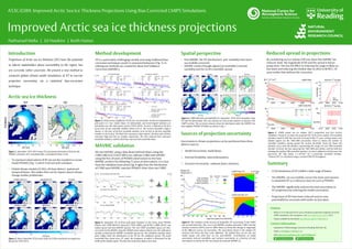
Spatial perspective
Sources of projection uncertainty
Uncertainty in climate projections can be partitioned into three
distinct sources .
1. Model Uncertainty: model biases.
2. Internal Variability: natural fluctuations.
3. Scenario Uncertainty : unknown future emissions.
Improved Arctic sea ice thickness projections
• In
• Summary
Figure 1. September 1979–2014 mean SIT and standard deviation (SD) from the
PIOMAS reanalysis. SD is calculated after removing the linear trend.
Projections of Arctic sea ice thickness (SIT) have the potential
to inform stakeholders about accessibility to the region, but
are currently rather uncertain. We present a new method to
constrain global climate model simulations of SIT to narrow
projection uncertainty via a statistical bias-correction
technique.
• Post MAVRIC the SIT distributions and variability have been
successfully corrected.
• MAVRIC retains (though adjusts) an ensemble’s internal
variability and the GCM’s ensemble spread.
Figure 2. Mean September SIT for each of the six GCMs considered, averaged over
the period 1979–2014.
Figure 3. Performance of different SIT BCs for one particular month at a hypothetical
grid point in a ‘toy’ model. Mean, SD (detrended), and trend legend statistics are
calculated over the observation period (1979–2014). ‘Ice-free’ is defined as the first
occurrence of any ensemble member below 0.15 m. The ice-free ensemble range is
shown; i.e. the year of the first ensemble member to be ice-free to the last ensemble
member to be ice-free. The black line represents ‘observations’; the blue and red lines
represent high and low ice models respectively. The thin coloured lines represent
ensemble members, and the thick lines represent the ensemble mean.
Figure 4. September SIT at three grid point locations in the Arctic, from PIOMAS
(black) and CSIRO-Mk3.6.0 historical (1979–2005) and RCP8.5 (2006–2014) raw
output (grey) and post-MAVRIC (green). The raw CSIRO ensembles (grey) are bias-
corrected via the MAVRIC using the PIOMAS observations (black) over the calibration
window, producing the MAVRIC ensembles (green) for the validation window. Bean
plots (right) show the distribution of the SIT for the validation period. The small
horizontal lines show every SIT value, the frequency of which is illustrated by the
width of the shaded region. The thick horizontal line depicts the mean.
Figure 5. CSIRO-Mk3.6.0 and HadGEM2-ES, September 1979–2014 ensemble mean
SIT and SD (detrended). The raw columns are the model solutions as found in the
CMIP5 archive. The corrected columns show the distribution after the MAVRIC has
been applied. PIOMAS SIT fields are shown in Fig. 1.
Figure 6. The evolution of the sources of September SIT uncertainty in the CMIP5
sub-set with lead time. Year zero is the MAVRIC window mid-point (1997) and the
emission scenarios (RCPs) start in 2006. Panel (a) shows the change in magnitude
of the different sources of uncertainty. The uncertainty shown is the median SIT
variance and hence the lines scale additively. The dashed lines are for the raw
model output and solid lines are for post-MAVRIC. Contributions of model
uncertainty, internal variability, and scenario uncertainty as a fraction of total
uncertainty are shown for the raw output (b) and post-MAVRIC (c).
Citation
• Melia, N. et al: Improved Arctic sea ice thickness projections using bias corrected
CMIP5 simulations, The Cryosphere., doi: 10.5194/tc-9-2237-2015, 2015.
• Dataset available for download: http://dx.doi.org/10.17864/1947.9
Contact information
• Department of Meteorology, University of Reading, RG6 6AH, UK.
• Email: n.melia@pgr.reading.ac.uk
• Web: www.met.reading.ac.uk/~sq011930/home/
• -
Reduced spread in projections
By considering sea ice volume (SIV) we show that MAVRIC has
reduced both the magnitude of SIV and the spread in future
projections. This has the effect in reducing the range in likely ice-
free dates and reducing the median date to 2052 in RCP8.5, 10
years earlier than without the correction.
Figure 7. CMIP5 subset sea ice volume (SIV*) projections and first ice-free
conditions. Panels (a, b) show the projected SIV* from all six models (18 ensemble
members total) in both the raw and corrected GCMs (11-year running mean), and
shaded regions are the 16th–84th percentiles. Panel (c) shows the number of
ensemble members having passed the ice-free threshold. Panel (d) shows the
statistics of (c), with the whiskers representing the range (1st and 18th ensemble
member ice-free), the box capturing the 16th–84th percentiles, and the bold line
showing the median (9th ensemble member). Ice-free is defined as the first year the
pan-Arctic SIV* dips below 1 × 10 for a particular ensemble member.
*Volume (SIV*) is calculated using a constant 50% SIC throughout.
Summary
• GCM simulations of SIT exhibit a wide range of biases.
• The MAVRIC can successfully correct the mean and variance
in simulated SIT to a reference data set such as PIOMAS.
• The MAVRIC significantly reduces the total uncertainty in
SIT projections by reducing the model uncertainty.
• Projections of SIV have been reduced and are now
potentially less uncertain with earlier ice-free dates.