Regression Analysis

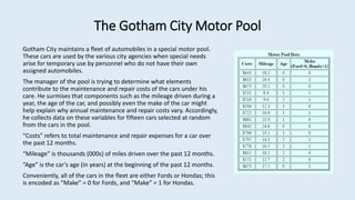
1. The Gotham City Motor Pool
Gotham City maintains a fleet of automobiles in a special motor pool.
These cars are used by the various city agencies when special needs
arise for temporary use by personnel who do not have their own
assigned automobiles.
The manager of the pool is trying to determine what elements
contribute to the maintenance and repair costs of the cars under his
care. He surmises that components such as the mileage driven during a
year, the age of the car, and possibly even the make of the car might
help explain why annual maintenance and repair costs vary. Accordingly,
he collects data on these variables for fifteen cars selected at random
from the cars in the pool.
“Costs” refers to total maintenance and repair expenses for a car over
the past 12 months.
“Mileage” is thousands (000s) of miles driven over the past 12 months.
“Age” is the car’s age (in years) at the beginning of the past 12 months.
Conveniently, all of the cars in the fleet are either Fords or Hondas; this
is encoded as “Make” = 0 for Fords, and “Make” = 1 for Hondas.

2. Looking at One Variable at a Time …

3. (Two-Dimensional) Tables
As a first step in his analysis of these data, the manager
calculates the average maintenance and repair costs for
new, one-year-old, and two-year-old cars. The results are:
• Although he is somewhat surprised by the results, the
manager concludes that the age of the car does not
significantly influence the repair and maintenance costs.
As a next step, the manager calculates the average costs
for each make of car. The results are:
• He concludes that he should, in the future, give
preference to purchasing Hondas since he would save
$52 each per year in maintenance and repairs.
Do you agree with the manager? How would you suggest that he analyze the data? What are your
conclusions?

4. (Two-Dimensional) Tables Show Only Shadows
Not surprisingly, the new cars are more
popular with city employees, and get taken
out more often (and consequently are
driven further) than the older cars during
the year.
And, for whatever reason, the Fords are
more popular, and end up being driven
further than the Hondas during the year.
We need a way to look at all the dimensions of a relationship at the same time. This is what regression
analysis can do!
For example, we’ll see (via regression) that Fords of the same age, and driven the same distance, as
Hondas have maintenance and repair costs, on average, $47 less per year.

5. The Regression “Machine”
The regression model
(terminology, structure,
and assumptions)
relevant sample data
(no missing data)
regression results
(today’s focus)

6. The Regression Model
ε
Make
β
Age
β
Mileage
β
α
Costs 3
2
1 







the
dependent
variable
explanatory variables
or
independent variables
residual term
coefficients linear
mathematical structure
What we’re talking about is sometimes explicitly called “linear regression
analysis,” since it assumes that the underlying relationship is linear (i.e., a
straight line in two dimensions, a plane in three, and so on)!

7. Why Spend All This Time on Such a Limited Tool?
• Some interesting relationships are linear.
• All relationship are locally linear!
• Several of the most commonly encountered nonlinear relationships in
management can be translated into linear relationships, studied using
regression analysis, and the results then untranslated back to the
original problem!

8. A Few Final Assumptions Concerning 
• The validity of regression analysis depends on several assumptions concerning the residual term.
• E[ε] = 0 . This is purely a cosmetic assumption. The estimate of α will include any on-average residual effects
which are different from zero.
• ε varies normally across the population. While a substantive assumption, this is typically true, due to the
Central Limit Theorem, since the residual term is the total of a myriad of other, unidentified explanatory
variables. If this assumption is not correct, all statements regarding confidence intervals for individual
predictions might be invalid.
• The following additional assumptions will be discussed later in the course.
• StdDev[ε] does not vary with the values of the explanatory variables. (This is called the homoskedasticity
assumption.) Again, if this assumption is not correct, all statements regarding confidence intervals for
individual predictions might be invalid.
• ε is uncorrelated with the explanatory variables of the model. The regression analysis will “attribute” as much
of the variation in the dependent variable as it can to the explanatory variables. If some unidentified factor
covaries with one of the explanatory variables, the estimate of that explanatory variable’s coefficient (i.e., the
estimate of its effect in the relationship) will suffer from “specification bias,” since the explanatory variable
will have both its own effect, and some of the effect of the unidentified variable, attributed to it. This is why,
when doing a regression for the purpose of estimating the effect of some explanatory variable on the
dependent variable, we try to work with the most “complete” model possible.

9. What Can Regression
Analysis Do for You?
• Make predictions (based on available information)
• Estimate group means (for similar individuals)
• Measure effects (while controlling for other influences)
• Help evaluate/improve a model (of a relationship)

10. 1. Make a Prediction
For an individual, predict the value of the dependent variable, given the
values of some of the explanatory variables.
• Process: “Regress” the dependent variable onto the given explanatory
variables. Then “Predict.” Fill in the values of the explanatory variables.
Hit the “Predict” button.
• Answer: (prediction) ± (~2)·(standard error of prediction)
• Example: Predict the maintenance cost of a one-year-old car (in the
fleet) which will be driven 18,500 miles over the next year.

11. Make a Prediction
• Predict the annual maintenance cost of a one-year-old car (in the fleet) which
will be driven 18,500 miles over the next year.
• Process: “Regress” Cost onto Mileage and Age. Then “Predict”, filling in 18.5
for Mileage and 1 for Age. Hit the “Predict” button.
• (prediction) ± (~2)·(standard error of prediction)
• $745.60 ± 2.1788·$54.56 (we’re 95%-confident that the prediction is within ±$118.88 of
actual Costs, i.e., actual Costs end up somewhere between $626.74 and $864.47)

12. 2. Estimate a Group Mean
For a group of similar individuals (i.e., individuals with the same values for
several independent variables), estimate the mean value of the dependent
variable.
• Process: “Regress” the dependent variable onto the given explanatory
variables. Then “Predict.” Fill in the values of the explanatory variables. Hit
the “Predict” button.
• Answer: (prediction) ± (~2)·(standard error of estimated mean)
• Example: Estimate the mean annual maintenance cost of two-year-old
Fords (note the plural!) in the fleet.

13. Estimate a Group Mean
• Estimate the mean annual maintenance cost of two-year-old Fords (note the
plural!) in the fleet.
• Process: “Regress” Cost onto Age and Make. Then “Predict”, filling in 2 for Age
and 0 for Make. Hit the “Predict” button.
• (prediction) ± (~2)·(standard error of estimated mean)
• $722.72 ± 2.1788·$59.01

14. Sources of Prediction-Related Error
(a two-slide technical digression)
0
X
b
X
b
a
Y
ε
X
β
X
β
α
Y
k
k
1
1
pred
k
k
1
1












standard error of the
regression, StdDev()
standard error of the
estimated mean
standard error of the
prediction
2
2
this
this
this 

There are two ways in which our prediction (Ypred) for an individual might differ from reality (Y):
reality
the prediction
equation

15. The Standard Error of the Regression
• Using the prediction equation, we
predict for each sample observation.
• The difference between the
prediction and the actual value of
the dependent variable (i.e., the
error) is an estimate of that
individual’s residual.
• StdDev() is estimated from these.
Indeed, the regression “process” simply
finds the coefficient estimates which
minimize the standard error of the
regression (or equivalently, which minimize
the sum of the squared residuals)!

16. 3. Measure a Pure Effect
A one-unit difference in an explanatory variable, when everything else of
relevance remains the same, is typically associated with how large a
difference in the dependent variable?
• Process: “Regress” the dependent variable onto all of the relevant
explanatory variables (i.e., use the “most complete” model available).
• Answer: (coefficient of explanatory variable)
± (~2)·(standard error of coefficient)
• Example: Estimate the “pure” impact of 1,000 miles of driving during the
year on annual maintenance costs.

17. Measure a Pure Effect
• Estimate the “pure” impact of 1,000 miles of driving during the year on
annual maintenance costs.
• Process: “Regress” Costs onto Mileage, Age, and Make (i.e., use the “most
complete” model available, so Age and Make can be held constant).
• (coefficient of explanatory variable) ± (~2)·(standard error of coefficient)
• $29.65 ± 2.2010·$3.92

18. 4. Modelling: Why Does The Dependent Variable Vary?
What fraction of the variance in the dependent variable (from one individual
to another) can potentially be explained by the fact that the explanatory
variables in our model vary (from one individual to another)?
• Process: “Regress” the dependent variable onto the explanatory variables
currently under consideration. Then look at the “adjusted coefficient of
determination” (synonymously, “the adjusted r-squared”).
• Example: Why does annual maintenance expense vary across the cars in
the fleet?

19. Why Does The Dependent Variable Vary?
• Why does annual maintenance expense vary across the cars in the fleet?
• Partial Answer: Because Mileage, Age, and Make vary across the fleet.
• How much of an answer is that? Regress Costs onto those three variables.
Variation in Mileage, Age, and Make
can potentially explain 80.78% of the
variation in Costs. The other 19.22% of
the variation must be explained by
other unidentified variables still
lumped together in the residual term.

20. Why Does The Dependent Variable Vary?
• Why does annual maintenance expense vary across the cars in the fleet?
• Variation in Mileage alone can explain 56.26% of the variation in Costs.
• Variation in Age alone can explain nothing (read “0%” for negative values*).
• Variation in the two together can explain 78.09% of the variation in Costs.

21. The Explanatory Power of the Model
• Names can vary: The {adjusted, corrected, unbiased} {coefficient of
determination, r-squared} all refer to the same thing.
• Without an adjective, the {coefficient of determination, r-squared} refers to a
number slightly larger than the “correct” number, and is a throwback to pre-
computer days.
• When a new variable is added to a model, which actually contributes
nothing to the model (i.e., its true coefficient is 0), the adjusted coefficient
of determination will, on average, remain unchanged.
• Depending on chance, it might go up or down a bit.
• *If negative, interpret it as 0%.
• The thing without the adjective will always go up. That’s obviously not quite “right.”

22. Modelling: Relative Explanatory Importance
Considering a set of explanatory variables, rank them in order of importance
in helping to explain why the dependent variable varies.
• Process: “Regress” the dependent variable onto the target set of
explanatory variables. Rank the variables in order of the absolute values of
their beta-weights, from largest (most important in explaining variation in
the dependent variable) to smallest (least important in explaining variation.
• Example: Rank Mileage, Age, and Make in order of relative importance in
helping to explain why Costs vary across the fleet.

23. 5. Modelling: Relative Explanatory Importance
• Rank Mileage, Age, and Make in order of relative importance in helping to
explain why Costs vary across the fleet.
• One standard-deviation’s-worth of variation in Mileage is associated with
1.1531 standard-deviation’s-worth of variation in Costs.
• One standard-deviation’s-worth of variation in Age is associated with
0.5567 standard-deviation’s-worth of variation in Costs.
• One standard-deviation’s-worth of variation in Make is associated with
0.2193 standard-deviation’s-worth of variation in Costs.
Therefore, variation in Mileage is more
than twice as important as is variation in
Age (and more than five times as
important as is the fact that some cars in
the fleet are Fords, and others are
Hondas) in helping to explain why Costs
vary (when all three of those variables are
considered together).

24. The Beta-Weights
• You can’t compare regression coefficients directly, since they may carry
different dimensions.
• The beta-weights are dimensionless, and combine how much each
explanatory variable varies, with how much that variability leads to
variability in the dependent variable.
• Specifically, they are the product of each explanatory variable’s standard deviation
(how much it varies) and its coefficient (how much its variation affects the
dependent variable), divided by the standard deviation of the dependent variable
(just to remove all dimensionality).

25. End of Session 1

26. 6. Modelling: Which Variables “Belong”
in the (Current) Model?
How strong is the evidence that each explanatory variable has a non-zero
coefficient (i.e., plays a predictive role) in the current model?
• Process: “Regress” the dependent variable onto the (current) set of explanatory
variables. For each explanatory variable, examine the “significance level”
(synonymously, the “p-value”) of the sample data with respect to the null
hypothesis that the true coefficient of that variable is zero.
• The closer the significance level is to 0%, the stronger is the evidence against that null
hypothesis (i.e., the stronger is the evidence that this variable does indeed belong in the
current model).
• Example: How strong is the evidence that Mileage, Age, and Make each “belong”
in the model which predicts Costs from all three?

27. Which Variables “Belong” in the (Current) Model?
• How strong is the evidence that Mileage, Age, and Make each “belong” in
the model which predicts Costs from all three?
• For Mileage and Age, “overwhelmingly strong”.
• For Make, a “little bit of supporting evidence”, but not even “moderately strong”.
• With more data, if the true coefficient of Make is
non-zero, the significance level will move towards
0%, and the evidence for inclusion will be stronger.
• With more data, if the true coefficient of Make is
really zero, the significance level will stay well above
0%, and the estimate of the coefficient will move
towards 0 (the “truth”).

28. Modelling: Detection of Modelling Issues
Is a linear model appropriate?
• Judgment (non-statistical)
• Residual analysis (non-statistical)
• Residual plots
• Against explanatory variables
• Against predicted values
• Outlier analysis

29. Modelling: What is the Structure of the Relationship?
Is a linear model appropriate? Are there alternatives?
• Interactions
• Other nonlinearities
• Quadratic
• Logarithmic – post-course
• In explanatory variables
• In the dependent variable
• Qualitative variables
• Explanatory
• Dependent – post-course