Analysis of Cross-ply Laminate composite under UD load based on CLPT by Ansys...
MECHANICS OF COATED MEMBRANES
1. AFRL-DE-TR-2002-1063, Vol. II AFRL-DE-TR-
2002-1063, Vol. n
MECHANICS OF A NEAR NET-SHAPE STRESS-
COATED MEMBRANE
Volume n of II
BOUNDARY VALUE PROBLEMS AND SOLUTIONS
James M. Wilkes
June 2003
Final Report
AIR FORCE RESEARCH LABORATORY
Directed Energy Directorate
3550 Aberdeen Ave SE
AIR FORCE MATERIEL COMMAND
KIRTLAND AIR FORCE BASE, NM 87117-5776
200311U 022
2. Using Government drawings, specifications, or other data included in this document for any
purpose other than Government procurement does not in any way obhgate the U.S.
Government. The fact that the Government formulated or supplied the drawings,
specifications, or other data, does not license the holder or any other person or corporation; or
convey any rights or permission to manufacture, use, or sell any patented invention that may
relate to them.
This report has been reviewed by the Public Affairs Office and is releasable to the National
Technical Information Service (NTIS). At NTIS, it will be available to the general public,
including foreign nationals.
Ifyou change your address, wish to be removed from this mailing list, or your organization no
longer employs the addressee, please notify AFRL/DEBS, 3550 Aberdeen Ave SE, Kirtland
AFB,NM 87117-5776.
Do not return copies of this report unless contractual obligations or notice on a specific
document requires its return.
This report has been approved for publication.
//signed//
RICHARD A. CARRERAS
Project Manager
//signed// //signed//
JEFFREY B. MARTIN, Lt Col, USAF THOMAS A. BUTER, Col, USAF
Chief, DEBS Deputy Director, Directed Energy Directorate
3. REPORT DOCUMENTATION PAGE
Form Approved
0MB No. 0704-0188
Public reDorting burden for this collection of information is estimated to average 1 hour per response, including the time for reviewing instructions, searching existing data sources, gathenng and maintaining the
data needed and completing and reviewing this collection of infomTatlon. Send comments regarding this burden estimate or any other aspect of this collection of information including suggestions for redua
this burden to Department of Defense, Washington Headquarters Services, Directorate for Information Operations and Reports (0704-0188), 1215 Jefferson Davis Highway, Suite 1204, Arlington, VA 22202-
4302 Respondents should be aware that notwithstanding any other provision of law, no person shall be subject to any penalty for falling to comply with a collection of information if it does not display a cunrently
valid 0MB control number. PLEASE DO NOT RETURN YOUR FORM TO THE ABOVE ADDRESS.
1. REPORT DATE (DD-MM-YYYY)
12-06-2003
2. REPORT TYPE
Final Report
4. TITLE AND SUBTITLE
Mechanics of a Near Net-Shape Stress-Coated Membrane
Volume II: Boundary Value Problems and Solutions
6. AUTHOR{S)
James M. Wilkes
7. PERFORMING ORGANIZATION NAME{S) AND ADDRESS(ES)
Air Force Research Laboratory/DEBS
3550 Aberdeen Ave SE
Kirtland AFB, NM 87117-5776
9. SPONSORING / MONITORING AGENCY NAME(S) AND ADDRESS{ES)
Air Force Office of Scientific Research
801 North Randolph Street, Room 732
Arlington, VA 22203-1977
12. DISTRIBUTION / AVAILABILITY STATEMENT
Approved for public release; distribution limited.
3. DATES COVERED (From - To)
Oct 2000 - Jun 2003
5a. CONTRACT NUMBER
5b. GRANT NUMBER
5c. PROGRAM ELEMENT NUMBER
61102F
5d. PROJECT NUMBER
2302
5e. TASK NUMBER
BM
5f. WORK UNIT NUMBER
03
8. PERFORMING ORGANIZATION REPORT
NUMBER
AFRL-DE-TR-2002-1063, Volume
II of II
10. SPONSOR/MONITOR'S ACRONYM(S)
11. SPONSOR/MONITOR'S REPORT
NUMBER(S)
13. SUPPLEMENTARY NOTES
14. ABSTRACT
This report is the sequel to Volume I of the same title, in which asymptotic methods were used to denve theories that would
aid in understanding the mechanical behavior of a stress-coated membrane. In Volume II we have applied those theories to a
number of boundary value problems, obtaining generalizations of well-known solutions for a membrane, plate, or shell of a
single material to solutions for the same structure, but now consisting of a multilayer-coated polymer material. Perhaps the
most significant accomplishment of this work was the discovery of simple prescriptions for the coating stress that would
maintain the shape of an initially parabolic coated membrane after removal from the mold upon which it was cast. These
solutions involve linear combinations of Kelvin functions. Coating prescriptions are given for membrane laminates both with,
and without, pressure and gravitational loads. The prescriptions are presently being used in the preliminary design of a near
net-shaped stress-coated membrane, to be demonstrated hopefully in the near future.
15. SUBJECT TERMS
Membrane mirrors, optical stress coatings, composite material mechanics, plate and shell
theory
16. SECURITY CLASSIFICATION OF:
a. REPORT
Unclassified
b. ABSTRACT
Unclassified
c. THIS PAGE
Unclassified
17. LIMITATION
OF ABSTRACT
Unlimited
18. NUMBER
OF PAGES
82
19a. NAME OF RESPONSIBLE PERSON
James M. Wilkes
19b. TELEPHONE NUMBER (include area
code)
505-846-4752
Standard Form 298 (Rev. 8-98)
Prescribed by ANSI Std. 239.18
4.
5. Contents
1 Introduction 1
2 Geometrically Linear Membrane Laminate Problems 5
2.1 Pressurized Membrane Laminate with 0-Dependent Boundary 5
2.2 Vibrations of a Membrane Laminate 7
3 Geometrically Nonlinear Membrane Laminate Problems 8
3.1 Reduction to an Axisymmetric System 9
3.2 Generalization of Hencky-Campbell Theory to a Membrane Laminate 10
3.3 Applications to Bulge Testing 13
4 Geometrically Linear Shell Laminate Problems 18
4.1 Reduction to an Axisymmetric System 19
4.2 General Solution for an Initially Parabolic Coated Membrane Laminate 23
4.2.1 Computing the Kelvin Functions 28
4.2.2 Free Edge, Simply-Supported at the Center 29
4.2.3 Pinned, or Hinged, Edge 32
4.2.4 Rigidly Clamped Edge, and Coating Stress Prescriptions for Maintaining an Initially
Parabolic Shape 34
4.3 General Solution for an Initially Flat Laminate 37
4.3.1 Flat Pressurized Laminate, Clamped at the Edge 39
4.3.2 Unpressurized Laminate with Free Edge: Generalized Stoney Formula 41
5 Geometrically Nonlinear Shell Laminate Problems 44
5.1 Reduction to an Axisymmetric System 46
5.2 Approximate Solutions for Initially Flat Laminates Using Perturbation Methods 49
5.2.1 Pressure Versus Axial Displacement Curves 49
5.2.2 BuckHng Due to Compressive Intrinsic Stress Loads 58
5.3 Power Series Solutions 60
5.3.1 Scale-Invariant Functions and Constants 64
6 Conclusions 65
A Elementary Analysis of Stress and Strain Due to CTE Mismatch Between Membrane
and Mandrel 66
m
6. List of Figures
1 Definition of the reference configuration S (upper part of Figure) of a coated membrane shell
of revolution as a mapping from the reference placement C (lower part of Figure), assuming
the layer thicknesses to be constant along any line parallel to the axis 2
2 Reference placement C of an A^'-layer stack 3
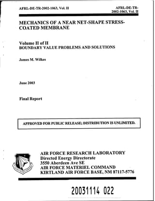
3 Comparisons of WQ versus p, using equation (3.63), to results using the finite element method.
These plots are for AT = 0 (hence also T = f = 0), i.e., for zero net residual stress in the
coated membrane laminate 14
4 T versus CQ for five values oi UA 16
5 Comparison of membrane laminate theory, equation (3.63), with curve generated by equation
(1) of Bahr, et al [14], assuming Si = <Tr = 117 MPa in each coating layer i 17
6 Comparison of theory to geometrically linear FE u-displacement results (free edge/simply-
supported at the center) 32
7 Comparison of theory to geometrically linear FE u;-displacement results (free edge/simply-
supported at the center) 33
8 Comparison of theory to geometrically linear FE u-displacement results (pinned edge) 34
9 Comparison of theory to geometrically linear FE ^-displacement results (pinned edge) 35
10 Comparison of theory and finite element results for radial displacement u{R) when the coating
stress is 1% off-design 3g
11 Comparison of theory and finite element results for axial displacement w{R) when the coating
stress is 1% off-design 37
12 Comparison of theory and finite element results for radial displacement u{R) when the coating
stress is 10% off-design 3g
13 Comparison of theory and finite element results for axial displacement w{R) when the coating
stress is 10% off-design 3g
14 Comparison of theory and finite element results for apex displacement w{0) as a function of
the percent that coating stress is off-design 40
15 Absolute value IA:| as a function of thickness of outer Si02 dielectric coating layer 43
16 Radial edge displacement u{a) as a function of thickness of outer Si02 dielectric coating layer. 44
IV
7. List of Tables
1 Comparison of thickness-weighted averages with values occurring in the geometrically nonlin-
ear membrane laminate theory 17
9. 1 Introduction
A companion [1] to this Report discusses motivation for the analysis of near net-shape stress-coated mem-
branes, and presents details of the derivations of four different theories of the mechanics of such a laminate
using the method of asymptotic expansions. Our goals here are to present solutions of selected boundary
value problems, and to compare the results with those obtained by the finite element (FE) method where
available. Each of the next four Sections will be organized in a similar way, i.e., the governing equations for a
given theory will first be restated from Reference [1], boundary conditions will then be imposed, and details
of the solution procedure for each such set of boundary conditions will be presented. Finally, graphical
comparisons will be made between the solutions of a given boundary value problem, and those using FE
analysis.
With regard to nomenclature and notation, all problems presented here involve an A^-layer structure
consisting of a membrane substrate of thickness HN = hg having A^ - 1 coatings with thicknesses hi, i =
1,...,7V - 1, and total thickness h = hg + he, where he = J2k=i hk is the total coating thickness. This
structure has a circular boundary of radius a. The reference configuration S of the coated membrane is
defined by a mapping from a purely geometrical region C, which we refer to as the reference placement. This
mapping is illustrated for a single coating in Figure 2 of Reference [1], and reproduced below as Figure 1.
As shown in the Figure, the coating and membrane thicknesses are assumed to be constant along any line
parallel to the axis. The reference placement for iV - 1 coatings is illustrated in Figure 5 of Reference [1],
and reproduced below as Figure 2. Note that the coatings are "on the bottom". The basis of this rather
counterintuitive orientation is the optical convention that the direction of propagation of light, which strikes
the coating first, coincides with the positive Z-direction (upward in our Figures). The coordinate ^ = Z+h/2
shown in Figure 2 is convenient for labehng the top and bottom surfaces of each layer, and we note from
Figure 2 the important relation ^i = Yll^i hk.
The following constants appear in the through-the-thickness integrals of the constitutive relations defining
the stress resultants and stress couples, treated in detail in Appendix A of [1]:
N .. 7V-1 N
^f = J2hiSi, M = -^ Yl hihk{Si-Sk), (1.1)
i=l k = i+l
N N
A = J2 ^iQi' ^"^Y. '^^'^i'^i, (1-2)
i=: 1=1
^ N-l N ^ N-1 N
1 = 1 fe = i+l ' i= k = i--
N 1 N- N
i=l i— k = i+l
1 ^ r 1
^ = ^ E ^^ '^n'^i + 3 (ft - hif - i2^i_i {h - ^oj, (1-5)
j=l
D, = ^YQiUi hi [/i2 + 3 (/i - hif - U^i-i {h - ii) , (1.6)
i=l
N
Z?e = ^ ^ Gi fti [hi + 3 (ft - hif - 12^i_i (ft - ii^ , (1.7)
12. ,t=i
10. Surface of Mold
h.
he
Mapping (p: R = R,e = e,Z = T(R) + Z
"^y^
P
z
O R S
Z = hl2
Z = 0
Z = {hc- h.)/2
Z = -A/2
Figure 1: Definition of the reference configuration S (upper part of Figure) of a coated membrane shell of
revolution as a mapping from the reference placement C (lower part of Figure), assuming the layer thicknesses
to be constant along any line parallel to the axis.
where, in (1.1), Si is the residual stress load in layer i. The elastic constants of the material in each layer
appear in the forms
Qi^ ^'1-1/2'
Gi =
l + Vi'
(1.8)
where Ei and Vi are Young's modulus and Poisson's ratio for material i. The area! density of the coated
membrane (ma^s per unit area of the circular disk perpendicular to the axis; units of kg/m^) is defined and
11. ^ I.
^N - tl
{hN,EN,U]^i,SN) N
{hff-i, -Bjv-i, I'Ar-i, 5jv_i) N -1
t = h/2 (D
^i
(hi,Ei,Ui,Si) i
^i-i
6
{hx,EuVuSi) 1
Z = hl2
Z = 0
6 = 0 7 = -h/2
Figure 2: Reference placement C of an iV-layer stack.
denoted by
N
70 = 2_j ^iPOii (1.9)
i=l
where poi is the volume mass density of the material in layer i. The external loads are the pressure difference
p = p- -p^ between the two faces of the coated membrane, and the gravitational body force 70 g (where g
is the gravitational acceleration) in the positive axial direction (up) of our two Figures.
We realized only after the publication of Ref. [1] that the nine A, B^sxidD coefficients were not inde-
pendent. We in fact find the following three relations between the multilayer coefficients (recall that each
layer is assumed to be uniform, homogeneous, and isotropic in its material properties):
Ae = A- A^, Be = B - B^, DQ = D - D^. (1.10)
Similar to Jones [2, p. 155], we refer to A as the extensional stiffness, B as the coupling stiffness, and D
as the bending stiffness of the multilayer laminate. It is convenient to also introduce extensional, coupling,
and bending Poisson's ratios defined by
UA =
A,
VB —, and VD =
D'
(1.11)
12. respectively. Note that for a single layer with Poisson's ratio u, or for a multilayer in which all layers have
the same Poisson's ratio f (an unlikely possibility), the three Poisson's ratios defined in (1.11) are all equal
to z/ as well. Equations (1.10) can be written in terms of the stiffnesses and Poisson's ratios as
Ae = A{1 - UA), Be = B {1 - VB) , De = D {I - VD) . (1.12)
The most important initial shape for optical purposes is a paraboloid, so throughout this Report we
consider a membrane cast on a paraboloidal mandrel (also referred to as "the mold"), then coated on the
mandrel, and subsequently released from the mandrel as a near net-shape coated membrane laminate. We
assume that the coated membrane middle surface is governed by the equation
nR) = ij{<^'- R'), (1.13)
where / is the focal length of the reference paraboloid. A flat middle surface is modeled by a paraboloid
having an "infinite" focal length, in which case T{R) = 0. From (1.13), the central (or vertex, or apex)
displacement of the paraboloid is given by
a2
To = r(0) = -, (1.14)
and its slope at any point R is
R
Tfl = -^. (1.15)
The /-number of the paraboloid, which we denote by F*, is defined by
F* ^ I, (1.16)
hence the ratio of apex deflection To to the radius a can be written as
To 1
In the optics literature a paraboloid with (for example) an /-number of 2 is referred to as an //2 paraboloid,
and we indicate this by writing F* = 2. The ratio (1.17) for an //2 paraboloid is 1/16, or 0.0625.
It is often more convenient to write (1.13) in terms of a parameter K defined by
1 1
K = (1.18)2/ 4aF*'
in which case we have
r{R) = 1{a'-R'). (1.19)
Note that the principal curvatures /ci and K2 of the paraboloid are given by
"'= (1-Jii;2)3/2' and K,= (i_7^,),/,, (1.20)
which are equal only at the vertex R = Oof the paraboloid, where KI = K2 = -K. Thus, K is the (negative)
vertex curvature of the paraboloid, and /c -^ 0 as / -^ oo, i.e., as the paraboloid flattens into a plane.
Unless otherwise stated, all variables appearing in this work are leading order functions of the cylindrical
coordinates {R, 6, Z) on the reference placement C. The subscript (0) used to denote leading order variables
in Reference [1] will be omitted in all that follows. Reference [1] should be consulted for further details on
the definitions of the functions appearing in the equations of this Report.
13. 2 Geometrically Linear Membrane Laminate Problems
The simplest of the theories presented in Reference [1] is that of a geometrically linear coated membrane
laminate. It is the only theory for which we consider solutions that are non-axisymmetric. The equations
governing the mechanics of such a laminate are given in § 11 of that Report, which are repeated here, beginning
with the strain-displacement relations, then the integrated through-the-thickness forms of the constitutive
relations, and finally the equilibrium equations stated in terms of stress resultants (stress couples do not
appear in a membrane theory). Throughout this Report, a reference to an equation in [1] will be distinguished
by appending a ".I" extension to the referenced equation number.
2.1 Pressurized Membrane Laminate with 6-Dependent Boundary
For membrane laminates, the leading order displacement components are given by
UR = U, Ue = V, Uz = w, (2.1)
where u, u, and w are functions of R and 0 only. The leading order strain-displacement relations are found
in equations (11.20.I)-(11.22.I), viz.,
4iR = ",«' (2.3)
4e = ^- (2-4)
The stress resultants (11.29.I)-(11.31.I) result from through-the-thickness integrals of the leading order
constitutive relations (11.17.I)-(11.19.I), yielding
NR=N + Aelj,^A,els, (2.5)
iVfle = ^e4e, (2-6)
NQ=M + A,elj, + Ae%Q. (2.7)
Finally, recalUng the definition w(i?) = T{R) -- w{R,Q), the leading order equilibrium equations are given
in terms of the stress resultants by equations (11.26.1)-(11.28.1):
{RNR)J, - Ne + NRe,e = 0, (2.8)
{R'^NRQ)^^ + RNe,e = 0, (2.9)
[R (r,R NR + w,R NR + ^NRe)] + (r,fliVfle + W,RNR@ + ^N@ ) ^ + (p + 70g) i? = 0. (2.10)
We seek solutions of (2.2)-(2.10) for an initally flat coated membrane, so that T^R = 0, and with u = v = 0
for all R. When these hold, we have e^ie = ^RR = ^ee = 0' ^^nce NR = Ne = ^f and NRQ = 0. Equations
(2.8) and (2.9) are then identically satisfied, and (2.10) reduces to
{RW,RJ^),, + {^^f) ^ + iP+ ^o9)R = 0. (2.11)
16. We consider free vibration solutions of (2.26)-(2.28) for which u = v = 0, assuming there is no pressure
load, and ignoring the effects of gravity. We further assume that we have an initally fiat reference configu-
ration, so that r,R = 0. The conditions u = v = 0 again imply €%Q = e^j^ = e%Q = 0, hence NR = Ne = Af
and Nne = 0. Equations (2.26) and (2.27) are then identically satisfied, and (2.28) reduces to
{Rw,RM)f^ + {^^f) ^ = loRw,tt. (2.29)
Assuming M to be constant, we carry out the differentiations in (2.29) to obtain
«/^,Rfi + -^ + -^ = ^«;,„. (2.30)
The left-hand side of (2.30) is the Laplacian of w, hence we can write the equation as
,-,-> 1
V^w - -^w^tt - 0, (2.31)
which is the homogeneous wave equation for an axial displacement having propagation velocity
c = (2.32)
The solutions of (2.31) are well-known (see, for example, [4, p. 635]), and will not be repeated here. However,
the angular frequencies of vibration are given by
c / Af
(^mn = ^'"" - = "'nn W ;^ , (2.33)
where a is the membrane radius, and amn is the mth positive zero of the ordinary Bessel function J„ of
order n (n = 0,1,2,...), i.e., Qm„ is a solution of the equation Jn{amn) = 0. Note that the tension T which
appears in the small oscillation theory of a single material "drumhead" is replaced in this theory of a coated
membrane laminate by the net residual stress resultant M defined in equation (1.1).
3 Geometrically Nonlinear Membrane Laminate Problems
The leading order strain-displacement relations are given by equations (9.27.I)-(9.29.I), which contain non-
Unear terms in the axial displacement derivatives:
'«Q-2 i^'« + —R- + ^ + —R^j' (3-1)
4fi = ",fi + r,fli(;,fl -I- - {w^Rf,
2
(3.2)
,0 _ v,e + u jw^ef
R 2/?2^ee = —5— + -iT^r- (3-3)
The stress resultants and equilibrium equations are given by equations (9.33.I)-(9.38.I), which are the same
as those of the previous §2:
NR = Af + Ae°RR + A^e%e, (3.4)
17. NRe = Aeele, (3.5)
Ne =^f + A,e% + Ae%e- (3-6)
and
{RNR)ji - Ne + NR@,e = 0, (3.7)
{R^NRe)j^ + RNe,& = 0, (3.8)
[R (T,RNR + W,RNR +'^NRe)] ^ + [T^RNRQ + W^RNRQ + ^-^e) ^ + {p + 7o9)R = 0. (3.9)
3.1 Reduction to an Axisymmetric System
We specialize immediately to the case of an axisymmetric system by assuming that none of the variables
depend on the angular coordinate 0. Thus, all terms involving partial derivatives with respect to 6 vanish,
leaving the following simplified set of strain-displacement relations and equihbrium equations:
4e = 1 (.,. - I) , (310)
%e — p^ (3.12)
{RNR)I, - Ne = 0, (3.13)
{R'NRe),, = 0, (3.14)
[R{T,RNR + w,RNR)]j^ + ip + ^o9)R = 0. (3.15)
Equations (3.14) and (3.15) can be integrated once to obtain
R^NRQ = CRQ, (3.16)
and
R{T,RNR + W,RNR) + (p + 7off)Y = '^«' ^^-^^^
where CRB and CR are arbitrary integration constants. We must set both of these constants equal to zero
to insure that both NRB and NR are regular at the origin R = 0. Thus, (3.16) and (3.17) reduce to
NRQ = 0, for all R. (3.18)
p
T,RNR + W,RNR + (p + ^og)- = 0. - (3.19)
18. Prom (3.18), (3.5) and (3.10) it then follows that
4e = 2 (^.-R ~ ^) = ^' (3-20)
since ^e is in general nonzero. Equation (3.20) is easily solved to obtain v{R) = VQR, where VQ is an arbitrary
constant. We observe that if v vanishes for any non-zero value of R, say RQ ^ 0, then v{Ro) = VQRO = 0,
hence t;o = 0, and so v vanishes for all R.
The system of equations that remains to be solved is then
e°RR = UR + r,flw,fi + - {w,Rf, e%Q = ^, (3.21)
NR = ^f + Ae''nn + A, ele, (3.22)
Ne =^f + A,elji + A€%Q, (3.23)
iRNR),R - Ne = 0, (3.24)
R
T,RNR + W^RNR + (p + -yog) - = 0. (3.25)
3.2 Generalization of Hencky-Campbell Theory to a Membrane Laminate
We continue the reduction by specializing now to an initially flat coated membrane, so that r,^ = 0, reducing
the system of equations to
^RR = UR+ - {w,Rf, e%Q = ^, (3.26)
NR = J^ + Ae% + A, e%Q, (3.27)
Ne =Af + A^ e°RR + Ae%Q, (3.28)
iR^n),R - Ne = 0 ^ Ne = NR + RNR^R, (3.29)
R
'W,RNR + (p + 70 5) - =0. (3.30)
This system is augmented by the usual compatibility condition obtained by eliminating u between the two
strain-displacement relations (3.26), yielding (see, for example, [5]):
P^O — ,0 0 1 / 2
^^ee,R - ^RR - ^ee - o ^^.^^ ■2 (3.31)
We proceed by introducing a dimensionless coordinate p and dimensionless displacement components u
and w defined by
_ R ^ u ^ w
p=-, u^-, rv^-, (3.32)
10
19. together with the following dimensionless constants:
I'A =
A' h^' '"' ' Eh'
and two new dimensionless dependent variables Xr and xe defined by
_ {p + log)a
Eh
^'' ~ Eh '
Xe
Ne-Af
Eh
(3.33)
(3.34)
Note that UA is the extensional Poisson's ratio defined earlier in (1.11), while E acts as the "eSective"
Young's modulus of the coated membrane laminate. Equations (3.26)-(3.31) can be rewritten in terms of
these dimensionless quantities as
4iJ = u,p + ^w^,
,0
(3.35)
xe = [Y^^J ^^®® "^ "A^RR) '
Xe = Xr + pXr,p = {pXr)^p,
w,p {j + Xr) + q-= Q.
0 0 0 '*^2
P^ee,p — ^RR ~ %e ~ o'^,/"
(3.36)
(3.37)
(3.38)
(3.39)
(3.40)
These equations have precisely the same form as Campbell's [6] equations, which are themselves modifications
of Hencky's [7] membrane equations to allow for an initial tension in the pressurized membrane. Equations
(3.36) and (3.37) are easily inverted to obtain
^RR = Xr - VAXe,
^0S — 2;e — VA Xr,
(3.41)
(3.42)
which, together with (3.38), can be substituted in (3.40) to get the compatibility condition in terms of Xr
and xg:
p (Xr + X0)p =- - -^i^,p- (3.43)
We now use Equation (3.39) to eliminate w^p in equation (3.43), yielding the following equation involving
only the x's:
(r + Xr)
It is convenient here to rescale r, Xr, xe, and w, i.e., we set
{Xr + Xe)
r=i.^/^x. Xr — j Q Xr, Xe
+ ^ = 0.
■q'/'xe, w — q^/^ w
to write equations (3.39) and (3.44) as
w^p (r + Xr) + 2p = 0,
(3.44)
(3.45)
(3.46)
11
20. and
(r + Xrf
i^r + xe)
+ 8 = 0, (3.47)
respectively.
We assume a power series solution for Xr{p), and find after some numerical experimentation that only
even powers of p will contribute. It is convenient to write the series in the form
= -T + 6o(l + X^62np'").
n=l
Prom this and the second equality of (3.38) it follows that
Xe = {pxr)p = -T + 6o
The sum of the last two equations yields
Xr + Xg = -2f -- 26o
1 + 5](2n + l)62„p^"
n=l
l + ^(n+l)62„^2n
n=l
hence, noting that r is a constant,
{Xr + Xe)
= 46oX]n(n + l)62nP^""
n=l
(3.48)
(3.49)
(3.50)
(3.51)
This expression, together with (3.48), is now substituted in (3.47), and the coefficients bzn, n > 1, are then
determined by equating to zero the coefficients of like powers of p. We find, using the Mathematica computer
algebra system, that 62„ is given in terms of 6o by
I,3r
where the ^2n are purely numerical coefficients given, for 1 < n < 9, by
A = i, A = |. ft = g. ft = H
^2 =
1205
567' P14
219241
63504 ' P:16
6634069
1143072'
. 51523763
Pl8 ^= .
5143824
(3.52)
(3.53)
In order to determine the coefficient bo (in terms of which all the other coefficients 62„ can be calculated),
we must impose boundary conditions.
We consider here a clamped boundary, requiring u{a) = 0 and w{a) = 0, or equivalently, 2(1) = 0 and
u;(l) = 0. From the second equation of (3.35), together with equation (3.42), we have the following power
series representation for u:
2(p) = pe%Q = p {xe - VAXr) = jq^'^p -f{l-VA) + ho{-VA)+boY^{2n + l-VA) 62„/J^"
n=l
(3.54)
Applying to this expression the boundary condition on G at p = 1 yields an equation which must be solved
numerically for bo:
1-^
1 - i^^ + ^ (2n + 1 - i/^ ) 62n
n=l
{1-VA)T = 0. (3.55)
12
21. After determining 6oi which in general can be seen from (3.55) to depend on both UA and r, the series
solution for the radial displacement u{p) is given by (3.54).
The dimensionless axial component of displacement w{p) can be obtained by assuming an even power
series of the form oo
^(P) = E^2nP'", (3.56)
n=0
the derivative of which is
2 5]nc2„/92"-i. (3.57)
n=0
This is substituted, together with (3.48) and (3.51), in (3.46), to obtain an equation from which the coeffi-
cients C2„, n > 1, can be determined by comparing like powers of p. Again using the Mathematica computer
algebra system, we find the coefficients C2n, " > 1, to be given in terms of bo by
c^n = -^bl, n>l, (3.58)
where the 72n are purely numerical coefficients given, for 1 < n < 9, by
1 5 55 7
72 = 1, 74 = 2' Te = 9' 78 = ^) 7io - g,
_ 205 _ 17051 _ 2864485 _ 103863265
'^^^ ~ 108' '^^^ ~ "5292"' '^^^ ~ 508032 ' ^^^ ~ 10287648 '
(3.59)
The remaining constant co is determined by the clamped edge boundary condition w{l) = 0, hence from
(3.56):
oo oo
co = -^C2„=6^E|?- (3.60)
n=l n=l 0
After determining CQ, the dimensionless axial displacement component w{p) is given by the power se-
ries (3.56).
Power series solutions for the displacement components (as well as the stress and strain components)
having the proper physical units can be obtained by restoring the scale factors introduced in equations
(3.32), (3.34), and (3.45). For example.
u{R) = auiR/a) = p'^^^R -T{1-UA) + bo{l-UA) + boJ2i^'^ + '^-''A) &2„(i?/a)^"
n=l
(3.61)
and
wiR) = aw{R/a) = aq^^^w{R/a) = aq^'^ ^ c^niR/a)^'', (3.62)
n=0
and the apex deflection WQ = w{0) is, from (3.62):
Wo = aq^l^co. (3.63)
3.3 Applications to Bulge Testing
The last equation (3.63) is useful for the analysis of data obtained from bulge testing (see, for example, [8,
9, 10] for descriptions of such tests), a method under consideration for experimental determination of the
intrinsic coating stress. A brief discussion of such an analysis will follow, but first we compare graphs of
apex deflection versus pressure, using (3.63), to those obtained from FE analysis. Figure 3 shows the results
when N = 0, i.e., for a zero net residual stress resultant. The coated membrane radius here is a = 3.0
13
22. c
E
u
oa
■5.
Apex Displacement -vs- Pressure
T = 0 (zero net intrinsic stress), Diameter = 6.0 in
FE pinned boundary
FE clamped boundary
Membrane laminate theory
0.4 0.6
Pressure p (psi)
0.8
Figure 3: Comparisons of WQ versus p, using equation (3.63), to results using the finite element method.
These plots are for AT = 0 (hence also r = r = 0), i.e., for zero net residual stress in the coated membrane
laminate.
inches = 0.0762 m, the coating and membrane thicknesses are hi = he = 1 fixn and h2 = h^ = 20/im,
respectively, with Ec = 44.0 GPa and E, = 2.2 GPa. The two Poisson's ratios have been assumed the same]
i.e., i/c = I's = 0.4. FE results for both pinned edge and clamped edge boundary conditions (see §4.2.3 for
the definition of pinned edge boundary conditions), treating the coated membrane as a "plate", are also
shown in Figure 3. It is clear from these plots that the results of the theory under consideration resemble
more closely the FE results for a plate with a pinned boundary rather than one with a clamped boundary.
We interpret this to mean that the coated membrane behaves more like a plate than a "true membrane", i.e.,
the bending stiffness of the coated membrane is large enough in this example that a geometrically nonlinear
plate theory is probably necessary to obtain agreement with the FE clamped edge results.
Returning to the subject of bulging tests, we recall that in such tests the apex deflection ("bulge") WQ is
measured as the pressure load p is varied. The analysis of data obtained in this way often relies on a formula
proposed by Beams [8] (see, for example, [9, p. 254], cited in the recent book by Ohring [10, p. 716]). Beams
cites for this formula apparently unpublished work by Cabrera. The derivation of the formula is not given
in [8], and it was used there and in [9, 11] only to analyze thin films of a single material, not a laminate.
A similar formula was given in [12] for applications to square and rectangular films of a single material.
These formulas seem to be intended for applications to "true membranes", since they do not include bending
stiffness. The formula given by Beams [8], expressed in our notation (Beams' application was to a single
thin film of gold), is:
_ .h WQ
a a
n^l equation (2) of [8], (3.64)
14
23. where To is referred to as the "tension" by Beams, but has units of stress and corresponds to omJ^/h. Since
Poisson's ratio for gold is approximately 0.4, for Beams' application equation (3.64) can be rewritten as
ip = i^Af + 4.MEh^, M = hTo. (3.65)
For a single material, in which case E = E, the two terms of the Beams/Cabrera formula follow as an
approximation of our theory by investigating the apex deflection as a function of pressure in the two Umiting
cases of zero residual stress, and large residual stress. For zero residual stress {^f = 0), equation (3.63)
applies, where co is a function of Poisson's ratio only, which we find to have the value 0.626 for i/ = 0.4, i.e.,
u;o = 0.626a(|^)'^', AT = 0, u = OA. (3.66)
On the other hand, for large values of A^, i.e., of r, the coefficient 6o in (3.60) is found to be large, so that
Co w l/6o. In this case it also follows from (3.55) that bo « r, hence CQ « 1/T and from (3.63)
,1/3
Wo fti a—zr
T
But from (3.45), r = Ar/q^^^, which yields
Wo « ^9 = JT^P, -^ large, (3.67)
where we used (3.45) again to replace q and r. Thus, for large Af, Wo is linear with pressure p. Equations
(3.67) and (3.66) yield two expressions for the pressure as a function of u;o:
Pi«4^A^, AT large, (3.68)
and g
P2 =A.08 Eh^, M = Q, z/ = 0.4, (3.69)
respectively. The Beams/Cabrera formula (3.65) is obtained as a simple hnear combination of these expres-
sions for pi and P2, viz.,
P = Pi + 4^P2- (3-70)
Since this formula is an approximation, it is expected not to be as accurate in determining the intrinsic stress
as one determined from the exact theory. A more systematic derivation of Beams/Cabrera-Hke formulae using
perturbation techniques will be given later in §5.2.
Our algorithm for using the theory to compute the coating stress Sc in a single-layer coating from bulge
test data is the following. For a given pressure p, a measurement of the apex displacement WQ is made. With
p we can compute q from (3.33), and then from (3.63) we have the corresponding value of CQ:
^ = ^- (3-71)
For this value of CQ, we now determine ho by solving, using some numerical method, equation (3.60), i.e.,
oo
-0 - 6^ E 3^ = 0' (3.72)
n=l °0
rather than (3.55). This, in effect, gives us &o as a function of CQ, i.e., 6o(co). Substitution of this value of bo
in (3.55) then gives r as a function of VA and 6o (or, equivalently, CQ):
r{co,VA) = bo
1 °°
1 + 7- r y^i^ri + l-UA) b2„
(1-''^).=1
15
(3.73)
24. T -VS- C
0
10-
8-
6-
4-
2-
-2-
-1 1 L.
— v^ = 0.2
v^ = 0.3
— V =0.5A
V =0.6A
T 1 r -r ' I ' I ' i 1 1 r-
01 0.2 0.3 0.4 0.5 0.6 0.7 0.8 0.9
Figure 4: r versus CQ for five values of I>A-
We assume that the geometrical and material properties of the coating and membrane are known, so that
UA can be calculated from its definition (3.33), and then (3.73) allows us to compute T(CO) for this fixed
value of UA- As the final step, the computed value of r is used in definitions (3.45) and (3.33) to obtain ^f,
fi:om which Sc follows according to definition (1.1), assuming that the membrane substrate residual stress
5, is known. Figure 4 shows the graphs of r(co) versus co for five different values of UA (note that the curve
for UA = 0.3, restricted to the interval 0.1 < co < 0.653, is the inverse of the graph shown in Figure 6 of
Campbell [6]).
In closing this Section, we note that in order to include the bending stiffness of the material, Bonnotte,
et al [13] appended an additional term to a Beams/Cabrera-like formula. They then used FE analysis to
determine two fitting constants appearing in their formula. This model was applied later by Bahr, et al [14]
to a square, five-layer laminate material, by simply replacing E and i/ in the Bonnotte, et al formula with
thickness-weighted "composite" values, i.e..
E = ^ ft; Ei/h, ly = ^hi Vilh, h = Y,hi
i=l
(3.74)
t=i
These composite values appear in their equation (1) only in the combination ^/(l - i/2), which they refer
to as the composite "biaxial modulus", denoted by YB in Bonnotte, et al [13], and by Q in our definition
(1.8). It should be noted in this regard that in other recent literature, e.g., [15, 16, 17], the term "biaxial
modulus" is used instead for the quantity El{-v) (a convention which we shall adopt later, denoting it
by B). For a Poisson's ratio of 0.4 the first definition gives a value of 1.19 £, while the second gives a value
of 1.67 £, roughly 40% higher than the first. In Table 1 we use the Bahr, et al [14] data to compare values
16
25. Table 1: Comparison of thickness-weighted averages with values occurring in the geometrically nonlinear
membrane laminate theory.
E (GPa) V E/(l-i/2) (GPa)
Thickness-weighted averages 145.6 0.280 158.0
Membrane laminate theory 145.8 0.283 158.5
computed using the thickness-weighted averages in (3.74) with those computed using the definitions (3.33)
occurring in the geometrically nonlinear membrane laminate theory. For all practical purposes, the values
obtained by the two different methods are the same in this particular example.
Results obtained with the formulas used in [13] and [14] are probably not comparable to results using our
theory, as their formulas were determined empirically by fitting to data obtained on rectangular specimens,
rather than circular ones. However, ignoring this important distinction for the moment, and using the data
given in [14], we compare in Figure 5 the results of the theory with the results shown in Figure 1 of [14].
Note that their data is for a multilayer consisting of four coating material layers placed on a (fifth) sihcon
Pressure -vs- Apex Displacement
S. = CT =117 MPa in each coating layer i, Diameter = 1.45 mm
1.4e+05r
1.2e+05
le+05
fc- 80000
e 60000
40000 -
20000
T
Membrane laminate theory
Equation (1) of Bahr, et al
I _L
5e-06 le-05 1.5e-05 2e-05
Apex Displacement w^j (m)
2.5e-05 3e-05
Figure 5: Comparison of membrane laminate theory, equation (3.63), with ctirve generated by equation (1)
of Bahr, et al [14], assuming Si = cjr = 117 MPa in each coating layer i.
substrate layer, so that the constants of our theory, defined in equations (1.1)-(1.7), involve TV = 5 layers.
For the theory, we took the radius to be a = 0.725 mm, half that of the side length 1.45 mm of their square
specimens (in [14] this side length is also denoted by a, which should not be confused with our radius a).
In order to match the final point (3 x 10"^ m, 1.4 x 10^ Pa) of their Figure 1 using their equation (1), we
17
26. 1i*n .*S^ r^'' '^''"^"^^ '^'■^'' ""' *° ^^ ^^^ ^^^'^' although they mention the range to be from 90 MPa
to no MPa. Our theoretical curve was generated using equation (3.63), assuming that S. = 117 MPa for
each layer i of the four-layer coating, and Ss = 0 in the substrate. The resulting comparison is reminiscent
of our comparison of the theory and FE analysis in Figure 3, i.e., for a given pressure the theory generally
overestimates the corresponding apex deflection.
4 Geometrically Linear Shell Laminate Problems
For shell laminates, the leading order displacement components are given by the Kirchhoff-Love expressions
UR = u - Zw^R, Ue = V - Z ^, Uz = w, (4.1)
where u.,v, and w are functions of R and 0 only. For a geometrically linear shell laminate, the strain ....
ponents depend linearly on these components and their partial derivatives, according to equations (10 23 I)
(10.28.1) of Reference [1]:
com-
1
= e^e - ZkRQ, (4.2)
tRR = u,fl + T^RW^R - Zw^RR = e°RR - ZkRR, (4.3)
:ee, (4.4)
where the Z-independent strains and curvatures are given by
eRO -2[-,R + —^ + —^) , kRs = -^ + -^, (4.5)
^RR = ",fl + ^,RW,R , kRR = W^RR, (46)
0 _ v,e + u _ w^R ly ee
eee - —^, fcee = -^ + -^. (4.7)
The stress resultants and couples for a shell laminate are given by equations (10.39.I)-(10 44 I) of Refer-
ence [1]: / j
NR = M + Ae% + A,e%Q + B kRR + B^kee, (4.8)
NRQ = AecRQ + BekRe, (4.9)
Ne = Af + A^ 4fl + ^eee + B, kRR + Bkee, (4.10)
MR = -M- Be% - B,e%Q - DkRR - D^kee, (4.11)
MRQ = -Bee^Q - DekRs, (4.12)
Me = -M- B,e% - Be^Q- D^kRR - Dkee, (4.13)
18
28. The remaining system of equations to be solved is then
RNR,R + NR- Ne = 0, (4.26)
RMn,R + MR- Me + RT^RNR + {p + ^^g)^ = O, (4.27)
where
NR = Af + Ae°Rfi + A,e%Q + BkRR + B^feee, (4.28)
Ne= M + A^e% + At%Q + B^HRR + Bkee, (4.29)
MR = -M- B€%fi - 5,4e - DkRR - D.kee, (4.30)
Me = -M- B,e°RR - Be%Q - D.kRR - Dkee, (4.31)
and
fflfl = ",fl + r,fiU;,fl, kRR = W^RR, (4.32)
,0 _ " , W,R
fee -^, Kee = ^ • (4.33)
Next, as in §3.2, we transform these equations to dimensionless forms by introducing a dimensionless
coordinate p, dimensionless displacement components u and w, and a dimensionless initially curved reference
surface T, defined by
p = -, ^ = -. w = -, r = -,
a a a a (4.34)
together with the following dimensionless constants:
„. — " "P - "^ ^1 2 -^ M (p + 700)0
..= ^, E=^{1-.,), r=^^, ,^^^^, .H^%^f (4.35)
and four dimensionless dependent variables Xr,X0,yr, and ye defined by
NR-AT Ne-Af MR + M MQ + M
' Eh ' "^ Eh-' ''- Eha ' ''--Eha ■
(4.36)
We also introduce dimensionless curvatures Kr and Ke defined by
Kr = aA;ij/j = w^pp Ke = akse = —^,
P
(4.37)
and four new dimensionless constants
b- ^ b - ^^ H- ^ W ^-
Eha' " Eha' Eha^' "-Eha''
(4.38)
noting that the strain components are already dimensionless, and have the following forms in
dimensionless variables defined above:
terms of the
4R = Sp + f,pu;,p, e^e = -•
P
(4.39)
20
30. Next, we substitute (4.48) and (4.49) in (4.46) and (4.47) to obtain
3/r = -13Xr - P^xe - 6Kr - 6^Ke, (4.53)
ye = -PuXr - 0xe - S^Kr - Sne, (4.54)
where we introduce another pair of constants:
6 = d - bl3 - huPu, 5^ = d^ - bp„ - h^p. (4.55)
The derivative of yr with respect to p yields from (4.53):
yr,p = -^Xr,p - fi„Xe,p - 6Kr,p - S,,Ke,p. (4.56)
From equations (4.53), (4.54), and (4.56) we obtain
yr,p + -{Vr - ye) = -PXr,p - PuXe^p - S Kr^p - 6^ Kg^p
- -[{0 - P,){Xr - Xe) + {S-6,){Kr -««)].
In this expression, we again use (4.41) to replace (K^ - Ke), and (4.42) to replace {xr - xe), which simplifies
it to
yr,p + -{yr - ye) = -0^ {Xr + Xe) ^^ - 6 {Kr + Ke) ^. (4.57)
Substitution of (4.57) into (4.43) yields the following form of the axial equilibrium equation:
-P^ {Xr + Xe)^p - 6{Kr + Ke )_p + f,p (T + Xr) + q^ = 0. (4.58)
Equation (4.42) can be used to ehminate xe in (4.52) and (4.58), and the problem we are left with is to
solve the coupled differential equations (4.52) and (4.58) for w and Xr. The radial displacement u is then
determined from (4.51).
Equations (4.52) and (4.58) differ in form from those for a shell of a single material only by the terms
involving the coeflficient ^^. Prom its definition, given in (4.50), we note that
Pu = K - VAh = =—- {uB - VA), (4.59)
Eha ^ '
i.e., Pu is proportional to the difference in extensional and coupling Poisson's ratios. This expression can be
expanded, yielding
P. = --±-{AB, - A,B)
Ah, na
, , N N-l N
= TfT;^ 2 ^ ^ 51 ^i^i^k [Qi {QjUj - Qk^k) - QiVi {Qj-Qk)],
i=l j = l k = j+l
which can be manipulated to
N- N-l N1 1 — XJ* — X ft
t=i j = i k = j+i
. ^ ;v-i TV (4.60)
+ —2— ^ ^ ^^^'' ^^^ i^i - ^N) - Qk {vk - VN)] .
j = i k = j+i
22
31. This constant is seen to be a sum of terms, each of which depends upon differences in the Poisson's ratios of
the various material layers. For a single-layer coating of the membrane (hence TV = 2 layers total), we have
simply
KhsQcQs (^^_^j^ (4.61)
2AEa
where i = j = 1 = c in the coating, and fc = 2 = iV = s in the membrane substrate. The total thickness
h = hc + hs disappears from the expression, as it is a common factor in both numerator and denominator.
Thus, if the two materials have the same Poisson's ratio, ,8^ vanishes and the governing equations simpUfy
considerably (this simplifying assumption was made, for example, by Wittrick [18] in his work on the stabiUty
of bimetallic thermostats).
4.2 General Solution for an Initially Parabolic Coated Membrane Laminate
Here, we consider an initially parabolic coated membrane, defined by equation (1.19), viz.,
T{R) = f (a^ - R'),
The dimensionless form of this equation can be written as
r(p) = Y (1 - z'').
where KQ is a dimensionless parameter defined by
UK
a
V'
From (4.63) we obtain
1 ,p — ~Ko p,
which can be substituted in the fundamental equations (4.52) and (4.58) to write them as
[Xr + Xe - Pv (/tr + l^e)]^p - K'o'U},p = 0,
-/?^ [xr + xe)^p - 5 {Kr + Ke )^p - KOP{T + Xr) + q- = 0.
This pair of equations can be uncoupled to obtain a single differential equation for w as follows. Substituting
for {xr + xe)^p from (4.66) into (4.67) yields
(4.62)
(4.63)
(4.64)
(4.65)
(4.66)
(4.67)
-A {Kr + Ke)p - P„KoW^p - KoP {T + Xr) + q-
where we have introduced a new constant A defined by
A = S + Pl = d-{l-ul)b-'.
Solving (4.68) for Xr yields (for KQ ^ 0)
0,
—r
[Kr + KB , ■w.,
^ + Pul^o —
from which
{Kr + Ke ] ,pp
{Kr + Ke )
- Pu
w pp w,,
(4.68)
(4.69)
(4.70)
(4.71)
23
32. FVom equations (4.42), (4.70), and (4.71) we have
Xe = pXr,p + Xr T Ur + Ke)^pp - P^W^pp + -^,
Kn
hence (4.70) and (4.72) yield
n 9 ^
Xr + xe = -2T +
KiQ AC
o L
(«r + HB ).«„ +
(Kr + l^e
PP
IKO''
- Pu I uJ.pp +
t)
We next observe that equation (4.66) can be integrated immediately to obtain
Xr + Xe = Pv (Kr + Kg) + KQ u5 + C3,
where C3 is an arbitrary integration constant. Substituting from (4.73) into (4.74) yields
(«r + Ke )_p
(4.72)
(4.73)
(4.74)
i'^r + Ke )pp + —^— ^ + p^ (wpp + ^ + Kr + Ke) + KoW + 2T - -^ + C3 = 0. (4.75)
Recalling the definition of the p-dependent part of the Laplacian operator in cylindrical coordinates, viz..
V'w = Wpp + ^,
we have
and also
w
Kr + Kg = W^pp + —^ = V^w,
P
V2 (V^u;) = V'w = {V^'w) +
(V^u;)
,pp p
These observations allow us to write equation (4.75) more compactly as
A
Vui + 2/3. ^ V^ti; + |u; = i (g - 2rK„ - C^K,
(4.76)
(4.77)
(4.78)
(4.79)
The complete solution of the linear differential equation (4.79) has the form id{R) = Wh{R)+Wp{R), where
Wh{R) is the general solution of the homogeneous equation
S7'wn + 2I3.'^ V^wn +'^WH = 0, (4.80)
and Wp{R) is a particular solution of (4.79). A suitable particular solution in this case is the constant function
"'P(^) = 72 (9 - 2TKO - C3K0), (4.81)
which involves the as yet unknown integration constant C3. The homogeneous fourth-order linear differential
equation (4.80) has at most four linearly independent solutions. We note that if ip{p) is an eigenfunction of
the p-dependent Laplacian operator defined by (4.76), corresponding to an eigenvalue -m^, i.e., if
VV = -mV, (4.82)
then VV = mV, hence ^ is also a solution of (4.80) ifm satisfies the fourth-degree polynomial equation
m* + 2klm'^ + kf = 0, (4.83)
24
33. where we have introduced two constants fc2 and ki defined by
„2
kl = -/?. 5, kt ^ J, (4.84)
and remark that /3^ can be either positive or negative, while A is always positive. The four solutions of
(4.83) are easily found to be ^
m = ±J-kl ± -^fcT-fef • (4-85)
The forms of these solutions to be used depends on the relation between fc| and kj. We find for typical
parameter values of the material constants and the geometry that kf > kj, so that (4.85) may be written as
m = ±y-fc| ± i^{kl + kl){kl-kl) . (4.86)
This can be put into a more convenient form by introducing two new (real) constants defined by
k = ^Jlikl + kl), e = ^j{kl-kl), (4.87)
which can be inverted to yield fcf and k in terms of e and k:
kl = e-e kl = fc2+e2. (4.88)
The complex eigenvalues (4.86) take the following simple forms in terms of e and k:
m = ±{e±ik). (4.89)
The four distinct eigenvalues rrij, j = 1,2,3,4, are thus given by
mi = e + ik,
m2 = e-ik = ml ^^^^^
ms = - (e 4- ik) = -mi,
m4 = — (e — ik) = ml = —m,2 = -m*,
where an asterisk denotes complex conjugation. These correspond to eigenfunctions ipj{p) satisfying
VVj = -m'V'j, j = 1,2,3,4. (4.91)
Substituting for the Laplacian operator, we obtain the following second-order differential equation for each tpf
xP'J + ^ + m]^j = 0. (4.92)
Introducing new independent (complex) variables ^j = mj p, the jth second-order equation can be written
as
fi
where a prime always denotes the derivative of a function with respect to its argument, in this case ^j, and
ipj{(,j) = ipj{mj p). Equation (4.93) is Bessel's equation of zero order, whose solution regular at the origin
is the zero-order Bessel function Jo(Cj). The general solution of our homogeneous equation (4.80) is then a
linear combination of the four eigenfunctions Jo{^j)-
■Whip) = CiJoimip) + C2 Jo(m2/3) + CsJoimsp) + C4 Jo(m4/?),
= Ci Jo(mip) + CiMmlp) + CsJoi-rriip) + CiJo{-mlp),
25
34. where the arbitrary constants Cj are, in general, complex. Using the fact that Jo is even, i.e., Jo{-z) = Mz)
this homogeneous solution reduces to '
^hip) = CiJoimip) + C2Jo{mlp), (4.95)
where Ci=Ci + C3 and C2 = C2 + d are new arbitrary complex constants. From its definition in (4.90),
we can v^Tite the complex number mi in polar form as
mi = e + ifc = Ve^ + k^ e'*' = k, e'^', ^i = tan-^ (- , (4.96)
where we also used the second equation of (4.88). Equation (4.95) is thus equivalent to
Whip) = CiMe'^'kip) + C2Me-'^'k,p). (4.97)
Now, the ratio k/e defining the angle 9i can be rewritten using (4.87) and (4.84) as
k _ 1 + /?^A-i/2
7 ~ Vl-^.A-V2- (4-98)
We find that for the material and geometric parameters of interest here, it is in fact true that |/9^ A-^/^j jg
always much less than 1 (in a typical case, this product is on the order of 1 x lO'^). We thus approximate
- « 1, =!> Oi K -, (4.99)
which brings (4.97) to the form
^h{p) = CrMe'^'^kip) + C2 Jo(e-'"/''fcip). (4.IOO)
This can be written in terms of Kelvin's her and bei functions (see [19, pp. 379-385], for details of the
properties of the Kelvin functions) as
"5ft(p) = Ci [ber(feip) + ibei(fcip)] + C2 [ber(fcjp) - ibei(ifcip)], (4.IOI)
Since Kelvin's functions are real-_valued, and Whip) must be real, it follows that the complex constants must
in fact be complex conjugates: C2 = Cj. Thus, the general solution for w{p) takes the form
w{p) = Whip) + Wpip) = Ciherikip) + C2bei(fcip) + ^ iq - 2TKO - C3K0), (4.102)
«^
where Ci = Ci + C^ and C2 = i(Ci - CJ) are now arbitrary real constants to be determined from the
boundary conditions.
The dimensionless radial displacement u defined by (4.51) can be expressed in terms of u; and its deriva-
tives as follows. First, we use (4.70) and (4.72) to replace Xr and xe in (4.51), yielding
From (4.79) and (4.78) we obtain the following expression for (V^u;) :
(V^w) 2
26
35. which is substituted for (V^iy) in the previous equation to obtain the desired result, viz.,
,pp
u{p)
V 2KO
{1 + VA) + C^
A
P + {1 + VA) — (V^u?)
+ [P^{2 + VA) - P]w,p + Kopw. (4.103)
To get the derivatives of w{p) appearing in (4.103), in terms of Kelvin functions, we note that
WAP) = ^1 [Ciber'(fcip) + C72bei'(fci;o)] , (4.104)
w^ppip) = kl [CMr"{kip) + C2bei"(fcip)] , (4.105)
where the prime on the Kelvin functions here denotes a derivative with respect to the function argument x =
kip. Prom [19], Equations (9.9.16),
hence
ber'(a;) = —j=[ beri (x) + beii (a;)],
v2
bei'(a;) = -p [-beri (x) + beii (a;)],
v2
ber"(a;) = 4= [ ber'i (a;) + bei^ (a;)] ,
bei"(x) = 4= [-ber'i(a;) +beii(a;)] ,
v2
(4.106)
(4.107)
(4.108)
(4.109)
For the derivatives of the Kelvin functions of order 1, we have from Equations (9.9.14) of [19] the following
identities:
and
A/2
h&c[{x) = — [ber2(2;) + bei2(x) - ber(a;) - bei(a;)],
beii(x) = — [bei2(a;) - ber2(a;) - bei(a;) + ber(a;)],
/2
ber2(a;) = [beri(x) - beii(x)] - ber(a;),
X
/2
bei2(a;) = [beii(a;)+beri(x)] - bei(a;).
X
Applying the last four identities to (4.108) and (4.109) yields
ber"(a;) = —ber'(a;) - bei(a;),
X
bei"(a;) = —bei'(a;) + ber(a;).
X
Substituting these results in (4.105), we obtain
Wpp{p) = -h. [Ciber'(fcip) + C^hei'ikip)] + kl [-(7i bei(fcip) + C2ber(fcip)]
w..
+ kl [-Cibei(fcip) + C2ber(fci/9)]
(4.110)
(4.111)
(4.112)
(4.113)
(4.114)
(4.115)
(4.116)
(4.117)
27
36. where we used (4.104) in (4.116) to get (4.117), and recall that x = hp. Prom (4.117) follows a useful form
of the p-dependent Laplacian operator acting on w:
V^w = w^pp + ^ = fc2 [_Cihei{kip) + C2her{kip)]. (4.118)
The derivative of the last expression, which is required in (4.103), can be written as
{^'^),p = k! [-Ci hei'ihp) + C2her'{k,p)] . (4.119)
Substituting (4.118), (4.119), and (4.102) in (4.103) yields the general solution for u{p) in terms of Kelvin
functions (the terms containing C3 conveniently add to zero):
u{p) = uifcf [-Cibei'(fcip) + C2ber'(fcip)] + Uih [Ciber'(jfcip) + C2bei'(fcip)]
+ Kop [Chevikip) + Ciheiihp)] - {i - „J^) f r - ^] p,
where we have introduced new constants Ui and U2 defined by
(4.120)
ui = {1 + UA) — (4.121)
Kr
U2 = Pui2 + UA) - p. (4.122)
Before considering specific boundary conditions, we note that for any such conditions that include a
specification wipo) = 0 at some point p = po (where po is typically either 0 or 1), we vnW have from (4.102)
a condition of the form:
0 = Ciber(A;ipo) + C2bei(A;ipo) + — {q - 2TKO - C3K0), (4.123)
which can be used to replace the constant particular solution in (4.102). The solution for w{p) is thus given,
after applying a boundary condition of this type, by
w{p) = Ci [herikip) - herikipo)] + C2 [heiikip) - bei(fcipo)]. (4.124)
4.2.1 Computing the Kelvin Functions
For arguments of the Kelvin functions satisfying fcip > 8 we use the asymptotic forms of the Kelvin functions
and their first derivatives, derivable fi-om material given in Abramowitz and Stegun [19] (in particular, their
Equations (9.10.1) and (9.10.2) on p. 381, together with Equations (9.9.16) on p. 380), viz.,
heT{kip) ~ Fikip) cos (kip/V2 - 7r/8), (4.125)
bei(fcip) ~ F{kip) sin (kip/V2 - TT/8J, (4.126)
ber'(A:ip) ~ F(fcip) cos (^kip/V2 +n/S^, (4.127)
bei'(fcip) ~ F{kip) sin (kip/V2 + 7r/8), (4.128)
noting that each approximation contains a common multiplicative factor
28
37. The sometimes large exponential factor F{kip) may be alternately removed and inserted in constants (defined
later) associated with various boundary value problems, in such a way that it will 'divide out', to avoid
overflow problems in the computation.
For —8 < kip < 8, we use the polynomial approximations given in [19, §9.11, p. 384], i.e.,
ber(fci^) = 1.0 - 64.0a;^ + 113.77778x^ - 32.36346x^2
+ 2.64191a;^® - O.OSSSOa;^" + 0.001233:^^ - 0.00001x2^ (4.130)
bei(fcip) = le.Ox^ - 113.77778a;® + 72.81778a;^° - 10.56766a;^*
+ 0.52186a;^^ - 0.01104x^2 + O.OOOlla;^^ (4.131)
ber'(A;ip) = 82; (-4.0a;2 + 14.22222a;® - 6.06815x1° + 0.66048x^^ - 0.02609xi* + 0.00046x^2), ^4^33)
bei'(fcip) = 8x (0.5-10.66667x^ + 11.37778x^-2.31167x12
+ 1.14677x1® - 0.00379x2° ^ 0.00005x2^), (4 ^33)
where x = kip/8 on the right-hand sides of these formulas.
4.2.2 Free Edge, Simply-Supported at the Center
The first boundary value problem we consider is that of an initially parabolic coated membrane laminate
with a free edge, requiring that Nnia) = MR{a) = 0, and simply-supported at its center, i.e., w{0) = 0. In
terms of our dimensionless quantities these translate to Xr(l) = —T , 2/r(l) = fJ-, and w(0) = 0, respectively.
The boundary condition u;(0) = 0 yields from (4.124) (with po =0):
w{p) = Ci [ber(A;ip) - 1] -^ C2bei(fcip), (4.134)
since ber(O) = 1 and bei(O) = 0. The remaining two boundary conditions, Xr(l) = -r and yr{l) = fJ., provide
two linear algebraic equations to be solved for the unknown coefficients Ci and C2. The construction of
these equations involves computing the strains and curvatures defined in (4.39) and (4.37), viz.,
^RR = ",P ~ I^OPW^p, €ee = -, K-r = W,pp, Kg = —^. (4.135)
where we replaced f,p = -KQ p in the first equation of (4.135). All the relevant quantities have been
computed, except for u^p. From (4.120) we obtain
u,p = uikf -Cibei"(fcip)-^C2ber"(fcip) + U2kl Ciber"(fcip) + C2bei"(fcip)j
+ Kopw,p + Ko [Ciber(fci/9) -I- C2bei(fcip)] - C^ ~ '^A) (T - — j ,
or, using (4.114) and (4.115) to eliminate the second derivatives of the Kelvin functions:
1.3
Up = ui-^ [Cibei'(fcip)-C2ber'(fci/9)] - uifc^ [Ciber(fcip) + C2hei{kip)]
- U2— ICihev'ikip) + C2bei'(fcip)l - uzkl [Cibei(fcip) - C2ber(fcip)] (4.136)
P
+ Kopw^p + Ko [Ciber(A;ip) -I- C2bei(A;ip)] - C^ ~ '^A') ['^ ~ JiT ) '
29
38. Using these results, the strains and curvatures are given by
^RR = "1-^ [Cihei'ikip) - C2heT'{kip)] - uikt[Ciher{kip) + C^heiikip)]
- U2-j [Ciher'ikip) + C2he'{kip)] - U2k{Cihei{kip) - C2ber(fcip)]
+ /Co [Ciber(fcip) + C2bei(fcip)] - {1-UA)(T ^ V (4.137)
k^ k
e%Q = ui-^ [-CMi'ikip) + C2her'{kip)] + U2— [Ciber'(fcip) + C2bei'(A:ip)'
+ Ko [Ciber(fcip) + C2bei(fcip)] - {i - i,^) fr ^ ], (4.138)
•^r = -j [Ciber'(fcip) + C2bei'(fcip)] + kj [-Cibei(fcip) + C2ber(ifcip)], (4.139)
Ke = — [Ciber'ikip) + Cihei'ihp) . (4.140)
These expressions must be evaluated at ^ = 1, and then substituted in the constitutive relations (4.44) and
(4.46) with Xr = -T and t/r = H, i.e.,
4fl + ''A 4e + (1 - ^A) {bKr + K Ke) + (1 - I/j) T = 0. (4.141)
b^RR + ^«/Cee + dKr + d,, Ke + n = 0, (4.142)
The resulting system of two equations for d and C2 can be written as
siiCi + S12C2 + (1 - I'i) ;r^ = 0, (4.143)
S21C1 + S22C2 + {0 + p^)^ + ^- (p + p^)r = 0, (4.144)
whose solutions are easily found to be
<^i = -j^ { [(1 - ''A) S22 - (/? + M S12] 2^ - si2 [M - (/9 + M r] , (4.145)
^2=1^ [{l-ul)s2, - [P + Msu] 2^ -SII[M- {& + Mr], (4.146)
where |s| - S11S22 -S12S21 is the determinant of the 2x2 coefficient matrix. The matrix elements are rather
complicated expressions involving the Kelvin functions and material/geometrical parameters. They can be
reduced to the following forms:
sii = [KO (1 + VA) - k*ui] heriki) - kl [u2 + 6 (l - i/j)] bei(fci)
+ kfui (1 - UA) bei'(fci) + ki{l- UA) iP^ - P - U2) ber'(iti), (4.147)
S12 = [KO (1 + I^A) - k*ui] bei(fca) + fc^ [^^ + b {l - i/j)] ber(ifci)
- klui (1 - UA) hev'ik,) + fci(l - UA) {0^ - P - U2) bei'(jfci). (4.148)
30
39. 521 = [KQ {b + K) - b kfui] ber(fci) - kl{d + bu2)hei{ki)
+ kfui {b - bu) bei'(fci) - fci [d - d^ + (6 - 6^) H ber'(fci), (4.149)
522 = [KQ {b + bu) - b kjui] bei(fei) + kl{d+ bu2) her(ki)
- kfui {b - &^) ber'(fei) - ki[d-d^ + {b- b^) ^2] bei'(fci). (4.150)
In the range kip > 8 the asymptotic approximations (4.125)-(4.128) of the Kelvin functions contain a
common exponential factor F(feip), having the value F(fci) at the edge p = 1. Here, we see that in the same
range F{ki) is also a common factor of each matrix element s^, hence its square is a factor of the determinant
s. It then follows that the integration constants Ci and C2 are proportional to the reciprocal oiF{ki). Since
both u and w contain products of Ci and C2 with the Kelvin functions, we can factor from each occurrence of
these functions a term of the form F{kip), so that a common ratio F{kip)/F{ki) = exp [{ki/^){p - l)]/y/p
can be factored from these terms. Thus, for values of kip > 8, we replace the Kelvin functions by the
trigonometric parts of their asymptotic expansions, and factor out this common ratio wherever possible to
avoid computational problems that may occur for large values of the exponential function.
It is rather impractical to consider a pressure difference between the faces of a coated membrane laminate
satisfying free edge boundary conditions. We thus set the pressure difference p = 0, hence the dimensionless
constant q depends only on the gravitational field. Ignoring the effects of gravity, we set q = 0. The solutions
(4.145) and (4.146) for Ci and C2 are then observed to contain the common factor
;.-(^ + ^.)r, (4.151)
and this is the sole dependence of Ci and C2 on the intrinsic stress loads Si (occurring in p. and r). We can
thus write the solutions in (4.134) and (4.120) for w{p) and u{p) (with q = 0) &s
w{p) = [p - W + M T] wip), (4.152)
uip) = [p- {p + /?,) r] u{p) -T{1-UA)P, (4.153)
where w{p) and u{p) are functions that do not depend on the intrinsic stress loads. Prom (4.152) we see
that the axial displacement will vanish if we can choose the intrinsic stress loads and geometrical/material
parameters to satisfy p - {0 + P„) T = 0. In order for the radial displacement to vanish as well, we must
also choose them such that r = 0. This, in turn, requires /i = 0 for the first condition to be satisfied. Thus,
for free edge boundary conditions, and ignoring the effects of gravity, the necessary and sufficient conditions
for there to be no displacement from the initial paraboloidal shape upon removal from the mold are simply
r = 0 and p = 0 => Af = 0 and M = 0, (4.154)
that is, the net intrinsic stress resultant and net intrinsic stress couple must both be zero. Note that for a
single coating on the membrane, the condition p - {/3 + I3„) T = 0, which is sufficient to insure zero axial
displacement, reduces to
S.-BS. = 0, where B . 9^^^^ = (-^) / (j^) , (4.155)
and we made use of the first definition in (1.8). If the residual stresses are thermally induced, so that
Si = -(-^ai6.T, (4.156)
where QJ is the CTE of either the coating (i = 1 = c) or membrane substrate (i = 2 = s), then
Sc -BSs = - (iZ^) ("c - a.) Ar, (4.157)
31
40. which vanishes only if the membrane and coating have the same CTE.
Figures 6 and 7, which follow, compare our solutions for the axial and radial displacements with geomet-
rically linear finite element (FE) solutions of the same problem. The model considered here is an initially
paraboUc membrane with a single coating. It has a radius of a = 10 cm = 0.1 m, and an /-number of 2,
i.e., F* = 2, corresponding to K = 1.25/m, see equation (1.18). The coating has thickness hi = he = Ifjtm,
and the membrane thickness is h2 = hs = 20/im. The coating modulus is taken to be Ec = 44.0 GPa, and
the membrane modulus Eg = 2.2 GPa. We assume the Poisson's ratios of the coating and membrane to be
the same, viz., Vc = Vg = 0.4. The assumed intrinsic stresses in this example are small: Sc = -5 KPa and
Ss = 20 Pa.
u(R) -vs- R Comparison
Simply-Supported Center Boundary Conditions (S = -5 KPa, S = 20 Pa)
8e-07
R(cm)
Figure 6: Comparison of theory to geometrically linear FE u-displacement results (free edge/simply-
supported at the center).
4.2.3 Pinned, or Hinged, Edge
The boundary conditions for a coated membrane with pinned (or hinged) edge are vj{a) = 0, u{a) = 0, and
MR{a) = 0. In terms of the dimensionless coordinate p, we have w{l) = 0, so that po = 1 in equation
(4.124), 2(1) = 0 and 2/^(1) = fi. The first condition yields from (4.124):
w(p) = Ci[ber(A:ip) - ber(A;i)] + C2 [bei(fcip) - bei(A;i)]. (4.158)
The solution for u{p) is given by (4.120), except that the coefficients Ci and C2 are not necessarily the same
as those in (4.120), as we shall soon see.
The remaining two boundary conditions, 2(1) = 0 and 2/^(1) = /z, again provide a system of two equations
for the constants Ci and C2. We note that since u(p) and w,p{p) have precisely the same forms as in the
32
41. w(R) -vs- R Comparison
Simply-Supported Center Boundary Conditions (S = -5 KPa, S = 20 Pa)
4e-06
3e-06
oi
t 2e-06
B
E
'i
S le-06
"B
Theory
o Linear FE model
QdooooooooooooooooooooQoooooooooooooooooeeeooeeeeeeoeooeio o-
I
4 6
R(cm)
Figure 7: Comparison of theory to geometrically linear FE ^-displacement results (free edge/simply-
supported at the center).
simply-supported center problem, yr(l) = A* duplicates equation (4.142):
(4.159)
The equation u(l) = 0, however, is new and this, together with (4.159), leads to the following system of
equations:
(4.160)
(4.161)
PiiCi + P12C2 - C^ - ''A){T - — ] = 0,
P21C1 + P22C2 + fi- iP + M r - ^1 = 0,
where P21 = S21 and P22 = S22, given in equations (4.149) and (4.150). The matrix elements pu and pu
have the comparatively simpler forms
Pii = Kober(A;i) — kluihei{ki) + fci U2ber'(A;i),
P12 = Kobei(fci) -I- fcj uiber'(fei) -I- fci U2bei'(A;i).
Solving (4.160) and (4.161) for Ci and C2, we obtain
j^3(l_.,)(,__i_)_,,,[(^ + ^,)(.--£-)-,]}
= -i^{p2.(l-..)(r-^)-.n[(/5 + ^.)(r-^)-.]}
C,= i^{^3(l-..)(r-2f^
(4.162)
(4.163)
(4.164)
(4.165)
33
42. where |p| = pnP22 - P12P21 is the determinant of the new coefficient matrix.
Using the same model described for the free edge problem, Figures 8 and 9 compare our pinned edge
solutions for the axial and radial displacements with the geometrically linear FE solutions.
3e-07
2.5e-07 -
Bu
a:
3
2e-07
I 1.5e-07 -
D le-07 -
•5
5e-08 -
u(R) -vs- R Comparison
Pinned (Hinged) Edge Boundary Conditions (S = -5 KPa, S = 20 Pa)
Figure 8: Comparison of theory to geometrically linear FE u-displacement results (pinned edge).
4.2.4 Rigidly Clamped Edge, and Coating Stress Prescriptions for Maintaining an Initially
Parabolic Shape
A near net-shape coated membrane used as the primary mirror of a telescope will likely be attached to a
rigid circular boundary, hence the boundary conditions to be satisfied for such applications are those of a
clamped edge. The clamped edge boundary conditions are w{a) = 0, w,fl(a) = 0, and u{a) = 0 or, in terms
of p, w{l) = 0, u;,p(l) = 0, and 2(1) = 0. The first of the boundary conditions leads, as in the previous
problem, to the same forms of the solutions given in (4.158) and (4.120). The coefficients Ci and C2 in this
case, however, must now be solutions of the two boundary conditions 2(1) = 0 and w^p{l) = 0, which can
be wTitten as
CiiCi + C12C2 - (1 - ''^) (^ - 2^) = 0.
Ciber'(fci) + C2bei'(fci) = 0,
(4.166)
(4.167)
34
43. w(R) -vs- R Comparison
Pinned (ffinged) Edge Boundary Conditions ( S = -5 KPa, S = 20 Pa)
3e-06
I tQnf^CtnnnnfyQfyfyQf^n^^rsr,n.^nf^^nrfnr.nfyf^i^e;yfyfyr^nriririnnnnnn.ar.aac g^ g Q g-ft-
2.5e-06
1 2e-06
OS
I 1.5e-06
.2 le-06 -
X
< 5e-07
0 -
T
— Theory
o , Linear FE model
4 6
R(cm)
10
Figure 9: Comparison of theory to geometrically linear FE lu-displacement results (pinned edge).
where (4.167) follows from (4.104), and cn = pn, Ci2 = Pu, where pn and pi2 are given by (4.162) and
(4.163), respectively. Equations (4.166) and (4.167) are easily solved, yielding
C2 = -{1- '^A)(r
bei'(A:i)
Ciibei'(A;i) - Ci2ber'(fei)
ber'(A;i)
2KO J [ciibei'(A;i)-Ci2ber'(/(;i)_
In this case, both the radial and axial displacement solutions contain the common load factor
U
2K '
(4.168)
(4.169)
(4.170)
which is the only occurrence of the intrinsic stresses in the solutions. By choosing the parameters in this
factor appropriately, i.e., such that
TL = T - J- = 0, or equivalently. No = Af - ^ ^S^° ^' °' = 0,
2KO 2KO
(4.171)
it should be possible to achieve a state of no deformation from the initial parabohc shape. For example, if
there is no pressure difference then one should be able to adjust the coating stress (or one of the coating
stresses of a multilayer coating) to satisfy M - (70 g/2Ko) a = 0. InaOg environment, this condition reduces
to A/" = 0, which for a single coating is equivalent to having a coating stress given by the simple prescription
q - -hi Q
he
(4.172)
35
44. Equation (4.171), and its special case (4.172), define what we refer to as "on-design" prescriptions for a
coating stress that will maintain the initially parabolic shape of a coated membrane after removal from the
mold upon which it was cast and coated. Note that this simple prescription holds only for clamped edge
boundary conditions. If the coating stress is less than the on-design value, we say that the membrane is
undercompensated. On the other hand, if the coating stress is greater than the on-design value, we say that
the membrane is overcompensated.
The clamped-edge solutions are perhaps the most important for the analysis of near net-shape coated
membranes used as optical quality reflectors. For this reason, we have carried out a more extensive com-
parison with finite element models than for the previous two boundary value problems. The details of this
work were presented at the 43rd AIAA Structural, Structural Dynamics, and Materials Conference in April
2002 [20], and accepted for publication in 2003 [21]. Here, we reproduce comparisons of our geometrically
linear theory to both geometrically linear and nonlinear finite element results.
The model in this case is a 10 m diameter (o = 5 m), //2 coated membrane, in a O5 environment. The
material and geometrical properties of the coating and membrane are the same as the last two boundary
value problems, viz., E, = 44 GPa, E, = 2.2 GPa, i/, = i/, = 0.4, coating thickness h^ = 1/im, and
membrane thickness hs = 20 //m. We have somewhat arbitrarily specified a membrane CTE mismatch stress
of 11 MPa, which corresponds to an on-design coating stress of -220 MPa, calculated from equation (4.172).
In Figures (10)-(13) we show the predicted effects on the displacement components of overcompensating
the membrane stress by either 1%, shown in Figures (10) and (11), or 10%, shown in Figures (12) and (13).
An edge effect beginning some 10 to 20 cm from the edge is observed in both the theoretical and FE results.
The graphs of radial displacement pass through the origin and are linear until the onset of this edge effect,
while the axial displacement curves are quite flat until the edge effect occurs. To enhance the detail of these
edge effects, we have shown in the Figures only the final meter before reaching the edge. As in the previous
cases considered, the agreement between theoretical and geometrically linear FE results is excellent.
u(R) -vs- R
Intrinsic Coating Stress 1% Off-Design
4.2 4.4 4.6 4.8
Radial Coordinate R (m)
Figure 10: Comparison of theory and finite element results for radial displacement u{R) when the coating
stress is 1% off-design.
However, in Figure 11 the geometrically nonlinear axial displacement is roughly 97% of the theoretical
prediction for the 1% off-design case, while in Figure 13 the nonlinear prediction is only 72% of the theoretical
36
45. 700
^ 600
w(R) -vs- R
Intrinsic Coating Stress 1% Off-Design
s=-G—G—0 0 0—o O -O—O-O O 0 0 O 0 O O O-O O O O O O O O t
OJ 500-
S 400 h
s
8 300-
g 200
'i 100<
0
A A A A A A A AAAAAAAAAAAAAAAAAAAA^
— Theory
o Linear FEM
^ Nonlinear FEM
4.2 4.4 4.6 4.8
Radial Coordinate R (m)
Figure 11: Comparison of theory and finite element results for axial displacement w{R) when the coating
stress is 1% off-design.
one. This tendency for the theoretical result (and linear FE results) to overestimate the axial displacement is
made evident in Figure 14, which indicates that for this example geometrical nonUnearities become important
when the coating stress is more than 2% off-design, while the theory is fairly accurate when oflF-design by
less than 2%.
4.3 General Solution for an Initially Flat Laminate
The solution procedure of §4.2 included several steps involving division by the dimensionless parameter KQ
defined by (4.64). For an initially flat laminate, requiring K = 0 hence KQ = 0, these divisions cannot be
made. The solutions for a flat laminate presumably follow from those of the parabolic laminate in the hmit
Ko ->• 0 (i.e., the focal length / -> oo), but we prefer to return to equations (4.66) and (4.68), prior to any
divisions by KQ, and solve them anew. Setting KQ = 0 in these two equations yields
[Xr + Xe - Pv (Kr + ^e)] „ = 0,
and
,. + ^§=0'-A (Kr + Ke ]
each of which can be immediately integrated to obtain
Xr + Xe - Pv {n-r + l^s) = Ci,
and
(4.173)
Kr -H Kfl = C2 +
q p"
A 4'
where ci and C2 are arbitrary integration constants. Using (4.77), equation (4.174) can be written as
o2
(4.174)
w,,, + — = ^2 + A T (4.175)
37
46. 800
E
a.
"3^
600
I 400
uja
■Q,
en
5 200
ea
Di
u(R) -vs- R
Intrinsic Coating Stress 10% Off-Design
— Theory
° Linear FEM
* Nonlinear FEM
4.2 4.4 4.6 4.8
Radial Coordinate R (m)
Figure 12: Comparison of theory and finite element results for radial displacement uiR) when the coating
stress is 10% off-design.
Multiplying (4.175) through by p yields
a p^
which can be integrated twice to obtain the general solution for w{p):
w{p) z= a + cslnp + C2^ + ^ ^,
4 A 64
(4.176)
where C3 and C4 are arbitrary integration constants. We must set C3 = 0 in order for the solution to be
regular at p = 0, hence the general solution regular at the origin is
^, . p^ a p*
«^(p)=C4-f-C2-j-f^|^. (4.177)
Returning to equation (4.173), we use equations (5.39) and (5.40) to replace Xr and xe, yielding
Xr + xe = j—— {e% + e%e) + {b + K) (K, + Kg) = Ci + p^ (/c, + Kg),
from which
4fl + 4e = ci (1 - UA) - (1 - i/j) 6 {Kr + Ke), (4.178)
where we used the definition (4.50) to replace /3^. Equation (4.174) can be used to eliminate (/c^ + K. ) in
(4.178), yielding ^ r e)
f° -4- f° c^{l-UA)-{l-vl)q^P^. (4.179)
Substituting in (4.179) for the strain components from (4.39) (with f,^ = -KQP = 0), we obtain the
following differential equation for u{p):
S,-f ^=:Ci(l-Z.^)-(l-.j)9A^.
38
47. w(R) -vs- R
Intrinsic Coating Stress 10% Off-Design
^
/ 1 1 ' 1 1 1 1 1
I 6
-
^
'%
5 - -
18cd
4
3
A A A A A /i A A A A A A A A A A A AAAAAAAAAAA
-
— Theory
0 Linear FEM ;:
Q
2 '' Nonlinear tUM
<
1
0
-
1 1 1,1.
t 4.2 4.4 4.6 4.8 5
Radial Coordinate R (m)
Figure 13: Comparison of theory and finite element results for axial displacement w{R) when the coating
stress is 10% off-design.
Multiplying through by p and integrating yields the general solution
where C5 is a final integration constant. We must set C5 = 0 to obtain a solution regular at /) = 0:
u{p) = c^il-UA)^-{l-u^)q^^.
(4.180)
(4.181)
Restoring the dimensional variables and constants in equations (4.181) and (4.177), we write the general
solutions for u{R) and w{R) regular at the origin as
i{R) = e°R- quR^, qu =
_ Bip + 70 9)
16 {AD - £2)'
and
w{R) = Wo - -R + qu,R , qw = 54 (AD - B"^)'
(4.182)
(4.183)
where we have introduced new arbitrary constants e°, wo and k, as well as coefficients g„ and q^ containing
the pressure and gravity loads. The three arbitrary constants e°, WQ and k must be determined by applying
boundary conditions.
4.3.1 Flat Pressurized Laminate, Clamped at the Edge
For a fiat laminate under pressure, the boundary conditions insuring that the edge i? = a of the laminate
remains fixed are u{a) = 0, w{a) = 0, and w'{a) = 0. Applying the first of these to (4.182) yields an
expression for e°:
e° = QuO^,
39
48. Apex Displacement -vs- Coating Stress Percent Off-Design
o 5
c 4
u
E
— Theory
° Linear FEM
' Nonlinear FEM
2 4 6 8
Coating Stress Percent Off-Design (%)
10
Figure 14: Comparison of theory and finite element results for apex displacement «;(0) as a function of the
percent that coating stress is ofF-design.
hence the clamped-edge solution for the radial displacement is
16 {AD - B2) (4.184)
The first boundary condition for the axial displacement yields firom (4.183) the follow-ing ex-pression for the
apex displacement WQ:
""2 4
Wo = -a - Qwor,
which brings the solution to the form
w{R) = f (a^ - B?) - q^ {a' - R^).
Setting the derivative of this expression, evaluated at /? = a, to zero yields
w'{a) = -ka + Aq^.a^ = 0,
fi-om which
k = Aqu.a^
Substituting this result in (4.185) then gives
''°-^'"" - 64{AD-B^)''-
Using k from (4.187) in (4.186), the clamped-edge solution for the axial displacement reduces to
(4.185)
(4.186)
(4.187)
(4.188)
(4.189)
40
50. to obtain the last equality of (4.198). As mentioned earlier in §3.3, the quantities Qi and B, are, somewhat
confusingly, both referred to in the literature as the biaxial modulus of the material in layer i. Henceforth, we
reserve the name biaxial modulus for Bi, defined in (4.198). Note that the ratio of biaxial moduli occurred
earlier in the condition (4.155) for no axial deformation of a free-edge membrane simply supported at its
center.
We now consider a coated membrane laminate with free-edge boundary conditions Nn{a) = 0 and
A/fl(a) = 0. These two conditions allow the determination of the arbitrary constants e" and k appear-
ing in the general solutions (4.190) and (4.191). In fact, we have found in equations (4.193) and (4.194) that
both NH and MR are constants for this problem, so that e° and k are simply the algebraic solutions of the
hnear system in these two unknowns obtained by setting Nfi{a) = N = 0 and Mii{a) = M = 0:
0 = Af+(A + A^)e'' + {B + B,) k, (4.200)
0 = -M- {B + B,) e° - {D + D,) k. (4.201)
The solutions are easily found to be
e" =
{A + A,){D + D,)-{B + BuY'
{B + B^)M-{A + A^)M
{A + A^){D + D^)-{B + B^y
(4.202)
(4.203)
This expression for k represents the generalization to a multilayer coated substrate, with arbitrary layer
thicknesses, of an important result due originally to G. G. Stoney [23]. Note that, as discussed in §1
following equation (1.20), k is the negative vertex curvature of the paraboloid defined in this case by (4.191).
When applied to a substrate with a single coating, it reduces to a result discussed in [24, pp. 140-143], and
can also be found (in various forms) in several recent publications [25, 26, 27, 15, 28].
The remaining integration constant WQ = w{0) is the axial displacement of the center i? = 0. We assume
that there is at least one value of R, say RQ, at which the coated membrane is simply supported, meaning
that w{E^) = 0, hence WQ = fci?g/2. For support at the center, RQ = 0, we have WQ = 0, and
yj I l^ — — D2
-XR) = -^R , simply supported at the center, (4.204)
and for support at the edge, RQ = a, we have WQ = ka'^/2, hence
k
Wsae{R) = 2 (°^ ~ "^^^' simply supported at the edge. (4.205)
In either case, w'{R) = -kR and w"iR) = -k, so if fc > 0 the axial displacement will have its maximum
value of WsseiO) = ka'^/2 at the center, while for fc < 0 it will have its minimum value of w^sdO) = 0 at
the center (and the positive value Wssc{a) = -ka'^/2 at its edge). The maximum axial deflection, which will
occur either at the center or at the edge, is thus
1^1 2
Wmax = 2 " (4.206)
Note that under these boundary conditions the requirements for no displacement of the initially flat coated
membrane are e° = 0 &nd k = 0, which imply ^f = 0 and M = 0, the same conditions found in (4.154) for
no displacement of an initially parabolic membrane satisfying the same boundary conditions.
These results can be applied to the design of multilayer coatings that will compensate for curvature in-
duced by residual stresses in the coatings. For example, Cao, et al [29], discuss such compensation techniques
42
51. for reducing or eliminating unwanted curvature due to intrinsic coating stresses in high-reflectance thin-film
micromirrors, and Liu and Talghader [30] discuss compensating for micromirror curvature due to thermal
stresses caused by CTE mismatches between layers. In both papers an extension [31] to multilayer stacks
of Timoshenko's [32] one-dimensional analysis of bimetal thermostats is used for a prehminary analysis of
the residual stress effects, replacing each instance of a modulus E by the biaxial modulus E/il-v) (but
continuing to denote this biaxial modulus by the same symbol E). For comparison with Figure 3 of Ref-
erence [29] we have plotted in Figure 15, below, the absolute value |fc| of our vertex curvature (4.203) as a
function of the thickness h (in nanometers) of an outer dielectric coating of Si02, placed over a gold coating
of thickness /i2 = 0.5 fim on a polysilicon membrane substrate of thickness hs = 3.5 /xm. We have used their
data for the various layers, viz., Ei = SOGPa, Si = 100 MPa for the Si02 outer coating, E2 = 80GPa,
52 = -100 MPa for the interior gold coating, and E3 = 125 GPa, S3 = 0 for the polysiUcon substrate. The
curvature corresponding to a displacement from an initially flat surface of Wmax = |-^/10| defines a "fiatness
|k| -vs- h,SiO,
1000 -I—1—I—r -1—1—I—r
_i I 1 I I 1 I 1 I _L I I 1 I I I 11 I 1 i_ _L
100 200 300 400 500
Thickness of SiO^ Coating Layer (nanometers)
600
Figure 15: Absolute value |fc| as a function of thickness of outer Si02 dielectric coating layer.
window" for the allowable thickness variation of the Si02 coating. This curvature can be found from (4.206),
i.e.,
W = ^^ = 5^-
(4.207)
which requires knowledge of the specimen size. In Reference [29] the specimens were square with sides of
length 200 /xm, corresponding roughly to circular specimens of radius a = 100 fim. The curvature corre-
sponding to this radius is
Ijfcl = - X 10*
5
(4.208)
43
52. so that for visible wavelengths on the order of 500 nm, we have
k « 10, (4.209)
corresponding to the line |fc| = 10 in Figure 15. We observe that for this particular case our flatness window
is about 63 nm, compared to the much narrower 20 nm flatness window shown in Figure 3 of [29]. Based on
correspondence with Professor Talghader, it is believed that the discrepancy is due to either a typographical
error in the data reported for Figure 3, or an error in the simulator being used at the time of publication. A
rerun of their current simulator with the data used here shows excellent agreement with the result reported
in our Figure 15. It should be noted that the thickness required to flatten the mirror is generally not the
same as that which would zero out the radial expansion or contraction given by (4.190) and (4.202). In
Figure 16 we show the variation of radial edge deflection u{a) = ("a in nanometers as the Si02 thickness
increases, using the same data as that of Figure 15. The flatness window corresponds to a maximum radial
expansion of about 3 nm, and a minimum of 1.5 nm.
u(a) -vs- h,SiO,
-^ 10 -
E
o
c
a
c
u
00
•a
K 0
100 200 300 400 500
Thickness of SiO^ Coating Layer (nanometers)
600
Figure 16: Radial edge displacement u{a) as a function of thickness of outer Si02 dielectric coating layer.
5 Geometrically Nonlinear Shell Laminate Problems
In this final Section we present the geometrically nonlinear theory of a coated membrane shell. Such prob-
lems are notoriously resistant to analysis in terms of known elementary or special functions. We specialize
immediately to the axially symmetric and initially flat subset of these problems. Our hope was to generalize
to stress-coated multilayered plates some of the earlier work [33, 34] on plates of a single material with no
residual stress. In the work cited, Chia [33, pp. 112-115] applied perturbation theory to find approximate
solutions of the plate problem, while Way [34] attacked the problem with power series expansions, a tech-
nique that had been used much earlier by Hencky [7] in solving the equations of membrane theory. As we
44
53. shall see, the existence of residual stresses and the appearance of additional terms due to the multilayer
structure, greatly compHcate the solution by either perturbation series or power series methods. Our efforts
to this point have been for the most part unsuccessful, and we must be content to simply record what has
been accomphshed in the hope that it may be useful as a reference point for others interested in these types
of problems.
As in §4, the leading order displacement components for a nonlinear shell laminate have the Kirchhoff-
Love forms given in equation (8.31.1) of Reference [1]:
Uz = w, UR = U-ZW,R, Ue=v-Z^, (5.1)
where u, v, and w are functions of i? and 0 only. The strain components given in equations (8.35.I)-(8.40.I),
however, contain nonUnear terms in the displacement component derivatives:
1
, , + !i^ + E^ + !f^^ _ 2Z (^ - ID] = 4e - Zkne, (5.2)
Cflfl = UR + T,RW^R + -w^n - Zw^RR = Cfifl - ZkRR, (5.3)
^;,e + ^ , ^,e y (W,R wee
eee = —^- + 2I2 " ^ (^R" + ^R^J = ^ee - Zkee, (5-4)
where the Z-independent terms of the last three equations are given by
1 / u,e - V T^RW^e , w,RW,e , _ "^,fle , w^e ,,0 _
2
^Re = 7: ^,R +
4iR = ",fl + r,iilU,fl + ^W% , kRR = W^RR, (5.6)
The equilibrium equations are given in terms of stress resultants by equations (8.130.I)-(8.132.I):
{RNR)ji - Ne + NRe,@ = 0, (5.8)
{R''NRe)f^ + RNe,e = 0, (5.9)
and
[R{uj,RNR+'^NRe + QR)] + {OJ^RNRQ + ^NQ + Q&) ^ + {p + jog)R = 0, (5.10)
where we recall that uj{R) = w{R,@) + T{R). The shear stress resultants QR and Qe appearing in the
last equilibrium equation can be eliminated in favor of stress couples, which yields the alternative equation
(8.140.1) of Reference [1]:
[R (OJ^RNR + ^^ite) + {RMR)ji - Me + Mflo.e] ^
r 1 ' 1 '1 (^-^^^
OJ^RNRQ + ^Ne + -^ (i?^ MRe)^R + j Me,e + (p + 705) i? = 0.
45
+
54. The stress resultants and couples appearing in the equilibrium equations are given by equations (8 141 D-
(8.146.1): V • - ;
^R = -f^ + Ae% + A^ €ee + BkRn + B^ kee, (5.12)
Nne = >lee/je + Bekne, (5.13)
Ne = Af + A^€% + A€%Q + B^kRR + Bkee, (5.14)
MR = -M - Be°RR - B^e%e - DkRR- D^kee, (5.15)
MRS = -Bee^RQ - Dekne, (5.I6)
Me = -M - B^e% - Be%Q - D^kRR - Dkee, (5.17)
which are the same as those of the previous Section, except that the strains contain nonlinear terms, according
to equations (5.5)-(5.7). The constants appearing here, as elsewhere, are defined in §1.
5.1 Reduction to an Axisymmetric System
The reduction to an axisymmetric system follows along the same lines as §4.1, i.e., we assume that all
variables are independent of 9, and find from equilibrium equation (5.9) that
NRO = 0, for all R, (5.18)
hence from (5.13), since kRe = 0 from (5.5) (and ^e is, in general, nonzero):
0 1 / '" r.
e/je = 2 V'^ ~ R) ^ (^-1^)
The last equation can be integrated to give v{R) = VQR, where VQ is an arbitrary constant, hence if u vanishes
for any non-zero value of R, then v vanishes for all R. These results imply from (5.16) that
MRO = 0, for all R. (5.20)
Noting that equation (5.11) can be integrated once (and the integration constant discarded to insure regu-
larity), the system of equations to be solved thereby reduces to the following:
{RNR)f^ - Ne = 0, (5.21)
where
p2
{RMR)fi - Me + R {w,R + T,R) NR + {p + -yog) ^ = 0- (5.22)
NR = AT + A€% + A^€%Q + BkRR + B^ kee, (5.23)
Ne = AT + A,e°RR + Ae%Q + B^kRR + Bkee, (5.24)
MR = -M - Bt°nji - B^€%Q -DkRR- D^kee, (5.25)
46
55. and
Me = -M - S^e% - B e%Q - D^kRR - Dkee, (5.26)
4iR = ",fl + r,flW,fi + -W'^R , kRR = W,RR, (5.27)
W,R
R ' '"""^ ~ ii
e%e = i;, kee = ^. (5.28)
As in §4.1, we transform these equations to dimensionless forms by introducing a dimensionless coor-
dinate Pj^ dimensionless displacement components u and w, and a dimensionless initially curved reference
surface F, defined by
p = -, u = -, w = -, r = -, (5.29)
a a a a
together with the following dimensionless constants:
and four dimensionless dependent variables Xr, xg, yr, and ye defined by
NR-^f _ Ne-Af _ MR + M _ Me + M
(5.31)
Eh Eh Eha Eha
We also introduce dimensionless curvatures Kr and Kg defined by
Kr = a kRR = w pp Kg = akee = —^, (5.32)
p
and four new dimensionless constants
£/ia Eha Eha? Eha^
noting that the strain components are already dimensionless, and have the following forms in terms of the
dimensionless variables defined above:
4ii = 2,p+ rp«;,p + -«;f^, 4e = ^- (5-34)
The strain components must satisfy a modified form of the compatibility condition (3.40), viz.,
P4e,p = 4fi - eee - r,pw;,p - -^w^^p, (5.35)
and there is an additional compatibiHty condition involving the dimensionless curvatures:
pKB^p = Kr - He, (5.36)
which is easily derived from the definitions (5.32).
Substituting these dimensionless quantities into the equilibrium equations (5.21) and (5.22), we reduce
them to .
Xr^p + -(Xr - Xe) = 0, (5.37)
and
r,p + - {yr - ye) + [w,p + f,p) (r + x,) +.g I = 0, (5.38)
47
56. respectively. The constitutive relations (5.23)-(5.26) take the forms
^'" ~ 1 „2 [^HR + '^A^QQ) + bKr + 0,,Ke, (5.39)
^~^A
(5.40)
Vr = -&e$efi - Kt%Q - dKr - d^Kg, (5.41)
ye = -Ke°jiii - be%Q - d^Kr - d/cg. (5.42)
Equations (5.39) and (5.40) are easily solved for e^^j and e%Q in terms of the a;'s and K'S:
fflfl = Xr - VAXe - PKr - P^Kg, (5.43)
fee = a;e - i^/iir - ^i/«r - /SK^, (5.44)
where we recall the definitions first given in (4.50):
fi = b - UAK, P^ = b^ - 1/A b. (5.45)
We note here that the dimensionless radial displacement component can be expressed in terms of i^ and xg,
and Kr and Kg (which themselves depend only on derivatives ofw), by combining (5.34) and (5.44) to obtaiii
U{p) = p{xg - VA Xr - P^, Kr - 0 Kg) . (5.46)
Taking the derivative with respect to p of (5.44) and substituting the result,
(5.44), in the e-compatibihty relation (5.35), we obtain
together with (5.43) and
p {Xg^p - VAXr,p - P, Kr,p - fi Kg,p) = (1 + UA) {Xr - Xg) - {0 - /?^) (/C^ - Kg) - f,p«5,p
In this expression, we use (5.36) to replace (K^ - Kg), and (5.37) to replace (x,
following result for the compatibility condition:
- - Xg), which yields the
P [Xr + xg - p^ {Kr + Kg)] ^ = -f,p i2,p - ^zof^. (5.47)
Next, we substitute (5.43) and (5.44) in (5.41) and (5.42) to obtain
Vr = -/3Xr - PuXg - SKr - 6„Kg, (5.48)
ye = -01/Xr - Pxg - 6^Kr - SKg, (5.49)
where we introduced another pair of constants:
S = d-b/3 - b,P^, 6u = d^- bp^ - b,0. (5.50)
The derivative of j/r ^^'ith respect to p yields from (5.48):
yr,p = -0Xr,p - PvXg^p - 6 Kr,p - 6^Kg^p. (5.51)
48
57. Prom the last three equations we obtain
yr,p + -{Vr -ye) = -P^r,p - PvXe,p - SKr,p - S„ Ke,p
[{13-13^) {Xr - Xe) - {S - 5„){Kr - Ke) ].
In this expression, we again use (5.36) to replace (/Cr - Ke), and (5.37) to replace {xy - xe), which simplifies
it to
yr,p + -{VT - ye) = -Pu {Xr + Xe)^p - 6 [Kr + Kff ),p • (5.52)
Substitution of (5.52) into (5.38) yields the following form of the axial equilibrium equation:
-P^ {xr + xe)^p -5{Kr + Kg )_^ + (w,p + f,p) (r + x,) + g | = 0. (5.53)
Equation (5.37) can be used to eliminate xo in (5.47) and (5.53), and the problem we are left with is to
solve the coupled differential equations (5.47) and (5.53) for w and Xr- The radial displacement u is then
determined from (5.46).
5.2 Approximate Solutions for Initially Flat Laminates Using Perturbation
Methods
Here, we apply perturbation methods to an initially flat coated membrane laminate, for which r{p) = 0. The
problems we consider will be of two distinct types. In the first we are concerned with finding approximate
pressure -vs- axial displacement relations for fixed residual stress loads defined by r. In the second, the
pressure and gravity loads defined by q are assumed absent, and we investigate the compressive intrinsic
coating stress contained in r required to produce buckhng, i.e., out-of-plane deflections of the laminate fi-om
its initially flat state.
5.2.1 Pressure Versus Axial Displacement Curves
For the first type of problem, we follow Chia [33], assuming series expansions for the dimensionless variables
(which, however, are not the same as Chia's dimensionless variables) in a perturbation parameter u; = iy(0),
the central axial displacement, viz..
W{p) = '^Wn(p) W" = Wi (p) ^ + 71)2(p) W^ + W3{p) UJ^ + . . . . (5.54)
n=l
Xr[p] = 'Y^Xn(p) uj"- = xi[p) w + a;2(p) 0? + xz{p) ui^ + ..., (5.55)
n=l
and
9 = XI 5" '^" = 91 '^ + 92 w^ + 93 w^ + .... (5.56)
n=l
Denoting a derivative with respect to p by a "prime", we then have
n=l n=l n=l
The nonlinear terms appearing in equations (5.47) and (5.53) are given to fourth order in w by
(wp)^ = (u;;)2 ij'' + 2w[ wi, u? + [{w'^f + 2w[w'^]u^ + ..., (5.58)
49
58. and
iw,p) {Xr + T) = W[TU) + [W[ (Xi +T) + W'2 T)] U^ + [w[ {X2 + T) + w'^ (Xl + T) + ^ T] U^
+ [w[ (13 + r) + uj^ (x2 +T) + W'^{XI+T) + WT]U^ + ..., (5.59)
respectively. When these perturbation series are substituted in (5.47) and (5.53), we obtain the following
equations as coefficients of the indicated powers of u for the first four orders:
U)
u
u': <
' pipx[ +2xx)' - p,p{w'{ + f)' = 0,
_ 0, {px[ + 2xi)' + S (w'{ + f^ - ^ q,p -W[T = Q,
p {px'2 + 2x2)' -0,p (w'^ + f)' + i iw[f = 0,
^. (P4 + 2X2)' + S (w'^ + ^y - i92P - W[ (Xi +T) -W'^T = 0,
p {px's + 2x3)' - /3^p (w'^ + J^y + w[w'2 = 0,
. ^. (P4 + 2x3)' + S (^' + ^)' - 193^ - uj[ (X2 + T) - w',{x, +r)-w',T = 0,
' p ipx', + 2x4)' - ;S,p (< + ^)' + I [(u;^)' + 2iz;i ^] = 0,
(5.60)
(5.61)
(5.62)
c^": <
^. (px; + 2x4)' + S (< + I^y - i q,p - yj[ (a:3 + r)
- lyj (X2 + r) - u)^ (xi + T) - w'^T = 0.
The boundary conditions for a rigidly clamped edge at jR = a, or p = 1, are
u(l) = 0, u;(l) = 0, and u;,p(l) = 0.
(5.63)
(5.64)
Recalling equation (5.46) for u{p) in terms of x^, xg, and w, and using x^ = px,,p + x^ fi-om (5.37) to
replace xe in (5.46), the first boundary condition of (5.64) is equivalent to
a;r,p(l) + (1 - UA) Xr{l) - 0uWppil) = 0, (5.65)
where we used the third boundary condition to eliminate the term proportional to 0. Substitution of the
perturbation series (5.54)-(5.57) in these boundary conditions yields the rigidly clamped edge boundary
conditions on the perturbation coefficient functions, viz.,
x'„(l) + (1 - UA) X„(1) - 0^w';il) = 0, Wn{l) = 0, and w'Jl) = 0. (5.66)
In addition, we have the so-called "false" [35, p. 167] boundary conditions on the functions u;„ evaluated on
axis at p = 0:
ii;i(0) = 1, and u;„(0) = 0, for n 7^ 1,
which follow from the requirement that the apex displacement w{0) = w in (5.54).
(5.67)
50