![DISSOLUTION PROFILE COMPARAISON
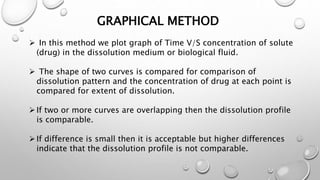
Definition
It is graphical representation in terms of [concentration
vs. time] of complete release of A.P.I. from a dosage form
in an appropriate selected dissolution medium.](https://image.slidesharecdn.com/dissolutionprofilecomparison-180207141108/85/Dissolution-profile-comparison-3-320.jpg)

![STATISTICAL ANALYSIS
1.Student’s t-Test:
The test under the student t-Test are ;
a) One sample t-test
b) Paired t-test
c) Unpaired t-test
The equation for the t is
t = [ X – μ ] / S / √N
Where X is sample mean
N is sample size
S is sample standard deviation
µ is population standard deviations ,](https://image.slidesharecdn.com/dissolutionprofilecomparison-180207141108/85/Dissolution-profile-comparison-9-320.jpg)


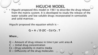


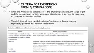
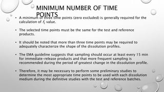
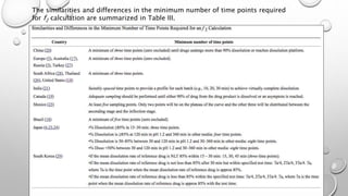


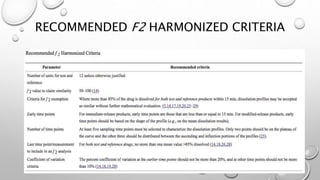


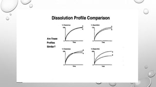
This document compares different methods for comparing dissolution profiles of drug products. It defines dissolution profile comparison and its objectives such as developing bioequivalent products and in vitro-in vivo correlations. Graphical, statistical, model-dependent and model-independent methods are described. The most common model-independent method is the f2 similarity factor test recommended by the FDA, which provides a single value to determine if two dissolution profiles are similar based on the percent dissolved over time. Proper selection of time points and criteria for coefficient of variation are important for f2 testing.


![Rate limiting steps in drug absorption [autosaved]](https://cdn.slidesharecdn.com/ss_thumbnails/ratelimitingstepsindrugabsorptionautosaved-200623174235-thumbnail.jpg?width=640&height=640&fit=bounds)


