5. Περίληψη
Έχουμε πλέον εισέλθει στην εποχή όπου ο όγκος των δεδομένων προς επεξεργασία είναι ασύλληπτα
μεγάλος και τα συστήματα/εφαρμογές που καλούνται να χρησιμοποιήσουν τόσο όγκο πληροφορίας
αδυνατούν, όταν στηρίζονται στις παραδοσιακές μεθόδους. Γι’ αυτό το λόγο, έχουν δημιουργηθεί
πολυπήρηνα συστήματα, σύγχρονες αρχιτεκτονικές υπολογιστών και μέθοδοι παράλληλης επεξεργα-
σίας με στόχο να λύσουν το παραπάνω πρόβλημα με αποδοτικό και γρήγορο τρόπο. Ωστόσο, τα νέα
υπολογιστικά συστήματα και οι τρόποι επεξεργασίας διαθέτουν ένα μεγάλο βαθμό πολυπλοκότητας
στη λειτουργία τους, τον οποίο και μεταφέρουν στην προσαρμογή των εφαρμογών και προγραμμά-
των που χειρίζονται μεγάλους όγκους δεδομένων. Ταυτόχρονα, έχουν δημιουργηθεί όρια απόδοσης
και κατανάλωσης ενέργειας τα οποία είναι απαραίτητο να τηρούνται για την εξοικονόμηση πόρων
και ενέργειας. Μέχρι στιγμής, αυτά τα δύο κομβικά σημεία καλείται να εκτελέσει ο ίδιος ο προγραμ-
ματιστής. Πρέπει να αναλύσει το κάθε πρόγραμμα ανεξάρτητα και να εξετάσει τον τρόπο εκτέλεσής
του μέχρι να βρει την κατάλληλη μορφή που θα τηρεί τους περιορισμούς που έχουν τεθεί. Προφα-
νώς, αυτό το έργο αποτελεί πολύ δύσκολη δουλειά και συνήθως η προσαρμογή προγραμμάτων από
ανθρώπους δεν εξαντλεί όλα τα περιθώρια βελτίωσης. Συνεπώς, καθίσταται απαραίτητη η δημιουρ-
γία ενός εργαλείου που θα αυτοματοποιεί αυτό το έργο και θα παρέχει αποδοτικότερες μορφές των
προγραμμάτων σε μικρό χρονικό διάστημα.
Η παρούσα διπλωματική εργασία παρουσιάζει τον Autotuner, ένα άμεσο και κλιμακωτό εργαλείο που
αναπτύχθηκε ειδικά για την πλατφόρμα Intel Xeon Phi coprocessor και προτείνει, για κάθε εφαρμογή
που δέχεται, περιβάλλοντα διαμόρφωσης για την αποδοτικότερη εκτέλεσή τους στην πλατφόρμα.
Αντικαθιστά έτσι την χειρονακτική δουλεία που έπρεπε να κάνει ο προγραμματιστής καθώς καλού-
νταν να εξερευνήσει 2,880 διαφορετικά περιβάλλοντα εκτέλεσης. Αντί να αναλύει κάθε εφαρμογή
πάνω σ’ όλα τα περιβάλλοντα εκτέλεσης, χρησιμοποιεί πληροφορίες που το εργαλείο έχει αποθηκεύ-
σει από προηγούμενες εφαρμογές. Η λειτουργία του βασίζεται σε μια collaborative filtering μέθοδο
έτσι ώστε γρήγορα και με ακρίβεια να κατηγοροποιεί μια εφαρμογή σε σύνολα περιβάλλοντων εκτέ-
λεσης βρίσκοντας ομοιότητες με προηγούμενες εφαρμογές που έχουν βελτιστοποιηθεί.
Ο Autotuner ελέγθηκε πάνω σε ένα σύνολο απαιτητικών και διαφορετικών εφαρμογών από δύο σύγ-
χρονες σουίτες και οι μετρήσεις ήταν πολύ ενθαρρυντικές. Συγκεριμένα, σε λιγότερο από 8 λεπτά για
κάθε εφαρμογή o Autotuner πρότεινε ένα περιβάλλον διαμόρφωσης που η απόδοσή του ξεπερνούσε
το 90% της καλύτερης εκτέλεσης.
Λέξεις κλειδιά
αυτόματη προσαρμογή, αυτόματη διαμόρφωση, μηχανική μάθηση, Intel Xeon Phi επεξεργαστής, πο-
λυπύρηνα συστήματα, συμβουλευτικό σύστημα, μοντέλο μοιραζόμενης μνήμης, παρακολούθηση, με-
γάλος όγκος δεδομένων.
5
6.
7. Abstract
We have already entered the era where the size of the data that need processing is extremely large and
the applications that use them face difficulties if they follow the traditional ways. For that reason, new
approaches have been developed, multi- and many- core systems, modern computing architectures and
parallel processing models that aim to provide a solution for that problem efficiently and in a timely
manner. However, these new computing systems kai processing methods are characterized by a lot
inner complexity and that complexity is transfered also to programs’ and applications’ tuning which
analyze big data. Concurrently, there have beed set performance and power limitations that need to
comply with. Until now, these two major tasks are tackled by the application developer himself. He has
to analyze every application independently and examine the its execution in order to find the version
that will fulfill the restraints that have been set. Obviously, this is an onerous task and usually hand
tuning does not fully exploit the margins for improvement. Hence, it is crusial the developement of a
tool that will automate program tuning and will provide efficient tuned programs in a small period of
time.
This diploma thesis presents, the Autotuner, an online and scalable tool that was developed specifi-
cally for the Inte Xeon Phi coprocessor and suggests for every incoming application, a performance
effective and energy-saving tuning configuration. It substitutes the hard work the application devel-
oper had to do, as he had to explore 2,880 different tuning configurations. Instead of analyzing every
application against every tuning configuration, it uses previously cached information from already
checked applications. The Autotuner is based on a collaborative filtering technique that quickly and
with accuracy classifies an application with respect to sets of tuning configurations by identifying
similarities to previously optimized applications.
The Autotuner was tested against a set of demanding and diverse applications from two modern bench-
mark suites and the evaluation looked very promising. Particularly, in less than 8 minutes for every
appplication the Autotuner suggested a tuning environment in which the application achieved more
than 90% of the best tuning configuration.
Key words
automatic tuning, machine learning, Intel Xeon Phi coprocessor, manycore systems, multicore sys-
tems, recommender system, shared memory model, monitoring, big data.
7
8.
9. Ευχαριστίες
Η παρούσα διπλωματική εργασία σηματοδοτεί την ολοκλήρωση των σπουδών μου στη σχολή των
Ηλεκτρολόγων Μηχανικών και Μηχανικών Υπολογιστών του Ε.Μ.Π. και κλείνει ένα ταξίδι στο χώρο
των υπολογιστών που αν την πρώτη μέρα φαινόταν ενδιαφέρον σήμερα φαντάζει συναρπαστικό και
μοναδικό. Οι γνώσεις και οι εμπειρίες που απέκτησα με εξέλιξαν σαν άνθρωπο και με βοήθησαν να
αναπτύξω τη δική μου σκέψη ως μηχανικός.
Αρχικά, θα ήθελα να ευχαριστήσω τον επιβλέποντα καθηγητή μου κ. Δημήτριο Σούντρη για την εμπι-
στοσύνη που μου έδειξε, για το θερμό του καλοσώρισμα όταν πρωτοπήγα στο microlab και για την
συνεχή του αμέριστη υποστήριξη. Με βοήθησε να εφαρμόσω την θεωρία στην πράξη και έτσι να έχω
μια πιο πρακτική προσέγγιση αλλά ταυτόχρονα σωστά θεμελιωμένη. Επίσης θα ήθελα να εκφράσω
την ευγνομωσύνη μου τον Δρ. Σωτήρη Ξύδη ο οποίος μου μετέφερε την ιδέα του και μαζί την ανα-
πτύξαμε περισσότερο - θεωρώ προς το καλύτερο - με αποτέλεσμα αυτή την εργασία. Η καθοδήγησή
του καθ’ όλη τη διάρκεια της διπλωματικής μου και η προτροπή του για το κάτι παραπάνω συνέβαλαν
μόνο θετικά στο σύνολο αλλά και σε μένα τον ίδιο.
Τέλος, οφείλω ένα μεγάλο ευχαριστώ στους γονείς μου που ήταν και είναι πάντα δίπλα μου και με
στηρίζουν, καθώς και στα κοντινά μου πρόσωπα και φίλους, παλιούς και νέους, στην Ελλάδα και στο
εξωτερικό, με τους οποίους η συναναστροφή και η ανταλλαγή ιδεών διέρυνε τους ορίζοντες μου και
με έκανε καλύτερο. Η φιλία τους είναι αναντικατάστατη και καθένας και καθεμία έχει σημαδέψει τον
χαρακτήρα μου.
Ελευθέριος - Ιορδάνης Χριστοφορίδης,
Αθήνα, 21η Ιουλίου 2016
9
13. List of Figures
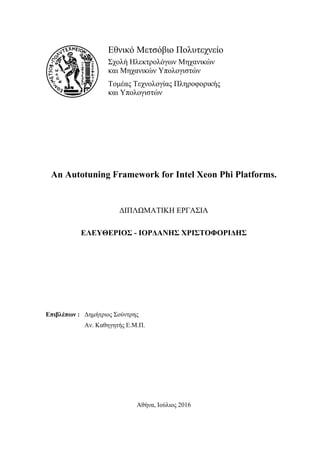
1.1 Performance achieved from predicted configurations in less than 8 minutes profiling. 20
3.1 Overview of the coprocessor silicon and the On-Die Interconnect (ODI)[46]. . . . . 31
3.2 Architecture of a Single Intel Xeon Phi Coprocessor Core[46]. . . . . . . . . . . . . 32
3.3 Roofline model . . . . . . . . . . . . . . . . . . . . . . . . . . . . . . . . . . . . . 37
3.4 Affinity Types (a) Scatter (b) Balanced. . . . . . . . . . . . . . . . . . . . . . . . . 41
3.5 Violin plots for the affinity and cores-threads tuning parameters. . . . . . . . . . . . 47
3.6 Violin plots for the prefetch, unroll and optimization level tuning parameters. . . . . 48
3.7 Violin plots for the huge pages and streaming stores tuning parameters. . . . . . . . 49
3.8 Violin plots for different tuning parameters relative to base configuration. . . . . . . 50
4.1 Fictitious latent factor illustration for users and movies[48]. . . . . . . . . . . . . . . 53
4.2 The first two features from a matrix decomposition of the Netflix Prize data[48]. . . 59
4.3 Two-dimensional graph of the applications, rating MFlops/sec/Watts (Normalized to
the base rating). . . . . . . . . . . . . . . . . . . . . . . . . . . . . . . . . . . . . . 60
4.4 Three-dimensional graph of the applications, rating MFlops/sec/Watts (Normalized
to the base rating). . . . . . . . . . . . . . . . . . . . . . . . . . . . . . . . . . . . . 61
4.5 Two-dimensional graph of the applications, rating IPC/Watts. . . . . . . . . . . . . 63
4.6 Break up of a rating. . . . . . . . . . . . . . . . . . . . . . . . . . . . . . . . . . . 65
4.7 Autotuner’s components. . . . . . . . . . . . . . . . . . . . . . . . . . . . . . . . . 65
5.1 RMSE for a number of features with or without feedback. . . . . . . . . . . . . . . . 68
5.2 Average RMSE for a number of features and training size with or without feedback. . 69
5.3 Normalized ratings of predicted configurations with respect to training size. . . . . . 70
5.4 Performance comparison for 12 features, 2%, 5% and 10% known ratings, with feedback. 71
5.5 RMSE for different number of features, with or without feedback based upon the learn-
ing base 2. . . . . . . . . . . . . . . . . . . . . . . . . . . . . . . . . . . . . . . . . 73
5.6 RMSE for a number of features with or without feedback. . . . . . . . . . . . . . . . 75
5.7 Average RMSE for a number of features and training size with or without feedback. . 76
5.8 Normalized ratings of predicted configurations with respect to training sizes. . . . . 76
5.9 Performance comparison for 9 features, 0.5%, 1%, 2% and 5 % known ratings, without
feedback. . . . . . . . . . . . . . . . . . . . . . . . . . . . . . . . . . . . . . . . . 77
5.10 RMSE for different number of features, with or without feedback based upon the learn-
ing base 2. . . . . . . . . . . . . . . . . . . . . . . . . . . . . . . . . . . . . . . . . 80
5.11 RMSE for different number of features, with or without feedback based upon the learn-
ing base 3. . . . . . . . . . . . . . . . . . . . . . . . . . . . . . . . . . . . . . . . . 81
5.12 RMSE for different number of features, with or without feedback based upon the learn-
ing base by Pearson’s similarity. . . . . . . . . . . . . . . . . . . . . . . . . . . . . 82
5.13 Predicted configurations ratings normalized to the best one with respect to training size. 82
5.14 Performance comparison for 6 features, 0.1%, 0.2% and 5% known ratings, without
feedback. . . . . . . . . . . . . . . . . . . . . . . . . . . . . . . . . . . . . . . . . 83
5.15 Performance vs Time, autotuner without feedback, 0.1% and 2% training sizes . . . 84
5.16 Performance vs Time, autotuner with feedback, 0.1% and 2% training sizes . . . . . 85
13
14.
15. List of Tables
3.1 Coprocessors core’s cache parameters. . . . . . . . . . . . . . . . . . . . . . . . . . 32
3.2 Some hardware events of the coprocessor. . . . . . . . . . . . . . . . . . . . . . . . 34
3.3 Coprocessor’s power consumption on different power states[45]. . . . . . . . . . . . 35
3.4 Summary of tuning parameters. . . . . . . . . . . . . . . . . . . . . . . . . . . . . . 40
3.5 Summary of Rodinia Applications . . . . . . . . . . . . . . . . . . . . . . . . . . . 44
3.6 Summary of NAS benchmarks. . . . . . . . . . . . . . . . . . . . . . . . . . . . . . 46
4.1 Table with the training and test sets from the 2D neighboring. . . . . . . . . . . . . . 61
4.2 Coefficient matrix for all the applications when rated by 1 . . . . . . . . . . . . . . 62
4.3 Table with the training and test sets from the coefficient matrix 4.2. . . . . . . . . . 63
4.4 Table with the training and test sets from the 2D projection 4.5. . . . . . . . . . . . . 63
4.5 Coefficient matrix for all the applications when rated by 2 . . . . . . . . . . . . . . 64
5.1 Learing and regulating rates used. . . . . . . . . . . . . . . . . . . . . . . . . . . . 68
5.2 Correlations between the predicted configurations and the best one by application and
by average for different training sizes. . . . . . . . . . . . . . . . . . . . . . . . . . 70
5.3 Predicted ratings for 12 features, 2%, 5% and 10% known ratings, with feedback along
with the actual and the base ratings. . . . . . . . . . . . . . . . . . . . . . . . . . . 71
5.4 Best configurations both actual and predicted. . . . . . . . . . . . . . . . . . . . . . 72
5.5 Learing and regulating rates used. . . . . . . . . . . . . . . . . . . . . . . . . . . . 74
5.6 Correlations between the predicted configurations and the best one by application and
by average for different training sizes. . . . . . . . . . . . . . . . . . . . . . . . . . 77
5.7 Predicted ratings for 9 features, 5% and 10% known ratings, without feedback along
with the actual and the base ratings. . . . . . . . . . . . . . . . . . . . . . . . . . . 78
5.8 Best configurations both actual and predicted. . . . . . . . . . . . . . . . . . . . . . 79
5.9 Minimum, maximum and average correlations of the 0.1%, 0.2% and 5% predicted
configurations with the best one. . . . . . . . . . . . . . . . . . . . . . . . . . . . . 83
5.10 Percentage change of raw performance between energy aware and unaware predictions. 86
5.11 Best configurations both actual and predicted for energy aware and non-aware ratings. 87
6.1 Average percentages of the predicted configurations from the best and base ratings. . 90
15
16.
17. Chapter 1
Introduction
It is evident that after almost five decades, the end of Moore’s law is in sight. Making transistors
smaller no longer guarantees that they will be faster, power efficient, reliable and cheaper. However,
this does not mean progress in computing has reached its limit, but the nature of that progress is
altered. So, in parallel with the now slower improvement of raw hardware performance, the future of
computing will be primarily defined by improvements in three other areas.
The first one is software. Many examples and very recently AlphaGo[19], have demonstrated that huge
performance gains can be achieved through new algorithms, persevering the current hardware. The
second is the ”cloud”, the networks of data centers that deliver on-line services. By sharing their re-
sources, existing computers can greatly add to their capabilities. Lastly, the third area lies in new com-
puting architectures. Examples are multi- and many-core processors, accelerators(GPGPUs,FPGAs).
These new architectures support also parallelism and they form the High Performance Computing(HPC)
area.
Focusing on the latter, we note that parallel computer systems are getting increasingly complex. The
reasons mainly lie in the exponential upsurge of data to interpret and the far more demanding appli-
cations (e.g. sciences, optimization, simulations). Systems of the past are incapable of processing that
data quickly as the world demands. For these reasons, HPC systems today with a peak performance
of several petaflops have hundreds of thousands of cores that have to be able to work together and
use their resources efficiently. They consist of hardware units that accelerate a specific operation and
they use evolved ideas in data storage, load balancing and intercommunication. Unfortunately, appli-
cations as they were used to run, do not deliver the maximum performance when they are ported on
these systems. As a consequence, high amount of energy and money are being lost because of the low
processor utilization. To reverse that state, programmers need to understood their machine’s unique
architecture and tune their program in a way that exploits every hardware unit optimally. Only then
their program will get the maximum capable throughput.
Besides performance, there is a need to reduce power consumption of those systems. The energy crisis
sets limitations to the amounts of power every system consumes. Towards that goal, a programmer
applies advanced hardware and software techniques (e.g. GPUs, Dynamic Voltage and Frequency
Scaling) which create a trade-off between performance and power saving, thus increasing the difficulty
of the tuning process. By assembling all the choices and the configurations that a programmer has to
weight in order to tune effectively his application, a homogeneous system transforms eventually into
a heterogeneous one, which complicates programming tasks.
However, the tuning process is not at all easy. Application developers are investing significant time to
tune their codes for the current and emerging systems. This tuning can be described as a cyclic process
of gathering data, identifying code regions that can be improved, and tuning those code regions[24].
Alas, this task is toilsome, time-consuming and sometimes practically forbidden to be carried out
manually.
The goal is to automate that task and outperform the human tuning. To accomplish that the research
17
18. community has divided the tuning process into two blocks, performance analysis tools and perfor-
mance autotuning tools. Both the academic and the commercial world have developed tools that
support and partially automate the identification and monitoring of applications[13, 43]. Moreover,
special reference receives the Roofline model[65] which exposes the performance ceilings of an ar-
chitecture along with the position of the application under evaluation, thus providing more accurate
guidance in the tuning procedure.
The tools, until now, do not produce automatically an optimized executable, on the contrary they limit
their operation to characterizations of code regions and simple suggestions to the developer, who man-
ually makes any changes and repeats the tuning phase. As a result much research has been dedicated
during the latest years to automate the tuning phase. Strategies that are employed, have as critical point
to automatically and efficiently search for the best combination of parameter configurations of the ex-
ecution environment for each particular application on a specific architecture. The ideas that have
emerged in the area of automatic tuning have provided encouraging results and have highly benefited
application programmers [52, 60, 38].
A leading example of manycore systems that is used today is Intel Many Integrated Core Architec-
ture (Intel MIC)[4], a coprocessor developed by Intel. The first prototype was launched in 2010 with
the code name Knights Ferry. A year later the Knights Corner product was announced and from
June 2013 the coprocessor is in its second generation Knights Landing. Very soon, along with Intel
Xeon processors-based systems, they became the primary components of supercomputers. Currently,
Tianhe-2(MilkyWay-2) the supercomputer at National Supercomputer Center in Guangzhou, which
holds the first place in the Top500 list[15], is composed of 32,000 Intel Xeon E5-2692 12C at 2.200
GHz and 48,000 Xeon Phi 31S1P, reaching 33,862.7 TFLOP/S. However, many applications have not
yet been structured to take advantage of the full magnitude of parallelism, the high interconnection and
bandwidth rates and the vectorization capabilities of the Intel Xeon Phi. Achieving high performance
with that platform still needs lot of effort on parallelization, analysis and optimization strategies[33].
Hence, investigating and evaluating tuning on a state of the art system, such as Intel Xeon Phi, is
certainly a very valuable and a promising contribution in the areas of HPC and auto-tuning.
18
19. 1.1 Contribution
In this thesis, we develop an auto-tuning framework for Intel Xeon Phi co-processors based on analyt-
ical methods. Its purpose is to relieve the application developer from configuring the compiler and the
execution environment by efficiently and optimally finding the solution that delivers the best outcome
in respect of performance and power.
Shortly, the Autotuner has an offline database of performance data from a set of diverse applica-
tions executed on a set of configurations. These data were collected using LIKWID[62], a lightweight
performance-oriented tool suite for x86 multicore environments. The framework uses these data to
find correlations between the applications and the configurations that are being examined. To achieve
this it uses a collaborative filtering technique[48, 35] that exploits the idea behind Singular Value De-
composition (SVD)[50]. Hence, applications and configurations are mapped to a feature space. That
is a set of attributes, which consists of some configurations, and the scalar relation of the applications
and the configurations to those attributes. Then each new application that arrives, is minimally profiled
to a couple configurations and then it is projected to the constructed feature space, based on its ratings
for the known configurations. Correlations with each feature are produced and consequently, its un-
known ratings can be calculated. In the end, we have a fully populated vector with predicted ratings
for all the configurations, from which we are able to choose the best predicted rating that corresponds
to a specific configuration.
In addition, the auto-tuning framework we developed substantiates the employment of machine learn-
ing techniques and the utilization of their capabilities in the scarce field of autotuners and contributes
significantly to it. Besides the fast predictions and the good performance, singular value decomposition
also reduces the space needed for the characterization of the applications against the configurations,
thus storing huge info in small space.
To have a glance at our results, the Autotuner manages to constantly report a tuning configuration
that achieves more than 90% of the performance that corresponds to the best execution. In addition,
that happens in less than 8 minutes, which is the time for the partial profiling of the application over a
couple tuning configurations. Figure 1.1 shows the performance achieved from the predicted config-
urations for 6 applications.
19
20. Figure 1.1: Performance achieved from predicted configurations in less than 8 minutes profiling.
1.2 Thesis Structure
The thesis is organized as follows:
Chapter 2
We describe performance analysis and tuning tools along with worth noting examples. In addition
some related auto-tuners and their field of application. Lastly, we point out the main differences be-
tween our auto-tuning framework and the rest of the bibliography.
Chapter 3
We describe the system we used, Intel Xeon Phi and the application programming interface (API).
Furthermore we present the Roofline model [reference] for the Intel Xeon Phi. Lastly, we define our
tuning exploration space and we describe the applications used in the evaluation.
Chapter 4
We present meticulously the strategy and the theory behind the Autotuner and its building blocks.
How we extract information while executing an application and how we apply collaborative filtering
for our recommendation system.
20
21. Chapter 5
We demonstrate the experimental results and the efficiency of the Autotuner. We perform an scrupu-
lous evaluation with many varying parameters.
Chapter 6
We briefly conclude and refer to future work.
Appendix A
User manual and source code for the set up of the Autotuner framework.
21
22.
23. Chapter 2
Related Work
2.1 Performance Analysis
Performance analysis tools support the programmer in gathering execution data of an application and
identifying code regions that can be improved. Overall, they monitor a running application. Perfor-
mance data are both summarized and stored as profile data or all details are stored in trace files.
State of the art performance analysis tools fall into two major classes depending on their monitoring
approach:
• profiling tools
• and tracing tools
Profiling tools summarize performance data for the overall execution and provide information such
as the execution time for code regions, number of cache misses, time spent in MPI routines, and
synchronization overhead for OpenMP synchronization constructs.
Tracing tools provide information about individual events, generate typically huge trace files and
provide means to visually analyze those data to identify bottlenecks in the execution.
Representatives for these two classes are Gprof[3], OmpP[36], Vampir[17], PAPI[26], Likwid[62]
and Intel® VTune™Amplifier[43].
2.1.1 Gprof
Gprof is the GNU Profiler tool. It provides a flat profile and a call graph profile for the program’s
functions. Instrumentation code is automatically inserted into the code during compilation, to gather
caller-function data. The flat profile shows how much time the program spent in each function and
how many times that function was called. The call graph shows for each function, which functions
called it, which other functions it called, and how many times. There is also an estimate of how much
time was spent in the subroutines of each function. Lastly there is the annotated source listing which
is a copy of the program’s source code, labeled with the number of times each line of the program
was executed. Yet, Gprof cannot measure time spent in kernel mode (syscalls, waiting for CPU or I/O
waiting) and it is not thread-safe. Typically it only profiles the main thread.
23
24. 2.1.2 OmpP
OmpP is a profiling tool specifically for OpenMP developed at TUM and the University of Tennessee.
It is based on instrumentation with Opari, while it supports the measurement of hardware performance
counters using PAPI. It is capable to expose productivity features such as overhead analysis and detec-
tion of common inefficiency situations and determines certain overhead categories of parallel regions.
2.1.3 Vampir
Vampir is a commercial trace-based performance analysis tool for MPI, from Technische Universität
Dresden. It provides a powerful visualization of traces and scales to thousands of processors based on
a parallel visualization server. It relies on the MPI profiling interface that allows the interception and
replacement of MPI routines by simply re-linking the user-application with the tracing or profiling
library The tool is well-proven and widely used in the high performance computing community for
many years.
2.1.4 PAPI
The Performance API (PAPI) project specifies a standard application programming interface for ac-
cessing hardware performance counters available on most modern microprocessors. Developed at the
University of Tennessee, it provides two interfaces to the underlying counter hardware; a simple, high
level interface for the acquisition of simple measurements and a fully programmable, low level ,inter-
face directed towards users with more sophisticated needs. In addition, it provides portability across
different platforms. It can be used both as a standalone tool and as lower layer of 3rd party tools (ompP,
Vampir etc.)
2.1.5 Intel®
VTune™Amplifier
Intel® VTune™Amplifier is the commercial performance analysis tool of Intel. It provides insight into
CPU and GPU performance, threading performance and scalability, bandwidth, caching, hardware
event sampling etc. In addition, it provides detailed data for each OpenMP region highlights tuning
opportunities.
2.1.6 Likwid
Likwid (Like I knew What I Am Doing) developed at University of Erlangen-Nuremberg, is a set of
command-line utilities that addresses four key problems: Probing the thread and cache topology of
a shared-memory node, enforcing thread-core affinity on a program, measuring performance counter
metrics, and toggling hardware prefetchers. An API for using the performance counting features from
user code is also included.
To the previous list have been added lately PA tools that automate the analysis and improve the scal-
ability of the tools. In addition, automation of the analysis facilitates a lot the application developer’s
task.
These tools are based on the APART Specification Language, a formalization of the performance
problems and the data required to detect them, with aim of supporting automatic performance analysis
for a variety of programming paradigms and architectures.
Some are:
24
25. 2.1.7 Paradyn
Paradyn[11] is a performance measurement tool for parallel and distributed programs from University
of Wisconsin, and it was the first automatic online analysis tool. It is based on a dynamic notion of
performance instrumentation and measurement. Unmodified executable files are placed into execution
and then performance instrumentation is inserted into the application program and modified during
execution. The instrumentation is controlled by the Performance Consultant module, that automati-
cally directs the placement of instrumentation. The Performance Consultant has a well-defined notion
of performance bottlenecks and program structure, so that it can associate bottlenecks with specific
causes and specific parts of a program.
2.1.8 SCALASCA
SCALASCA[13] is an automatic performance analysis tool developed at the German Research School
on Simulation Sciences, the Technische Universität Darmstadt and Forschungszentrum Jülich. It is
based on performance profiles as well as on traces. It supports the performance optimization of par-
allel programs by measuring and analyzing their runtime behavior. The analysis identifies potential
performance bottlenecks - in particular those concerning communication and synchronization - and
offers guidance in exploring their causes.
2.1.9 Periscope
Periscope[39] is an automatic performance analysis tool for highly parallel applications written in
MPI and/or OpenMP developed at Technische Universität München. Unique to Periscope is that it
is an online tool and it works in a distributed fashion. This means that the analysis is done while
the application is executing (online) and by a set of analysis agents, each searching for performance
problems in a subset of the application’s processes (distributed). The properties found by Periscope
point to code regions that might benefit from further tuning.
Many more tools have been developed over the years. We mentioned some examples with particular
interest.
2.2 Performance Autotuning
The core of the tuning process is the search for the optimal combination of code transformations and
parameter settings of the execution environment that satisfy a specific goal. This creates an enormous
search space which further complicates the tuning task. Thus, automation of that step is more than
essential. Much research has been conducted on that matter and as a result many different ideas have
been published. These can be grouped into four categories:
• self-tuning libraries for linear algebra and signal processing like ATLAS, FFTW, OSKI, FEniCS
and SPIRAL;
• tools that automatically analyze alternative compiler optimizations and search for their optimal
combination;
• autotuners that search a space of application-level parameters that are believed to impact the
performance of an application;
• frameworks that try to combine ideas from all the other groups.
25
26. 2.2.1 Self-Tuning libraries
The Automatically Tuned Linear Algebra Software[1] (ATLAS) supports the developers in applying
empirical techniques in order to provide portable performance to numerical programs. It automati-
cally generates and optimizes the popular Basic Linear Algebra Subroutines (BLAS) kernels for the
currently used architecture.
Similarly, FFTW[34] is a library for producing efficient signal processing kernels on different archi-
tectures without modification.
OSKI[9] is a collection of low-level C primitives that provide automatically tuned computational
kernels on sparse matrices, for use in solver libraries and applications.
The FEniCS Project[20] is a collaborative project for the development of innovative concepts and tools
for automated scientific computing, with a particular focus on the solution of differential equations by
finite element methods.
Divergent from the previous, SPIRAL[56] is a program generation system (software that generates
other software) for linear transforms and an increasing list of other mathematical functions. The
goal of Spiral is to automate the development and porting of performance libraries producing high-
performance tuned signal processing kernels.
2.2.2 Compiler optimizations search
This approach is based on the need for more general and application independent auto-tuning. Hence,
the goal is to define the right compiler optimization parameters on any platform. Such tools are divided
into two categories, depending on their strategy.
Iterative search tools iteratively enable certain optimization parameters and run the compiled pro-
gram while monitoring its execution. Following, based on the outcome, they decide on the new
tuning combination. Due to the huge search space, they are relatively slow. In order to tackle
that drawback some algorithms have been built that prune the search space.
Triantafyllis et al[63] as well as Haneda et al[41] enhance that idea by employing heuristics and
statistic methods achieving remarkable results.
Machine Learning tools use knowledge about the program’s behavior and machine learning tech-
niques (e.g. linear regression, support vector machines) to select the optimal combination of
optimization parameters. This approach is based on an automatically build per-system model
which maps performance counters to good optimization options. This model can then be used
with different applications to guide their tuning. Current research work is also targeting the
creation of a self-optimizing compiler that automatically learns the best optimization heuristics
based on the behavior of the underlying platform, as the work of Fursin et al[37] indicates. In
general, machine learning tools explore a much larger space and faster comparing with iterative
search tools.
Ganapathi et al[38], Bergstra et al[25], Leather et al[49] and Cavazos et al[27] are some who
have experimented with machine learning techniques in auto-tuning with auspicious results.
2.2.3 Application parameters search
Somehow more specific, this approach evaluates application’s behavior by exploring its parameters
and implementation. By parameters we refer to global loop transformations (i.e. blocking factor, tiling,
26
27. loop unroll, etc) and by implementation we refer to which algorithms are being used. Thus, this tech-
nique requires in advance some info regarding the application and which parameters should be tuned,
although it is able to get some generality regarding applications with common functions such as matrix
multiplications.
Tools in this category are also divided into two groups. 1. Iterative search tools 2. and Machine learning
tools.
The Intel Software Autotuning tool (ISAT)[51] is an example of iterative search tool which explores
an application’s parameter space which is defined by the user. Yet, it is a time consuming task.
The Active Harmony system[61] is a runtime parameter optimization tool that helps focus on the
application-dependent parameters that are performance critical. The system tries to improve perfor-
mance during a single execution based on the observed historical performance data. It can be used to
tune parameters such as the size of a read-ahead buffer or what algorithm is being used (e.g., heap sort
vs. quick sort).
Focusing on the algorithmic autotuning, Ansel et al[22] developed PetaBricks a new implicitly parallel
programming language for high performance computing. Programs written in PetaBricks can naturally
describe multiple algorithms for solving a problem and how they can be fit together. This information
is used by the PetaBricks compiler and runtime to create and autotune an optimized hybrid algo-
rithm. The PetaBricks system also optimizes and autotunes parameters relating to data distribution,
parallelization, iteration, and accuracy. The knowledge of algorithmic choice allows the PetaBricks
compiler to automatically parallelize programs using the algorithms with the most parallelism.
A different approach followed by Nelson et al[55], interacts with the programmer to get high-level
models of the impact of parameter values. These models are then used by the system to guide the search
for optimization parameters. This approach is called model-guided empirical optimization where mod-
els and empirical techniques are used in a hybrid approach.
Using a totally different method from everything else MATE (Monitoring, Analysis and Tuning
Environment)[53] is an online tuning environment for MPI parallel applications developed by the
Universidad Autònoma de Barcelona. The fundamental idea is that dynamic analysis and online mod-
ifications adapt the application behavior to changing conditions in the execution environment or in
the application itself. MATE automatically instruments at runtime the running application in order
to gather information about the applications behavior. The analysis phase receives events, searches
for bottlenecks by applying a performance model and determines solutions for overcoming such per-
formance bottlenecks. Finally, the application is dynamically tuned by setting appropriate runtime
parameters. All these steps are performed automatically and continuously during application execu-
tion by using the technique called dynamic instrumentation provided by the Dyninst library. MATE
was designed and tested for cluster and grid environments.
2.2.4 Compiler optimizations & Application parameters search
The last category mixes ideas and strategies from both the last two, achieving very positive results.
Some solutions are problem targeted, meaning that they are implemented for specific applications and
some others are more general as they tackle a bigger and more diverse set of applications. Proportion-
ally, their complexity is increasing.
Many autotuning methods have been developed focusing on signal processing applications, matrix
vector multiplication and stencil computations. They take into account both application’s and sys-
tem’s environment parameters. Contributions to this approach come from S. Williams[66] who im-
plements autotuners for two important scientific kernels, Lattice Boltzmann Magnetohydrodynamics
(LBMHD) and sparse matrix-vector multiplication (SpMV). In an automated fashion, these autotuners
27
28. explore the optimization space for the particular computational kernels on an extremely wide range
of architectures. In doing so, it is determined the best combination of algorithm, implementation, and
data structure for the combination of architecture and input data.
As stencil computations are difficult to be assembled into a library because they have a large va-
riety and diverse areas of applications in the heart of many structured grid codes, some autotuning
approaches[31, 47, 30] have been proposed that substantiate the enormous promise for architectural
efficiency, programmer productivity, performance portability, and algorithmic adaptability on exist-
ing and emerging multicore systems.
General autotuners need more information about each application they examine, and for that reason
a performance tool is also needed to reckon the bottlenecks and the critical areas that will deliver
more performance by optimization. Popular examples are Parallel Active Harmony, the Autopilot
framework and the AutoTune project.
The Parallel Active Harmony[60] is a combination of the Harmony system and the CHiLL[29] com-
piler framework. It is an autotuner for scientific codes that applies a search-based autotuning approach.
While monitoring the program performance, the system investigates multiple dynamically generated
versions of the detected hot loop nests. The performance of these code segments is then evaluated in
parallel on the target architecture and the results are processed by a parallel search algorithm. The best
candidate is integrated into the application.
The Autopilot[57] is an integrated toolkit for performance monitoring and dynamical tuning of het-
erogeneous computational grids based on closed loop control. It uses distributed sensors to extract
qualitative and quantitative performance data from the executing applications. This data is processed
by distributed actuators and the preliminary performance benchmark is reported to the application
developer.
AutoTune project[52] extends Periscope with plugins for performance and energy efficiency tuning,
and constitutes a part of the Periscope Tuning Framework (PTF)[39]. PTF supports tuning of appli-
cations at design time. The most important novelty of PTF is the close integration of performance
analysis and tuning. It enables the plugins to gather detailed performance information during the eval-
uation of tuning scenarios to shrink the search space and to increase the efficiency of the tuning plugins.
The performance analysis determines information about the execution of an application in the form
of performance properties. The HPC tuning plugins that implemet PTF are: Compliler Flags Selec-
tion Tuning, MPI Tuning, Energy Tuning, Tuning Master Worker Application and Tuning Pipeline
Applications.
An ongoing tuning project is X-TUNE[18] which evaluates ideas to refine the search space and search
approach for autotuning. Its goal is to seamlessly integrate programmer-directed and compiler-directed
auto-tuning, so that a programmer and the compiler system can work collaboratively to tune a code,
unlike previous systems that place the entire tuning burden on either programmer or compiler.
Readex project[12] is another current project which aims to develop a tools-aided methodology for
dynamic autotuning for performance and energy efficiency. The project brings together experts from
two ends of the compute spectrum: the system scenario methodology[40] from the embedded systems
domain as well as the High Performance Computing community with the Periscope Tuning Frame-
work (PTF).
2.3 Autotuners tested on Intel Xeon Phi
Many researchers have been experimenting on the coprocessor developed by Intel to establish a work-
ing and useful autotuner. Intel Xeon Phi coprocessor is interesting among the HPC community because
28
29. of its simple programming model and its highly parallel architecture. Hence, there is a trend to derive
its maximum computational power through fine automatic tuning.
Wai Teng Tang et al[59] implemented sparse matrix vector multiplication (SpMV), a popular kernel
among many HPC applications that use scale-free sparse matrices (e.g. fluid dynamics, social net-
work analysis and data mining), on the Intel Xeon Phi Architecture and optimized its performance.
Their kernel makes use of a vector format that is designed for efficient vector processing and load bal-
ancing. Furthermore, they employed a 2D jagged partitioning method together with tiling in order to
improve the cache locality and reduce the overhead of expensive gather and scatter operations. They
also employed efficient prefix sum computations using SIMD and masked operations that are spe-
cially supported by the Xeon Phi hardware. The optimal panel number in the 2D jagged partitioning
method varies for different matrices due to their differences in non-zero distribution, hence a tuning
tool was developed. Their experiments indicated that the SpMV implementation achieves an aver-
age 3x speedup over Intel MKL for scale-free matrices, and the performance tuning method achieves
within 10 % of the optimal configuration.
Williams et al[64] explored the optimization of geometric multigrid (MG) - one of the most important
algorithms for computational scientists - on a variety of leading multi- and manycore architectural
designs, including Intel Xeon Phi. They optimized and analyzed all the required components within an
entire multigrid V-cycle using a variable coefficient, Red-Black, Gauss-Seidel (GSRB) relaxation on
these advanced platforms. They also implemented a number of effective optimizations geared toward
bandwidth-constrained, wide-SIMD, manycore architectures including the application of wavefront
to variable-coefficient, Gauss-Seidel, Red-Black (GSRB), SIMDization within the GSRB relaxation,
and intelligent communication-avoiding techniques that reduce DRAM traffic. They also explored
message aggregation, residual restriction fusion, nested parallelism, as well as CPUand KNC-specific
tuning strategies. Overall results showed a significant performance improvement of up to 3.8x on
the Intel Xeon Phi compared with the parallel reference implementation, by combining autotuned
threading, wavefront, hand-tuned prefetching, SIMD vectorization, array padding and the use of 2MB
pages.
Heirman et al[42] extent ClusteR - aware Undersubscribed Scheduling of Threads (CRUST), a varia-
tion on dynamic concurrency throttling (DCT) specialized for clustered last-level cache architectures,
to incorporate the effects of simultaneous multithreading, which in addition to competition for cache
capacity, exhibits additional effects incurred by core resource sharing. They implemented this im-
proved version of CRUST inside the Intel OpenMP runtime library and explored its performance
when running on Xeon Phi hardware. Finally, CRUST can be integrated easily into the OpenMP run-
time library; by combining application phase behavior and leveraging hardware performance counter
information it is able to reach the best static thread count for most applications and can even outper-
form static tuning on more complex applications where the optimum thread count varies throughout
the application.
Sclocco et al[58] designed and developed a many-core dedispersion algorithm, and implemented it us-
ing the Open Computing Language (OpenCL). Because of its low arithmetic intensity, they designed
the algorithm in a way that exposes the parameters controlling the amount of parallelism and possi-
ble data-reuse. They showed how, by auto-tuning these user-controlled parameters, it is possible to
achieve high performance on different many-core accelerators, including one AMD GPU (HD7970),
three NVIDIA GPUs (GTX 680, K20 and GTX Titan) and the Intel Xeon Phi. they not only auto-tuned
the algorithm for different accelerators, but also used auto-tuning to adapt the algorithm to different
observational configurations.
ppOpen-HPC[54] is an open source infrastructure for development and execution of large-scale scien-
tific applications on post-peta-scale (pp) supercomputers with automatic tuning (AT). ppOpen-HPC
focuses on parallel computers based on many-core architectures and consists of various types of li-
braries covering general procedures for scientific computations. The source code, developed on a PC
29
30. with a single processor, is linked with these libraries, and the parallel code generated is optimized
for post-peta-scale systems. Specifically on the Intel Xeon Phi coprocessor, the performance of a par-
allel 3D finite-difference method (FDM) simulation of seismic wave propagation was evaluated by
using a standard parallel finite-difference method (FDM) library (ppOpen-APPL/FDM) as part of the
ppOpen-HPC project.
2.4 How our work is different from the bibliography?
The autotuning framework we developed is based on data mining. The autotuner derives its sugges-
tions from an already known set of profiled applications against the full set of configuration space.
Thus, it is sensitive on the choice of those applications that constitute its initial knowledge. It belongs
in the category of machine learning autotuners like Ganapathi[38]. It explores mainly compiler and
execution environment parameters because the configuration space of the coprocessor is large enough.
There is not a specified target group of applications to autotune. It performs well independently of the
current testing application that is why it is a general autotuner.
From our experience with this framework and the employment of data mining techniques, we conclude
that valuable knowledge and fine tuning can be derived from their use and at the same time in timely
fashion with high accuracy. We know the optimal tuning of many applications, we need only to project
them to newly machine architectures in a way to benefit from their capabilities and specifications.
Then it is able to find correlations between them and unoptimized applications in order to suggest the
optimal tuning.
The idea to use data mining techniques in autotuning for a heterogeneous - because of its vary con-
figurations - coprocessor came from the work of Delimitrou and Kozyrakis[32] who developed an
heterogeneity- and interference-aware scheduler, Paragon, for large-scale datacenters. Paragon is an
online and scalable scheduler based on collaborative filtering techniques to quickly and accurately
classify an unknown incoming workload with respect to heterogeneity and interference in multiple
shared resources.
30
31. Chapter 3
Experimental Testbed & Environment
3.1 Intel Xeon Phi
3.1.1 Architecture
In this work we used an Intel®Xeon Phi™coprocessor of the 3100 Series with code name Knights
Corner. It is Intel’s first many-cores commercial product made at a 22nm process size that uses Intel’s
Many Integrated Core (MIC) architecture. A coprocessor needs to be connected to a Host CPU, via
the PCI Express bus and in that way they share access to main memory with other processors.
The coprocessor is a symmetric multiprocessor (SMP) on-a-chip running Linux. It consists of 57 cores
who are in-order dual issue x86 processor cores, they support 64-bit execution environment-based
on Intel64 Architecture and are clocked at 1.1GHz. Each one has four hardware threads, resulting
in 228 available hardware threads. They are used mainly to hide latencies implicit to the in-order
microarchitecture. In addition to the cores, the coprocessor has six memory controllers supporting
two GDDR5 (high speed) memory channels each at 5GT/sec. Each memory transaction to the total
6GB GDDR5 memory is 4 bytes of data resulting in 5GT/s x 4 or 20GB/s per channel. 12 total channels
provide maximum transfer rate of 240GB/s. Then it consists of other device interfaces including the
PCI Express system interface.
All the cores, the memory controllers, and PCI Express system I/O logic are interconnected with a high
speed ring-based bidirectional on-die interconnect (ODI), as shown in Figure 3.1. Communication
over the ODI is transparent to the running code with transactions managed solely by the hardware.
Figure 3.1: Overview of the coprocessor silicon and the On-Die Interconnect (ODI)[46].
31
32. At the core level, exclusives 32-KB L1 instruction cache and L1 data cache as well as a 512-KB Level
2 (L2) are assigned to provide high speed, reusable data access. In Table 3.1 we are summarized the
main properties of the L1 and L2 caches.
Parameter L1 L2
Coherence MESI MESI
Size 32 KB + 32 KB 512 KB
Associativity 8-way 8-way
Line size 64 Bytes 64 Bytes
Banks 8 8
Access Time 1 cycle 11 cycles
Policy Pseudo LRU Pseudo LRU
Table 3.1: Coprocessors core’s cache parameters.
Furthermore, fast access to data in another core’s cache over the ODI is provided to improve perfor-
mance when the data already resides “on chip.” Using a distributed Tag Directory (TD) mechanism,
the cache accesses are kept “coherent” such that any cached data referenced remains consistent across
all cores without software intervention. There are two primary instruction processing units. The scalar
unit executes code using existing traditional x86 and x87 instructions and registers. The vector pro-
cessing unit (VPU) executes the Intel Initial Many Core Instructions (IMCI) utilizing a 512-bit wide
vector length enabling very high computational throughput for both single and double precision cal-
culations. Along there is an Extended Math Unit (EMU) for high performance key transcendental
functions, such as reciprocal, square root, power and exponent functions. The microarchitectural dia-
gram of a core is shown in the Figure 3.2.
Figure 3.2: Architecture of a Single Intel Xeon Phi Coprocessor Core[46].
Each core’s instruction pipeline has an in-order superscalar architecture. It can execute two instruc-
tions per clock cycle, one on the U-pipe and one on the V-pipe. The V-pipe cannot execute all instruc-
tion types, and simultaneous execution is governed by instruction pairing rules. Vector instructions are
mainly executed only on the U-pipe. The instruction decoder is designed as a two-cycle fully pipelined
unit, which greatly simplifies the core design allowing for higher cycle rate than otherwise could be
implemented. The result is that any given hardware thread that is scheduled back-to-back will stall in
decode for one cycle. Therefore, single-threaded code will only achieve a maximum of 50% utilization
32
33. of the core’s computational potential. However, if additional hardware thread contexts are utilized, a
different thread’s instruction may be scheduled each cycle and full core computational throughput
of the coprocessor can be realized. Therefore, to maximize the coprocessor silicon’s utilization for
compute-intensive application sequences, at least two hardware thread contexts should be run.
The coprocessor silicon supports virtual memory management with 4 KB (standard), 64 KB (not
standard), and 2 MB (huge and standard) page sizes available and includes Translation Lookaside
Buffer (TLB) page table entry cache management to speed physical to virtual address lookup as in
other Intel architecture microprocessors.
The Intel Xeon Phi coprocessor includes memory prefetching support to maximize the availability
of data to the computation units of the cores. Prefetching is a request to the coprocessor’s cache and
memory access subsystem to look ahead and begin the relative slow process of bringing data we expect
to use in the near future into the much faster to access L1 and/or L2 caches. The coprocessor provides
two kinds of prefetch support, software and hardware prefetching. Software prefetching is provided
in the coprocessor VPU instruction set. The processing impact of the prefetch requests can be reduced
or eliminated because the prefetch instructions can be paired on the V-pipe in the same cycle with
a vector computation instruction. The hardware prefetching (HWP) is implemented in the core’s L2
cache control logic section.
3.1.2 Performance Monitoring Units
In order to monitor hardware events, the coprocessor is supported by a performance monitoring unit
(PMU). Each physical Intel Xeon Phi coprocessor core has an independent-programmable core PMU
with two performance counters and two event select registers, thus it supports performance monitoring
at the individual thread level. User-space applications are allowed to interface with and use the PMU
features via specialized instructions such as RDMSR, WRMSR, RDTSC, RDPMC. Coprocessor-
centric events are able to measure memory controller events, vector processing unit utilization and
statistics, local and remote cache read/write statistics, and more[44]. In Table 3.2, are shown some
important hardware events of the coprocessor. The rest can be found on [2].
3.1.3 Power Management
Unlike the multicore family of Intel Xeon processors, there is no hardware-level power control unit
in the coprocessor. Instead power management (PM) is controlled by the coprocessor’s operating
system and is performed in the background. Intel Xeon Phi coprocessor power management software
is organized into two major blocks. One is integrated into the coprocessor OS running locally on
the coprocessor hardware. The other is part of the host driver running on the host. Each contributes
uniquely to the overall PM solution.
The power management infrastructure collects the necessary data to select performance states and
target idle states for the individual cores and the whole system. Below, we describe these power
states[44, 45]:
Coprocessor in C0 state; Memory in M0 state In this power state, the coprocessor (cores and
memory) is expected to operate at its maximum thermal design power (TDP), for our coprocessor that
is 300 Watts. While in that state, all cores are active and run at the same P-state, or performance state.
P-states are different frequency settings that the OS or the applications can request. Each frequency
setting of the coprocessor requires a specific voltage identification (VID) voltage setting in order to
guarantee proper operation, thus each P-state corresponds to one of these frequency and voltage pairs.
33
34. Event Description
CPU_CLK_UNHALTED The number of cycles (commonly known as clock-
ticks) where any thread on a core is active. A core
is active if any thread on that core is not halted.
This event is counted at the core level at any given
time, all the hardware threads running on the same
core will have the same value.
INSTRUCTIONS_EXECUTED Counts the number of instructions executed by a
hardware thread.
DATA_CACHE_LINES_WRITTEN_BACK Number of dirty lines (all) that are written back,
regardless of the cause.
L2_DATA_READ_MISS_MEM_FILL Counts data loads that missed the local L2 cache,
and were serviced from memory (on the same In-
tel Xeon Phi coprocessor). This event counts at the
hardware thread level. It includes L2 prefetches
that missed the local L2 cache and so is not use-
ful for determining demand cache fills or standard
metrics like L2 Hit/Miss Rate.
L2_DATA_WRITE_MISS_MEM_FILL Counts data Reads for Ownership (due to a store
operation) that missed the local L2 cache, and
were serviced from memory (on the same Intel
Xeon Phi coprocessor). This event counts at the
hardware thread level.
Table 3.2: Some hardware events of the coprocessor.
P1 is the highest P-state setting and it can have multiple sequentially lower frequency settings referred
as P2,P3,…,Pn where Pn is the lowest pair.
Some cores are in C0 state and other cores in C1 state; Memory in M0 state When all four
threads in a core have halted, the clock at the core shuts off, changing his state to C1. The last thread
to halt is responsible to collect idle residency data and store it in a data structure accessible to the
OS. A coprocessor can have some cores in C0 state and some in C1 state with memory in M0 state.
In this case, clocks are gated on a core-by-core basis, reducing core power and allowing the cores
in C1 state to lose clock source. After a core drops in C1 state, there is the option the core shuts
down, become electrically isolated. That is the core C6 state and it is decided by the coprocessor’s
PM SW, which also writes to a certain status register the current core’s status before issuing HALT to
all the threads active on that core. The memory clock can be fully stopped to reduce memory power
and memory subsystem enters M3 state. The price of dropping into a deeper core C state is an added
latency resulting from bringing the core back up to the non-idle state, so the OS evaluates if the power-
savings are worthwhile.
The coprocessor in package Auto-C3 state; Memory in M1 state If all the cores enter C1 state,
the coprocessor automatically enters auto-package C3 (PC3) state by clock gating also the uncore part
of the card. For this transition both the coprossesor’s PM software and the host’s coprocessor PM
are involved, that is because it may be needed a core to return to C0 state and in order to happen the
coprossesor PM SW must initiate it. In addition, the host’s coprocessors PM may override the request
to PC3 under certain conditions, such as when the host knows that the uncore part of the coprocessor
is still busy. Finally, the clock source to the memory can be gated off also, thus reducing memory
34
35. power. This is the M1 state for the memory.
The coprocessor in package Deep-C3; Memory in M2 state In this state only the host’s copro-
cessor PM SW functions and decides for the transitions as it has a broader sense of the events on
the coprocessor and the coprocessor’s PM SW is essential suspended for the power savings. So the
host’s coprocessor PM SW looks at idle residency history, interrupts (such as PCI Express traffic),
and the cost of waking the coprocessor up from package Deep-C3 to decide whether to transition from
package Auto-C3 state into package Deep-C3 state. In package Deep-C3 the core voltage is further
reduced and the voltage regulators (VRs) enter low power mode. The memory changes to self-refresh
mode, i.e. M2 state.
The coprocessor in package C6; Memory in M3 state The transition to this state can be initiated
from both the coprocessor and the host. More reductions in power consumption are done in the uncore
part, the cores are shut off and the memory clock can be fully stopped, reducing memory power to its
minimum state (M3).
The Table 3.3 shows the power consumed in each state.
Coprocessor’s Power State Power(Watts)
C0 300
C1 <115
PC3 <50
PC6 <30
Table 3.3: Coprocessor’s power consumption on different power states[45].
3.2 Roofline Model
The roofline model is a visual performance model that offers insights to programmers on improving
parallel software for floating point computations relatively to the specifications of the architecture used
or defined by the user. Proposed by Williams et al [65], it has been used and proved valuable both to
guide manual code optimization and in education. Therefore, creating the roofline for our testbed will
aid us in the characterization of the autotuning process, how exactly the unoptimized and optimized
benchmarks move in the 2D space. Firstly, we describe the roofline model and its background.
3.2.1 Model’s Background
The platform’s peak computational performance - generally floating operations - together with the
peak memory bandwidth - generally between the CPU and the main memory - create a performance
”ceiling” in the 2 dimensional space. These peak values are calculated from the hardware specifi-
cations. On the x-axis is the operational intensity, which is defined as the amount of floating points
operations per byte of main memory traffic. On the y-axis is the performance. Both axis are in log
scale. The roofline is visually constructed by one horizontal and one diagonal line. The horizontal line
is the peak performance and the diagonal is the performance limited by memory bandwidth. Thus, the
mathematical equation is:
Roofline(op. intensity) = min(BW * op. intensity, peak performance)
35
36. The point where the two lines intersect:
Peak Performance = Operational Intensity * Memory Bandwidth
is called ridge point and defines the minimum operational intensity that is required in order to reach
maximum computational performance. In addition, the area on the right of the ridge point is called
computational bound and on the left memory bound.
Besides using the peak values calculated from the architecture, one can create a roofline using soft-
ware peak values (lower than the ones from hardware) such as performance limited to thread level
parallelism , instruction level parallelism and SIMD, without memory optimizations (e.g. prefetches,
affinity). In addition, more realistic performance ceilings can be obtained by running standard bench-
marks such as the high-performance LINPACK[8] and the Stream Triad[14] benchmarks. We assume
that any real world application’s performance can be characterized somewhere between totally mem-
ory bandwidth bound (represented by Stream Triad) and totally compute or Flop/s bound (represented
by Linpack).
For a given kernel, we can find a point on the x-axis based on its operation intensity. A vertical
line from that point to the roofline shows what performance is able to achieve for that operational
intensity[65]. From the definition of the ridge point, if the operational intensity of the kernel is on
the left of the ridge point then the kernel is bound from the bandwidth performance and if it is on
the right then the kernel is bound from the peak computational performance. So, by plotting along
with the peak performances also the performances from the software tunings, it can be reckoned what
optimizations will benefit the most the kernel under examination, guide in other words the developer
for the optimum tuning appropriately.
3.2.2 The Roofline of our Testbed
As we noted before, our testbed consists of one Intel Xeon Phi coprocessor 3120A. From the technical
specifications we can calculate the theoretical peak computational performance. With 57 cores, each
running at maximum 1.1GHz, a 512-bit wide VPU unit and support of the instruction fused multiply
and add (FMA) enabling two floating point operations in one instruction, the peak computational
performance is obtained from the formula:
Clock Frequency × Number of Cores × 16 lanes(SP floats) × 2(FMA) FLOPs/cycle
So, by substituting the technical specification values we get: 2006.4 GFlops/sec for SP and 1003.2
GFlops/sec for DP, which is usually the reported one. The theoretical bandwidth between the CPU
and the main memory is 240GB/sec.
By running the standard performance benchmarks with the appropriate optimizations, we get from
Linpack 727.99111 GFlops/sec (DP) and from Stream triad we get 128.312 GB/sec. Both values are
very close to the ones reported by Intel using the same benchmarks[6]. The choice of these two bench-
marks provides a strong hypothesis and we may argue that even if they remain far from ideal reference
points, they represent a better approximation than the hardware theoretical peaks because they at least
include the minimum overhead required to execute an instruction stream on the processing device[21].
1
The performance reported was achieved with the following configuration: compact affinity, 228 threads, size=24592,
ld=24616, 4KB align. The optimized benchmark from the Intel was used[5]
2
The performance reported was achieved with the following configurations as they are suggested here[10]: 110M ele-
ments per array, prefetch distance=64,8, streaming cache evict=0, streaming stores=always, 57 threads, balanced affinity.
36
37. So, now we can compute the operational intensity (OI) of the ridge point for both the theoretical and
the achievable peak performances, as: (using double precision)
OIth
R =
1003.2
240
= 4.18Flops/Byte
OIac
R =
727.9911
128.31
= 5.67Flops/Byte
Figure 3.3 shows the roofline model for our testbed in double precision.
Figure 3.3: Roofline model
3.3 Tuning Parameters
In this section, we describe the parameters we used to build our tuning space. It is composed of com-
piler’s flags as well as environmental configurations for the tuning of each application. The compiler
is the system’s default, Intel®C Intel®64 Compiler XE for applications running on Intel®64, Version
14.0.3.174 (icc).
3.3.1 Compiler’s Flags
The compiler’s flags used where chosen from the icc’s optimization category.
-O[=n]
Specifies the code optimization for applications.
Arguments:
37
38. O2: Enables optimizations for speed. Vectorization is enabled at O2 and higher levels. Some basic
loop optimizations such as Distribution, Predicate Opt, Interchange, multi-versioning, and scalar
replacements are performed. More detailed information can be found on [16].
O3: Performs O2 optimizations and enables more aggressive loop transformations such as Fusion,
Block-Unroll-and-Jam, and collapsing IF statements. The O3 optimizations may not cause higher
performance unless loop and memory access transformations take place. The optimizations may
slow down code in some cases compared to O2 optimizations.
-opt-prefetch[=n]
This option enables or disables prefetch insertion optimization. The goal of prefetching is to reduce
cache misses by providing hints to the processor about when data should be loaded into the cache.
Arguments:
0: Disables software prefetching.
2-4: Enables different levels of software prefetching.
Prefetching is an important topic to consider regardless of what coding method we use to write an
algorithm. To avoid having a vector load operation request data that is not in cache, we can make sure
prefetch operations are happening. Any time a load requests data not in the L1 cache, a delay occurs
to fetch the data from an L2 cache. If data is not in any L2 cache, an even longer delay occurs to fetch
data from memory. The lengths of these delays are nontrivial, and avoiding the delays can greatly
enhance the performance of an application.
-opt-streaming-stores [keyword]
This option enables generation of streaming stores for optimization. This method stores data with
instructions that use a non-temporal buffer, which minimizes memory hierarchy pollution.
Arguments:
never: Disables generation of streaming stores for optimization. Normal stores are performed.
always: Enables generation of streaming stores for optimization. The compiler optimizes under the as-
sumption that the application is memory bound.
Streaming stores are a special consideration in vectorization. Streaming stores are instructions espe-
cially designed for a continuous stream of output data that fills in a section of memory with no gaps
between data items. An interesting property of an output stream is that the result in memory does not
require knowledge of the prior memory content. This means that the original data does not need to
be fetched from memory. This is the problem that streaming stores solve - the ability to output a data
stream but not use memory bandwidth to read data needlessly. Having the compiler generate stream-
ing stores can improve performance by not having the coprocessor fetch caches lines from memory
that will be completely overwritten. This effectively avoids wasted prefetching efforts and eventually
helps with memory bandwidth utilization.
38
39. -opt-streaming-cache-evict[=n]
This option specifies the cache eviction (clevict) level to be used by the compiler for streaming loads
and stores. Depending on the level used, the compiler will generate clevict0 and/or clevict1 instruc-
tions that evict the cache-line (corresponding to the load or the store) from the first-level and second-
level caches. These cache eviction instructions will be generated after performing the corresponding
load/store operation.
Arguments:
0: Tells the compiler to use no cache eviction level.
1: Tells the compiler to use the L1 cache eviction level.
2: Tells the compiler to use the L2 cache eviction level.
3: Tells the compiler to use the L1 and L2 cache eviction level.
-unroll[=n]
This option tells the compiler the maximum number of times to unroll loops.
Arguments:
0: Disables loop unrolling.
N/A: With unspecified n, the optimizer determines how many times loops can be unrolled.
The Intel C Compiler can typically generate efficient vectorized code if a loop structure is not manually
unrolled. Unrolling means duplicating the loop body as many times as needed to operate on data using
full vectors. For single precision on Intel Xeon Phi coprocessors, this commonly means unrolling 16-
times. In other words, the loop body would do 16 iterations at once and the loop itself would need to
skip ahead 16 per iteration of the new loop.
3.3.2 Huge Pages
To get good performance for executions on the coprocessor, huge memory pages (2MB) are often
necessary for memory allocations on the coprocessor. This is because large variables and buffers are
sometimes handled more efficiently with 2MB vs 4KB pages. With 2MB pages, TLB misses and page
faults may be reduced, and there is a lower allocation cost.
In order to enable 2MB pages for applications running on the coprocessor we can either manually
instrument the program with mmap system calls or use the hugetlbfs library[7]. In our case, we used
the hugetlbfs library dynamically linked with the applications.
Although, Manycore Platform Software Stack(MPSS) versions later than 2.1.4982-15 support “Trans-
parent Huge Pages (THP)” which automatically promotes 4K pages to 2MB pages for stack and heap
allocated data, we use the hugetlbfs library to allocate data directly in 2MB pages. This is useful be-
cause if the data access pattern is such that the program can still benefit from allocating data in 2MB
pages even though THP may not get triggered in the uOS.
So, we examined the performance of the applications with huge pages enable or not.
39
40. 3.3.3 OpenMP Thread Affinity Control
Threading and Thread placement
As a minimum number of threads per physical core we set 2 because of the two-cycle fully pipelined
instruction decoder as we mentioned in the coprocessor’s architecture. We examine the performance of
each application on 19, 38 and 57 physical cores and with the different combinations of enabled threads
per core we get 38, 57, 76, 114, 152, 171 and 228 threads with different however mappings on the cores.
That is implemented by using the environmental variable KMP_PLACE_THREADS=ccC,ttT,ooO,
where:
C: denotes the number of physical cores
T: denotes the number of threads per core
O: denotes the offset of cores
So, with this variable we specify the topology of the system to the OpenMP runtime.
Affinity
In order to specify how the threads are bound within the topology we use the environmental variable
KMP_AFFINITY[=type], where type:
scatter: The threads are distributed as evenly as possible across the entire system. OpenMP thread num-
bers with close numerical proximity are on different cores.
balanced: The threads are distributed as evenly as possible across the entire system while ensuring the
OpenMP thread numbers are close to each other.
Below, the Figure 3.4 illustrates the two different affinity types. We note that both types use cores be-
fore threads, thus they gain from every available core. In addition, while in balanced thread allocation
cache utilization should be efficient if the neighbor threads access data that is near in store. Generally
however, tuning affinity is a complicated and machine specific process.
In the Table 3.4 we present a summary of the tuning parameters with their possible values. The total
combinations are 2880 tuning states.
Flag Arguments
-O[=n] n=2,3
-opt-prefetch[=n] n=0,2,3,4
-opt-streaming-stores [keyword] keyword=never,always
-opt-streaming-cache-evict[=n] m=0,1,2,3
-unroll enabled/disabled
huge pages enabled/disabled
affinity [type] type=scatter,balanced
cores 19,38,57
threads per core 2,3,4
Table 3.4: Summary of tuning parameters.
40
41. (a)
(b)
Figure 3.4: Affinity Types (a) Scatter (b) Balanced.
3.4 Applications Used
In order to build and evaluate our autotuner for the coprocessor we used applications from two bench-
marks suites, the Rodinia Benchmark Suite[28] and the NAS Parallel Benchmarks[23]. We focused
only on applications with floating point operations and profiled them against the previous tuning states.
We used the OpenMP implementations.
3.4.1 Rodinia Benchmarks Suite
Rodinia is a benchmark suite for heterogeneous computing. It includes applications and kernels which
target multi- and manycore CPU and GPU platforms. The choice of applications is inspired by Berke-
ley’s dwarf taxonomy. It has been shown[28] that Rodinia covers a wide range of parallel commu-
nication patterns, synchronization techniques and power consumption and has led to some important
architectural insight, such as the growing importance of memory bandwidth limitations and the con-
sequent importance of data layout.
Below we list the applications and kernels we used along with some specifications.
41
42. LU Decomposition(LUD)
LU Decomposition is an algorithm to calculate the solutions of a set of linear equations. The LUD
kernel decomposes a matrix as the product of a lower triangular matrix and an upper triangular ma-
trix. This application has many row-wise and column-wise interdependencies and requires significant
optimization to achieve good parallel performance. The size of the matrix was 8000x8000.
Hotspot
Hotspot is a thermal simulation tool used for estimating processor temperature based on an architec-
tural floor plan and simulated power measurements. It includes the 2D transient thermal simulation
kernel of HotSpot, which iteratively solves a series of differential equations for block temperatures.
The inputs to the program are power and initial temperatures. Each output cell in the grid represents
the average temperature value of the corresponding area of the chip. There is also a 3 dimensional
implementation of the same application. For the standard version we used arrays with 1024x1024
elements for the temperature and the power.
Streamcluster
Streamcluster solves the online clustering problem. For a stream of input points, it finds a pre-determined
number of medians so that each point is assigned to its nearest center. The quality of the clustering is
measured by the sum of squared distances (SSQ) metric. The original code is from the Parsec Bench-
mark suite developed by Princeton University. We used 32768 data points per block and 1 block.
K-means
K-means is a clustering algorithm used extensively in data mining. This identifies related points by
associating each data point with its nearest cluster, computing new cluster centroids, and iterating until
convergence. We used 494020 objects with 34 attributes each.
LavaMD
The code calculates particle potential and relocation due to mutual forces between particles within
a large 3D space. This space is divided into cubes, or large boxes, that are allocated to individual
cluster nodes. The large box at each node is further divided into cubes, called boxes. 26 neighbor
boxes surround each box (the home box). Home boxes at the boundaries of the particle space have
fewer neighbors. Particles only interact with those other particles that are within a cutoff radius since
ones at larger distances exert negligible forces. Thus the box size is chosen so that cutoff radius does
not span beyond any neighbor box for any particle in a home box, thus limiting the reference space
to a finite number of boxes. The space examined was divided into 8000 cubes each with dimensions
20x20x20.
Heartwall
The Heart Wall application tracks the movement of a mouse heart over a sequence of 30 (maximum
104) 744x656 ultrasound images to record response to the stimulus. In its initial stage, the program
performs image processing operations on the first image to detect initial, partial shapes of inner and
42
43. outer heart walls. These operations include: edge detection, SRAD despeckling, morphological trans-
formation and dilation. In order to reconstruct approximated full shapes of heart walls, the program
generates ellipses that are superimposed over the image and sampled to mark points on the heart walls
(Hough Search). In its final stage, program tracks movement of surfaces by detecting the movement
of image areas under sample points as the shapes of the heart walls change throughout the sequence
of images.
Myocyte
Myocyte application models cardiac myocyte (heart muscle cell) and simulates its behavior. The
model integrates cardiac myocyte electrical activity with the calcineurin pathway, which is a key
aspect of the development of heart failure. The model spans large number of temporal scales to reflect
how changes in heart rate as observed during exercise or stress contribute to calcineurin pathway acti-
vation, which ultimately leads to the expression of numerous genes that remodel the heart’s structure.
It can be used to identify potential therapeutic targets that may be useful for the treatment of heart
failure. Biochemical reactions, ion transport and electrical activity in the cell are modeled with 91 or-
dinary differential equations (ODEs) that are determined by more than 200 experimentally validated
parameters. The model is simulated by solving this group of ODEs for a specified time interval. The
process of ODE solving is based on the causal relationship between values of ODEs at different time
steps, thus it is mostly sequential. At every dynamically determined time step, the solver evaluates
the model consisting of a set of 91 ODEs and 480 supporting equations to determine behavior of the
system at that particular time instance. If evaluation results are not within the expected tolerance at
a given time step (usually as a result of incorrect determination of the time step), another calculation
attempt is made at a modified (usually reduced) time step. Since the ODEs are stiff (exhibit fast rate
of change within short time intervals), they need to be simulated at small time scales with an adaptive
step size solver. The simulation time interval used is 30msec and the number of instances of simulation
228.
Speckle Reducing Anisotropic Diffusion(SRAD)
SRAD is a diffusion method for ultrasonic and radar imaging applications based on partial differential
equations (PDEs). It is used to remove locally correlated noise, known as speckles, without destroy-
ing important image features. SRAD consists of several pieces of work: image extraction, continuous
iterations over the image (preparation, reduction, statistics, computation 1 and computation 2) and
image compression. The sequential dependency between all of these stages requires synchronization
after each stage (because each stage operates on the entire image). The inputs to the program are ul-
trasound images and the value of each point in the computation domain depends on its four neighbors.
The dimensions used were 502x458 over 1000 iterations. For the second version we used 6000x6000
image over 100 iterations.
Back Propagation
Back Propagation is a machine-learning algorithm that trains the weights of connecting nodes on a
layered neural network. The application is comprised of two phases: the Forward Phase, in which the
activations are propagated from the input to the output layer, and the Backward Phase, in which the
error between the observed and requested values in the output layer is propagated backwards to adjust
the weights and bias values. In each layer, the processing of all the nodes can be done in parallel. The
size of the layer used was 4,194,304.
43
44. Nearest Neighbors(NN)
NN finds the k-nearest neighbors from an unstructured data set. The sequential NN algorithm reads
in one record at a time, calculates the Euclidean distance from the target latitude and longitude, and
evaluates the k nearest neighbors. We looked for the k=8 nearest neighbors over 22,800,000 records.
Computational Fluid Dynamics(CFD)
The CFD solver is an unstructured grid finite volume solver for the three-dimensional Euler equations
for compressible flow. The CFD solver is released with two versions: one with precomputed fluxes,
and the other with redundant flux computations. Both versions used 97,000 elements.
The Table 3.5 shows all the Rodinia applications used characterized by their domain and their floating
point operations. We calculated the floating point operations manually by scrutinizing the source code.
Application Domain MFlops
LUD Linear Algebra 350,950.0
Hotspot Physics Simulation 3,144.5
Hotspot3D Physics Simulation 3,770.0
Streamcluster Data Mining 1,716.0
K-means Data Mining 63,492.0
LavaMD Molecular Dynamics 14,720.0
Heartwall Medical Imaging 175.9
Myocyte Biological Simulation 2331.2
srad_v1 Image Processing 103,462.0
srad_v2 Image Processing 151,200.0
Back Propagation Pattern Recognition 469.8
NN Data Mining 182.4
CFD Fluid Dynamics 157,347.4
pre-CFD Fluid Dynamics 168,371.0
Table 3.5: Summary of Rodinia Applications
3.4.2 NAS Parallel Benchmarks
The NAS Parallel Benchmarks (NPB) are a small set of programs designed to help evaluate the perfor-
mance of parallel supercomputers. The benchmarks are derived from computational fluid dynamics
(CFD) applications and consist of five kernels and three pseudo-applications in the original ”pencil-
and-paper” specification. The benchmark suite has been extended to include new benchmarks for
unstructured adaptive mesh, parallel I/O, multi-zone applications, and computational grids. Problem
sizes in NPB are predefined and indicated as different classes. Reference implementations of NPB are
available in commonly-used programming models like MPI and OpenMP.
For our work, once again we used only benchmarks with floating point operations and profiled them
against the tuning states defined in the previous section.
Block Tri-diagonal solver (BT)
BT is a simulated CFD application that uses an implicit algorithm to solve 3-dimensional compress-
ible Navier-Stokes equations. The finite differences solution to the problem is based on an Alternating
44
45. Direction Implicit (ADI) approximate factorization that decouples the x, y and z dimensions. The re-
sulting systems are Block-Tridiagonal of 5x5 blocks and are solved sequentially along each dimension.
The problem size used was class A.
Scalar Penta-diagonal solver (SP)
SP is a simulated CFD application that has a similar structure to BT. The finite differences solution
to the problem is based on a Beam-Warming approximate factorization that decouples the x, y and z
dimensions. The resulting system has Scalar Pentadiagonal bands of linear equations that are solved
sequentially along each dimension. The problem size used was class A.
Lower-Upper Gauss-Seidel solver (LU)
LU is a simulated CFD application that uses symmetric successive over-relaxation (SSOR) method
to solve a seven-block-diagonal system resulting from finite-difference discretization of the Navier-
Stokes equations in 3-D by splitting it into block Lower and Upper triangular systems. The problem
size used was class A.
Discrete 3D fast Fourier Transform (FT)
FT contains the computational kernel of a 3-D fast Fourier Transform (FFT)-based spectral method.
FT performs three one-dimensional (1-D) FFT’s, one for each dimension. The problem size used was
class B.
Multi-Grid on a sequence of meshes (MG)
MG uses a V-cycle MultiGrid method to compute the solution of the 3-D scalar Poisson equation. The
algorithm works continuously on a set of grids that are made between coarse and fine. It tests both
short and long distance data movement. The problem size used was class C.
Conjugate Gradient (CG)
CG uses a Conjugate Gradient method to compute an approximation to the smallest eigenvalue of a
large, sparse, unstructured matrix. This kernel tests unstructured grid computations and communica-
tions by using a matrix with randomly generated locations of entries. The problem size used was class
B.
The Table 3.6 shows all the NAS Benchmarks used along with their class size and their total floating
point operations.
3.5 Characterization of the Tuning Space
In this section we evaluate the tuning’s space level of variance over the applications used. As a perfor-
mance rate we use the (MFlops/sec)/Watt3. In particular, we compare how the different arguments of
the tuning variables affect the performance of the applications. In addition, we prove that the chosen
3
The power consumed is the maximum power reported by micsmc tool, for the whole coprocessor during the execution.
45