Climatology Applied To Architecture: An Experimental Investigation about Inte...
2015 NWA poster
1. 1. Introduction
• Last year, Hilliker and Costello (2014) showed that ultra short-term temperature forecasts out through 30 minutes for a
limited number of AWS stations using a MOS-based approach were superior in forecast accuracy to that of persistence.
• The current study expands Hilliker and Costello (2014) in two important ways:
• Number of AWS stations is increased to 23 (see Figure 1 to right).
• Forecasts of wind speed are tested for application to fire weather.
“Assessing the Skill of Ultra Short-Term Forecasts Using Non-
Standardized Temperature and Wind Speed Observations”
Kristin Sherlock
Geoscience: Earth Systems Major
Department of Geology and Astronomy
5. Conclusions
• Results show a positive skill score (0.17 for temperature; 0.12 for wind speed) at the 1-min lead time, revealing that knowledge of past
observations is beneficial to ultra short-term forecasting.
• Skill scores then generally drop to near 0 for lead times beyond 30 min, revealing the limitations of the statistical system.
2. Data
• Archives of 40,000+ minutely observations spanning the period January-March 2015 were
obtained from a sample of 23 AWS/WeatherBug stations. The chosen sample represents
locations with varying climate, altitudes and local effects.
• Figure 1 illustrates the locations (yellow thumbnails) of the tested weather stations.
Dr. Joby Hilliker
Associate Professor
Department of Geology and Astronomy
The authors are indebted to AWS/Weatherbug for allowing access to their datasets.
We would also like to thank the College of Arts and Sciences at West Chester University
as well as the NASA Space grant for funding this research.
-0.05
0
0.05
0.1
0.15
0.2
0.25
0.3
0.35
0.4
0 10 20 30 40 50 60
SkillScore
Time (minutes)
BRRRD
BRTTN
CHBSC
CHCGM
CHINM
CHSKN
LRAY1
LSNGL
NORLS
NSTSU
PHLRH
SEASF
SMTHR
SNATN
STRNS
STURG
TLSST
UNVMT
WCUPA
WDAFT
WLMNF
WNTRE
ZPRNG
AVERAGE
Figure 1: Locations of AWS/WeatherBug stations
3.Statistical Design
• Datasets were subdivided into two sets:
• A larger, dependent set from which statistical forecast equations were constructed.
• A smaller, independent set on which the forecast equations were applied.
• A stepwise regression procedure was used to ascertain the most powerful predictors for each lead time, station, and
weather parameter.
• A threshold value of 1000 (30) was used whereby any additional predictor in the wind speed (temperature) model
whose sum of squares could not explain the variance in the data >1000 (30) was not included.
• Tables 1 and 2 reveal a sampling of the most powerful predictors that were chosen.
WIND SPEED
Predictor Description Notation
Current observations To
Observations n
minutes ago, for
selected n ranging
from 1-60 minutes.
T-n
Table 1: Notation of predictors
Station Lead time Temperature
Predictors (in order
of importance)
Wind speed
Predictors (in order
of importance)
CHINM 1 To , T-1 To , T-1
LSNGL 5 To , T-1 To
SNATN 30 To, T-30 To , T-1
Table 2: Sample of final predictors
TEMPERATURE
Figure 2: Skill score of temperature relative to persistence
-0.05
0
0.05
0.1
0.15
0.2
0.25
0.3
0.35
0.4
0 10 20 30 40 50 60
Skillscore
Time (minutes)
BRRRD
BRTTN
CHBSC
CHCGM
CHINM
CHSKN
LRAY1
LSNGL
NORLS
NSTSU
PHLRH
SEASF
SMTHR
SNATN
STRNS
STURG
TLSST
UNVMT
WDAFT
WLMNF
WNTRE
ZPRNG
AVERAGE
Figure 3: Skill score of wind speed relative to persistence
4. Results
• The Mean Absolute Error (MAE) was computed for both persistence and the tested forecast system for selected lead times between 1 and 60 minutes.
• These MAEs were then used to calculate the skill score of the tested forecast system relative to persistence.
• The results for temperature and wind speed are shown in Figures 2 and 3, respectively. The black line in each figure shows the skill score averaged over all stations.