The team detected signals from the Magellanic Stream using the 4.5m radio telescope at Leuschner Observatory. Images of the observed region in galactic coordinates showed high-velocity gases from -100 to -350 km/s, consistent with the Magellanic Stream. A velocity map matched previous studies, and higher intensities near the galactic pole aligned with expectations. Issues with intensity calibration and single polarization data collection impacted accuracy but detection of the stream was achieved.

1. Detecting the Magellanic Stream
Report by Jonathan Kao.1
May 8, 2015
ABSTRACT
This report summarizes our attempt to detect the Magellanic Stream and
the results we obtained. The telescope we used was the 4.5m-diameter dish at
the Leuschner Observatory. The region of l = 61◦
to 110◦
and b = −30◦
to
−90◦
in galactic coordinates was observed with a 2◦
resolution, 380 profiles total.
Resulting images showed high-velocity gases of −100 to −350km/s, which we
believe were signals from the Magellanic Stream.
1. Introduction
1.1. About the Magellanic Stream
Our Milky Way Galaxy belongs to a cluster of galaxies often referred to as the Local
Group, which contains over 50 galaxies. Many of the dwarf galaxies surrounding the Milky
Way are known as the ”satellite galaxies” of the Milky Way, and among them two of the
closest to the Milky Way (visible with the naked eye) are the Large Magellanic Cloud (LMC)
and Small Magellanic Cloud (SMC). LMC and SMC are connected by a bridge of gas referred
to as the Magellanic Bridge (MBR) due to the strong tidal interaction between them, and
the two bodies travel together as a system, as shown in figure 1.
Due to the relatively short distance from the Milky Way, the tidal interaction between
the Milky Way and the Magellanic system is also significant. Some argue that this might have
caused the formation of the Magellanic Stream. Results announced in 2010 suggest that it
might have formed 2.5 billion years ago when LMC and SMC passed close to each other and
caused large-scale star formation and supernovae explosions, of which the release of energy
could have blown some gas out of the system, which then got caught by the gravitational
pull of the Milky Way and started flowing towards us.2
1
Experiments done by Team HAJ: Han Aung, Ankit Patel and Jonathan Kao.
2
Emily Baldwin, ”Giant Intergalactic Gas Streamer Gets Longer,” Astronomy Now. URL: http://
www.astronomynow.com/news/n1001/05streamer/

2. – 2 –
Fig. 1.— An illustration of LMC, SMC, MBR and the Magellanic Stream relative to
the Milky Way. Picture credit: Harvard-Smithsonian Center for Astrophysics, URL:
www.cfa.harvard.edu/news/2010-18
1.2. Challenges We Expect
We attempt to detect the stream by sampling HI signals from the hydrogen gas. Unlike
in the projects our peers have been working on, in this project we are trying to detect a
stream of gas outside of our own Milky Way Galaxy, which means that the incoming signal
from our target is extremely weak compared to other sources and can easily get dominated
by signals from other bodies within the Milky Way and any source of noise, including our
own equipments. This means we need much longer integration times for each point we
are observing, and developing programs to extract information from our data can be very
challenging. Additionally, the relative location of the Magellanic Stream to the Milky Way
makes it much more easily observable from the southern hemisphere of Earth, so the time
in a day when we can observe it is very limited.

3. – 3 –
2. Methods
2.1. The Telescope Setup
The telescope we use is the 4.5m-diameter radio dish at the Leuschner Observatory,
and we sample at 24MHz but only use 12MHz on the positive side. The received signal
goes through a series of amplifiers, band-pass filters and mixers before being integrated and
sampled. See figure 2 for a detailed block diagram of the setup.
Fig. 2.— The Telescope Setup: block diagram with filters and local oscillator frequencies
marked. Illustration by Jonathan Kao.

4. – 4 –
2.2. Taking and Analyzing the Data
In terms of galactic coordinates (l, b), the area we want to cover is a pie-shaped area
bounded by l = 60◦
to 110◦
and b = −90◦
to −30◦
, covering about 1250 square degrees. At
about 2◦
spacing, we determined the need of about 380 profiles, with an integration time of
above 10 minutes per profile. There are 31 values of b to map while the number of points for
each b varied, so we take the ”row-by-row” approach by fixing b and scanning through all
the l for that b. The pointing of the telescope is done with the provided ”follow” procedure
and the data recording using the ”leuschner rx” procedure, both in IDL.
To perform the intensity calibration, before and after taking each set of data we take
the ”noise-on datum” by turning the noise diode on. We calibrate the system by assuming
that the noise diode has temperature of 300K, and extract information about the velocity
from the data. For details on the process, refer to the report ”21-cm Line, Coax Cables and
Waveguides” by Jonathan Kao, with the major difference being using a smoothed spectrum
for calibration instead of the ratios of upper and lower sidebands.
Another piece of information we can get is the relative intensity of the HI line at each
point. The mass seen by the telescope can be represented with the formula MHI(v) =
1.8 × 1018
∆vd2
mHTAΩb (grams), where ∆v is the velocity interval, d is the distance, mH is
the mass of each HI atom, TA is the antenna temperature, and Ωb is the solid angle of the
beam. Since everything other than TA and ∆v is constant, we get MHI ∝ TA∆v, so we can
use TA∆v to represent intensity.
2.3. Creating the Image
We present our resulting map in two color images. With the goal of mapping the
expanding gas of the Magellanic Stream, we plot the data in the 3D space of (l, b, v), which
are the galactic coordinates and the measured velocity at each point. The data points are
reorganized into a grid, and the 1D image is produced using the IDL procedure ”display”
provided. Additionally, since we can get information about intensity, we plot the same data
in the 4D space of (l, b, v, I) with I being the measured intensity at each point. This 2D
image is produced using the IDL procedure ”display 2d” provided.3
3
The procedure ”display 2d” had a fixed layout for the image and the colorbar, which did not meet our
needs. We created a slightly altered version from it to create the layout we needed.

5. – 5 –
3. Results
3.1. The Spectra
Figure 3 shows an example of the resulting spectrum for a certain point. The resulting
spectrum is a sum of all the separate spectra we took for the same point. The plot on the
top shows the full spectrum with temperature plotted against velocity. We believe that the
largest peak to the right represents the signals we receive from bodies within the Milky Way,
while the smallest peak to the left could be noise or signals from other bodies. The peak
in the middle at around −140km/s was what we were looking for, so we zoom in on that
section and fit a Gaussian to the shape, as shown in the plot on the bottom. On the other
hand, figure 4 shows a bad example in which a Gaussian cannot be fitted to the spectrum.
In this case we discard the data values at the point.
Fig. 3.— ”Good Data”: this figure shows the
full spectrum at b = −90◦
and the nicely fitted
Gaussian. Plots by Han Aung.
Fig. 4.— ”Bad Data”: this figure shows the
full spectrum at l = 61◦
and b = −66◦
and the
difficulty in Gaussian fit. Plots by Han Aung.

6. – 6 –
3.2. The Images
Figures 5 and 6 shows the resulting 1D images of our data. First we note that since
the coordinates are in galactic coordinates, the more negative the b the less profiles (points),
meaning that it is a pie-shaped region. In our images we stretched it out to a rectangle,
therefore the top of the images are the least deformed while the bottom of the images are the
most stretched out. In figure 5 we can see LSR velocities ranging from around −100km/s
to −350km/s, with negative velocity meaning the HI gas we observe is traveling towards us.
In figure 6 we see that the relative intensity is higher towards the pole. Figure 7 shows the
two 1D images combined, in which we can see both of the trends.
Fig. 5.— 1D Image - Velocity: this figure
shows the LSR velocities of the gases we ob-
served. We can see higher-velocity gas clus-
tering at around b = −45◦
and the velocities
approaching 0km/s as we approach the pole
(b = −90◦
). Image by Jonathan Kao.
Fig. 6.— 1d Image - Intensity: this figure
shows the relative intensities (normalized to
a scale of 0 to 1) of the gases we observed.
We can see that the intensities are higher as
we approach the pole (b = −90). Image by
Jonathan Kao.

7. – 7 –
Fig. 7.— 2D Image: this figure shows the resulting image produced by combining the two
1D images into a 2D image. The color indicates the velocity and the brightness indicates
the relative intensity. Image by Jonathan Kao.

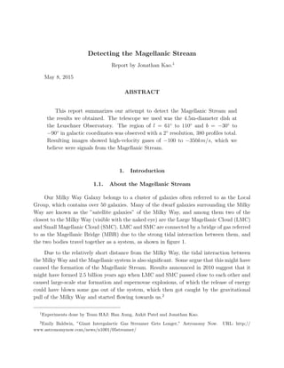
8. – 8 –
4. Discussion
The most important thing to ask now is whether what we detected was in fact the
Magellanic Stream. Our 1D velocity map is again shown in figure 9, and we compare with
previous studies, figure 8 shows a velocity map from a study by Fox, Andrew J. et. al.. Since
the region we covered was approximately the upper half of the map in figure 8, comparing
the velocities we can say that the results are fairly close. In both figures we see that the
highest velocities occur at around b = −40◦
to −50◦
with peak values of −350km/s or above,
and velocity approaches 0km/s as we get closer to the pole at b = −90◦
. With similar values
in velocity and similar distributions, we would argue that even though the measurements
may not be accurate, what we detected was indeed the Magellanic Stream.
Fig. 8.— Velocity Map of the Magellanic
Stream. Figure credit: Fox, Andrew J. et al.,
”Exploring the Origin and Fate of the Magel-
lanic Stream with Ultraviolet and Optical Ab-
sorption,” Astrophys.J. 718 (2010) 1046-1061.
Fig. 9.— 1D Image - Velocity: this figure
shows our 1D velocity map of the region ob-
served. It is the same as figure 5.

9. – 9 –
However, there were some problems with the data we obtained that could have made our
relative intensity map inaccurate. While the setup of the telescope at Leuschner Observatory
sampled data with x-polarization and y-polarization, for unknown reasons the y-polarization
in the data we took did not reveal any useful information regarding the HI line. Therefore
we had to use the x-polarization only for calculating the intensity, and we believe that the
results are off. This was also why we made our images using relative intensities rather than
absolute values.
Lastly we would like to discuss whether the two trends we see make sense or not. As
described in section 3, the two trends we see are ”lower velocities” and ”higher intensities”
as we get closer to the pole at b = −90◦
. If we base the discussion on the understanding
we got from the background information described in section 1.1, since the gases get caught
by the Milky Way’s gravitational pull, the older the age (age meaning how long since the
gas escaped from the Magellanic System) the higher the velocity (negative). Additionally,
we might also expect the regions closer to the Magellanic System having higher intensities.
Knowing that b = −30◦
is the furthest and b = −90◦
is the closest to the current position
of the Magellanic Clouds, it seems reasonable to see higher velocities towards the b = −30◦
end and higher intensities towards the b = −90◦
end.
5. Conclusion
There were a few things that could definitely have been improved, and a few difficulties
that could be solved under different circumstances. With the radio dish at Leuschner being
brand new (for a nice photo see figure 10), we could not be sure whether the telescope would
work as expected, and the intensity calibrations we did within this short period of time were
probably not accurate enough. Also, the signal from the Magellanic Stream was so weak
that we had to take a total of more than 60 hours of data to cover the whole region, which
meant that there were no chances to closely examine the data and retake data to replace
the bad ones. However, even though we could not say for sure that we accurately observed
the Magellanic Stream, we are proud to say that we did actually detect something from the
Stream. We could definitely make more accurate measurements if we had more time.

10. – 10 –
6. Appendix - Photos
Fig. 10.— Professor Carl Heiles with the new 4.5m-diameter dish at Leuschner Observatory.
We can see the old dish down on the ground next to the new dish. Photo by Jonathan Kao.
Fig. 11.— Team HAJ presents: a scenic shot of the famous water tank with no water at
Leuschner Observatory. Photo by Jonathan Kao.