1. Tooth Growth Dataset Analysis
John Slough II
9 Jan 2015
We were asked to analyze the Tooth Growth dataset in R. From the R help file: “the response is the length
of odontoblasts (teeth) in each of 10 guinea pigs at each of three dose levels of Vitamin C (0.5, 1, and 2 mg)
with each of two delivery methods (orange juice or ascorbic acid).” The variable “len” is the tooth length in
mm, “supp” is the supplement type delivery method (OJ = orange juice, VC = ascorbic acid), and “dose” is
the dose level of vitamin C (0.5, 1, 2 mg).
Exploratory Data Analysis
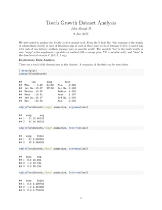
There are a total of 60 observations in this dataset. A summary of the data can be seen below.
library(plyr)
summary(ToothGrowth)
## len supp dose
## Min. : 4.20 OJ:30 Min. :0.500
## 1st Qu.:13.07 VC:30 1st Qu.:0.500
## Median :19.25 Median :1.000
## Mean :18.81 Mean :1.167
## 3rd Qu.:25.27 3rd Qu.:2.000
## Max. :33.90 Max. :2.000
ddply(ToothGrowth,"supp",summarize, avg=mean(len))
## supp avg
## 1 OJ 20.66333
## 2 VC 16.96333
ddply(ToothGrowth,"supp",summarize, StDev=sd(len))
## supp StDev
## 1 OJ 6.605561
## 2 VC 8.266029
ddply(ToothGrowth,"dose",summarize, avg=mean(len))
## dose avg
## 1 0.5 10.605
## 2 1.0 19.735
## 3 2.0 26.100
ddply(ToothGrowth,"dose",summarize, StDev=sd(len))
## dose StDev
## 1 0.5 4.499763
## 2 1.0 4.415436
## 3 2.0 3.774150
1

2. ddply(ToothGrowth,c("supp","dose"),summarize, avg=mean(len))
## supp dose avg
## 1 OJ 0.5 13.23
## 2 OJ 1.0 22.70
## 3 OJ 2.0 26.06
## 4 VC 0.5 7.98
## 5 VC 1.0 16.77
## 6 VC 2.0 26.14
ddply(ToothGrowth,c("supp","dose"),summarize, StDev=sd(len))
## supp dose StDev
## 1 OJ 0.5 4.459709
## 2 OJ 1.0 3.910953
## 3 OJ 2.0 2.655058
## 4 VC 0.5 2.746634
## 5 VC 1.0 2.515309
## 6 VC 2.0 4.797731
The first plot shows the tooth length by supplement type. From the boxplot, it appears that they are not
very dissimilar.
boxplot(ToothGrowth$len~ToothGrowth$supp,col=c("orange","green"),
main="Tooth Length by Supplement",ylab="Tooth Length (mm)",
xlab="Supplement (type)")
OJ VC
5101520253035
Tooth Length by Supplement
Supplement (type)
ToothLength(mm)
2

3. The next plot shows the tooth length by dose, 0.5, 1, and 2 mg. There does appear to be a difference between
these, especially between the 0.5 and 2 mg doses.
boxplot(ToothGrowth$len~ToothGrowth$dose,col=c("lightblue",
"blue","darkblue"),
main="Tooth Length by Dose",ylab="Tooth Length (mm)",xlab="Dose (mg)")
0.5 1 2
5101520253035
Tooth Length by Dose
Dose (mg)
ToothLength(mm)
The next plot shows the interaction between dose and supplement type. When dose is considered, it appears
that both supplement types increase the tooth length.
boxplot(len ~ interaction(supp,dose), data=ToothGrowth,
col=c("yellow","lightgreen","orange","green","salmon","darkgreen"),
main="Tooth Length by Dose and Supplement",ylab="Tooth Length (mm)",
xlab="Dose (mg) & Supplement (type) Interaction")
3

4. OJ.0.5 VC.0.5 OJ.1 VC.1 OJ.2 VC.2
5101520253035
Tooth Length by Dose and Supplement
Dose (mg) & Supplement (type) Interaction
ToothLength(mm)
Hypothesis Tests
There are many hypothesis tests that could be performed with this dataset. The plots above already give
an idea of which tests could prove to be siginificant. We can already surmise that for tooth length, there
is probably a highly significant difference between doses, but perhaps not a significant difference between
supplement types. Two sample t-tests were performed. The assumptions underlying this test are: The
populations from which the samples were drawn are normally distributed. The standard deviations of the
populations are equal. The samples were randomly drawn.
# T test for Supplement type
VC=subset(ToothGrowth, supp=="VC")
OJ=subset(ToothGrowth,supp=="OJ")
t.test(VC$len,OJ$len)
##
## Welch Two Sample t-test
##
## data: VC$len and OJ$len
## t = -1.9153, df = 55.309, p-value = 0.06063
## alternative hypothesis: true difference in means is not equal to 0
## 95 percent confidence interval:
## -7.5710156 0.1710156
## sample estimates:
## mean of x mean of y
## 16.96333 20.66333
# T test for doses
dose0.5=subset(ToothGrowth,dose==0.5)
dose2=subset(ToothGrowth,dose==2.0)
t.test(dose0.5$len,dose2$len)
4

5. ##
## Welch Two Sample t-test
##
## data: dose0.5$len and dose2$len
## t = -11.799, df = 36.883, p-value = 4.398e-14
## alternative hypothesis: true difference in means is not equal to 0
## 95 percent confidence interval:
## -18.15617 -12.83383
## sample estimates:
## mean of x mean of y
## 10.605 26.100
tdose=round(t.test(dose0.5$len,dose2$len)$p.value,14)
dose0.5=subset(ToothGrowth,dose==0.5)
dose1=subset(ToothGrowth,dose==1.0)
t.test(dose0.5$len,dose1$len)
##
## Welch Two Sample t-test
##
## data: dose0.5$len and dose1$len
## t = -6.4766, df = 37.986, p-value = 1.268e-07
## alternative hypothesis: true difference in means is not equal to 0
## 95 percent confidence interval:
## -11.983781 -6.276219
## sample estimates:
## mean of x mean of y
## 10.605 19.735
t.test(dose1$len,dose2$len)
##
## Welch Two Sample t-test
##
## data: dose1$len and dose2$len
## t = -4.9005, df = 37.101, p-value = 1.906e-05
## alternative hypothesis: true difference in means is not equal to 0
## 95 percent confidence interval:
## -8.996481 -3.733519
## sample estimates:
## mean of x mean of y
## 19.735 26.100
# T test for supplement and dose
VCdose.5=subset(ToothGrowth,dose==0.5 & supp=="VC")
OJdose.5=subset(ToothGrowth,dose==0.5 & supp=="OJ")
t.test(VCdose.5$len,OJdose.5$len)
##
## Welch Two Sample t-test
##
5

6. ## data: VCdose.5$len and OJdose.5$len
## t = -3.1697, df = 14.969, p-value = 0.006359
## alternative hypothesis: true difference in means is not equal to 0
## 95 percent confidence interval:
## -8.780943 -1.719057
## sample estimates:
## mean of x mean of y
## 7.98 13.23
VCdose1=subset(ToothGrowth,dose==1.0 & supp=="VC")
OJdose1=subset(ToothGrowth,dose==1.0 & supp=="OJ")
t.test(VCdose1$len,OJdose1$len)
##
## Welch Two Sample t-test
##
## data: VCdose1$len and OJdose1$len
## t = -4.0328, df = 15.358, p-value = 0.001038
## alternative hypothesis: true difference in means is not equal to 0
## 95 percent confidence interval:
## -9.057852 -2.802148
## sample estimates:
## mean of x mean of y
## 16.77 22.70
VCdose2=subset(ToothGrowth,dose==2.0 & supp=="VC")
OJdose2=subset(ToothGrowth,dose==2.0 & supp=="OJ")
t.test(VCdose2$len,OJdose2$len)
##
## Welch Two Sample t-test
##
## data: VCdose2$len and OJdose2$len
## t = 0.0461, df = 14.04, p-value = 0.9639
## alternative hypothesis: true difference in means is not equal to 0
## 95 percent confidence interval:
## -3.63807 3.79807
## sample estimates:
## mean of x mean of y
## 26.14 26.06
Almost all of the t-tests performed resulted in significant differences in the means of the tooth length at the
p=0.05 level.
The t-test for the supplement type resulted in a p-value of 0.0606, just barely higher than the 0.05 significant
level. Here we have very slight evidence that the tooth length means of the supplement types are not
dissimilar.
We have strong evidence that dose results in different mean lengths for teeth. Between the 0.5 and 2.0 mg
dose, a p-value of less than 0.000000001 is produced. This is highly significant.
When dose and supplement are considered, there are two significant difference at the 0.5 and 1.0 mg dose
levels, between supplement types. The p-values for these tests (dose of 0.5 mg, by supplement type and dose
of 1.0 mg, by supplement type) were 0.0063586 and 0.0010384 respectively.
6

7. Conclusion
Overall, we can conclude that as the dose of vitamin C increases, so does the tooth length. The supplement
type only appears to play a significant role at the 0.5 and 1.0 mg dose levels.
7