1. 1
AAE 251 Final Project: Team PM-9
Konrad Goc, Ben Klinker, Jeff Mok, Monica Salunkhe, Drew Sherman, Tyler Woodbury
Nomenclature
𝑇! = Thrust Required
𝑇! = Thrust Available
𝑃! = Power Required
𝑃! = Power Available
!
!
= Rate of Climb
𝑐! = Thrust Specific Fuel Consumption
𝑅 = Range
ℎ! = Geometric Altitude
𝜌 = Density
𝑞 = Dynamic Pressure
𝑣 = Velocity
𝐶! = Coefficient of Lift
𝐶! = Coefficient of Drag
𝐶!,! = Zero-Lift Drag Coefficient
𝑒 = Oswald Efficiency Factor
𝐴𝑅 = Aspect Ratio
𝑆 = Reference Area
𝑀 = Mach Number
𝑊 =Weight
𝑎 = Finite Lift Curve Slope
𝑎! = Infinite Lift Curve Slope
h = Height of Wing above Ground
b = Span
AFB = Air Force Base
∆𝑉 = Change in Velocity
∆𝑖 = Change in Inclination
𝜀 = Specific Energy
𝜇 = Gravitational Parameter of the Earth
r = Radius
a = Semi-major axis
LEO = Low Earth Orbit
g0 = Gravity at sea level
Isp = Specific impulse
finert = Inert mass fraction
SRB = Solid rocket booster
SEC = Single Engine Centaur
Ve = Exhaust velocity
ṁs = Mass flow rate of solid rocket booster
ṁl = Mass flow rate of liquid core stage
min,c = Inert mass of core stage
min,b = Inert mass of booster stage
mprop,c = Propellant mass of core stage
mprop,b = Propellant mass of booster stage
m0,2 = Initial mass of second stage
x = Burn time relationship between booster and core
P = Period
R = Rotational Period of the Planet
∇ = Orbital Angle Shift

2. 2
I. Introduction
The purpose of the design is to develop an emergency crew rescue vehicle (ECRV) composed of both rocket
and aircraft components capable of executing orbital rescue maneuvers and atmospheric flight to a safe location. The
priorities of the process are to ensure the safety of the astronauts in distress and minimize the cost of the overall sys-
tem. To confront this challenge, the design team considers fuel and inert mass values for both phases of the mission
through both quantitative analysis and comparison to existing technology.
The orbital and launch dynamics phase of design require an analysis of rocket sizing parameters based on the
requisite orbital maneuvers and launch conditions. Restrictions on the astrodynamic mission phase include: posi-
grade or retrograde launch, ability to attain low Earth orbit (LEO), and transfer capabilities into a 1000 km orbit.
There are also restrictions on the launch conditions which prevent launch within 500 km or ±30° of a significant
population center. The assembled rocket must be capable of carrying the aircraft payload into orbit and returning to
Earth.
The objective of the atmospheric flight portion of the design is to develop an ECRV that has the capability
of transporting 4 people as well as their associated equipment from an initial altitude and speed of 30,000 ft and 400
mph to a United States Air Force Base (AFB) initially located a minimum distance of 500 km from the re-entry lo-
cation. A detailed aerodynamic analysis aiming to optimize flight altitude, cruise speed, airfoil, and landing distance
will define the ECRV. Using a comparison the selected design to existing technology, an appropriate solution is
implemented, ensuring the viability of the selected alternative.
II. Launch Site Analysis
The five primary launch sites considered for launch based on existing launch locations are Cape Canaveral
Air Force Station, FL, Andersen Air Force Base, Guam, Vandenberg Air Force Base, CA, Wallops Island Flight
Facility, VA, Reagan Test Site, Kwajalein Atoll, and Kodiak Island.1
It is necessary to research these primary sites to find the best location to launch the ECRV. Considering the
project requirements, the best location is one which has no substantial populations that are less than or equal to 500
km from its Air Force Base residing within ±30° of the selected launch direction. Along with these requirements, the
launching site should be close to the equator and must be able to launch in a west or east orbit. The ideal rocket
launch is near the equator because traveling in the eastward direction gets a velocity boost due to Earth’s west-to-
east spin. The rate of spin is highest on the equator and lowest on the poles. Launching closer to the equator reduces
the 𝛥 𝑉 to achieve into LEO which requires less fuel.
Vandenberg Air Force Base, CA and Kodiak Island are preferred for polar launch operations from the con-
sidered launch locations.1
However, a polar launch is not preferred in comparison to an easterly launch because it
will minimize the 𝛥 𝑉 the rocket gains from the Earth’s rotation. Based on this, launch locations optimized for an
easterly launch are more highly considered, eliminating Vandenberg Air Force Base and Kodiak Island. If the rocket
is launched on the west coast, it would either have to fly across the United States or would have to fly east-to-west
requiring a larger 𝛥 𝑉 to overcome the Earth’s west-to-east rotation. This is another reason to not consider Vanden-
berg Air Force Base, CA as the launch site.
Wallops Island is NASA’s primary flight facility for management and implementation of suborbital re-
search programs. This location is not used because its location is 37.93° N and 75.46° W, which is farther from the
equator than Andersen AFB.2
As a result of the fact that it is significantly north of the equator, the benefit from the
Earth’s rotation decreases, and the maximum plane change requirement increases. Reagan Test Site is not an AFB
but a Major Range Test Facility Base.3
It tests missiles and space experiments. So, this location is not used.
Cape Canaveral satisfies most of the design requirements mentioned before. Cape Canaveral Air Force Sta-
tion is located adjacent to Kennedy Space Center in Florida. It has a latitude and longitude of 28.45° N and 80.52°
W.2
It has an elevation of 3 m.2
It is on the east coast so there are no substantial populations on the east side of Cape
Canaveral. It is also closer to the equator than any other locations in the US. In addition, rockets have been success-
fully launched from this location in the past. There have been 3,182 missile and rocket launches from Cape Canav-
eral from July 24, 1950 through December 19, 1999.4
There is also a reliable launch infrastructure available at Cape
Canaveral Air Force Station.5
However, Cape Canaveral is not the selected ECRV launch location after an analysis of Andersen AFB in
Guam.2
It has a latitude of 13.57° N and longitude of 144.92° E2
, and is closer to the equator than Cape Canaveral,
with an elevation of 627 m.2
It is an island with no substantial populations that are within 500 km from its AFB re-
siding within ±30° of any possible launch inclination.2
In contrast, retrograde launches from Cape Canaveral are
rendered impossible by the presence of large population centers to the west. Therefore, launching from Andersen at
any azimuth is possible, with the only concern being the small islands to the northeast. The Mariana Islands and

3. 3
Rota have very small populations, but if required, the rocket is designed to launch at an angle such that there is no
chance of harming these populations. Andersen AFB has been used for 12 launches from 1957 to 1958.6
Also, An-
dersen AFB was a deployment site for ATTREX (Airborne Tropical TRopopause EXperiment)7
whose objective
was to study moisture and chemical composition in the region of the upper atmosphere where pollutants and other
gases enter the stratosphere and potentially influence our climate.8
This ensures the feasibility of the launch location
as it has been successfully used in the past. Though, Andersen AFB is the selected location for the ECRV launch, it
is difficult to access due to its distance from the US mainland. For the scope of the analysis, the distance is not con-
sidered and it is assumed that the launch infrastructure is setup successfully beforehand. The fact that Andersen is a
currently functional AFB, with adequate operations and staffing, this assumption is justified.3
III. Orbital Maneuver Analysis
A. Plane Change Analysis
Through analysis, the highest change in velocity for an orbital maneuver happens during a plane change.
The 𝛥 𝑉 from Hohmann transfers is far less than the 𝛥 𝑉 of the inclination change. Thus it is important that the
ECRV has the optimal plane change maneuver. Due to a wide launch azimuth, and a low latitude, the plane change
is minimized. The worst plane change is from Guam’s latitude to equatorial orbit or the change to polar orbit con-
sidering the Mariana Is-
lands. However, many
launch sites do not offer
complete flexibility with
the azimuth inclination.
Guam offers the
best option for reducing the
plane change 𝛥 𝑉. The
𝛥 𝑉 for the plane change is
found for the worst possible
orbital maneuver that the
ECRV needs to accom-
plish. The Rota and the
Northern Mariana Islands
are located to the northeast
of Guam.2
Since the popu-
lations of the islands are
small, there is a high possi-
bility the rocket can launch over them. In the scenario where the launch path cannot cross these islands, the worst
plane change is 30°. Once in orbit, the optimal plane change is at apoapsis, where 𝛥 𝑉 is smallest. This is because the
velocity of the orbit is smallest at the apoapsis, so according to Eq. (1), the slower the velocity at the plane change
location, the smaller the required ΔV is.
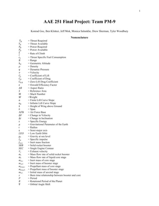
Fig. (1) demonstrates the relation between the maximum plane change and the 𝛥 𝑉 required by the ECRV to
make that plane change.
Using Guam as the launch site, the maximum 𝛥 𝑉 required for a plane change can be calculated using Eq. (1)
𝛥 𝑉!"#$% !!!"#$ = 2 ⋅ 𝑉!"#$#%&' ⋅ 𝑠𝑖𝑛
∆!
2
Eq. (1)
The 𝛥𝑖!"# is 30° at the maximum inclination, and assuming the plane change is performed at LEO, the 𝛥 𝑉 to make
this maneuver at 200 km altitude is 4.14 km/s.
B. Azimuth Launch Analysis
Figure 1. Required ΔV depending on plane change.

4. 4
In addition, the azimuth of the
launch affects the 𝛥 𝑉 needed to launch
the ECRV into LEO. Both retrograde
and posigrade orbits need are included
when accounting for the azimuth. Thus
the possible angles for the azimuth of
the ECRV launch range from -90° to
90°. The graph demonstrates the rela-
tionship between azimuth launch angle
and 𝛥 𝑉 required to get to LEO. 𝛥 𝑉 is
minimized at a 90° azimuth due to the
beneficial 𝛥 𝑉 from the rotation of the
Earth. Based on Fig. (2), it is beneficial
for the ECRV to launch into a posi-
grade orbit, greatly reducing the 𝛥 𝑉
required to get into LEO. The ECRV ’s
design accounts for the possibility of a
retrograde azimuth launch because that
is the azimuth launch where 𝛥 𝑉 is the
greatest. Note that Fig. (2) does not account for the 𝛥 𝑉 from the Hohmann transfer maneuver or from the deorbit
Hohmann transfer maneuver.
C. Hohmann Transfer Analysis
The orbital maneuvers for the Hohmann transfer require a much smaller 𝛥 𝑉 for the ECRV. This is the 𝛥 𝑉
for the rocket to reach its maximum altitude above the Earth. The 𝛥 𝑉 for the Hohmann transfer encompasses the
entire 𝛥 𝑉 to enter the transfer orbit and circularize into the larger orbit. Transferring into a 1,000 km altitude orbit
requires 0.43 km/s. By finding the
maximum change in velocity, the
ECRV can reach any possible orbit to
rescue a vehicle. Thus, the design of
the ECRV can reach the maximum
altitude of 1,000 km. The following
equations describe the process for
finding the Hohmann transfer:
𝜀 =
!
!!
𝐸𝑞. (2) 𝜀 =
!!
!
!
−
!
!!
𝐸𝑞. (3)
∆𝑉! = 𝑉! − 𝑉!,! 𝐸𝑞. (4) ∆𝑉! =
𝑉!,! − 𝑉! 𝐸𝑞. (5)
𝑉!,! =
!
!!,!
𝐸𝑞. (6) ∆𝑉!"!#$ = ∆𝑉! + ∆𝑉! 𝐸𝑞. (7)
D. Deorbit Maneuver Analysis
Figure 3. Relation of Altitude and 𝛥 𝑽 for Hohmann transfer.
and 𝛥 𝑽.
Figure 2. Relation between Azimuth Launch Angle.
and 𝛥 𝑽.

5. 5
The ECRV must return to the
Earth by placing the periapsis of its orbit
inside the radius of the Earth. This maneu-
ver corresponds to a 𝛥 𝑉 value from a se-
cond Hohmann transfer. The ECRV does
not need to make an additional plane
change during its deorbiting maneuver.
Even in a 90° polar orbit, the ground track
will still land within the 2,500 km range of
the aircraft within 24 hours. The value of
𝛥 𝑉 for the deorbiting maneuver is 0.55
km/s. This deorbiting maneuver is calcu-
lated using the condition that the ECRV is
at its maximum altitude (1,000 km). Simu-
lating deorbit from the farthest distance ensures the feasibility of any distance between the Earth and the maximum
orbit. The purpose of deorbiting is to land the ECRV safely in Guam. Fig. (4) demonstrates this relationship between
deorbit and 𝛥 𝑉.
E. Total ∆𝑽 Analysis
Finally, there are multiple components of 𝛥 𝑉 in the final calculation to find the final value for 𝛥V!"!#$.
The equations Eq. (8) and Eq. (9) below find 𝛥 𝑉 𝑡𝑜𝑡𝑎𝑙:
𝛥 𝑉 𝑡𝑜𝑡𝑎𝑙 = ∆𝑉 𝐿𝐸𝑂 + ∆𝑉 𝑝𝑙𝑎𝑛𝑒 + ∆𝑉 𝐻𝑜ℎ𝑚𝑎𝑛𝑛 + ∆𝑉 𝑑𝑒𝑜𝑟𝑏𝑖𝑡 𝐸𝑞. (8)
𝛥 𝑉 𝐿𝐸𝑂 = ∆𝑉 𝑑𝑟𝑎𝑔 + ∆𝑉 𝑔𝑟𝑎𝑣𝑖𝑡𝑦 + ∆𝑉 𝑠𝑡𝑒𝑒𝑟𝑖𝑛𝑔 + ∆𝑉 𝑎𝑧𝑖𝑚𝑢𝑡ℎ + ∆𝑉𝑖𝑑𝑒𝑎𝑙,𝐿𝐸𝑂 𝐸𝑞. (9)
The maximum 𝛥 𝑉 for all
launch conditions, possible
orbital maneuvers, and deorbit
maneuvers is 15.20 km/s. This
𝛥 𝑉 is the absolute worse case
scenario for the ECRV. Thus,
if the ECRV can accomplish
the rescue under these condi-
tions, it can make the same
rescue maneuvers for any oth-
er orbit within a 1,000 km
altitude. Fig. (5) shows the
maximum 𝛥 𝑉 the ECRV per-
forms.
In summary, the 𝛥 𝑉
for the ECRV changes with
many different variables. Ta-
ble (1) shows a breakdown of 𝛥 𝑉 values for different portions of the rescue. As shown, the main factors are plane
change and azimuth angle.
∆𝑉!"!#$ 𝛥 𝑉 𝑝𝑙𝑎𝑛𝑒 𝑐ℎ𝑎𝑛𝑔𝑒 ∆𝑉!"# 𝛥𝑉!"!!"## 𝛥𝑉!"#$%&'
Posigrade 14.35 km/s 4.14 km/s 9.22 km/s 0.4338 km/s 0.5545 km/s
Retrograde 15.20 km/s 4.14 km/s 10.08 km/s 0.4338 km/s 0.5545 km/s
Table 1. Values of 𝛥 𝑽 for Different Orbital Maneuvers.
Figure 5. Relation of 𝛥 𝑽 and Plane Change Maneuver.
and 𝛥 𝑽.
Figure 4. Relation of 𝛥 𝑽 and Altitude: Deorbit Maneuver
and 𝛥 𝑽.

6. 6
IV. Rocket Analysis
A. Third Stage / Capsule Design
The ECRV must reach LEO and maneuver to the location of the crew. The rescue can be accomplished in
many ways, such as multi-staging or rocket-like planes. Minimizing weight is an important factor in designing a
rocket. In addition, accommodating the absolute worst-case scenario is imperative, especially when trying to save
lives; therefore, all calculations and sizing are based off the worst-case scenario. This section discusses sizing, rock-
et models, design of the rocket, and transport to the crew.
The estimated ΔV is 15.20 km/s based upon a plane change of 30°, a 1,000 km rescue orbit and retrograde
launch. The rocket and rescue system must accommodate this maximum value. If the rocket design can handle the
worst possible ΔV, then anything less than 15.20 km/s is attainable. Since this is a large value, it is difficult to
choose how to design the system. Optimization becomes hard due to the possibility of a three-stage system. One
alternative is to have the third stage accomplish all orbital maneuvers, optimize its performance, and then optimize a
two-stage rocket using the third stage as a payload.
Designing the rocket requires a backward approach: the payload of the last stage must be sized before addi-
tional design begins. Analysis for the ECRV begins with the Virgin Galactic SpaceShipTwo. SpaceShipTwo is a
rocket-plane that can withstand partial re-entry and land like a conventional plane. These qualities make the craft a
good initial choice. The issues with SpaceShipTwo are twofold: it does not have enough fuel capacity to execute
many orbital maneuvers, and it is too large for most standard payload fairings. Finding the fuel needed for the ma-
neuvers is necessary for proving the feasibility of SpaceShipTwo. Calculating the ΔV required for the worst orbital
maneuver is shown by Eq. (10).
Δ𝑉!"#$%&$' = Δ𝑉!"#$!"%&!'" + Δ𝑉!"#!$%&#"'&(")* + Δ𝑉!"#$%&' 𝐸𝑞. (10)
A plane change of 30° (due to safety requirements of the launch location) and a Hohmann transfer of 1,000 km is the
most intensive maneuver. Adding the required circularization and deorbiting ΔV, the total change in velocity is Eq.
(11).
Δ𝑉!"#$%&$! = 0.2200 + 4.1336 + 0.2138 + 0.5545 𝑘𝑚/𝑠 Eq. (11)
Considering the required ΔV for all the orbital maneuvers is 5.10 km/s, using an estimated specific impulse of 448 s
and an finert of 0.15, using the rocket equation, Eq. (12) and Eq. (13):
𝑀!"#! =
𝑀!"#(𝑒!!/(!!∗!!")
− 1)
(1 − 𝑓!"#$% 𝑒!!/(!!∗!!")
)
𝐸𝑞. (12)
the required fuel mass is approximately 12,000 kg, which exceeds the full 10,000 kg capacity of SpaceShipTwo.9
This mass requires the use of something more powerful than SpaceShipTwo, bringing into question the original idea
of using a system similar to a rocket-plane. Due to the high ΔV requirement, a craft similar to a third stage of a rock-
et must be considered.
B. Rocket Sizing Analysis
Capsules are generally the payload of two or three stage rockets. It is therefore viable to consider using a
capsule that envelops the rescue craft to perform the required orbital maneuvers. Since the capsule can be designed
independently of the craft, analyzing the best propulsion systems is necessary. According to the rocket equation, Eq.
(13), specific impulse is an extremely important parameter. Specific impulse describes how long one kilogram of
fuel can produce one Newton of thrust. Thus a high specific impulse and high thrust values are ideal because they
reduce the amount of fuel needed. The J-2X engine is a great example of an engine to use. With an Isp of 448 s and a
thrust level of 1,310,000 N, it is unrivaled in terms of performance. Other engines such as the RL-10 are valid op-
tions. The RL-10 provides 465 s Isp but only 110,000 N of thrust.10
Thus the J-2X is the choice of engine for the cap-
sule. Since space-planes cannot carry enough fuel to perform the ΔV, the capsule must carry the ECRV, adequate
fuel for the orbital maneuvers, and the heat shield for re-entry. Using the 3,500 kg mass of the aircraft (see aircraft
analysis) and Eq. (13) and Eq. (14):

7. 7
𝑀! =
𝑀!"# 𝑒
!!
!!∗!!"(1 − 𝑓!"#$%)
1 − 𝑓!"#$% 𝑒!!/(!!∗!!")
𝐸𝑞. (13)
𝑀! =
3,500𝑒
!"##
!.!"∗!!"(1 − .15)
1 −. 15𝑒!"##/(!.!"∗!"")
𝐸𝑞. (14)
The total mass of the capsule is 17,640 kg. This mass includes approximately 12,000 kg of fuel for orbital maneu-
vers, the mass of the J-2X, the mass of the ECRV, and the inert mass of the capsule. The capsule enters LEO for the
checkout orbit where it performs systems checks. These checks include ECRV flight systems inspection, capsule
heat shield inspection, structural inspection, and electronic systems tests. The capsule then executes any Hohmann
transfer up to 1,000 km, performs a plane change, circularizes the orbit, and rendezvous with the crew. Once the
crew enters the ECRV, the capsule conducts a deorbiting burn, re-enters the atmosphere, and releases the ECRV at
30,000 ft.
With the total mass of the capsule, designing the rocket is now possible. Due to the need to accomplish any
ΔV up to 10.13 km/s, a high-capacity rocket is necessary. A large two-stage rocket is adequate, as three-stage sys-
tems such as the Space Launch System and Saturn V are too large. Researching common two-stage rockets results in
a few rockets to consider: the Atlas V 541, the Delta IV Heavy, and the Falcon Heavy. These rockets can handle
payloads greater than the mass of the capsule, thus making them viable. Analyzing the Atlas V 541 shows that the
required configuration for a high payload is four Aerojet SRBs and a Lockheed Martin CCB (common core booster)
with an SEC (single engine Centaur) upper stage.11
The Centaur upper stage uses an RL-10 engine and achieves an
Isp of 460 seconds.11
Finding the specific impulse of the parallel first stage requires taking an average of the Isp, by
weighing the mass flow rates in Eq. (15):
𝐼!",! =
(𝐼!",! +
ṁ!
ṁ!
𝐼!",!)
(1 +
ṁ!
ṁ!
)
𝐸𝑞. (15)
the weighted average Isp of the parallel first stage is 249 seconds. To reduce the initial mass, a first stage with a
higher specific impulse is beneficial. The Delta IV Heavy uses high specific impulse CCB engines, similar to the
Atlas V. The benefit comes from a much higher specific impulse due to using liquids instead of solids, theoretically
decreasing the mass required. Using three CCBs and a single SEC, the total liftoff mass is decreased.12
Another
rocket to consider is the Falcon 9 Heavy. It utilizes in-house SpaceX Merlin engines, which have a low Isp, and ac-
cording to the rocket equation, are very inefficient at decreasing liftoff mass.13
The finert values from the Falcon 9
Heavy are very low, making a mixture of engines and Falcon 9 liquid tanks the ideal choice. Using more efficient
engines with high-efficiency liquid tanks reduces the maximum takeoff mass on the Falcon 9 Heavy and results in
an extremely efficient rocket. Since the second stages ignite while still partially in atmosphere, a correction factor of
0.90 times the Isp of the second stage in a vacuum is a realistic Isp estimation for the duration of the flight.
(first stage, second stage)
Atlas V 541 (4
SRBs, CCB,
SEC)11
Delta IV Heavy (3
CCB, SEC)12
Falcon 9 Heavy (3
block II Falcon 9,
block II Falcon 9)13
Falcon 9 Heavy
(RS-68A, RL-10)
Isp (s)
249, 460*.90
360, 460*.90
304, 336*.90
365,460*.90
finert
0.073, 0.089
0.110, 0.1150
0.0736, 0.0634
0.0736, 0.0634
Total liftoff mass (with
17640 kg payload) kg to
achieve 10,086 m/s ΔV
787,221
594,228
1,153,960
376,212
Table 2. Comparison of Heavy Two-Stage Rockets for Retrograde Launch

8. 8
Table (2) shows the modified Falcon 9 Heavy with RS-68A engines on the first stage boosters and an RL-
10 on the second stage is the most efficient rocket. Due to the rocket equation, the finert and Isp values play a huge
role, so optimizing them results in an optimized rocket, as shown by the modified Falcon 9 Heavy. While that par-
ticular rocket does not exist, all components are used on current generation rockets, and can be used for launching a
rescue vehicle.
A modified Falcon 9 Heavy is the cho-
sen rocket type for launching the capsule and the
ECRV into orbit. Using the rocket equation, the
total mass for a retrograde launch is 376,212 kg,
with 243,746 kg of fuel and 19,365 kg of inert
mass. As shown by Fig. (6), the ΔV for the first
stage is 3731 m/s (37%) and is supplemented by
6348 m/s (63%) from the second stage.
This split is due to the significantly
higher Isp of the second stage, which results in the
rocket equation requiring it to do more work.
Launching posigrade results in a huge decrease in
mass, down to 279,083 kg, if all other variables
stay constant, because the launch azimuth is 90°.
Launching posigrade is certainly preferable, but
if required, the rocket can launch retrograde at
the cost of more mass.
C. Parallel Staging Analysis
It is worth noting that the Falcon 9
Heavy is parallel-staged, which requires analysis of the staging and how it might affect the initial mass. To analyze
parallel staging, the first stage is broken into two parts. This is due to the boosters separating before the core. As a
result, the finert and weight changes differently than in serial staging. When the boosters separate, there is still fuel
left in the core, this fuel is accounted for through a burn rate relationship (x). The equations below split the first
stage into a stage 0 and stage 1, where stage 0 Eq. (16) is with the boosters and stage 1 Eq. (17) is after they have
separated:
Δ𝑉! = −𝑉! ln
𝑚!",! + 𝑚!",! + 𝑥𝑚!"#!,! + 𝑚!,!
𝑚!",! + 𝑚!"#!,! + 𝑚!",! + 𝑚!"#!,! + 𝑚!,!
𝐸𝑞. (16)
Δ𝑉! = −𝑉! ln
!!",!!!!,!
!!!"#!,!!!!",!!!!,!
𝐸𝑞. (17) 14
Analyzing the parallel stages results in a
mass higher than if it were simply serial
staged. Fig. (7) shows that parallel staging
the first stage is most efficient when the
core stage contributes 100% of the ΔV.
This leads to the conclusion that parallel
staging is not beneficial for reducing mass
compared to a serial-staged two-stage
rocket. Parallel staging does significantly
affect sizing when compared to three-stage
rocket, because it can achieve the same
effect as three stages, but with a smaller
rocket. While the Falcon 9 Heavy is paral-
lel staged, it can be treated like a large first
stage and normal second stage for rocket
equation analysis. Parallel staging has ben-
efits when considering time to orbit, struc-
Figure 7. ΔV Split for Parallel Staging.
First Stage
Figure 6. Total Mass vs ΔV Split of Stage 2.

9. 9
ture complexity, and fuel transfer, but does not reduce the initial mass. Since the rocket analysis is based on reduc-
ing mass at launch, parallel staging is not a viable option.
D. Payload Fairing and Design
The modified Falcon 9 Heavy appears to be a great choice for launching the ECRV and capsule into orbit.
To ensure the rocket can meet the capsule’s needs, the payload fairing needs to be large enough to fit the capsule
containing the ECRV. The Falcon 9 Heavy utilizes a 5.2 m diameter payload fairing with a usable width of 4.6 m.
Its length is 13.1 m, with 11.4 m usable for the capsule.15
Since the wings of the ECRV can fold, the widest point is
the horizontal stabilizer at 3.8 m. The tallest point is 2.7 m, and its length is 9.0 m. This leaves enough room for the
capsule and the J-2X, with room for propellant storage tanks next to the ECRV.
E. Rocket Cost Analysis
An estimated rocket cost is calculated from the inert and propellant masses. Since launch mass depends
heavily on the launch azimuth (retrograde versus posigrade), two different cost analyses of the rocket are necessary:
Table 3. Cost analysis of worst-case retrograde and posigrade rocket launches
V. Re-entry Analysis
Posigrade Costs ($)
Retrograde Costs ($)
Inert Mass
13,156kg *
$1000/kg
13,156,000
19,365kg *
$1000/kg
19,365,000
1st stage propellant
165,592kg *
$20/kg
3,311,840
243,746kg *
$20/kg
4,874,920
2nd stage propellant
77,452kg *
$20/kg
1,549,040
89,409kg * $20/kg
1,788,180
3rd stage propellant
12,000kg *
$20/kg
240,000
12,000kg * $20/kg
240,000
Total Cost ($)
18,256,880
26,268,100
Figure 3: Payload fairing containing the capsule, J-2X, ECRV, and fuel tanks

10. 10
Calculations of orbital periods and ∇s for each orbit demonstrate the limits of the possible orbits in the mission. Note
inclination has no impact on orbital period or ∇.
𝑃 =
2𝜋𝑎
!
!
𝜇
𝐸𝑞. (18)
𝛻 =
𝑃
𝑅
360° 𝐸𝑞. (19)
Altitude (km) Period (min.) ∇(degrees)
200 88.49 22.12
1,000 105.12 26.27
Table 4. Period and ∇ at 200 kilometer and 1000 kilometer altitude circular orbits.
For the re-entry maneuver, Guam’s location of 13.57° N latitude and 144.92° E longitude is convenient.2
The amplitude of inclination corresponds to the maximum latitude that the orbit crosses, thus the deorbit analysis
consists of two parts. The farthest longitudinal distance from Andersen Air Force Base deployment could occur is
half of the maximum ∇, for any orbit more than 13.57° inclination. With a maximum ∇ of 26.27°, the longest lon-
gitudinal distance that would have to be traveled is 13.14° or 1,462.15 km. Re-entry and deployment of the ECRV
can occur from any circular orbit from 200 km to 1,000 km. The maximum latitudinal distance required to travel by
the aircraft from deployment to landing at Anderson Air Force Base in Guam is 1,511.25 km, for any orbit less than
13.57° inclination. This instance occurs at equatorial circular orbit, where the aircraft would deploy from the equator
at 144.92° E and travel directly north to Andersen AFB. The mission is an emergency, therefore time is an important
factor. Therefore, deployment can occur at the first ground track pass of Guam and the aircraft will be capable of
safely landing at the launch location. The maximum longitudinal and latitudinal distances occur in separate cases.
This maximum travel distance falls below the upper range limit of 2,500 km.
V. Aircraft Analysis
A. Aircraft Engine Analysis
The primary constraints applying to the ECRV include cost, weight, and size of the aircraft. These stipula-
tions originate from the ECRV requirements of safe travel into low earth orbit as a payload on a rocket. Using the
rocket equation, mass increases exponentially with added weight, thus the design process begins by minimizing the
inert mass of the ECRV. For the purposes of this analysis, there are no detailed aerodynamic calculations describing
the inert mass or structure of the fuselage. Instead, a comparison to existing technology serves to optimize the pa-
rameters of the aircraft aimed at minimizing the weight. In contrast to this, an aspect of the aircraft structure that
falls within the scope of analysis is the engine type and its characteristics which include thrust specific fuel con-
sumption, weight, and thrust produced. The initial approach to optimizing the engine parameters involves finding
the minimum thrust required at a given flight altitude (re-entry altitude or 30,000 ft). For a range of reasonable
cruise velocities of the aircraft, the thrust required to maintain steady and level flight is computed as:
𝑇!,!"# =
𝜌!"#
𝜌!"#
𝑤!
𝐶! 𝐶!
𝐸𝑞. (20)
Eq. (20) uses the initial value of the weight to calculate the thrust required to fly at a given altitude. The weight re-
mains constant for the duration of the steady and level flight. Since the only change in mass of the ECRV occurs as a
result of burning fuel, the constant mass assumption is reasonable. If the initial fuel mass of the aircraft is small. Eq.
(20) requires the lift to drag ratio from the following equations:
𝑞! =
1
2
𝜌! 𝑣!
𝐸𝑞. (21)
𝐶! =
𝑤
𝑞! 𝑆
𝐸𝑞. (22)
𝐶! = 𝐶!,! +
𝐶!
!
𝜋𝑒𝐴𝑅
𝐸𝑞. (23)
Eq. (21) refers to the dynamic pressure given an aircraft cruise velocity and atmospheric density. Studies of the vari-
ation of these parameters with respect to aspect ratio estimate the zero lift drag coefficient 𝐶!,! and Oswald effi-
ciency factor 𝑒 of the aircraft as 0.02 and 0.85 respectively.16,17
Using this information, Eq. (22) and (23) calculate
the lift to drag ratio taking into account the effects of both the finite wing (induced drag as a result of the pressure

11. 11
difference between the upper and lower surface of the wing tip) and aircraft structure (manufacturing imperfections
and any structure protruding from the main body of the ECRV). Both decrease the overall aerodynamic efficiency of
the aircraft, but yield a more representative analysis of the aerodynamic profile of the ECRV. Due to the possibility
of velocities above 100 m/s, the Prandtl-Glauert correction factor is used to account for the change in air density as it
flows over the top surface of the cambered wing. In this scenario, the incompressible flow assumption is not true,
unlike with speeds below 100 m/s. This value serves as a benchmark for analysis of airflow in the transonic regime
rather than a value that describes a rigidly defined transition. Eq. (24) demonstrates an application of the correction
factor to an arbitrary aerodynamic coefficient, denoted by 𝐶!, as follows:
𝐶!,!"##$!%$& =
1
1 − 𝑀!
∗ 𝐶! 𝐸𝑞. (24)
Eq. (24) computes a range of adjusted lift to
drag ratios at sea level for use in Eq. (20). Eq.
(20) scales the thrust required values for a
cruise altitude with a corresponding density
value computed using the standard atmos-
phere function. This scaling is visible in Fig.
(8). This plot demonstrates the increasing
thrust required to fly at a constant velocity as
flight altitude increases. To minimize the
weight of the aircraft, the weight of the en-
gine must be minimized as well. Since engine
weight increases with available thrust, the
weight is minimized at the lowest thrust val-
ue. From the Fig. (8), the available thrust of
the engine is selected by finding the mini-
mum thrust required at the flight and the
cruise velocity since each thrust value corre-
sponds to a velocity. At this thrust value,
the aircraft barely sustains flight at the
specified altitude. The feasibility of this
thrust value is tested by comparing this value to the thrust required so that the service ceiling of the aircraft is equal
to or greater than the desired cruise altitude. For the case of the ECRV, this desired value is assumed to be the re-
entry altitude due to the fact that range is maximized at higher altitudes due to the decreased density of air.18
B. Climb Characteristics
Next, the climb characteristics of the aircraft are computed by making several assumptions. For example,
assume that the available thrust of a turbojet engine is constant and that the limit of altitude for the aircraft is the
service ceiling. This is where the maximum rate of climb is 100 ft/min and provides a more useful analysis than the
absolute ceiling, the altitude at which maximum rate of climb is 0.0 ft/min. This altitude can take a long time to
reach and will not provide a useful metric in determining the necessary engine characteristics. The maximum rate of
climb at a particular altitude is the maximum difference between power available and power required. The service
ceiling is the corresponding altitude at which the rate of climb value is 100 ft/min. Based upon this information, the
climb characteristics (rate of climb, time to climb, service ceiling) are computed using the following equations:
𝑅
𝐶
=
𝑃! − 𝑃!
𝑊
= 𝑉𝑠𝑖𝑛𝜃 𝐸𝑞. (25)
𝑡!"#$% =
𝑑ℎ
𝑅 𝐶
𝐸𝑞. (26)
!!
!!
𝑃! =
2𝑊! 𝐶!
!
𝜌𝑆𝐶!
! 𝐸𝑞. (27)
Figure 8. Variation of required thrust with freestream velocity.

12. 12
Table 5. Chart of researched lightweight aircraft.
Power required is adjusted for altitude using the standard atmosphere function using Eq. (27). Power available is
thrust available multiplied by freestream velocity and is proportional to air density at a given altitude. Due to the
initial assumption of constant thrust, the power
available is a line of constant slope and is plotted
concurrently with power required at various alti-
tudes. This relationship is visible in Fig. (9). The
maximum excess power is computed at each new
altitude to find the maximum rate of climb. Eventu-
ally, this rate of climb decreases below 100 ft/min.
The objective of this analysis is to size an engine
with minimum available thrust that is capable of
flying at an altitude of 30,000 ft. This will help to
minimize the weight of the aircraft. To ensure the
feasibility of the aircraft engine parameters, several
existing aircraft are shown in Table (5) and from
this list, the aircraft with parameters most closely
resembling that of the required engine will be se-
lected. The parameters of investigated aircraft in-
clude an ability to seat the four rescued astronauts,
a service ceiling above 30,000 ft and a size such
that the aircraft is able to fit into the rocket payload
fairing.
Table (5) only considers light-weight aircraft.
This is a key parameter to optimize cost, rocket
fuel weight, and ECRV range. The primary
motivation for Table (5) lies in analyzing feasi-
ble engine alternatives. From the viable alterna-
tives, the PiperJet Altaire with the Williams
FJ44 turbofan engine is used to justify the rea-
sonability of the engine thrust value. The air-
craft is also selected because it utilizes a single
turbofan engine which is key because a turbo-
fan produces more thrust than a turboprop, but
at a lower efficiency, allowing for flight to a
higher service ceiling. The use of only one en-
gine also minimizes the inert mass of the air-
craft by a significant amount. In reality, the
PiperJet is a discontinued model due to safety
concerns from the FAA in regards to the air-
craft’s single engine design with a relatively
high service ceiling.19
Therefore, there are no
backup alternatives if the engine malfunctions
Plane Name Engine Service
Ceiling [ft]
Thrust [N] Wingspan
[m]
Mass
(max) [kg]
PiperJet Al-
taire19
Williams FJ44 35,000 6,600 13 3,288
Cessna 17220
Lycoming-O360 13,500 2,000 11 1,113
Beechcraft
Premier I21
Williams FJ44-2A 41,000 10,230 13.5 5,670
Cirrus Vision
SF5022
Williams FJ33 28,000 8,500 12 2,722
Figure 9. Computation of maximum excess power.
Figure 10. Maximum Rate of Climb of ECRV as function
of altitude.

13. 13
during flight. For the purposes of the project, this is an acceptable risk as the aircraft will be used sparingly over
time, minimizing the wear on the engine, and will also be serviced and maintained on a regular basis (these costs are
included in the Jet A fuel cost).
The initial mass of the aircraft
includes: mass of the rescued astronauts
and associated equipment, inert mass of
the aircraft, and fuel mass. To provide a
reasonable approximation for this value,
use the maximum mass of the PiperJet.
Because the astronauts and the equip-
ment will weigh significantly more than
the typical passenger load of the PiperJet,
the dimensions of the aircraft must be
adjusted to fit the dimensions of the pay-
load fairing in the rocket. To accomplish
this, the length of the aircraft must be
shortened to 10 m and the wingspan
shortened to 10 m. A decrease in the
dimensions of the aircraft keeps the max-
imum mass constant; however, additional
structure required for launch and re-entry
makes this maximum mass 3,500 kg.
A quantitative analysis of the
time to climb and service ceiling is pos-
sible with the dimensions, mass, and
thrust. These values differ from existing
PiperJet specifications due to the aforementioned modifications that ensure the success of the rocket based phase of
the mission. Fig. (10) and Fig. (11) come from Eq. (25) and Eq. (26). Based on the altered PiperJet specifications,
the service ceiling is visible in Fig. (10) as the altitude where the maximum rate of climb reaches 100 ft/min. The
time to climb is the area under the curve in Fig. (11) taken from sea-level to the service ceiling. The maximum rate
of climb, service ceiling, and time to climb values of the ECRV are 51.34 ft/sec at sea level, 35,843.55 ft (consistent
with the data in Table (5)), and 43.31 min respectively. Although the time to climb and maximum rate of climb val-
ues do not apply to the ECRV rescue mission, they are critical for creating a comprehensive aerodynamic profile of
the proposed vehicle. The service ceiling, on the other hand, is a crucial value for the purposes of design as the air-
craft must achieve powered flight at the specified cruise altitude, which is the same as the re-entry altitude. A service
ceiling above the cruise altitude is critical in order to ensure the safety of the mission; however, the difference be-
tween these values should be small to ensure a low engine weight. The service ceiling of this mission acts to both
ensure the safety of the aircraft at the cruise altitude as well as to optimize the overall weight of the aircraft.
C. Range Analysis
Another factor that must be taken into account when considering the mass of the aircraft is the fuel required
to travel a specified range. Upon deployment, the aircraft must have enough fuel to land safely at an existing United
States AFB. For an aircraft of the previously described parameters, the maximum attainable range is about 2,500
km.19
This means that the aircraft must de-orbit within 2,500 km but more than 500 km of a substantial population
center (to guarantee safety in the case of a failed re-entry) from the AFB. For the purpose of fuel mass calculation,
the range equation is used because the only change in mass of the aircraft is accounted for by burning fuel.
𝑅 = 2
2
𝜌! 𝑆
1
𝑐!
𝐶!
𝐶!
𝑊! − 𝑊! 𝐸𝑞. (28)
Figure 11. Inverse of Maximum Rate of Climb of ECRV as func-
tion of altitude.

14. 14
Eq. (28) can be rearranged to find the final weight of the aircraft given a required range, which for the ECRV must
be at least 500 km and can be as much as the maximum range of the actual aircraft which is about 2,500 km. For this
reason, the de-orbit must be constructed to place
the aircraft within this maximum range value
from the AFB. The analysis shows that with an
increase in required range, the final weight of the
aircraft decreases, meaning that more is burned to
fly the increased distance. This relationship is
justified by Fig. (12). To ensure the safety of the
passengers, fuel must be included to perform
flight for the worst-case range scenario, which
based upon existing technology is roughly 2,500
km. Using flight at 30,000 ft altitude for 2,500
km, the required fuel mass is 443.50 kg which is
minimized due to the small size of the aircraft.
Because the fuel is less than 5% of the total mass,
the assumption that mass is constant for the
duration of the steady and level flight is
appropriate. During the design of the ECRV,
another consideration that aims to minimize fuel
mass decreasing the required range of flight by
the maximum gliding range. In this scenario,
only fuel for the powered phase of the flight is
included. The aircraft glides down to the AFB from the cruise altitude, thus decreasing the range of powered flight.
The gliding range is computed using the following equation:
𝑅!"#$% = ℎ! ∗
𝐶!
𝐶!
𝐸𝑞. (29)
The lift to drag coefficient for the gliding flight is recalculated using Eq. (23) and Eq. (24) using the final weight of
the aircraft at the end of the powered flight. Dynamic pressure corresponding to the cruise velocity is used. The lift
to drag ratio at the end of the powered flight serves as an approximation for the lift to drag ratio of the gliding flight.
Using Eq. (29), the gliding lift to drag ratio is 13.19 and the maximum gliding range is 120.58 km. By using Eq.
(28), with the new required range decreased by the gliding range, the new final mass yields a fuel savings of 20.70
kg. Due to the minimal fuel savings, gliding is used as a means to reach sea-level altitude and land at the AFB
instead of saving fuel. The risk of including too little fuel by decreasing the fuel mass outweighs the benefit of
saving roughly 20 kg of fuel. By including fuel for the entire range, there is a surplus of fuel remaining upon landing
rather than a shortage, allowing for extra flight maneuvers that are not considered in the range equation.
D. Aerodynamic Analysis
Now that most of the aircraft parameters are specified, it is necessesary to begin the aerodynamic analysis
of the ECRV. The first step in this process is to select the optimal airfoil that the aircraft will use. The approach is to
maximize the section lift to drag ratio of the infinite wing based on the available NACA airfoils present in Appendix
D.23
By maximizing the lift to drag ratio, a key parameter in any aerodynamic analysis, the aircraft will produce
sufficient lift to support its weight and maintain a high efficiency. This parameter is especially key in the ECRV
design because the craft will have a relatively small aspect ratio as a result of the dimensioning limitations of the
rocket payload fairing. A high lift to drag ratio is key to keeping landing distance relatively low. The selection of the
airfoil is based upon a computation of lift to drag ratio at a zero degree angle of attack for each of the available
NACA airfoils in Appendix D.23
For the purpose of this project, the lift curve slope with the Reynolds Number
represented by circles is used. The maximum ratio is found in the NACA 4415 airfoil. Since an airfoil is the
equivalent of an infinite wing, it is necessary to adjust the lift curve slope of the 4415 airfoil to establish a realistic
value to use in subsequent analysis for the finite wing of the ECRV. After computing the slope of the infinite lift
curve, the following equation is used to adjust the value for a finite wing:
Figure 12. Variation of final aircraft mass with range.

15. 15
𝑎 =
𝑎!
1 +
𝑎!
𝜋𝑒𝐴𝑅
𝐸𝑞. (30)
From Eq. (30), the adjusted slope is flatter than the infinite slope which is accounted for by the inefficiencies of the
finite wing, most notably downwash at the wing tips. In order to compute the finite wing coefficient of lift, an
equation is required that models this lift coefficient. A point on the new curve is obtained from the zero lift angle of
attack, because it is the same for both the finite and infinite wings. Using this information, an equation modeling the
adjusted lift coefficient is created since the slope and a point on the line are known. The main purpose of this
analysis is to find to maximum value of the finite wing lift coefficient to compute the stall velocity using Eq. (3).
This velocity is the value of the lift coefficient of the finite wing at an angle of attack that is greater than the infinite
wing stall angle by some induced angle of attack. The following equations describe this process:
𝛼 = 𝛼!"" + 𝛼! 𝐸𝑞. (31)
𝛼! =
𝐶!
𝜋𝑒𝐴𝑅
𝐸𝑞. (32)
After computing the stall angle for the finite wing based on Eq. (31) and Eq. (32), the stall velocity of the ECRV is
62.01 m/s. Now that the stall velocity is known and the aircraft is landing at the AFB, the landing distance analyis
begins. This is a key parameter for describing the feasibility of the design as the aircraft must be capable of safely
landing on an existing runway. During landing, the flaps are deployed meaning that the preceding analysis of stall
velocity is insufficient in describing the stall velocity of the aircraft as it lands. Flaps serve to shift the lift curve
vertically with negligible effect on the lift curve slope. A comparison to existing technology estimates the shift in the
lift curve as one.24
This means that the maximum finite wing lift coefficient must increase by one in relation to the
analysis without flaps. The use of flaps on the ECRV during landing serves to decrease the stall velocity to 46.40
m/s. This stall velocity is multiplied by a factor of safety of 1.3 to ensure that the pilot retains control of the aircraft
upon descent. The landing distance equation is:
𝑆! =
1.69𝑊!
𝑔𝜌! 𝑆𝐶!,!"#[𝐷 + 𝜇! 𝑊 − 𝐿 ]!"#
𝐸𝑞. (33)
The average values in Eq. (33) are 0.7 of the touchdown velocity; however, assuming spoilers are used during
landing, meaning that the lift term reduces to zero. Assuming sea-level landing with a final weight decreased by the
weight of the burned fuel and a lift coefficient value adjusted for both the use of flaps and finite wing effects, the
landing distance is 363.44 meters. In the computation of the average drag, it is also important to include ground
effect. The induced drag term in Eq. (24) is
multiplied by the following ground effect value
where h is the height of the wing above ground:
𝜑 =
16
ℎ
𝑏
!
1 + 16
ℎ
𝑏
! 𝐸𝑞. (34)
This ground effect is a result of flying close to the
ground when wing tip vortices diminish due to
interference with the ground and thus decrease the
induced drag term. Another reason why weight is a
key parameter to minimize is visible in Fig. (13).25
Through the use of flaps and the minimization of
the weight of the ECRV, the landing distance is
established as an amount that will be safely within
the distance of a standard AFB runway. After
establishing the aircraft parameters and proving the
feasibility of the proposed design, the cost of the
aircraft phase of the rescue mission based on given
Figure 13. Variation of landing distance with
weight.

16. 16
maintenance, fuel, and inert mass costs yields a value of roughly $1.13 million.
VI. Structural Analysis
A. ECRV Structure
The design of the Emergency Crew
Return ECRV is based on the PiperJet Altaire
with an aftward-fold high wing NACA 4415
airfoil. The maximum thickness of the airfoil is
at 30.9% of the chord length and the maximum
camber of 4% is at 40.2% of the chord length.26
The dimensions of the ECRV are given in Table
(6). Given a wingspan of length 10 m, the
ECRV cannot fit into the chosen capsule of di-
ameter 4 m. The use of an aftward-fold wing
design for the ECRV solves this dimensioning
problem. 27, 28, 29
The isometric views of the ECRV in
folded and unfolded form appear in Fig. (14)
and Fig. (15). The length and height of the
ECRV are unaffected by the aftward-fold wing
design. The widest part of the ECRV is the
horizontal stabilizer at 3.8 m, ensuring that the
ECRV can fit into the capsule of diameter 4 m.
Upon release from the capsule, the wings un-
fold and can immediately sustain flight. The
folded ECRV is portrayed in Fig. (15). Fig.
(15) provides a visualization of the aircraft in
the folded state but does not represent how the
mechanism functions. The wings are modeled
after the folding wings of the Northrop
Grumman E-2 Hawkeye. 31
Given the relative-
ly long wingspan, the aftward-fold wing
mechanism is the most geometrically efficient.
However, it collides with the horizontal stabilizers if directly applied in the same manner as the E-2 Hawkeye.
Therefore, the chosen design alternative is a side-folded wing as displayed in Fig. (15). The angle of fold allows the
wings to remain as close to the body of the ECRV as possible while avoiding a collision with other parts of the
ECRV during the unfolding process.
B. Sweep Angle
While the wingspan is limited by the loading capabilities of the rocket payload fairing, a swept wing allows
for a lower drag coefficient and higher lift coefficient. A leading edge sweep is employed in the design. Given the
Length 9.0 m
Height 2.7 m
Horizontal Stabilizer 3.8 m
Wingspan 10 m
Chord Length 1 m
CL 0.8336
a 5.06
e 0.85
V∞ 87.25 m/s
AR 10
Figure 14. Isometric view of 1:1 ECRV design with wings.
unfolded.
Figure 15. Isometric view of 1:1 ECRV with wings folded.
Table 7. ECRV Miscellaneous values
Table 6. Dimensions of ECRV 30
(based on modified PiperJet Altaire)

17. 17
values in Table (7) calculated in the aerodynamic analysis, the equation for coefficient of lift of effective sweep an-
gle applies as shown below. 32
𝐶! = a ∗
cos Λ
1 +
a
πeAR
𝐸𝑞. (35)
After performing the calculation, the optimal sweep angle Λ is 1.28°.
C. Reasons for Structure Selection
The low sweep angle is within reason as the aircraft flies at subsonic speeds. A large sweep angle is unnec-
essary because the Mach number at cruise velocity and cruise altitude is 0.29. For this reason, avoiding drag caused
by shock waves occurring at Mach 1 is not a concern. With a swept wing, effective chord length is longer than with
no sweep. It is approximated with the following equation derived from trigonometric relations.
𝑐! = 𝑐 + tanΛ ∗
b
2
𝐸𝑞. (36)
𝑐! is the chord length of the airfoil that will be attached to the ECRV when folded, c is the chord length of
the airfoil on the wingtip, Λ is the sweep angle, and w is the wingspan. 𝑐! is calculated to be 1.11 m, compared to the
chord length at 1 m. This makes the effective thickness-to-chord ratio smaller, since the thickness remains constant.
This effect can also be translated into the reduction of V∞ normal to the wing leading edge. 33
The selected side-
folding mechanism of the wing is required for the ECRV to fit in the capsule. It also directly affects the decision of a
high wing design rather than a low or mid wing for the ECRV.
The main goal of this ECRV is extraction. The criteria of a successful extraction are safety and efficiency. As the
ECRV is landing from high altitudes, the visibil-
ity on the section of landscape beneath the
ECRV is important to make accurate landing
trajectories. High wings ease the structural com-
plexity of installing reinforcing struts because
struts are more capable of handling compressive
stresses than tensile stresses. 33
In a high wing,
the supporting strut has to withstand compres-
sive stress, while struts in a low wing must bear
the tensile stress as seen in Fig. (16). 33
Struts are
critical for solidifying the structure of the fold-
ing wings (omitted in Fig. (14) and Fig. (15)),
ensuring that stability will not be compromised.
High wing design also facilitates better control for improved glide efficiency as the center of gravity is po-
sitioned lower than the wing.34
High wings also produce more lift in comparison to a low-wing configuration at low
Mach numbers. Likewise, the stall speed of the ECRV is lowered, as CLmax is higher, a factor critical in minimizing
landing distance.34
Additionally, high wings leave more space for the fuselage and passengers, a critical criterion for the
ECRV. This is a result of less structure on the main body of the aircraft where the passengers would be located. The
design shown in Fig. (14) and Fig. (15), validates that a sufficient amount of space for 4 passengers exists in the
fuselage. The design also allows the main ECRV body and the fuselage to be more aerodynamic without the inter-
ruption of wings near it. 33
For the purposes of this project, the flow interruption from the struts will not be quantita-
tively considered.
D. Stability
Figure 16. Example of struts on top wing. 34

18. 18
The use of high wings also makes the ECRV naturally more stable with a “built in” dihedral effect. The
amount of dihedral determines the inherent roll stability of the ECRV. However, dihedral will also lead to an in-
crease in drag, decrease in roll rate, and decrease in lift. As seen from Fig. (17) and Fig. (18), high wings require less
dihedral than low wings to provide the same stabilizing effect, as the center of gravity is located below the wings.
The small dihedral angle is applied to the ECRV design in the same manner as Fig. (18), guaranteeing aircraft stabil-
ity and safety.35
It is also important to note that high wings will create a significant nose up pitching moment because the
resulting downwash increases on the horizontal stabilizers and wings.36
However, the engine mounted on the vertical
stabilizer as shown in Fig. (14) and Fig. (15) is located above and behind of center of gravity. The power output
from the engine helps to counter the nose up pitching moment as a nose down pitching moment is generated. This
configuration achieves pitch stability.
E. Limitations and Assumptions
This design is not ideal for optimal performance when the ECRV renters the atmosphere from orbit without
assumptions. Even though the ECRV travels at 87.25 m/s, a speed not close to Mach 1, the foldable wings cannot
withstand the stress when unfolding. As seen from Fig. (15), the unfolded wings have an undesirably large surface
area facing the freestream velocity. To estimate the amount of pressure or stress each wing faces when unfolded, an
estimate of the exposed surface area of the wing foil facing freestream velocity is conducted in Fig. (15). Utilizing
the estimated surface area, the following equation calculates the force on the plane when the wings unfold, and is
derived from pressure-force relations and dynamic pressure.
𝐹 =
𝐴𝜌𝑉!
2
𝐸𝑞. (37)
F is the force, A, is the area facing V∞, V
is the velocity of the ECRV. By plotting
the provided data set for the NACA
4415 airfoil, the exposed folded cross
sectional area is calculated. 26
The stress
might not seem significant on regular
wings, but the value has a larger factor
on movable wings. The value will also
scale up with higher velocities before the
ECRV approaches the ideal flying veloc-
ity as it returns from orbit to earth. Air-
crafts such as the Northrop Grumman E-
2 Hawkeye fold their wings before take-
off. 31
For this mission, the wings unfold
while traveling in midair. The structure
of the wing must withstand at least the
force due to the dynamic pressure
throughout the unfolding process, or else it will break. The area of the wing facing the freestream velocity varies as
the wing unfolds. This complex calculation is not conducted. The structure of the wing then has to be able to with-
stand that force throughout the unfolding process and it is assumed that the structure of the wing is capable of that.
The same applies to other extruding components on the ECRV such as the vertical and horizontal stabilizers.
VII. Return to Launch Site
Figure 18. High wing dihedral effect 35
Figure 19. Plot of NACA 4415 cross section.

19. 19
As a requirement of design, the ECRV must land at the launch site. So, the landing site is Andersen Air
Force Base in Guam. Andersen Air Force Base has two runways: 06L/24R and 06R/24L. Both the runways are
60.96 m wide with 548.64 m between the centerlines. 06L/24R runway has a length of 3211.07 m. Whereas the
06R/24L runway has a length of 3414.98 m. Both have an overrun length of 313.94 m.37
The ECRV landing dis-
tance is 363 m. Also, it has a low mass, meaning the runways are capable of withstanding the landing.38
VIII. Conclusion
In conclusion, a modified Falcon 9 Heavy is capable of launching a small encapsulated aircraft to rescue a
crew in distress in LEO. Through analysis of orbital mechanics, rocket sizing, aerodynamics, and aircraft perfor-
mance, the ECRV designed in this project is a feasible rescue vehicle. Minimizing launch mass, maximizing orbital
maneuver capabilities, and ensuring the safety of the crew are top priorities, as evidenced by the analysis. While
using this launch vehicle is a last-resort, based on analysis, successful execution is highly probable.
References

20. 20
1
Dunbar, Brian, "Launching from Both U.S. Coasts," NASA [online], NASA, 14 May 2009,
URL:http://www.nasa.gov/centers/kennedy/launchingrockets/sites.html [cited 11 December 2014].
2
"Earth," Google [online], Google, URL:www.google.com/earth/ [cited 11 December 2014].
3
"Reagan Test Site," Ronald Reagan Ballistic Missile Defense Test Site [online],
URL:http://www.smdc.army.mil/RTS.html [cited 11 December 2014].
4
Lethbridge, Clifford, "Painting By Numbers - A Statistical Analysis Of Cape Canaveral Launches, 1950-
1999," Spaceline: Cape Canaveral, Florida [online], URL:http://www.spaceline.org/statistics/50-years.html [cited
11 December 2014].
5
"Patrick Air Force Base - Welcome," Patrick Air Force Base [online],
URL:http://www.patrick.af.mil/main/welcome.asp [cited 11 December 2014].
6
"Encyclopedia Astronautica Guam," Guam [online], URL:http://www.astronautix.com/sites/guam.htm
[cited 11 December 2014].
7
Dunbar, Brian, "2013-14 Launches," NASA [online], NASA, 9 September 2014,
URL:http://www.nasa.gov/centers/ames/codep/launch-summary/#.VIYpLjHF9S0 [cited 11 December 2014].
8
Craig, Mike, "ATTREX," NASA - National Aeronautics and Space Administration [online], NASA, 8 De-
cember 2014, URL:https://espo.nasa.gov/missions/attrex/ [cited 11 December 2014].
9
Blau, Patrick, "Tragic End of Powered Test Flight - Virgin Galactic's SpaceShipTwo Crashes," Space-
flight101 [online], 31 October 2014, URL:http://www.spaceflight101.com/tragic-end-of-powered-test-flight---
virgin-galactics-spaceshiptwo-crashes.html [cited 10 December 2014].
10
"RL10 Engine," Aerojet Rocketdyne [online], URL:https://www.rocket.com/rl10-engine [cited 10 Decem-
ber 2014].
11
Kyle, Ed, "Atlas 5 Data Sheet," Space Launch Report [online],
URL:http://www.spacelaunchreport.com/atlas5.html [cited 4 December 2014].
12
Kyle, Ed, "Delta IV Data Sheet," Space Launch Report [online],
URL:http://www.spacelaunchreport.com/delta4.html [cited 10 December 2014].
13
Kyle, Ed, "SpaceX Falcon 9 Data Sheet," Space Launch Report [online],
URL:http://www.spacelaunchreport.com/falcon9.html [cited 10 December 2014].
14
Akin, David, "Rocket Performance: Principles of Space Systems Design," University Of Maryland
[online], URL: http://spacecraft.ssl.umd.edu/old_site/academics/483F02/07_rocket_perf_2002.pdf [cited 9 Decem-
ber 2014].
15
"Falcon 9 Launch Vehicle: Payload User’s Guide," SpaceX: Space Exploration Technologies [online],
URL:http://decadal.gsfc.nasa.gov/pace-
201206mdl/Launch%20Vehicle%20Information/Falcon9UsersGuide_2009.pdf [cited 11 December 2014].
16
Loftin, L., “Quest for Performance: The Evolution of Modern Aircraft”, NASA History Office [online],
Ch. 7, 1985, URL: http://history.nasa.gov/SP-468/ch7-5.htm [cited 10 December 2014].
17
Nita, M., and Scholz, D., “Estimating the Oswald Factor from Basic Aircraft Geometrical Parameters”,
Document ID: 281424, 2012.

21. 21
18
Calise, J., “Optimization of Aircraft Altitude and Flight-Path Angle Dynamics”, Engineering Notes
[online], Vol. 7, No. 1, 1984, URL: http://arc.aiaa.org/doi/pdf/10.2514/3.8554 [cited 10 December 2014].
19
Sigari, C., “A Look at The Piper Jet”, Plane & Pilot [online], 2008, URL:
http://www.planeandpilotmag.com/aircraft/pilot-reports/piper/a-look-at-the-piper-jet.html#.VINgL4vF_2w [cited 10
December 2014].
20
“Cessna 172 Fact Sheet”, Aircraft Owners and Pilots Association [online], URL:
http://www.aopa.org/Pilot-Resources/Aircraft-Ownership/Aircraft-Fact-Sheets/Cessna-172 [cited 10 December
2014].
21
“Beechcraft Premier I Fact Sheet”, Share Plane [online], URL:
http://www.shareplane.ch/images/factsheet_premier.pdf [cited 10 December 2014].
22
“Cirrus Vision SF50 Fact Sheet”, Cirrus Aircraft [online], URL: http://cirrusaircraft.com/vision/ [cited 10
December 2014].
23
Anderson, J., Introduction to Flight, 7th
Ed., McGraw-Hill, New York, 2012, pp. 880-907.
24
Young, A. D., “The Aerodynamic Characteristics of Flaps”, Aeronautical Research Council, Reports and
Memoranda No. 2622, February 1947.
25
“Airplane Characteristics for Airport Planning”, Boeing Commercial Airplanes [online], December 2012,
URL: http://www.boeing.com/assets/pdf/commercial/airports/acaps/747_8.pdf [cited 10 December 2014].
26
"NACA 4415 (naca4415-il)," NACA 4415 (naca4415-il) [online]. 1 January 2014, URL:
http://airfoiltools.com/airfoil/details?airfoil=naca4415-il [cited 11 December 2014].
27
KARAKUŞ, Ahmet Yasir, "Jet Plane Rendering," GRABCAD, [online]. Ahmet Yasir KARAKUŞ, 25
March. 2013, URL: https://grabcad.com/library/jet-plane-rendering [cited 11 December 2014].
28
Schulze, Ken, "Wing-Airfoil Solid Model," - AutoCAD, Autodesk 3ds Max, Rhino, STL, STEP / IGES,
SOLIDWORKS, [online]. Ken Schulze, 29 July 2012, URL: https://grabcad.com/library/wing-airfoil-solid-model
[cited 11 December 2014].
29
W, Josh. "GE90 Turbofan Engine," - STL, STEP / IGES, SOLIDWORKS, [online]. Josh W, 26 May 2012,
URL: https://grabcad.com/library/ge90-turbofan-engine [cited 11 December 2014].
30
"2014 PiperJet Altaire Pricing and Performance Specification," Piper Aircraft Inc, [online]. 1 January.
2011, URL: http://www.shorelineaviation.net/Portals/17518/docs/PiperJet-Brochure.pdf [cited 11 December 2014].
31
"Navy.mil Home Page," The US Navy, [online]. Ed. US Navy, 5 February. 2009, URL:
http://www.navy.mil/navydata/fact_display.asp? cid=1100&tid=700&ct=1 [cited 11 December 2014].
32
"Aircraft Properties: Lift - Aerodynamics4students," Aircraft Properties: Lift - Aerodynamics4students,
[online]. Auld, URL: https://sites.google.com/site/aerodynamics4students/table-of-contents/aircraft-
performance/aircraft-properties-lift [cited 11 December 2014].
33
Sadraey. Mohammad, “Chapter 5 Wing Design," Chapter 5 Wing Design, [online]. Daniel Webster Col-
lege, 27 July 2013, URL: http://faculty.dwc.edu/sadraey/Chapter%205.%20Wing%20Design.pdf [cited 11 Decem-
ber 2014].
34
“Strut Braced vs Cantilever Wings," Picture, [online], URL:
http://www.homebuiltairplanes.com/forums/attachments/aircraft-design-aerodynamics-new-
technology/14622d1321519482-strut-braced-vs-cantilever-wings-2851l.jpg. [cited 11 December 2014].

22. 22
35
"Wing Dihedral," Wing Dihedral, [online]. The Aviation History On-Line Museum, 9 Dec. 2009, URL:
http://www.shorelineaviation.net/Portals/17518/docs/PiperJet-Brochure.pdf [cited 11 December 2014].
36/
"Use of Flaps," Federal Aviation Administration Course Content, [online]. Federal Aviation Administra-
tion Web, URL: https://www.faasafety.gov/files/gslac/courses/content/35/376/Use of Flaps.pdf [cited 11 December
2014].
37
"Airfield Operations Instruction," 36th Wing Instruction 13-204 [online], Pacific Air Forces, 22 July
2011, URL:http://static.e-publishing.af.mil/production/1/36wg/publication/36wgi13-204/36wgi13-204.pdf [cited 11
December 2014].
38
"Guam International Airport Runway Length (PGUM)," GlobalAir.com [online],
URL:http://www.globalair.com/airport/apt.runway.aspx?aptcode=GUM [cited 11 December 2014].

23. 23
Appendix
% AAE 251 Final Project
%
% This is the main file for the aerodynamic analysis of the aircraft.
% The code is used to calculate the thrust required by the aircraft engine
% at a given cruise altitude (re-entry altitude), the mass of fuel required
% to fly a given distance (distance from landing base upon re-entry), the
% time to climb and rate of climb of the aircraft given the parameters,
% landing distance of the aircraft, as well as an analysis of the optimal
% NACA airfoil based on the section lift to drag ratio.
%
% inputs : wingspan, b, chord length, c, wing height, h, initial mass of
% aircraft, m_o, distance from landing base of the aircraft upon re-entry,
% r_max, altitude of the aircraft upon re-entry, alt, thrust of the
% turbofan engine, t
% output : none
%
% Developed by : Konrad Goc
% Last modified: December 11, 2014
function [] = aerodynamics(b, c, h, m_o, r_max, alt, t)
close all;clc
%% Input Appendix D Airfoil Data at 0 degree alpha
naca = [1408, 1412, 2412, 2415, 4412, 4415, 23012, 63210, 64210, 65210, 0006,
0009, 65006, 65009]; %Identify naca airfoil number
c_l = [.1, .15, .25, .2, .4, .45, .1, .15, .2, .2, 0, 0, 0, 0]; %Vector of
corresponding lift coefficent values
c_d = [.0055, .006, .0075, .0065, .007, .0075, .0065, .005, .0045, .004,
.0045, .0055, .0035, .004]; %vector of corresponding drag coefficient values
%% Define Constants
e = .85; %Oswald efficiency factor
C_D_o = .02; %Zero-Lift Drag Coefficient
g_o = 9.8; %Acceleration due to gravity at earth's surface [m/s^2]
w_o = m_o * g_o; %initial weight of aircraft [N]
m_people = 800; %mass of the rescued plus equipment
%% Establish atmosphere values
fprintf('n');
v = linspace(25, 275, 250); %velocity vector in [m/s]
rho_o = 1.225; %[kg/m^3]
%% Call Standard Atmosphere Function from hw1 to calculate density
[rho, T] = standard_atm(alt);
rho = rho * 515.3788; %calculate density at given altitude and convert to
[kg/m^3]
alt = alt *0.0003048; %convert altitdue to km
T = T * 0.555555556; %convert to Kelvin
%% Compute Prandtl Glauert Correction Factor
a = sound_ms(T); %Speed of sound at an input temp
M = v./a; %Mach number
prandtl = (1 - M.^2).^(-.5); %Prandtl - Glauert Correction Factor

24. 24
%% Calculate aircraft wing values
S = b * c; %reference area [m^2]
AR = b^2 / S; %aspect ratio
%%%%%%%%%%%%%%%%%%%%%%%%%%%%%%%%%%
%% Thrust Required Analysis %%%%%%
%%%%%%%%%%%%%%%%%%%%%%%%%%%%%%%%%%
%% Compute finite wing coefficients
cl_cd = c_l ./ c_d;
C_L = prandtl .* (w_o ./ (.5 .* rho_o .* v.^2 * S));
C_D = prandtl .* (C_D_o + C_L.^2./(pi .* e .* AR));
LD = C_L./C_D; %Lift to drag ratio
%% Identify the naca airfoil that should be used
naca_opt = naca(find(cl_cd == max(cl_cd))); %choose optimal airfoil based on
maximum section lift to drag ratio
%% Compute Thrust Required
TR_o = w_o./LD; %Thrust Required at sea-level [n]
TR_alt = (rho_o/rho)^.5 .* TR_o; %Adjust for given altitude [N]
%% Plot thrust required
figure(1)
plot(v, TR_o, '-g')
hold on
plot(v, TR_alt)
grid on
title('Thrust Required vs Freestream Velocity')
xlabel('Freestream Velocity [m/s]')
ylabel('Thrust [N]')
legend('Sea-Level', 'At Specified Altitude')
%% Compute Cruise Velocity and Minimum Thrust Required
TR_min = min(TR_alt); %Minimym thrust required to fly at specified altitude
[N]
min_element = find(min(TR_alt) == TR_alt); %Locate the element of the array
at which minimum thrust required occurs
vel_cruise = v(min_element); %Compute the cruise velocity by locating the ve-
locity at which minimum thrust required occurs
%%%%%%%%%%%%%%%%%%%%%%%%%%%%%%%%%%
%% Final Mass and Weight Analysis
%%%%%%%%%%%%%%%%%%%%%%%%%%%%%%%%%%
%% Calculate Final Weight
tsfc = .46 * 9.8*0.453592/.00444822162/3600; %convert to [kg/N/s]
r = linspace(500, r_max, 1000); %vector of range values [km]
w_f_max = ((-(r ./ (2 * sqrt(2/(rho*S))/tsfc *
C_L(min_element)^.5/C_D(min_element))) + w_o^.5).^2); %Final weight based on
the range equation [N]
m_f_max = w_f_max./9.8; %Final mass of the aircraft [kg]
%% Calculate Maximum Fuel Weight
m_fuel_max = m_o - min(m_f_max); %Compute mass of fuel required to fly the
specified range [kg]

25. 25
%% Plot Final Weight vs. Range
figure (2)
plot(r, m_f_max)
grid on
xlabel('Range of the Aircraft [km]')
ylabel('Final Mass of the Aircraft [kg]')
title('Final Mass vs. Required Range of the Aircraft')
%%%%%%%%%%%%%%%%%%%%%%%%%%%
%% Gliding Range Analyis %%
%%%%%%%%%%%%%%%%%%%%%%%%%%%
%% Recalculate L/D ratio for gliding flight
C_L_glide = (min(w_f_max) ./ (.5 .* rho .* vel_cruise^2 * S)); %find finite
lift coefficient at the end of the powered flight
C_D_glide = (C_D_o + C_L_glide.^2./(pi .* e .* AR)); %find finite drag coef-
ficient at the end of the powered flight
LD_glide = C_L_glide/C_D_glide; %Lift to drag ratio
%% Compute maximum gliding range
R_glide = alt * LD_glide;
%% Adjust Required Range including the gliding range
r_eff = r_max - R_glide;
%% Adjust fuel weight including gliding range
w_f_min = (-(r_eff ./ (2 * sqrt(2/(rho*S))/tsfc *
C_L(min_element)^.5/C_D(min_element))) + w_o^.5).^2; %Final weight of the
aircraft if required range is decreased by the gliding range
m_f_min = w_f_min/9.8;
m_fuel_min = m_o - m_f_min;
fuel_savings = m_fuel_max - m_fuel_min; %Fuel savings if only enough fuel is
brought for the powered flight [kg]
m_inert = m_o - m_people - m_fuel_max;
%%%%%%%%%%%%%%%%%%%%%%%%%%%%%%%%%%
%% Time and Rate of Climb Analysis
%%%%%%%%%%%%%%%%%%%%%%%%%%%%%%%%%%
%% Compute Time to Climb and Rate of Climb
v_inf = 50:1:650; % Vector of flight velocities [ft/s]
[rc_max0, PR_0, PA_0, v_max0] = climb_rate(0, w_o, S, b, t);% Values at high
altitude
climb_angle = 180/pi*asin(rc_max0/v_max0); % Climb angle at max ROC [deg]
%% Calculate service ceiling
service_ceiling = fzero(@(h) climb_rate(h, w_o, S, b, t) - 100/60, 15000); %
Service ceiling [ft]
%% Calculate maximum rate of climb for various altitudes
for i = 0:1:service_ceiling; % Range of altitudes [ft]
h(i+1) = i; % Altitude [ft]
rc_max(i+1) = climb_rate(i, w_o, S, b, t);
end
climb_time = trapz(1./rc_max)/60; % Minimum time to climb [min]

26. 26
%% Plot Power Available and Power Required
figure(3);
plot(v_inf, PR_0, 'xr')
grid on
hold on
plot(v_inf, PA_0)
legend('Power Required', 'Power Available')
title('Power required and Power available at sea-level vs. Freestream Veloci-
ty')
xlabel('Flight Velocity [ft/s]')
ylabel('Power Available and Required at sea-level [hp]')
%% Plot Maximum Rate of Climb
figure(4);
plot(h, rc_max, '-b')
grid on
title('Maximum Rate of Climb vs. Altitude')
xlabel('Altitude [ft]')
ylabel('Maximum Rate of Climb [ft/s]')
%% Plot 1/Maximum Rate of Climb
figure(5)
plot(h, 1./rc_max, '-b')
grid on
title('1/Maximum Rate of Climb vs. Altitude')
xlabel('Altitude [ft]')
ylabel('1/Maximum Rate of Climb [s/ft]')
%%%%%%%%%%%%%%%%%%%%%%%%%%%%%%%%%%
%% Lift Curve Slope Analysis %%%%%
%%%%%%%%%%%%%%%%%%%%%%%%%%%%%%%%%%
%% Calculate the induced angle of attack of the finite wing
alpha_ind = C_L(min_element) / (pi * e * AR); %[rad]
%% Compute infinite wing lift curve slope of NACA 4415 Airfoil
c_l_min = [-14 * pi/180,-.9]; %minimum section lift coeffict point
c_l_max = [12 * pi/180,1.4]; %maximum section lift coeffict point
a_inf = (c_l_min(2) - c_l_max(2))/(c_l_min(1) - c_l_max(1)); %infinite lift
curve slope
alpha_stall_inf = 12 * pi/180; %infinite wing stall angle of attack [rad]
%% Adjust infinite wing lift curve slope for a finite wing
a_fin = a_inf / (1 + (a_inf / (pi * e *AR)));
%% Create equation of finite wing lift curve slope
alpha_range = linspace(-14*pi/180,14*pi/180,1000);
C_L_fin = a_fin * (alpha_range + 4*pi/180);
%% Find CL max for the finite wing
alpha_stall_fin = (alpha_stall_inf + alpha_ind); %finite stall angle of at-
tack [rad]
diff_alpha = alpha_range - (alpha_stall_inf + alpha_ind);
C_L_max = C_L_fin(find(abs(diff_alpha) <.01)); %Compute the finite lift coef-
ficient
%% Calculate Stall Velocity of the Aircraft

27. 27
v_stall = ((2 * w_f_max(end)) / (rho_o * S * C_L_max(1)))^.5; %stall velocity
in [m/s]
%%%%%%%%%%%%%%%%%%%%%%%%%%%%%%%%%%
%% Landing Distance Calculation %%
%%%%%%%%%%%%%%%%%%%%%%%%%%%%%%%%%%
%% Recalculate Stall Velocity Assuming the Pilot Deploys flaps
C_L_flaps = 1; %The increase in Lift Coefficient due to the deployment of
flaps
C_L_max = C_L_max + C_L_flaps; %Lift curve coefficient with flaps
v_stall_flaps = ((2 * w_f_max(end)) / (rho_o * S * C_L_max(1)))^.5; %stall
velocity in [m/s]
%% Calculate Ground Effect
phi = (16*h/b).^2/(1+(16*h/b).^2);
%% Compute Variables in landing distance equation
C_D_o = C_D_o*1.1; %Flaps increase zero lift drag coefficient by 10 percent
vel_t = 1.3 * v_stall_flaps; %[m/s]
vel_avg = .7 * vel_t; % touchdown velocity at which average values will be
calculated
mu_roll = .4; %rolling friction for a paved surface
C_L_land = (w_f_max(end) / (.5 * rho_o * vel_avg^2 * S)); %average lift coef-
ficient during landing
C_D_land = (C_D_o + phi * C_L_land^2/(pi * e * AR));%average drag coefficient
during landing
D_land = .5 * rho_o * vel_avg^2 * S * C_D_land; %Average drag during landing
L_land = 0; %Lift is zero when spoilers are deployed during landing
%% Compute the Landing Distance of the Aircraft
s_land_flaps = (1.69 *
w_f_max(end)^2)/(g_o*rho_o*S*C_L_max(1)*(D_land+mu_roll*(w_f_max(end) -
L_land))); %landing distance [m]
%% Compute Variables in landing distance equation as a vector
w_r = linspace(0, 200000, 10000); %vecotr of possible weights
v_stall_r = ((2 .* w_r) ./ (rho_o * S * C_L_max(1))).^.5; %stall velocity in
[m/s]
vel_t_r = 1.3 * v_stall_r; %[m/s]
vel_avg_r = .7 * vel_t_r; % touchdown velocity at which average values will
be calculated
C_L_land_r = (w_r ./ (.5 .* rho_o .* vel_avg_r.^2 .* S)); %average lift coef-
ficient during landing
C_D_land_r = (C_D_o + phi .*C_L_land_r.^2./(pi * e * AR)); %average drag co-
efficient during landing
D_land_r = .5 .* rho_o .* vel_avg_r.^2 .* S .* C_D_land_r; %Average drag dur-
ing landing
%% Calculate Vector of Landing Distances
s_land_flaps_r = (1.69 .*
w_r.^2)./(g_o.*rho_o.*S.*C_L_max(1).*(D_land_r+mu_roll.*(w_r - L_land)));
%vector of landing distances [m]
%% Plot Landing Distance vs. Weight
figure(6)
plot(w_r, s_land_flaps_r, '-k');

28. 28
grid on
title('Aircraft Landing Distance vs. Weight')
xlabel('Weight [N]')
ylabel('Landing Distance [m]')
%%%%%%%%%%%%%%%%%%%%%%
%% Cost Calculation %%
%%%%%%%%%%%%%%%%%%%%%%
cost = m_inert * 500 + m_fuel_max *4;
%% OUTPUTS.
fprintf('-----------OUTPUTS----------n')
fprintf('---RATE AND TIME OF CLIMB---n')
fprintf('Maximum Rate of Climb at Sea-Level: %.2f [ft/s]n', rc_max0);
fprintf('Climb angle at which ROC is maximized: %.2f [de-
grees]n',climb_angle);
fprintf('Service Ceiling: %.2f [ft]n', service_ceiling);
fprintf('Time to Climb: %.2f [min]nn',climb_time);
fprintf('-----AERODYNAMIC PROFILE----n')
fprintf('Optimal NACA Airfoil Number: %in',naca_opt);
fprintf('Cruise Velocity at 30,000 ft: %.2f [m/s]n', vel_cruise);
fprintf('Maximum Gliding Range: %.2f [km]n',R_glide);
fprintf('Gliding L/D Ratio: %.2f nn',LD_glide);
fprintf('----------MASS DATA---------n')
fprintf('Final Mass of the Aircraft: %.2fn', m_f_max(end));
fprintf('Required Fuel Mass: %.2f [kg]n', m_fuel_max);
fprintf('Inert Mass of the Aircraft: %.2f [kg]n', m_inert);
fprintf('Fuel Savings By Gliding: %.2f [kg]nn', fuel_savings);
fprintf('--------LANDING DATA--------n')
fprintf('Stall Angle of Attack: %.2f [deg]n', alpha_stall_fin*180/pi);
fprintf('Stall Velocity Without Flaps: %.2f [m/s]n',v_stall);
fprintf('Stall Velocity With Flaps: %.2f [m/s]n',v_stall_flaps);
fprintf('Landing Distance With Flaps: %.2f [m]nn',s_land_flaps);
fprintf('-----------COST-------------n')
fprintf('The Cost of the Aricraft is %.2f [dollars]n',cost);
%
% aerodynamics(10, 1, 4, 3500, 2500, 30000, 6600)
% -----------OUTPUTS----------
% ---RATE AND TIME OF CLIMB---
% Maximum Rate of Climb at Sea-Level: 51.34 [ft/s]
% Climb angle at which ROC is maximized: 6.52 [degrees]
% Service Ceiling: 35843.55 [ft]
% Time to Climb: 45.57 [min]
%
% -----AERODYNAMIC PROFILE----
% Optimal NACA Airfoil Number: 4415
% Cruise Velocity at 30,000 ft: 87.25 [m/s]
% Maximum Gliding Range: 120.58 [km]
% Gliding L/D Ratio: 13.19
%
% ----------MASS DATA---------

29. 29
% Final Mass of the Aircraft: 3056.50
% Required Fuel Mass: 443.50 [kg]
% Inert Mass of the Aircraft: 2256.50 [kg]
% Fuel Savings By Gliding: 20.70 [kg]
%
% --------LANDING DATA--------
% Stall Angle of Attack: 13.65 [deg]
% Stall Velocity Without Flaps: 62.01 [m/s]
% Stall Velocity With Flaps: 46.40 [m/s]
% Landing Distance With Flaps: 363.44 [m]
%
% -----------COST-------------
% The Cost of the Aricraft is 1130023.95 [dollars]
function [maxrc, Pr , Pa, v_inf_max] = climb_rate(h, w_o, S, b, t)
% This file computes max the max difference between power available and
% required at a given altitude in order to compute the maximum rate of
% climb.
%
% input : geometric altitude, h
% output : maximum rate of climb, maxrc, Power required, Poweravailable,
% velocity at maximum rate of climb
% Developed by : Konrad Goc
% Last modified: 11 December, 2014
v_inf = 50:1:650; % Range of flight velocities, ft/s
W = w_o *0.224808943; %convert to [lbf]
S = S * 10.7639; %convert to ft^2
b = b * 3.28084; %convert to ft
Ta = t * 0.224808943; %convert to [lbf]
e = 0.85; % Oswald efficiency factor
Cd0 = 0.02; % Zero-lift drag
rho0 = 2.3769e-3; % Surface atmospheric density, slugs/ft^3
%%%%%%%%%%%%%%%%%%
%% Calculations %%
%%%%%%%%%%%%%%%%%%
[rho,T] = standard_atm(h); % Atmospheric density, slugs/ft^3
AR = b^2/S; % Aspect ratio
q_inf = 0.5*rho*v_inf.^2; % Dynamic pressure, lb/ft^2
Cl = W./(q_inf*S); % Coefficient of lift
Cd = Cd0 + Cl.^2/(pi*e*AR); % Coefficient of drag
%%%%%%%%%%%%%%%%%%%%%%%%
%% Thrust expressions %%
%%%%%%%%%%%%%%%%%%%%%%%%
Tr = W./(Cl./Cd); % Required thrust at sea-level, lb
%Ta = 4000; % Available thrust at sea-level, lb%%%%%%%%%%%%%%%%%%%%%%%
%% Power expressions %%
%%%%%%%%%%%%%%%%%%%%%%%
Pr = Tr.*v_inf; % Required power at sea-level, lbft/s
Pa = (Ta.*v_inf)*rho/rho0; % Available power at sea-level, lbft/s
Pex = Pa-Pr; % Excess power, lbft/s
[maxPex,I] = max(Pex); % Maximum excess power, lbft/s
maxrc = maxPex/W; % Maximum rate of climb, ft/s
v_inf_max = v_inf(I); % Flight velocity at maximum rate of climb, ft/s
return

30. 30
function [ M_inert ] = getM_inert( deltaV, Isp, finert,mpay )
%getM_inert Finds the inert mass of the rocket
% uses the given data to find the inert mass of a rocket
g0 = 9.81;%m/s
denom = (1-finert.*exp(deltaV./(g0*Isp)));
M_inert = (mpay .* finert .*(exp(deltaV./(g0.*Isp)) -1)) ./ denom;
function [deltaV_ER] = getDeltaV_Earth(latitude,azimuth)
%getDeltaV_Earth Finds the deltaV given by Earth from launching at an angle
%of azimuth
% latitude and azimuth are in degrees: azimuth is 90degrees east
%remember
omega_E = 2*3.1416/86164; %radians per second of earth's rotation
rE = 6378*1000; %in meters
deltaV_ER = omega_E * rE .*cosd(latitude) .* sind(azimuth);
end
function [deltaV] = getDeltaV_LEO(altitude, h_of_launch)
%getDeltaV_LEO finds the deltaV needed to get to LEO (usually 200 km)
% uses altitude in km and height of launch in km
%constants
rE = 6378;
uE = 3.986e5;
%finds the deltaV to LEO assuming no losses in km/s
deltaV_no_loss = sqrt(uE / (rE+altitude));
%convert to meters
deltaV_no_loss = deltaV_no_loss *1000;
%finds losses
drag_loss = 150-(.0075*h_of_launch*1000);
grav_loss = 1500-(.0075*h_of_launch*1000);
steering_loss = 200;
%adds all deltaV together
deltaV = deltaV_no_loss + drag_loss+grav_loss+steering_loss;
end
function [ Initial_Mass ] = getInitial_Mass( deltaV, Isp, finert, mpay )
%getInitial_Mass finds initial mass using rocket equation
% given: delta velocity, specific impulse, finert, payload mass
g0 = 9.81;
denom = (1-(finert.*exp((deltaV./(g0*Isp)))));
Initial_Mass = (mpay.*(exp((deltaV./(g0.*Isp)))).*(1-finert)) ./ denom;
end
function [ M_inert ] = getM_inert( deltaV, Isp, finert,mpay )
%getM_inert Finds the inert mass of the rocket

31. 31
% uses the given data to find the inert mass of a rocket
g0 = 9.81;%m/s
denom = (1-finert.*exp(deltaV./(g0*Isp)));
M_inert = (mpay .* finert .*(exp(deltaV./(g0.*Isp)) -1)) ./ denom;
end
function [ Mprop ] = getMprop(deltaV, Isp, finert, mpay)
%getMprop finds the mass of propellant given deltaV, Isp, finert
%
g0=9.81;
Ve=g0*Isp; %works if the Isp is of vacuum
denom = ((1-finert.*exp(deltaV./(Ve))));
Mprop = mpay.*(exp(deltaV./(Ve))-1).*(1-finert)./ denom;
end
function [ M0 ] = Parallel_Staging_AtlasV(deltaV_percent)
%Parallel_Staging Finds best weight for an AtlasV 541
% deltaV_percent comes in as the % of deltaV left for the parallel 1st
% stage
deltaV_stage_parallel = deltaV_percent*9225;
m_inert_b = 14520;
m_inert_c = 20740;
x = .625;
split = linspace(0.01,1,100);
M02 =getInitial_Mass((1-deltaV_percent)*9225,450,.089,17640);
M1 = (m_inert_c + M02)./exp(split.*deltaV_stage_parallel./-2656);
m_prop_1 = (M1 - m_inert_c - M02)./.625;
M0 = (m_inert_b + m_inert_c+x.*m_prop_1+M02)./exp((1-
split)*deltaV_stage_parallel ./ -2656);
plot(split,M0)
end
function [ M0 ] = Parallel_Staging_DeltaIV(deltaV_percent)
%Parallel_Staging Finds best weight for a Delta IV Heavy
% deltaV_percent comes in as the % of deltaV left for the parallel 1st
% stage
deltaV_stage_parallel = deltaV_percent*10086;
%inert mass calculations of core and booster
m_inert_b = 2*27000;
m_inert_c = 27000;
%finds the burn time fraction of core vs the boosters
x = .33;
%makes array of deltaV split values between the parallel stages

32. 32
split = linspace(0.01,1,100);
%finds the mass of the second stage depending on what percentage of deltaV
%is given
M02 =getInitial_Mass((1-deltaV_percent)*9225,460,.110,17640);
%finds the mass of the first and 0th stage, depending on the exhaust
%velocity
M1 = (m_inert_c + M02)./exp(split.*deltaV_stage_parallel./-3643);
m_prop_1 = (M1 - m_inert_c - M02)./x;
M0 = (m_inert_b + m_inert_c+x.*m_prop_1+M02)./exp((1-
split)*deltaV_stage_parallel ./ -3643);
%plots the results
plot(split,M0)
xlabel('Delta V split for core stage');
ylabel('Total Mass (kg)');
title('Total Mass vs DeltaV Split for Parallel Staging');
end
function [ M0 ] = Parallel_Staging_Falcon9H(deltaV_percent)
%Parallel_Staging Finds best weight for a modified Falcon 9 Heavy
% deltaV_percent comes in as the % of deltaV left for the parallel 1st
% stage
deltaV_stage_parallel = deltaV_percent*10086;
%inert masses
m_inert_b = 2*24700;
m_inert_c = 24700;
%core vs booster burn time split
x = .0884;
%creates array of split
split = linspace(0.01,1,100);
%finds mass of second stage given the deltaV percent and using an RL-10
M02 =getInitial_Mass((1-deltaV_percent)*10086,460,.0634,17640);
%finds the masses of the 1st and 0th stage using the split array and is
%dependent upon exhaust velocity
M1 = (m_inert_c + M02)./exp(split.*deltaV_stage_parallel./-3580.65);
m_prop_1 = (M1 - m_inert_c - M02)./x;
M0 = (m_inert_b + m_inert_c+x.*m_prop_1+M02)./exp((1-
split)*deltaV_stage_parallel ./ -3580.65);
%plots the split of deltaV vs the masses
plot(split,M0)
xlabel('Delta V split for core stage');
ylabel('Total Mass (kg)');
title('Total Mass vs DeltaV Split for Parallel Staging');
end
% Rocket Sizing main program
%
%
% Rcoket_Sizing_main( deltaV, Isp, finert,mpay, num_stages )

33. 33
% Rocket_Sizing_Main
clear;clc;
% gets inputs
fprintf('n******************************************************');
fprintf('nFinds the characteristics of a rocket: mass and stage break-
downn');
deltaV =input('Enter the wanted deltaV in m/s: ');
m_pay = input('Enter the payload of the last stage in kg: ');
num_stages = input('Enter the number of stages ');
Isp = input('Enter the specific impulse of the engine nstarting at highest
stage in format [a,b]: ');
finert = input('Enter the estimated value of finertn starting at the highest
stage in format [a,b]: ');
% sizes a single stage rocket
if num_stages==1
M0 = getInitial_Mass(deltaV, Isp(1),finert(1),m_pay);
m_prop_stage = getMprop(deltaV, Isp(1), finert(1), m_pay);
m_inert_stage = getM_inert(deltaV, Isp(1), finert(1), m_pay);
fprintf('***********nFor stage %d:nInitial mass = %1.1fkgnPropellant
mass = %1.1fkgnInert Mass = %1.1fkgn',1,M0,m_prop_stage,m_inert_stage);
end
% optimizes a two stage rocket
% Note, depending on the inputted values, change the starting point to
% avoid asymptotes
starting_point =.5;
if (num_stages == 2)
x = linspace(starting_point,.80,1000);
deltaV_2 = x.*deltaV;
deltaV_1 = (1-x).*deltaV;
M_stage_2 = getInitial_Mass(deltaV_2, Isp(1),finert(1),m_pay);
M_stage_1 = getInitial_Mass(deltaV_1, Isp(2), finert(2), M_stage_2);
% minimizes the total mass
[M,index] = min(M_stage_1);
%plots the deltaV split and the mass
plot(x,M_stage_1);
xlabel('Delta V split');
ylabel('Total Mass (kg)');
title('Total Mass vs Delta V Split');
optimum_DV= x(index);
%x = starting_point + index * (1-starting_point)/1000;
y = 1-optimum_DV;
%
%finds the other values of minert and mass of the propellant
M_stage_2 = getInitial_Mass(optimum_DV*deltaV, Isp(1),finert(1),m_pay);
m_prop_stage = getMprop(optimum_DV*deltaV, Isp(1), finert(1), m_pay);
m_inert_stage = getM_inert(optimum_DV*deltaV, Isp(1), finert(1), m_pay);
fprintf('***********nFor stage %d:nInitial mass = %1.1fkgnPropellant
mass = %1.1fkgnInert Mass =
%1.1fkgn',2,M_stage_2,m_prop_stage,m_inert_stage);
M_stage_1 = getInitial_Mass(y*deltaV, Isp(2), finert(2), M_stage_2);
m_prop_stage = getMprop(y*deltaV, Isp(2), finert(2), M_stage_2);
m_inert_stage = getM_inert(y*deltaV, Isp(2), finert(2), M_stage_2);

34. 34
fprintf('***********nFor stage %d:nInitial mass = %1.1fkgnPropellant
mass = %1.1fkgnInert Mass =
%1.1fkgn',1,M_stage_1,m_prop_stage,m_inert_stage);
%here x is deltaV split fo 2nd stage and y is 1st
End
function [delta_V]=deorbit(altitude);
%%%%%%%%%%%%%%%%%%%%%%%%%%%%%%%%%%%%%%%%%%%%%%%%%%%%%%%%%%%%%%%%%%%%%%%%%%%%
% Programmer(s) and Purdue Email Address(es):
% 1. Tyler Woodbury
%
% Section #: Team #:9
% Inputs (list and comment one per line):
% 1. Altitude
% 2. Inclination
% 3.
%
% Outputs (list and comment one per line):
% 1.Change in Velocity
% 2.
% 3.
%
% Function Description: In this funciton I will create a program that will
% find the change in velocity needed to deorbit our spacecraft back into
% Earth's atmosphere.
%
%%%%%%%%%%%%%%%%%%%%%%%%%%%%%%%%%%%%%%%%%%%%%%%%%%%%%%%%%%%%%%%%%%%%%%%%%%%%
%INPUTS
r_Earth = 6378; %The radius of the Earth where we want our periapsis to fin-
ish inside
r_maximum = 7378; %The maximum radius that our spacecraft will need to reach.
radius_range = linspace(6378,7378,1000); %The possible range values that we
can
altitude = linspace (0,1000,1000);%The possible range of altitudes the ECRV
can reach.
Mu_Earth = 3.986*10^5; %The gravitational parameter of the Earth.
%CALCULATIONS
semi = (r_Earth + r_maximum)/2;%The semi-major axis of the orbit.
V_Earth = sqrt(Mu_Earth / r_Earth);%The velocity of the ECRV at the checkout
orbit.
V_peri_t = sqrt(((2 * Mu_Earth) / r_Earth) - (Mu_Earth / semi));%The velocity
of the ECRV at periapsis of the transfer orbit.
delta_V_1 = V_peri_t - V_Earth;%The change in velocity needed to enter the
transfer orbit.
V_maximum = sqrt(Mu_Earth / r_maximum);%The velocity of the ECRV at the maxi-
mum altitude.
V_apo_t = sqrt(((2 * Mu_Earth) / r_maximum) - (Mu_Earth / semi));%Velocity of
the ECRV at apoapsis of the transfer orbit.

35. 35
delta_V_2 = V_maximum - V_apo_t;%The Delta V need to reciruclarize the orbit.
total_deltaV = delta_V_1 + delta_V_2;%The total Delta V for the Deorbit
transfer.
%CALCULATIONS(any orbit)
semi = (r_Earth + r_maximum)/2;%The semi-major axis of the orbit.
V_c1 = sqrt(Mu_Earth/r_Earth);%The velocity of the ECRV at the checkout or-
bit.
V_peri_t = sqrt(((2 * Mu_Earth) / r_Earth) - (Mu_Earth / semi));%The velocity
of the ECRV at periapsis of the transfer orbit.
delta_V_1_any = V_peri_t - V_c1;%The change in velocity needed to enter the
transfer orbit.
V_any = sqrt(Mu_Earth ./ radius_range);%The velocity of the ECRV at the maxi-
mum altitude.
V_apo_any = sqrt(((2 .* Mu_Earth) ./ radius_range) - (Mu_Earth /
semi));%Velocity of the ECRV at apoapsis of the transfer orbit.
delta_V_2_any = V_any - V_apo_any;%The Delta V need to reciruclarize the or-
bit.
total_deltaV_any = delta_V_1_any + delta_V_2_any;%The total Delta V for the
Deorbit transfer.
%Graph
plot(altitude,total_deltaV_any)
grid on
xlabel('Altitude (in km)');
ylabel('Change in Velocity (in km/s)');
title('Change in Velocity to Deorbit (Any orbit)');
function [delta_V]=Hohmann(altitude);
%%%%%%%%%%%%%%%%%%%%%%%%%%%%%%%%%%%%%%%%%%%%%%%%%%%%%%%%%%%%%%%%%%%%%%%%%%%%
% Programmer(s) and Purdue Email Address(es):
% 1. Tyler Woodbury
%
% Section #: Team #:9
% Inputs (list and comment one per line):
% 1. Altitude
% 2. Units of input
% 3. Units of output
%
% Outputs (list and comment one per line):
% 1.Temperature
% 2.Pressure
% 3.Density
%
% Function Description: In this funciton I will create a program that will
% find a the values of the delta_v needed to reach out to the maximum
% altitude that the ECRV needs to reach.

36. 36
%
%%%%%%%%%%%%%%%%%%%%%%%%%%%%%%%%%%%%%%%%%%%%%%%%%%%%%%%%%%%%%%%%%%%%%%%%%%%%
%INPUTS
Mu_Earth = 3.986*10^5; %Gravitional Parameter of the earth
r_checkout = 6578; %The radius of our checkout orbit/ periapsis of the trans-
fer orbit.
r_maximum = 7378; %The maximum radius the ECRV needs to reach.
radius_range = linspace(6578,7378,800);%The range of possible radius' that
the ECRV can reach
altitude = linspace(200,1000,800); %The range of altitudes that the ECRV can
reach
%CALCULATIONS (Absolute worst)
semi = (r_checkout + r_maximum)/2; %The semi-major axis of the orbit.
V_checkout = sqrt(Mu_Earth/r_checkout); %The velocity of the ECRV at the
checkout orbit.
V_peri_t = sqrt(((2 * Mu_Earth) / r_checkout) - (Mu_Earth / semi));%The ve-
locity of the ECRV at periapsis of the transfer orbit.
delta_V_1 = V_peri_t - V_checkout;%The change in velocity needed to enter the
transfer orbit
V_maximum = sqrt(Mu_Earth / r_maximum);%The velocity of the ECRV at the maxi-
mum altitude.
V_apo_t = sqrt(((2 * Mu_Earth) / r_maximum) - (Mu_Earth / semi));%Velocity of
teh ECRV at apoapsis of the transfer orbit.
delta_V_2 = V_maximum - V_apo_t;%The Delta V need to reciruclarize at a larg-
er altitude
total_deltaV = delta_V_1 + delta_V_2; %The total Delta V for the Hohmann
transfer.
%CALCULATIONS (Any orbit)
semi = (r_checkout + r_maximum)/2;%The semi-major axis of the orbit.
V_c1 = sqrt(Mu_Earth/r_checkout);%The velocity of the ECRV at the checkout
orbit.
V_peri_t = sqrt(((2 * Mu_Earth) / r_checkout) - (Mu_Earth / semi));%The ve-
locity of the ECRV at periapsis of the transfer orbit.
delta_V_1_any = V_peri_t - V_c1;%The change in velocity needed to enter the
transfer orbit
V_any = sqrt(Mu_Earth ./ radius_range);%The velocity of the ECRV at the maxi-
mum altitude.
V_apo_any = sqrt(((2 .* Mu_Earth) ./ radius_range) - (Mu_Earth /
semi));%Velocity of the ECRV at apoapsis of the transfer orbit.

37. 37
delta_V_2_any = V_any - V_apo_any;%The Delta V need to reciruclarize the or-
bit.
total_deltaV_any = delta_V_1_any + delta_V_2_any;%The total Delta V for the
Hohmann transfer.
%Graph
plot(altitude,total_deltaV_any)
grid on
xlabel('Altitude (in km)');
ylabel('Change in Velocity (in km/s)');
title('Change in velocity at a Specific Orbit');
function [delta_V_all]= inclination (D_I,altitude)
%%%%%%%%%%%%%%%%%%%%%%%%%%%%%%%%%%%%%%%%%%%%%%%%%%%%%%%%%%%%%%%%%%%%%%%%%%%%
% Programmer(s) and Purdue Email Address(es):
% 1. Tyler Woodbury
%
% Section #: Team #:9
% Inputs (list and comment one per line):
% 1. Change in inclination
% 2. Velocity of the spacecraft
%
% Outputs (list and comment one per line):
% 1. Change in velocity needed to make the inclination change.
%
% Function Description: In this funciton I will create a program that will
% find the change in velocity needed to make the most drastic orbital maneu-
vers possible for the ECRV to undergo.
%
%%%%%%%%%%%%%%%%%%%%%%%%%%%%%%%%%%%%%%%%%%%%%%%%%%%%%%%%%%%%%%%%%%%%%%%%%%%%
%Inputs
Mu_Earth = 3.986*10^5; %The gravitational parameter in (km^3 / s^2)
r_checkout = 6578; %The radius of the checkout orbit (in km)
r_max = 6378 + altitude; %The maximum radius that the ECRV needs to reach
%delta_I = linspace(0,30,90);%The possible plane changes that our ECRV will
need to perform from Guam.
delta_V_LEO_H = 9.6551; % The change in velocity our ECRV need to do to reach
LEO in a posigrade orbit.
delta_V_LEO_Hretro = 10.1051; %The change in velocity the ECRV needs to get
to LEO.
azimuth= linspace(-90,90,90); %The range of azimuth's that our rocket can po-
tentially launch from.
omega_E = 2*3.1416/86164; %radians per second of earth's rotation
rE = 6378; %in kilometers
latitude = 13.58; %Latitude of our launch site.
delta_V_deorbit = .5545; %The change in velocity required to deorbit our air-
craft.
delta_V_Hohmann = .4338; %The change in velocity required to orbit the ECRV
at the maximum altitude.
% Calculations Guam
% deltaV_ER = omega_E .* rE .*cosd(latitude) .* sind(azimuth); %The benefi-
cial Delta V from the Earth's rotation.
%
% semi_major = (r_checkout + r_max)./2; %The semi-major axis of the orbits
%

38. 38
% V_apo_t = sqrt((2*Mu_Earth ./ r_max) - (Mu_Earth ./ semi_major)); %Velocity
of the ECRV at apoapsis of the orbit
%
% delta_V_2 = 2 .* V_apo_t .* (sind((D_I ./ 2))); % The Change in Velocity to
recircularize the orbit.
%
% V_checkout = sqrt((2 * Mu_Earth ./ r_checkout); %The velocity of the ECRV
at the checkout orbit
%
% delta_V = 2 .* V_checkout .* (sind((D_I ./ 2))); % The change in velocity
needed to enter the transfer orbit.
%
% delta_V_all = delta_V + delta_V_LEO_H - deltaV_ER - delta_V_deorbit; %The
total change in velocity need for launch, deorbit, and all orbital maneuvers
the spacecraft needs to make.
%Calculation Guam retrograde
deltaV_ER = omega_E .* rE .*cosd(latitude) .* sind(azimuth);%The beneficial
Delta V from the Earth's rotation.
semi_major = (r_checkout + r_max)./2;%The semi-major axis of the orbits
V_apo_t = sqrt((2*Mu_Earth ./ r_max) - (Mu_Earth ./ semi_major));
delta_V_2 = 2 .* V_apo_t .* (sind((D_I ./ 2))); % The Change in Velocity to
recircularize the orbit.
V_checkout = sqrt((2*Mu_Earth ./ r_checkout) - (Mu_Earth ./ semi_major));
%The velocity of the ECRV at the checkout orbit
delta_V = 2 .* V_checkout .* (sind((D_I ./ 2)));% The change in velocity
needed to enter the transfer orbit.
delta_V_retro = delta_V_LEO_Hretro - deltaV_ER - delta_V_Hohmann; %+ del-
ta_V_deorbit; %The total change in velocity need for launch and all orbital
maneuvers the ECRV needs to make.
%Graphs
% plot(delta_I,delta_V_all,'b')
% grid on
% xlabel('Inclination Change of the ECRV (in deg)');
% ylabel('Change in Velocity (in km/s)');
% title('Total Delta V needed for ECRV (in km/s)');
%Graph Azimuth
plot(azimuth, delta_V_retro)
grid on
xlabel('Azimuth Launch Angle (in deg)')
ylabel('Change in Velocity (in km/s)')
title('Change in Velocity Compared to Azimuth')
function [] = CostAnalysis(m_fuel,m_p_inert,m_prop,m_r_inert_s, m_r_inert_l)
%This function provides a cost estimate of ECRV based on the given values
%in class.
%Rocket:
%$20 per kg of solid or liquid propellant

39. 39
%$500 per kg of inert mass of solid based stages
%$1000 per kg of inert mass of liquid based stages
%Plane:
%$4 per kg of Jet fuel A
%$500 per kg of inert mass
%
%
%Created by: Ben Klinker
%Last edit: 12/12/2014
%%
%calculation of costs
cost_ac = (m_fuel*4)+(m_p_inert*500); %cost of aircraft in USD
cost_sc = (m_prop*20)+(m_r_inert_s*500)+(m_r_inert_l*1000); %cost of space-
craft in USD
Total_cost = cost_sc + cost_ac; %total cost in USD
%Output statements of Cost breakdown
fprintf('nCost Analysisn')
fprintf('Cost of Aircraft: $ %dn', cost_ac)
fprintf('Cost of Spacecraft: $ %dn', cost_sc)
fprintf('Total cost of Mission: $ %dn', Total_cost)
end
%AAE 251 Final Project
%
%This is a code to generate a plot for the cross section view of NACA 4415
%airfoil
%
%Developed by: Jeff Mok
%Last Modified: December 11, 2014
data = load('4415airfoil.dat') %loading NACA 4415 airfoil data
x = data(:,1) %Loading the first column of data
y = data(:,2) %Loading the second column of data
plot(x,y) %Plotting the the data points
a = abs(trapz(x,y)) %Calculation plot area through trapeziod calculations
aeffective = 1.1137*a %Area of cross section with effective chord lenghth at
1.1137
title('NACA 4415 Airfoil Cross Section View') %Title of graph
xlabel('Chord length') %x cooridinate labelling
ylabel('Chord Thickness') %y coordinate labelling
grid on %grid on

40. 40

41. 41

42. 42