3. 1 The Basics
1.1 Orthogonal Polynomials
Orthogonal polynomials for a given measure µ defined on D ⊂ C are simply
polynomials that are pairwise orthogonal in L2(D, dµ). We will be interested
in the special case when D = ∂D, the boundary of the unit disk, and µ is a
nontrivial probability measure, i.e. µ(∂D) = 1 and the support of µ is not
a finite set. Critical to this theory is the fact that multiplication by z is
unitary: We have
zf, zg =
∂D
(zf(z))zg(z) dµ =
∂D
|z|2
f(z)g(z) dµ = f, g
since |z| = 1 on ∂D; that it is onto is similarly easy to show.
We’ll now use Gram-Schmidt to construct an orthonormal basis for the
span of {1, z, z2, . . . , zn}. To make this precise we’ll introduce the following
notation:
Definition 1.1. Let e1, . . . , en be linearly independent vectors with span M
and choose v /∈ M. Then there exist unique vectors v|| ∈ M and v⊥ ∈ M⊥
such that v = v|| + v⊥. Define
[v; e1, . . . , en] =
v⊥
v⊥
, [[v; e1, . . . , en]] = v⊥. (1.1)
Definition 1.2. Define the orthogonal polynomials {ϕn}n≥0 and monic or-
thogonal polynomails {Φn}n≥0 by ϕ0 = Φ0 = 1 and
Φn = [[zn
; 1, z, . . . , zn−1
]], ϕn = [zn
; 1, z, . . . , zn−1
] (1.2)
for n > 0.
Since {ϕ1, . . . , ϕn} is an orthonormal basis for the span of {1, z, . . . , zn}
we have
Φk(z) = zk
−
k−1
i=0
ϕi, zk
ϕi. (1.3)
Since the inner products in (1.3) will reduce to terms of the form
zi
, zj
= zi
zj
dµ = zj−i
dµ
it is useful to make the following definition:
3
4. Definition 1.3. For a measure µ define coefficients cn, called the moments
of µ, by
cn = z−n
dµ. (1.4)
Definition 1.4. Let the map Rn : L2(∂D, dµ) → L2(∂D, dµ) be defined by
Rn(f)(z) = zn
f(z). (1.5)
If p is a polynomial of degree d, we’ll write p∗ for Rd(p).
If p(z) = n
i=0 aizi is an nth degree polynomial, we can write an alter-
nate definition of p∗ in terms of its coefficients:
p∗
(z) = zn
n
i=0
aizi
=
n
i=0
ai(zn
zi
) =
n
i=0
aizn−i
=
n
i=0
an−izi
. (1.6)
Definition 1.5. An onto map U : V → V is called antiunitary if for all
f, g ∈ V and λ ∈ C we have
1. U(f + g) = Uf + Ug
2. U(λf) = λUf
3. Uf, Ug = g, f .
Lemma 1.6. The map Rn is antiunitary.
Proof. Rn is onto since for all f ∈ L2(∂D, dµ) we have g = z−nf ∈ L2(∂D, dµ)
and Rng = f. (1) and (2) are clear from the definition. To see (3) we note
that
Rnf, Rng = znf(z) · zn
g(z) dµ = zn
zn
g(z)f(z) dµ (1.7)
= g(z)f(z) dµ = g, f .
Using this property of Rn we can prove the following theorem:
Theorem 1.7. (Szeg˝o Recursion) For any nontrivial probability measure µ
on ∂D there is a unique sequence of numbers {αn}n∈N ⊂ D, called Verblunsky
coefficients, such that for all n
Φn+1(z) = zΦn(z) − αnΦ∗
n(z). (1.8)
4
5. Proof. Clearly zΦn −αnΦ∗
n is a monic polynomial of degree n+1, so all that
remains to show is that it is orthogonal to {1, z, . . . , zn}. Let 1 ≤ k ≤ n.
Then
zk
, zΦn − αnΦ∗
n = zk
, zΦn − αn zk
, Φ∗
n
= zk−1
, Φn − αn Rn(Φ∗
n), Rn(zk
)
= zk−1
, Φn − αn Φn, zn−k
= 0
since Φn ⊥ zj for 0 ≤ j < n. Requiring orthogonality for k = 0 gives
0 = 1, zΦn − αnΦ∗
n
1, zΦn = 1, αnΦ∗
n
zΦn(z) dµ = αn Φ∗
n(z) dµ
αn =
zΦn(z) dµ
Φ∗
n(z) dµ
. (1.9)
Using (1.9) as the definition for αn we get (zΦn − αnΦ∗
n) ⊥ zk for 0 < k < n
and hence zΦn − αnΦ∗
n = Φn+1. Rearranging (1.8) we get zΦn = Φn+1 +
αnΦn. This, together with Φn+1 ⊥ Φ∗
n (since the degree of Φ∗
n is ≤ n ) and
the Pythagorean theorem gives
zΦn
2
= Φn+1
2
+ |αn|2
Φ∗
n
2
(1.10)
Since multiplication by z is unitary and Rn is antiunitary we have zΦn =
Φn = Φ∗
n . Therefore (1.10) becomes
Φn+1
2
= (1 − |αn|2
) Φn
2
(1.11)
which shows that |αn| < 1 (since we must have Φn+1 > 0) and hence
αn ∈ D.
There are many interesting identities involving Verblunsky coefficients
and orthogonal polynomials. Firstly, we can easily recover αn from Φn+1:
setting z = 0 in (1.8) gives
Φn+1(0) = zΦn(0) − αnΦ∗
n(0)
= 0 − αn
5
6. and hence
αn = −Φn+1(0). (1.12)
We can also express Φn in terms of α0, α1, . . . , αn−1. Define new coeffi-
cients ρk = 1 − |αn|2. Then induction on (1.11) gives
Φn = ρ0ρ1 · · · ρn−1. (1.13)
Combining this and (1.8) we get the recurrence relation for the ϕ’s:
ρnϕn+1(z) = zϕn(z) − αnϕ∗
n(z).
Finally, applying Rn+1 to the above equation and doing basic algebraic
maniuplation (see page 6 of [6]) yields four relations:
ρnϕn+1(z) = zϕn(z) − αnϕ∗
n(z) (1.14)
ρnϕ∗
n+1(z) = ϕ∗
n(z) − αnzϕn(z) (1.15)
ρnzϕn(z) = ϕn+1(z) + αnϕ∗
n+1(z) (1.16)
ρnϕ∗
n(z) = ϕ∗
n+1(z) + αnϕn+1(z). (1.17)
Example 1.8. Let dλ be Lebesgue measure on ∂D, that is dλ = dθ
2π . We
have
cn =
∂D
z−n
dλ =
1
2π ∂D
e−inθ
dθ = δn0.
This gives zi, zj = 0 for i = j and hence
Φn(z) = zn
−
n−1
i=0
ϕi, zn
ϕi = zn
since the degree of ϕi is less than n. zn = 1 implies ϕn = Φn = zn. By
(1.12) we have that for all n
αn = −Φn+1(0) = 0
and hence ρn = 1.
6
7. 1.2 The CMV Basis
Unfortunately, {ϕn} is not necessarily a basis of L2(∂D, dµ) (in fact, it is
a basis if and only if ∞
n=0 |αn| = ∞, see [4]). Since the Laurent poly-
nomials are always dense in C (∂D) and hence in L2(∂D, dµ), we’ll in-
stead apply Gram-Schmidt to the polynomials {1, z, z−1, z2, z−2, . . .} and
{1, z−1, z, z−2, z2, . . .}, to get the CMV basis {χn}∞
n=0 and alternate CMV
basis {xn}∞
n=0, respectively:
χ2k−1 = [zk
; 1, z, z−1
, . . . , zk−1
, z−k+1
] χ2k = [z−k
; 1, z, z−1
, . . . , z−k+1
, zk
]
x2k−1 = [z−k
; 1, z−1
, z, . . . , z−k+1
, zk−1
] x2k = [zk
; 1, z−1
, z, . . . , zk−1
, z−k
].
We eventually want to write the matrix for multiplication by z in the CMV
basis, called the CMV matrix. Our immediate goal, however, will be to
express the CMV and alternate CMV bases in terms of one another.
Lemma 1.9. Let V be the span of normal vectors e1, . . . , en. If U : V → V
is either unitary or antiunitary, then for all v ∈ V we have
U([[v; e1, . . . , en]]) = [[Uv; Ue1, . . . , Uen]], (1.18)
U([v; e1, . . . , en]) = [Uv; Ue1, . . . , Uen]. (1.19)
Proof. First we’ll use Gram-Schmidt to find an orthonormal basis {w1, . . . , wn}
for span{e1, . . . , en}. Routine linear algebra arguments show that that
{Uw1, . . . , Uwn} is an orthonormal basis for span{Ue1, . . . , Uen}. Thus
[[v; e1, . . . , en]] = [[v; w1, . . . , wn]] = v −
n
i=1
wi, v wi
and
[[Uv; Ue1, . . . , Uen]] = [[Uv; Uw1, . . . , Uwn]] = U −
n
i=1
Uwi, Uv Uwi.
If U is unitary we get
[[Uv; Ue1, . . . , Uem+1]] = U v −
m+1
j=1
Uwj, Uv wj
= U v −
m+1
j=1
wj, v wj
= U([[v; e1, . . . , em+1]])
7
8. while if U is antiunitary we get
[[Uv; Ue1, . . . , Uem+1]] = U v −
m+1
j=1
Uwj, Uv wj
= U v −
m+1
j=1
wj, v wj
= U([[v; e1, . . . , em+1]]).
In either case U preserves lengths so we also get
[Uv; Ue1, . . . , Uem+1] = U([v; e1, . . . , em+1]).
Since zn = 1 for all n we can apply Lemma 1.9 to the definitions of
our various polynomials. Applying Rn to the definition of ϕn gives
ϕ∗
n = [Rnzn
; Rn(1), Rn(z), . . . , Rn(zn−1
)] (1.20)
= [1; z, z2
, . . . , zn
]. (1.21)
We can also pull out a z−k from the defition of x2k to get
x2k = [zk
; 1, z−1
, z, . . . , zk−1
, z−k
]
= z−k
[z2k
; zk
, zk−1
, zk+1
, zk−2
zk+2
, . . . , z2
, z2k−2
, z, z2k−1
]
= z−k
[z2k
; 1, z, z2
, . . . , z2k−2
, z2k−1
]
= z−k
ϕ2k.
Similar calculations yield
χ2k−1(z) = z−k+1
ϕ2k−1(z) χ2k(z) = z−k
ϕ∗
2k(z) (1.22)
x2k−1(z) = z−k
ϕ∗
2k−1(z) x2k(z) = z−k
ϕ2k(z). (1.23)
Now (1.15) for n = 2k − 1 gives
ϕ∗
2k = ρ2k−1ϕ∗
2k−1 − α2k−1ϕ2k.
Multiplying through by z−k and applying (1.22) and (1.23), we obtain
χ2k = ρ2k−1x2k−1 − α2k−1x2k.
8
9. Similarly combining (1.22) and (1.23) with different combinations of (1.14)-
(1.17), we get four new relations:
χ2k−1 = α2k−1x2k−1 + ρ2k−1x2k χ2k = ρ2k−1x2k−1 − α2k−1x2k
zx2k = α2kχ2k + ρ2kχ2k+1 zx2k+1 = ρ2kχ2k − α2kχ2k+1.
These can be written more compactly as
χ2k−1
χ2k
= Θ2k−1
x2k−1
x2k
,
zx2k
zx2k+1
= Θ2k
χ2k
χ2k+1
(1.24)
where
Θn =
αn ρn
ρn −αn
. (1.25)
Example 1.10. If dµ = dλ is the Lebesgue measure we have
χ2k−1(z) = x2k(z) = zk
χ2k(z) = x2k−1(z) = z−k
.
and
Θn ≡
0 1
1 0
.
1.3 The CMV Matrix
Now we’re ready to write the CMV matrix C, the matrix for Tz in the CMV
basis. For a linear transformation T : V → V and bases B1 and B2 of V
let [T]B2
B1
denote the matrix representation of A with domain expressed in
B1 and range expressed in B2. For example in this notation the change of
basis matrix going from B1 to B2 would be [I]B2
B1
. For linear transformations
T, S : V → V and bases B1, B2, B3 of V we have
[TS]B3
B1
= [T]B3
B2
[S]B2
B1
. (1.26)
Let Bχ = {χn}n≥0 and Bx = {xn}n≥0. Defining matrices L and M by
L = [Tz]
Bχ
Bx
M = [I]Bx
Bχ
. (1.27)
we see that (1.26) gives
C = [Tz]
Bχ
Bχ
= [TzI]
Bχ
Bχ
= [Tz]
Bχ
Bx
[I]Bx
Bχ
= LM. (1.28)
9
10. Since
χj =
∞
i=0
xi, χj xi zxj =
∞
i=0
χi, zxj χi
we have
Mij = xi, χj Lij = χi, zxj . (1.29)
Using (1.24) and the fact that x0 = χ0 = 1, this gives
L = Θ0 ⊕ Θ2 ⊕ Θ4 ⊕ Θ6 ⊕ · · · (1.30)
M = I1×1 ⊕ Θ1 ⊕ Θ3 ⊕ Θ5 ⊕ · · · . (1.31)
Doing the matrix multiplication gives
C =
α0 α1ρ0 ρ1ρ0 0 0 · · ·
ρ0 −α1α0 −ρ1α0 0 0 · · ·
0 α2ρ1 −α2α1 α3ρ2 ρ3ρ2 · · ·
0 ρ2ρ1 −ρ2α1 −α3α2 −ρ3α2 · · ·
0 0 0 α4ρ3 −α4α3 · · ·
...
...
...
...
...
...
(1.32)
=
B−1 B0
B1 B2
B3 B4
B5 B6
...
...
(1.33)
where
Bk =
αk+1ρk −αk+1αk
ρk+1ρk −ρk+1αk
B−1 =
α0
ρ0
. (1.34)
In summary, we get
Theorem 1.11. Let C be the matrix for multiplaction in the {χn}n≥0 basis.
Then C = LM with L and M defined as in (1.30) and (1.31). Furthermore,
C has the form given in (1.32) and (1.33).
Now (1.33) tells us that C has five nonzero diagonals. It’s interesting to
note that we could have deduced this only knowing that L and M had two
nonzero diagonals:
10
11. Lemma 1.12. Let A be a matrix with 2m + 1 nonzero diagonals, and B a
matrix with 2n+1 diagonals. Then AB has 2 (m + n)+1 nonzero diagonals.
Proof. Suppose A has 2m + 1 diagonals, and B 2n + 1 diagonals. Let C =
AB. Then for the ijth term of C, cij = 0 if |i − j| > m + n. To see this,
note that cij is the dot product of the ith row of A and the jth column of
B. Now, aik = 0 if |k − i| ≤ m, and bhj = 0 if |h − j| ≤ n. Then all the
products airbrj are zero except when |r − i| ≤ m and |r − j| ≤ n. But if
this holds, then |i − j| ≤ m + n.
1.4 Finite and Cutoff CMV Matrices
In this section we will discuss two finite-dimensional matrices that we can
construct from a CMV matrix.
Definition 1.13. For complex numbers β0, . . . , βn ∈ D let C(β0, . . . , βn) be
the upper (n + 1) × (n + 1) block of the matrix given by formally substituting
αk = βk and ρk = 1 − |βk|2 in (1.32).
Example 1.14. For α0, . . . , α3 ∈ D and ρk = 1 − |αk|2 we get
C(α0, . . . , α3) =
α0 α1ρ0 ρ1ρ0 0
ρ0 −α1α0 −ρ1α0 0
0 α2ρ1 −α2α1 α3ρ2
0 ρ2ρ1 −ρ2α1 −α3α2
. (1.35)
For a CMV matrix C = C(α0, α1, . . .) we define the cutoff CMV matrix
C(n) by
C(n)
= C(α0, . . . , αn−1), (1.36)
and for β ∈ ∂D we define the finite CMV matrix C
(n)
β by
C
(n)
β = C(α0, . . . , αn−2, β). (1.37)
2 Lebesgue and Inserted Mass Point
2.1 Finite Cutoffs of Lebesgue
Let us look at finite cutoff matrices of Λ, the CMV matrix associated with
the Lebesgue measure.
Theorem 2.1. Every eigenvalue of Λ
(n)
β is an nth root of β.
11
12. Proof. By equation (1.18), we know that Φn−1(z) = zn−1 since αk = 0 for
0 ≤ k ≤ n − 2. Hence
Φn(z) = z · Φn−1(z) − β · Φ∗
n−1(z)
= zn
− β · 1
= zn
− β
But we know from [6] that the eigenvalues of a finite matrix are exactly the
zeros of the paraorthogonal polynomial. Hence if λ is an eigenvalue of Λ
(n)
β ,
then λn − β = 0. Therefore λn = β.
2.2 Single Inserted Mass Point
Let us look at the case where our measure is
dµeiθ,γ = (1 − γ)dλ + γδeiθ
where λ is the Lebesgue measure and δeiθ is the dirac measure centered at
eiθ. This is indeed a probability measure since
∂D
dµeiθ,γ = (1 − γ)
∂D
dλ + γ
∂D
δeiθ = (1 − γ) + γ
= 1
as both dz and δeiθ are probability measures. This measure is often re-
ferred to as a “single inserted mass point” and we can find the Verblunsky
coefficients αn explicitly for this example.
Theorem 2.2. If dµω,γ = (1 − γ)dλ + γδω where ω ∈ ∂D then
Φn(z) = zn
−
γ
1 + nγ − γ
(ωzn−1
+ ω2
zn−2
+ · · · + ωn
) (2.1)
and
αn =
ω−(n+1)γ
1 + nγ
. (2.2)
12
13. Proof. We will begin by finding the moments associated with dµθ,γ:
cn =
∂D
z−n
dµθ,γ
= (1 − γ)
∂D
z−n
dλ + γ
∂D
z−n
δω
=
1 − γ
2π [0,2π]
e−inθ
dθ + γω−n
=
1 − γ
−2iπn
e−inθ
2π
0
+ γω−n
= γω−n
if n = 0. Hence we have
cn =
1 if n = 0;
γω−n if n = 0.
We know from [4] that if Ln = T(n+1) where T(n+1) is the Toeplitz matrix,
in other words
Ln =
c0 c−1 c−2 · · · c−n
c1 c0 c−1 · · · c−n+1
c2 c1 c0 · · · c−n+2
...
...
...
...
...
cn cn−1 cn−2 · · · c0
then the vector a(n) = δn, L−1
n δn
−1L−1
n δn where δn = (0, 0, . . . , 1) will be
exactly the coefficients of Φn, the degree n monic orthogonal polynomial.
In other words, if a(n) = (a0, a1, . . . , an) then Φn(z) = anzn + an−1zn−1 +
· · · + a1z + a0. Note that in our case,
Ln =
1 γω γω2 · · · γωn
γω−1 1 γω · · · γωn−1
γω−2 γω−1 1 · · · γωn−2
...
...
...
...
...
γω−n γω−n+1 γω−n+2 · · · 1
= (1 − γ)I + γP
13
14. where
P =
1 ω ω2 · · · ωn
ω−1 1 ω · · · ωn−1
ω−2 ω−1 1 · · · ωn−2
...
...
...
...
...
ω−n ω−n+1 ω−n+2 · · · 1
.
Note that P is a rank 1 matrix since all columns are multiples of the
first column. Hence the column space has dimension 1. By the rank-nullity
theorem, this means that the nullspace of P has dimension n, since P is an
(n+1)×(n+1) matrix. Hence there is an n-dimensional subspace V ⊂ Cn+1
such that Pv = 0 ∀v ∈ V. Hence if v ∈ V
Lnv = (1 − γ)v + γPv = (1 − γ)v
Thus Ln has (1 − γ) as an eigenvalue with geometric multiplicity n. Now
consider the vector w = (ωn, ωn−1, · · · , ω, 1) . A simple computation shows
that Pw = ((n + 1)ωn, (n + 1)ωn−1, · · · , (n + 1)ω, (n + 1)) = (n + 1)w.
Hence
Lnw = (1 − γ)w + γ(n + 1)w = (1 + nγ)w
Thus (1 + nγ) is the final eigenvalue of Ln.
Since Ln is an (n + 1) × (n + 1) matrix with n + 1 linearly independent
eigenvectors, it is diagonalizable, and hence its minimal polynomial is simply
a product of linear factors corresponding to distinct eigenvalues. In other
words if m(x) is the minimal polynomial of Ln, then
m(x) = (x − (1 − γ))(x − (1 + nγ))
= x2
− (2 − γ + nγ)x + (1 − γ)(1 + nγ).
Hence
L2
n − (2 − γ + nγ)Ln = −(1 − γ)(1 + nγ)I
and therefore
L−1
n = −(1 − γ)−1
(1 + nγ)−1
[Ln − (2 − γ + nγ)I]
= −(1 − γ)−1
(1 + nγ)−1
[(1 − γ)I + γP − (2 − γ + nγ)I]
= −(1 − γ)−1
(1 + nγ)−1
[γP − (1 + nγ)I]
= (1 − γ)−1
I −
γ
(1 − γ)(1 + nγ)
P.
14
15. With this formula for L−1
n we can now calculate Φn. We know that
Iδn = δn and Pδn = (ωn, ωn−1, · · · , ω, 1) = w, so
L−1
n δn = (1 − γ)−1
δn −
γ
(1 − γ)(1 + nγ)
w
=
− γωn
(1−γ)(1+nγ)
− γωn−1
(1−γ)(1+nγ)
...
− γω
(1−γ)(1+nγ)
1
1−γ − γ
(1−γ)(1+nγ)
=
− γωn
(1−γ)(1+nγ)
− γωn−1
(1−γ)(1+nγ)
...
− γω
(1−γ)(1+nγ)
1+nγ−γ
(1−γ)(1+nγ)
Hence δn, L−1
n δn = 1+nγ−γ
(1−γ)(1+nγ) . Now we can calculate a(n):
a(n)
= δn, L−1
n δn
−1
L−1
n δn
=
(1 − γ)(1 + nγ)
1 + nγ − γ
− γωn
(1−γ)(1+nγ)
− γωn−1
(1−γ)(1+nγ)
...
− γω
(1−γ)(1+nγ)
1+nγ−γ
(1−γ)(1+nγ)
=
− γωn
1+nγ−γ
− γωn−1
1+nγ−γ
...
− γω
1+nγ−γ
1
.
Hence we have
Φn(z) = zn
−
γ
1 + nγ − γ
(ωzn−1
+ · · · + ωn−1
z + ωn
) (2.3)
as promised.
15
16. All that remains is to calculate αn, but by (1.12) we know that
αn−1 = −Φn(0)
=
ωnγ
1 + nγ − γ
=
ω−nγ
1 + nγ − γ
since ω ∈ ∂D. Hence
αn =
ω−(n+1)γ
1 + (n + 1)γ − γ
=
ω−(n+1)γ
1 + nγ
as desired.
Now we want to consider finite cutoff matrices of the CMV matrices
associated with the single inserted mass point measures. As discussed above,
the eigenvalues of Λ
(n)
β are simply the nth roots of β. We would like to see
how the single inserted mass point relates to this simpler case.
Theorem 2.3. Let C = C(dµω,γ). Then if ωn = β, the eigenvalues of C
(n)
β
are the nth roots of β.
In other words, if the mass point is inserted somewhere where there
would already be an eigenvalue with only the Lebesgue measure, then none
of the eigenvalues are changed.
Proof. As proven above,
Φn−1(z) = zn−1
−
γ
1 + nγ − 2γ
n−2
k=0
ω(n−1)−k
zk
and hence
Φ∗
n−1(z) = 1 −
γ
1 + nγ − 2γ
n−1
k=1
ωkzk
which gives
Φn(z) = zn
−
γ
1 + nγ − 2γ
n−1
k=1
ωn−k
zk
−
βγ
1 + nγ − 2γ
n−1
k=1
ωkzk
− β
= zn
−
γ
1 + nγ − 2γ
n−1
k=1
ωn−k
zk
−
γ
1 + nγ − 2γ
n−1
k=1
βωkzk
− β.
16
17. Knowing that β = ωn, we get
Φn(z) = zn
−
γ
1 + nγ − 2γ
n−1
k=1
ωn−k
zk
−
γ
1 + nγ − 2γ
n−1
k=1
ωn
ωkzk
− β
= zn
−
γ
1 + nγ − 2γ
n−1
k=1
ωn−k
zk
−
γ
1 + nγ − 2γ
n−1
k=1
ωn−k
zk
− β
= zn
− β
since ω = ω−1.
Hence, since the roots of the paraorthogonal polynomial are the eigen-
values of the finite matrix, if λ is an eigenvalue of C
(n)
β , then λn = β.
3 Rotation of Measures
3.1 Results
In this section, we will be interested in the relationship between a CMV
matrix and a CMV matrix associated with the same measure, but rotated
by a certain angle. Specifically, we would like to show a simple relationship
between the Verblunsky coefficients of the two matrices. We will begin by
investigating the relationship between the moments of the two measures.
Lemma 3.1. Let µ be a measure on the unit circle and let µ be a measure
defined by µ(A) = µ(e−iθ0 A) for any measurable set A. Furthermore, let cn
be the moments of dµ and cn the moments of dµ. Then
cn = e−inθ0
cn. (3.1)
Proof. We know that:
cn =
∂D
z−n
dµ
=
∂D
e−inθ
dµ(θ)
=
∂D
e−inθ0
e−in(θ−θ0)
dµ(θ − θ0)
= e−inθ0
∂D
e−in(θ−θ0)
dµ(θ − θ0)
= e−inθ0
cn
by definition of cn.
17
18. Now we will move onto the orthogonal polynomials.
Lemma 3.2. Let µ and µ be defined as in Lemma 3.1 and let Φn(z) and
ϕn(z) be the monic orthogonal and orthonormal polynomials respectively for
dµ and Φn(z) and ϕn(z) the same for dµ. If a
(n)
k , b
(n)
k , a
(n)
k , and b
(n)
k are
defined by
Φn(z) = a
(n)
0 + a
(n)
1 z + · · · + a(n)
n zn
Φn(z) = a
(n)
0 + a
(n)
1 z + · · · + a(n)
n zn
ϕn(z) = b
(n)
0 + b
(n)
1 z + · · · + b(n)
n zn
ϕn(z) = b
(n)
0 + b
(n)
1 z + · · · + b(n)
n zn
Then we have that
a
(n)
k = ei(n−k)θ0
a
(n)
k (3.2)
and
b
(n)
k = ei(n−k)θ0
b
(n)
k . (3.3)
Proof. We will proceed by induction. Since Φ0(z) = Φ0(z) = ϕ0(z) =
ϕ0(z) = 1, the base case is trivial.
Let us now calculate the relationship between the coefficients of the
monic orthogonal polynomials and the preceding orthonormal polynomials.
We know from equation (1.3) that
Φn(z) = zn
−
n−1
j=0
ϕj(z), zn
ϕj
= zn
−
n−1
j=0
ϕj(z), zn
j
k=0
b
(j)
k zk
.
Reversing the order of summation, we get
Φn(z) = zn
−
n−1
k=0
zk
n−1
j=k
ϕj(z), zn
b
(j)
k
and hence
a
(n)
k =
n−1
j=k
ϕj(z), zn
b
(j)
k . (3.4)
18
19. This expression for a
(n)
k is equally valid for a
(n)
k if we replace everything
by its analog for dµ. Hence if ·, · is the inner product in L2(∂D, dµ), then
a
(n)
k =
n−1
j=k
ϕj(z), zn
b
(j)
k .
Examining ϕj(z), zn , we find that for 0 ≤ j ≤ n − 1
ϕj(z), zn
=
j
l=0
b
(j)
l zl
, zn
=
j
l=0
ei(j−l)θ0
b
(j)
l zl
, zn
=
j
l=0
e−i(j−l)θ0
b
(j)
l zl
, zn
=
j
l=0
e−i(j−l)θ0
b
(j)
l
∂D
zn−l
dµ
=
j
l=0
e−i(j−l)θ0
b
(j)
l cl−n
=
j
l=0
e−i(j−l)θ0
b
(j)
l e−i(l−n)θ0
cl−n
=
j
l=0
e−i(j−n)θ0
b
(j)
l cl−n
= ei(n−j)θ0
j
l=0
b
(j)
l zl
, zn
= ei(n−j)θ0
j
l=0
b
(j)
l zl
, zn
= ei(n−j)θ0
ϕj(z), zn
by the induction hypothesis and equation (3.1).
With this new expression for ϕj(z), zn and the induction hypothesis,
19
20. we now find that
a
(n)
k =
n−1
j=k
ϕj(z), zn
b
(j)
k
=
n−1
j=k
ei(n−j)θ0
ϕj(z), zn
ei(j−k)θ0
b
(j)
k
=
n−1
j=k
ei(n−k)θ0
ϕj(z), zn
b
(j)
k
= ei(n−k)θ0
n−1
j=k
ϕj(z), zn
b
(j)
k
= ei(n−k)θ0
a
(n)
k
by equation (3.4). Hence equation (3.2) holds; we must simply prove that
this implies that equation (3.3) holds.
We know from (1.13) that
ϕn(z) =
Φn(z)
ρ0ρ1 · · · ρn−1
but ρj = 1 − |αj|2, equation (1.12), and equation (3.2) imply that
αj = −Φj+1(0)
= −ei(j+1)θ0 Φj+1(0)
= e−i(j+1)θ0
αj.
This holds by the induction hypothesis for 0 ≤ j ≤ n − 2, and by the above
proof for j = n − 1. So
ρj = 1 − |αj|2
= 1 − |e−i(j+1)θ0 αj|2
= 1 − |αj|2
= ρj
for 0 ≤ j ≤ n − 1. Thus
ϕn(z) =
Φn(z)
ρ0ρ1 · · · ρn−1
20
21. and hence
b
(n)
k =
a
(n)
k
ρ0ρ1 · · · ρn−1
=
ei(n−k)θ0 a
(n)
k
ρ0ρ1 · · · ρn−1
= ei(n−k)θ0
a
(n)
k
ρ0ρ1 · · · ρn−1
= ei(n−k)θ0
b
(n)
k
as desired.
Next we must investigate the behavior of the paraorthogonal polynomials
if we are to deal with finite matrices.
Lemma 3.3. Let Φn,β be the nth degree paraorthogonal polynomial associ-
ated with dµ with β ∈ ∂D the last inserted Verblunsky coefficient and let
Φn,e−inθ0 β be the nth degree paraorthogonal polynomial associated with dµ.
Then if
Φn = a0 + a1z + · · · + anzn
and
Φn = a0 + a1z + · · · + anzn
then
ak = ei(n−k)θ0
ak (3.5)
Proof. We know that:
Φn(z) = zΦn−1(z) − βΦ∗
n−1(z)
= z
n−1
k=0
a
(n−1)
k zk
− β
n−1
k=0
a
(n−1)
n−1−kzk
= zn
+
n−1
k=1
a
(n−1)
k−1 − βa
(n−1)
n−1−k zk
− βa
(n−1)
n−1
21
22. so by Lemma 3.2
Φn(z) = zΦn−1(z) − e−inθ0 βΦ∗
n−1(z)
= z
n−1
k=0
a
(n−1)
k zk
− einθ0
β
n−1
k=0
a
(n−1)
n−1−kzk
=
n−1
k=0
ei(n−1−k)θ0
a
(n−1)
k zk+1
− einθ0
β
n−1
k=0
e−ikθ0
a
(n−1)
n−1−kzk
=
n
k=1
ei(n−k)θ0
a
(n−1)
k−1 zk
−
n−1
k=0
ei(n−k)θ
βa
(n−1)
n−1−kzk
= zn
+
n−1
k=1
ei(n−k)θ0
a
(n−1)
k−1 − βa
(n−1)
n−1−k zk
− einθ0
βa
(n−1)
n−1
= zn
+
n−1
k=1
ei(n−k)θ0
akzk
− ei(n−0)θ0
a0.
It follows that equation (3.5) holds.
Hence the same relationship holds between the coefficients of the paraorthog-
onal polynomials as for the orthogonal polynomials.
And we finally have enough information to prove the following relation-
ship:
Theorem 3.4. Let µ and µ be defined as in Lemma 3.1. Let αn be the
Verblunsky coefficients for dµ and αn those for dµ and let C = C(α0, α1, . . .)
and C = C(α0, α1, . . .). Then
1. αn = e−i(n+1)θ0 αn.
2. If λ is an eigenvalue of C(n), then eiθ0 λ is an eigenvalue of C(n).
3. If λ is an eigenvalue of C
(n)
β , then eiθ0 λ is an eigenvalue of C
(n)
e−inθ0 β
.
Proof. (1) follows from Lemma 3.2 by (1.12).
To prove (2), we must use the fact from [6] that the eigenvalues of C(n)
are exactly the zeroes of Φn(z). So if λ is an eigenvalue of C(n), then
Φn(λ) = a
(n)
0 + a
(n)
1 λ + · · · + a(n)
n λn
=
n
k=0
a
(n)
k λk
= 0.
22
23. Thus by Lemma 3.2:
Φn(eiθ0
λ) =
n
k=0
a
(n)
k eikθ0
λk
=
n
k=0
ei(n−k)θ0
a
(n)
k eikθ0
λk
=
n
k=0
einθ0
a
(n)
k λk
= einθ0
n
k=0
a
(n)
k λk
= 0.
Hence eiθ0 λ is an eigenvalue of C(n).
The proof of (3) is nearly identical to that of (2) , but we use Lemma
3.3 to show the relationship between the coefficients of the paraorthogonal
polynomials.
3.2 Applications
We will now examine some consequences of the measure rotation formulas
derived in the previous section. We will begin with a useful definition.
Definition 3.5. We say that a measure µ on the unit circle is periodic with
period θ0 if µ(A) = µ(e−iθ0 A) for all measurable sets A.
And now we can prove an interesting corollary.
Corollary 3.6. Let µ be a measure on the unit circle with moments {cn}n≥0
and Verblunsky coefficients {αn}n≥0 and let k ∈ Z+. Then the following are
equivalent:
1. µ is periodic with period 2π/k.
2. cn = 0 ∀n ≡ 0 (mod k).
3. αn = 0 ∀n ≡ −1 (mod k).
Proof. (1) ⇒ (2): Let µ be a periodic measure on the unit circle with period
period 2π/k for some k ∈ Z+ and define µ by µ(A) = µ(e−2iπ/kA) for all
23
24. measurable sets A. By definition of periodic, µ = µ. Thus we know from
Lemma 3.1 that
cn = e−2inπ/k
cn.
Thus, if n ≡ 0 (mod k), then n
k ∈ Z. Hence e−2inπ/k = 1. Consequently
(1 − e−2inπ/k
)cn = 0
implies that cn = 0 ∀ n ≡ 0 (mod k), as desired.
(2) ⇒ (1): Let {cn}n≥0 be moments such that cn = 0 ∀n ≡ 0 (mod k)
for some k ∈ Z+. This defines a measure µ. We now define a new set of
moments by {e−2inπ/kcn}n≥0. By Lemma 3.1, this defines a measure µ such
that for any measurable set A µ(A) = µ(e−2iπ/kA). But ∀n ≡ 0 (mod k),
we have n
k ∈ Z. Hence e−2inπ/k = 1. Thus {cn}n≥0 = {e−2inπ/kcn}n≥0. This
implies that µ = µ. So µ(A) = µ(e−2iπ/kA) for any measurable set A. Thus
µ is periodic with period 2π/k.
(1) ⇒ (3): Let µ be a periodic measure on the unit circle with period
2π/k for some k ∈ Z+ and define µ by µ(A) = µ(e−2iπ/kA) for all measurable
sets A. By definition of periodic, µ = µ. Thus we know from Theorem 3.4
that
αn = e−2i(n+1)π/k
αn
Consequently, if n ≡ −1 (mod k), then n+1
k ∈ Z. Thus e−2i(n+1)π/k = 1.
Therefore
(1 − e−2i(n+1)π/k
)αn = 0
implies that αn = 0 ∀n ≡ −1 (mod k), as desired.
(3) ⇒ (1): Let {αn}n≥0 be Verblunsky coefficients such that αn = 0
∀n ≡ −1 (mod k) for some k ∈ Z+. This defines a measure µ, the spectral
measure of C(α0, α1, · · · ). If we define a new set of Verblunsky coefficients
by {e−2i(n+1)π/kαn}n≥0. By Theorem 3.4, this defines another measure µ
such that for any measurable set A µ(A) = µ(e−2iπ/kA). However we know
that e−2i(n+1)π/k = 1 if n+1
k ∈ Z. Hence e−2i(n+1)π/k = 1 ∀n ≡ −1 (mod k).
Thus, since αn = 0 ∀n ≡ −1 (mod k), {αn}n≥0 = {e−2i(n+1)π/kαn}n≥0.
Therefore we know that µ = µ and it follows that µ(A) = µ(e−2iπ/kA) for
any measurable set A. Hence µ is periodic with period 2π/k.
It is interesting to note that this also provides an alternate way to cal-
culate the Verblunsky coefficients for λ, the Lebesgue measure.
24
25. Example 3.7. We know that for all measurable sets A, λ(A) = λ(e−2iπ/kA)
for any k ∈ Z+. Hence by Corollary 3.6, αn = 0 ∀n ≡ −1 (mod k) ∀k ∈ Z+.
But this means that αn = 0 ∀n ≥ 0.
4 Clock Behavior of Single Inserted Mass Point
In this section, we will be interested in the question of what the eigenvalues
of finite truncations of matrices associated with the single inserted mass
point are more generally than stated in Theorem 2.3. The tools developed
in Section 3 will allow us to look at only a single measure due to the fact that
all of the measures generated by inserting a mass point into the Lebesgue
measure are rotations of each other. This will significantly ease calculations.
4.1 Motivation
As seen in Theorem 2.3, it is possible for the eigenvalues of a finite matrix
associated with a single inserted mass point measure to be exactly the same
as those of finite matrices associated with the Lebesgue measure. But that
naturally raises the question, “What if those special conditions are not met?”
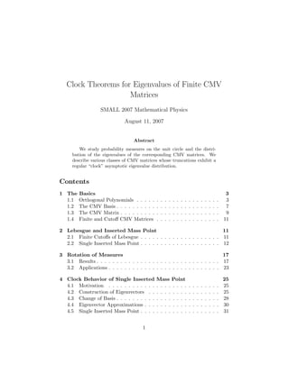
So let us look at some graphs to see what we expect to happen.
Let µ0 = (1−γ)λ+γδ1 and let S = C(dµ0). Then we know from Theorem
2.3 that the eigenvalues of S
(n)
1 are the nth roots of unity regardless of the
value of γ. So in order to determine what to expect in the very opposite
case, let us consider S
(n)
−1 . Figure 4.1 shows the similarities that most of
the eigenvalues of S
(n)
−1 have for one specific case. As we can see, only the
eigenvalues which are closest to the inserted mass are significantly perturbed
from the eigenvalues of the free matrix counterpart.
In general, only the eigenvalues which are closest to the mass point show
significant perturbation from the expected clock points. We would like to
determine exactly how far away from the clock points the eigenvalues are
and, if possible, show exactly the relationship with the clock points as n
grows without bound.
4.2 Construction of Eigenvectors
In order to determine the exact behavior of the eigenvalues of the finite
matrices associated with µ, we will have to examine the eigenvectors to
which they are associated. When looking at the finite matrix, it is not
easy to determine what the eigenvectors are. However, when viewed as an
25
26. -1 -0.5 0.5 1
-1
-0.5
0.5
1
(a) Eigenvalues of Λ
(20)
−1
-1 -0.5 0.5 1
-1
-0.5
0.5
1
(b) Eigenvalues of S
(20)
−1 for γ = 1
2
Figure 1: Compared Eigenvalues
operator on L2(∂D, dµ) with the proper measure (the spectral measure of
the matrix), the operator corresponds simply to multiplication by z, and
eigenfunctions are much easier to determine.
First, let us prove the following lemma:
Lemma 4.1. Let µ = (1−γ)λ+γδ1 and let S = C(dµ). Now let µ
(n)
β be the
spectral measure of S
(n)
β . Then the paraorthognal polynomial Φn,β(z) = 0
almost everywhere in L2(∂D, dµ
(n)
β ).
Proof. We know from [4] that Φn,β(z) is the characteristic polynomial of
S
(n)
β . This implies that Φn,β(S
(n)
β ) = 0. Define Mz : L2(∂D, dµ
(n)
β ) →
L2(∂D, dµ
(n)
β ) by Mz : f(z) → zf(z). By the spectral theorem, we know that
Φn,β(Mz) = 0. We know, however, that Φn,β(Mz)(f(z)) = Φn,β(z)f(z) = 0
∀f ∈ L2(∂D, dµ
(n)
β ). Hence Φn,β(z) = 0 almost everywhere.
This will give us the tools that we need in order to find the form of the
eigenvectors.
Lemma 4.2. Let Φn,β(z) = n
j=0 ajzj and let λ be any zero of Φn,β(z). If
we define f(z) = n−1
k=0 bk(λ)zk where
bj(λ) = −
1
λj+1
j
k=0
akλk
for 0 ≤ j ≤ n − 2
26
27. and bn−1(λ) = 1, then Mz(f(z)) = λf(z) in L2(∂D, dµ
(n)
β ).
Proof. Let us determine what the form of Mz(f(z)) is. Because Φn,β is
monic, we know that an = 1. Hence
Mz(f(z)) = zf(z)
= z
n−1
j=0
bjzj
= bn−1(λ)zn
+
n−2
j=0
bj(λ)zj+1
= zn
+
n−2
j=0
bj(λ)zj+1
= zn
− Φn,β +
n−2
j=0
bj(λ)zj+1
= −
n−2
j=0
ajzj
+
n−2
j=0
bj(λ)zj+1
=
n−1
j=1
(bj−1(λ) − aj) zj
− a0.
We know that
−a0 = λ(−
1
λ
(a0))
= λb0(λ).
Furthermore if 1 ≤ j ≤ n − 2
bj−1(λ) − aj = −
1
λj
j−1
k=0
akλk
− aj
= −
1
λj
j
k=0
akλk
= λ −
1
λj+1
j
k=0
akλk
= λbj(λ).
27
28. Finally
bn−2(λ) − an−1 = −
1
λn−1
n−2
k=0
akλk
− an−1
= −
1
λn−1
n−1
k=0
akλk
= −
1
λn−1
(Φn,β(λ) − λn
)
= −
1
λn−1
(−λn
)
= λ
= λbn−1(λ)
Thus we have shown that Mz(f(z)) = λf(z).
Clearly it is possible to find an eigenvector such that b0(λ) = 1 as well.
Thus we have the following lemma as well.
Lemma 4.3. Let Φn,β(z) = n
j=0 ajzj and let λ be any zero of Φn,β(z). If
we define f(z) = n−1
j=0 bk(λ)zk where
bj(λ) = −
λ
a0
n
k=j
akλk−j
for 1 ≤ j ≤ n − 1
and b0(λ) = 1, then Mz(f(z)) = λf(z).
The proof of this is similar to the proof of Lemma 4.2 and will therefore
be omitted here.
4.3 Change of Basis
It will frequently be useful to consider changing basis from {1, z, z−1, z2, . . .}
to {χ0, χ1, χ2, . . .} since it is with respect to this orthonormal basis that a
CMV matrix is the representation of multiplication by z.
Since {χ0, χ1, χ2, . . .} is an orthonormal basis, we can easily write the
matrix for a change of basis into this basis in terms of inner products. Specif-
ically, the matrix representation of a change of basis from {1, z, z−1, z2, . . .}
28
29. is
χ0, 1 χ0, z χ0, z−1 · · ·
χ1, 1 χ1, z χ1, z−1 · · ·
χ2, 1 χ2, z χ2, z−1 · · ·
...
...
...
...
Because of the definition of χn, we know that this matrix is actually upper
triangular. So it is given by
χ0, 1 χ0, z χ0, z−1 χ0, z2 · · ·
0 χ1, z χ1, z−1 χ1, z2 · · ·
0 0 χ2, z−1 χ2, z2 · · ·
0 0 0 χ3, z2 · · ·
...
...
...
...
...
One final refinement that we can make to our understanding of this matrix
is to look at the terms on the main diagonal. We must consider even and
odd cases. If n = 2k, then we have
χ2k, z−k
= z−k
ϕ∗
2k, z−k
= ϕ∗
2k, 1
= z2k
, ϕ2k
=
1
Φ2k
z2k
, Φ2k
=
1
Φ2k
z2k
, P(z2k
)
where P is the orthogonal projection onto Span{1, z, z2, . . . , z2k−1}⊥. Since
projections have the property that P = P∗ = P2, we have the following:
χ2k, z−k
=
1
Φ2k
z2k
, P(z2k
)
=
1
Φ2k
P(z2k
), P(z2k
)
=
1
Φ2k
Φ2k, Φ2k
= Φ2k
A similar calculation shows that
χ2k−1, zk
= Φ2k−1
29
30. Hence the matrix form of the change of basis is
Φ0 χ0, z χ0, z−1 χ0, z2 · · ·
0 Φ1 χ1, z−1 χ1, z2 · · ·
0 0 Φ2 χ2, z2 · · ·
0 0 0 Φ3 · · ·
...
...
...
...
...
4.4 Eigenvector Approximations
While the formula for the eigenvectors presented in Section 4.2 is of little
use unless the eigenvalues are already known, a small modification provides
useful results.
Lemmas 4.2 and 4.3 provide formulas for the eigenvalues as functions of
λ, the zeroes of the paraorthogonal polynomial. A natrual question which
arises from this formula is the question of what happens when the λ used in
the formula is not a zero of the paraorthogonal polynomial. If λ is changed
only slightly from an eigenvalue, we expect to obtain something which is very
close to an eigenvector, even though it is clearly not actually an eigenvector.
The exploration of this question leads to the following lemma.
Lemma 4.4. Let Φn,β = n
k=0 ajzj be a paraorthogonal polynomial and let
λ ∈ ∂D. If f(z) = n−1
k=0 bk(λ)zk is defined as in Lemma 4.2 or 4.3, then
(Mz − λ)(f(z)) = |Φn,β(λ)|
Once again, we will prove this for coefficients as defined in Lemma 4.2
and omit the proof for coefficients as defined in Lemma 4.3 as the proofs are
very similar.
Proof. As shown in Lemma 4.2,
Mz(f(z)) = zf(z)
=
n−1
k=1
(bk−1 − ak) − a0.
Hence we have
(Mz − λ)(f(z)) =
n−1
k=1
(bk−1 − ak − λbk) − (a0 + λb0)
=
n−1
k=1
(bk−1 − ak − λbk)
30
31. since b0 = −a0
λ . Examining the other terms, we get for 1 ≤ k ≤ n − 2
bk−1 − ak − λbk = −
1
λk
k−1
j=0
akλk
− ak − λbk
= −
1
λk
k
j=0
akλk
− λbk
= λbk − λbk
= 0.
Finally
bn−2 − an−1 − λbn−1 = bn−2 − an−1 − λ
= −
1
λn−1
n−2
k=0
akλk
− an−1 − λ
= −
1
λn−1
n−1
k=0
akλk
− λan
= −
1
λn−1
n
k=0
akλk
= −
1
λn−1
Φn,β(λ)
Hence
(Mz − λ)(f(z)) = −
1
λn−1
Φn,β(λ)zn−1
.
Thus
(Mz − λ)(f(z)) = |Φn,β(λ)|
as desired.
This is only one step on the way to finding eigenvalues of finite matrices
due to the fact that we know nothing about the norm of f(z). But it will
be enough to tell us something about the eigenvalues of the case when we
are looking at the single inserted mass point measure.
4.5 Single Inserted Mass Point
It is at this point that we will turn to a specific example. Once again we
will let µ = (1 − γ)λ + γδ1 and S = C(dµ). First we will want to determine
31
32. Φn,β. Theorem 2.2 gives us
Φn−1(z) = zn−1
−
γ
1 + nγ − 2γ
n−2
k=0
zk
.
Hence
Φ∗
n−1(z) = 1 −
γ
1 + nγ − 2γ
n−1
k=1
zk
.
Therefore we conclude that
Φn,β(z) = zΦn−1 − βΦ∗
n−1
= zn
−
γ
1 + nγ − 2γ
n−1
k=1
zk
+
βγ
1 + nγ − 2γ
n−1
k=1
zk
− β
= zn
+
γ(β − 1)
1 + nγ − 2γ
n−1
k=1
zk
− β.
Now it is our guess that the zeroes of this polynomial are close to nth
roots of β. So let λ ∈ ∂D such that λn = β. Then we have
Φn,β(λ) = λn
−
γ(β − 1)
1 + nγ − 2γ
n−1
k=1
λk
− β
=
γ(β − 1)
1 + nγ − 2γ
n−1
k=1
λk
=
γ(β − 1)
1 + nγ − 2γ
λn − λ
λ − 1
.
Knowing that |λn − λ| ≤ 2 and |β − 1| ≤ 2 since λ, β ∈ ∂D, we thus have
that
|Φn,β(λ)| ≤
4γ
(λ − 1)(1 + nγ − 2γ)
. (4.1)
We will now wish to find an estimate for how far away from an eigenvalue
this is. We have
(Mz − λ)(f(z)) ≤
4γ
(λ − 1)(1 + nγ − 2γ)
.
So we need to estimate f(z) . An estimate for this norm is not immediately
forthcoming, but an extremely poor estimate presents itself if we consider
32
33. that we can write f(z) in the χ basis using the change of basis matrix
presented in section 4.3.
Writing f(z) in the form that we have it in the basis {1, z, z−1, z2, . . .}
is not particularly easy, but note that
Mz − λ)(f(z)) = (Mz − λ)(zq
f(z))
for any q since multiplication by z is unitary. Hence we can simply use a
different function which is much more easily written in the preferred basis
without destroying the information that we worked so hard to obtain. De-
pending on the parity of n, either the leading term or the constant term will
become the coefficient of the last power of z in {1, z, z−1, z2, . . .}. Hence if
n is even, we will use the form of the approximate eiegenvector presented in
Lemma 4.2 and if n is odd, we will use Lemma 4.3.
The important fact here is that the last row of the change of basis matrix
only has one term in it, hence we know that
zq
f(z) = Φn−1(z) χn−1 + · · ·
if we change basis to {χ0, χ1, . . . , χn−1}. Furthermore since this is an or-
thonormal basis, we know that
f(z) ≥ Φn−1(z) .
Thus if we can approximate this, we have a lower bound for the norm in
which we are interested. So we have the following lemma:
Lemma 4.5. If {Φn}n≥0 are the monic orthogonal polynomials associated
with µ = (1 − γ)λ + γδ1, then
Φn ≥ 1 − γ, ∀n ≥ 0.
Proof. We know from 1.13 that
Φn =
n−1
k=0
ρk
=
n−1
k=0
1 − |αk|2.
So
lim
n→∞
Φn =
∞
k=0
ρk.
33
34. Hence we have
log lim
n→∞
Φn =
∞
k=0
log ρk
=
1
2
∞
k=0
log 1 − |αk|2
.
Since |αk|2 < 1, we know that log 1 − |αk|2 = − ∞
j=1
1
j |αk|2j. Hence
log lim
n→∞
Φn = −
1
2
∞
k=0
∞
j=1
1
j
|αk|2j
= −
∞
j=1
1
2j
∞
k=0
|αk|2j
.
Examining the inner sum, Theorem 2.2 and Abel’s Summation Formula give
us
0≤k<x
|αk|2j
=
0≤k<x
1
γ−1 + k
2j
=
x + 1
(γ−1 + t)2j
+ 2j
x
0
t + 1
(γ−1 + t)2j+1
dt.
Hence since 2j > 1 for all j ≥ 1, we have
∞
k=0
|αk|2j
= 2j
∞
0
t + 1
(γ−1 + t)2j+1
dt
= 2j
∞
γ−1
u − γ−1 + 1
u2j+1
du
≤ 2j
∞
γ−1
u − γ−1 + 1
u2j+1
du
≤ 2j
∞
γ−1
u + 1
u2j+1
du
= 2j
∞
γ−1
u−2j
+ u−2j−1
du
= 2j −
1
2j − 1
u−2j+1
−
1
2j
u−2j
∞
γ−1
= 2j
γ2j−1
2j − 1
+
γ2j
2j
.
34
35. Hence we have
log lim
n→∞
Φn ≥ −
∞
j=1
1
2j
2j
γ2j−1
2j − 1
+
γ2j
2j
= −
∞
m=1
γm
m
.
But since |γ| < 1, this gives us
log lim
n→∞
Φn ≥ log (1 − γ) .
Hence
lim
n→∞
Φn ≥ 1 − γ.
But since Φn
Φn−1
= ρn−1 and ρn−1 < 1, this means that { Φn }∞
n=0 is a
strictly decreasing sequence of real numbers, hence
Φn ≥ 1 − γ, ∀n ≥ 0
as desired.
And with that, we get the following estimate:
(Mz − λ)
f(z)
f(z)
≤
4γ
(1 − γ)(λ − 1)(1 + nγ − 2γ)
Since f(z)
f(z) is a unit vector, we therefore know that there is an eigenvalue
λ such that
|λ − λ| ≤
4γ
(1 − γ)(λ − 1)(1 + nγ − 2γ)
5 “Almost Free” CMV Matrices
5.1 A Review of Clock Theorems
We conjectured in Section 4 that most of the zeros of Φn,β for inserted mass
point converge to roots of β as n → ∞. In particular, this would mean that
the distance between neighboring zeros would converge to 2π/n. This last
condition is called clock behavior. We will now state some known results
concerning this behavior to help put our result into context.
35
36. Theorem 5.1 (Theorem 4.1 of [7]). Let {αj}j≥0 be a sequence of Verblunsky
coefficients satisfying
∞
j=0
|αj| < ∞ (5.1)
and let {βj}j≥1 be a sequence of points on ∂D. Let {θ
(n)
j }n
j=1 be defined
so 0 ≤ θ
(n)
1 ≤ · · · ≤ θ
(n)
n < 2π and so that eiθ
(n)
j are the zeros of the
paraorthogonal polynomials Φn,βj
. Then (with θ
(n)
n+1 ≡ θ
(n)+2π
1 )
sup
j
n θ
(n)
j+1 − θ
(n)
j −
2π
n
→ 0
as n → ∞.
This result does not apply to inserted mass point; in that case there
exists C such that |αn| ≥ C/n ∀n and hence
∞
n=0
|αn| ≥
∞
n=0
C
n
= ∞.
Theorem 5.2 (Theorem 1.7 in [1]). If E{|αk|2} = o(k−1), then (with prob-
ability 1) the spacing between eigenvalues converges to 2π/n.
Inserted mass point satisfies the hypothesis of this theorem since we can
pick C such that |αk| ≤ C/k ∀k and get
lim
k→∞
|αk|2
k−1
≤ lim
k→∞
C2
k
= 0.
This puts inserted mass point in an interesting position; while Theorem
5.2 tells us that we should expect clock behavior, this is not guaranteed by
Theorem 5.1. Indeed, Simon conjectures in [7] that Theorem 5.1 stills holds
if |αn| = C0n−1 + error with either error ∈ 1 or |error| ≤ Cn−2.
5.2 Shifted CMV Matrices
One interesting property of inserted mass point is that if we shift the Verblun-
sky coefficients we get Verblunsky coefficients for a different inserted mass
point:
36
37. Lemma 5.3. Let αk(ω, γ) = αk(µω,γ). Then for any n and m we have
αn+m(ω, γ) = αn(ω−m
, (1/γ + m)−1
). (5.2)
Proof.
αn+m(ω, γ) =
ω−(n+m+1)
1/γ + n + m
=
(ω−m)−(n+1)
(1/γ + m) + n
= αn(ω−m
, (1/γ + m)−1
).
Since
lim
m→∞
(1/γ + m)−1
γ
= lim
m→∞
1
1 + γm
= 0
we see that increasing m will make γ arbitrarily small, in some sense bringing
us closer to Lebesgue measure. This motivates the following definitions:
Definition 5.4 (Shifted CMV Matrix). For a CMV matrix C = C(α0, α1, . . .)
and β ∈ ∂D define the shifted CMV matrix C
(n,m)
β by
C
(n,m)
β = C(αm, αm+1, . . . , αn−2, β). (5.3)
Definition 5.5. Let C = C(α0, α1, . . .) be a CMV matrix. Define functions
d and by
d(n, m) = max
i
min
j
|λi − µj|, (n, m) = min
i=j
|λi − λj|.
where {µi} are the eigenvalues of C
(n,m)
β and {λi} the eigenvalues of Λ
(n−m)
β .
Definition 5.6 (Almost Free). Let C = C(α0, α1, . . .) be a CMV matrix. If
for all > 0 there exists N such that for all n > N there is an mn satisfying
d(n, mn) < (n, mn) and
lim
n→∞
mn
n
= 0
we say that C is almost free.
Lemma 5.7. For m < n and n ≥ 2 we have
(n, m) ≥ 2 sin(π
n ) ≥ 4n−1
. (5.4)
37
38. Proof. Note that, since the eigenvalues of Λ
(n−m)
β are solutions of zn−m − β,
the distance between any two neighboring eigenvalues will be
(n, m) = |ei 2π
n−m − 1| = 2 − 2 cos 2π
n−m
= 4 sin2 π
n−m = 2 sin( π
n−m)
≥ 2 sin(π
n ).
Since sin θ is concave down on (0, π/2) we have have sin θ ≥ 2
π θ for any θ ∈
(0, π/2), so in particular if n ≥ 2 we have sin(π/n) ≥ (2/π)(π/n) = 2/n.
5.3 Norm Estimates
In this section we find sufficient conditions on Verblunsky coefficients for a
CMV matrix to be almost free.
Definition 5.8. For A an n × n matrix with ijth entry aij, define A 2 by
A 2 =
n
i=1
n
j=1
|aij|2
1/2
(5.5)
Lemma 5.9. For any n × n matrix A, A ≤ A 2.
Proof. Let aij be the ijth entry of A and let ai be its ith row. If x =
(x0, x1, . . . , xn) ∈ Cn satisfies x = 1 then
Ax 2
=
n
i=1
n
j=1
aijxj
2
=
n
i=1
| ai, x |2
≤
n
i=1
ai
2
= A 2
2 .
Lemma 5.10. Let A be a normal n × n matrix with eigenvalues λ1, . . . , λn.
Then A = max
i
|λi|.
Proof. Since A is normal there exists an orthonormal basis of eigenvectors
e1, . . . , en corresponding to eigenvalues λ1, . . . , λn. Let x = n
i=1 αiei satisfy
x = 1. Then
Ax 2
= A
n
i=1
αiei
2
=
n
i=1
αiλiei
2
=
n
i=1
|αi|2
|λi|2
≤
n
i=1
|αi|2
max
j
|λj|
2
= max
j
|λj|
2
.
38
39. To show the other inequality let λk be the eigenvalue of A with maximal
absolute value. Then Aek = λkek =⇒ Aek = |λk| =⇒ A ≥ |λk|.
Lemma 5.11. Let A be a normal n × n matrix and B an arbitrary n × n
matrix. If A − B < for some > 0, then for any eigenvalue λ of B
there exists an eigenvalue µ of A such that |λ − µ| < .
Proof. If λ is an eigenvalue of A then we’re done, so assume that λ is not
an eigenvalue of A, i.e. that A − λI is invertible. Since λ is an eigenvalue of
B there must exist some w ∈ Cn such that Bw = λw. This gives
w > (A − B)w = Aw − λw = (A − λI)w .
Now we set v = (A − λI)w and observe that the above inequality becomes
(A − λI)−1
v > (A − λI)(A − λI)−1
v
(A − λ)−1
v >
1
v
which implies (A − λ)−1 > 1/ , and hence by Lemma 5.10 that (A−λ)−1
must have at least one eigenvalue µ satisfying |µ| > 1/ . Thus A − λI has
µ−1 as an eigenvalue for some eigenvector y and we get
(A − λI)y = µ−1
y
Ay = (µ−1
+ λ)y.
Therefore µ = µ−1+λ is an eigenvalue of A satisfying |µ−λ| = |µ−1| < .
Theorem 5.12. Let C = C(α0, α1, . . .) be a CMV matrix and fix β ∈ ∂D.
Then
C
(n)
β − Λ
(n)
β
2
≤ 4
n−2
k=m
|αk|2
. (5.6)
Remark. Simon [6] gives a much more general estimate for infinite CMV
matrices using the LM factorization, which in our case reduces to
C
(n)
β − Λ
(n)
β
2
≤ 12
∞
k=0
1 − 1 − |αk|2 .
39
40. Proof. We will first find C
(n)
β − Λ
(n)
β
2
2 and then apply Lemma 5.9. To
simplify computation, define the following sequences to the five diagonals of
C
(n)
β −Λ
(n)
β omitting both the first terms of each diagonal and those involving
β (d0 is the main diagonal, d1 the first diagonal above it, etc):
d0 = −α1α0, −α2α1, −α3α2, . . .
d1 = −ρ1α0, α3ρ2, −ρ3α2, α5ρ4, −ρ5α4, . . .
d−1 = α2ρ1, −ρ2α1, α4ρ3, −ρ4α3, α6ρ5, . . .
d2 = 0, ρ3ρ2 − 1, 0, ρ5ρ4 − 1, 0, ρ7ρ6 − 1, . . .
d−2 = ρ2ρ1 − 1, 0, ρ4ρ3 − 1, 0, ρ6ρ5 − 1, 0, . . .
From the main diagonal, we get
n−2
k=1
|d0(k)|2
=
n−2
k=1
| − αkαk−1|2
=
n−2
k=1
|αkαk−1|2
.
Combining d1 and d−1 we get two new sums
n−2
k=1
| − ρkαk−1|2
+
n−3
k=1
|αk+1ρk|2
.
Since the (n−2)th term involves β, the second sum only goes up to k = n−3.
The first sum yields
n−2
k=1
| − ρkαk−2|2
=
n−2
k=1
|αk−1|2
(1 − |αk|2
) =
n−2
k=1
|αk−1|2
− |αk−2|2
|αk|2
=
n−2
k=1
|αk−1|2
−
n−2
k=1
|αk−1αk|2
and for the second we get
n−3
k=1
|αk+1ρk|2
=
n−3
k=1
|αk+1|2
(1 − |αk|2
) =
n−3
k=1
|αk+1|2
− |αk+1|2
|αk|2
=
n−3
k=1
|αk+1|2
−
n−3
k=1
|αkαk+1|2
.
40
41. Combining d2 and d−2 we get
n−3
k=1
(1 − ρkρk+1)2
=
n−3
k=1
(1 − 2ρkρk+1 + ρ2
kρ2
k+1)
=
n−3
k=1
1 − 2ρkρk+1 + (1 − |αk|2
)(1 − |αk+1|2
)
=
n−3
k=1
2(1 − ρkρk+1) + |αkαk+1|2
− |αk|2
− |αk+1|2
which gives us four sums:
2
n−3
k=1
(1 − ρkρk+1) +
n−3
k=1
|αkαk+1|2
−
n−3
k=1
|αk|2
−
n−3
k=1
|αk+1|2
.
Since xy ≤ x2 +y2 for x, y ≥ 0, we can get a simple bound for the first term:
2
n−3
k=1
(1 − ρkρk+1) ≤ 2
n−3
k=1
1 − ρ2
k + 1 − ρ2
k+1
= 2
n−3
k=1
|αk|2
+ 2
n−3
k=1
|αk+1|2
.
The first entries of the diagonals contribute
|α0|2
+ |ρ0α1|2
+ |ρ0 − 1|2
≤ |α0|2
+ (1 − |α0|2
)|α1|2
+ |ρ2
0 − 1|2
= |α0|2
+ |α1|2
− |α0α1|2
− |α0|4
and the terms with β will give
|βρn−2 − β|2
+ |βαn−2|2
= (ρn−2 − 1)2
+ |αn−2|2
≤ (ρ2
n−2 − 1)2
+ |αn−2|2
= |αn−2|4
+ |αn−2|2
.
Note that all of the sums involving |αkαk+1|2 cancel. Reindexing sums
involving |αk|2 we see that they add up to
4
n−3
k=2
|αk|2
+ |α0|2
+ 2|α1|2
+ 2|αn−2|2
.
41
42. Adding the first entries of the diagonals and those involving β we get
4
n−3
k=2
|αk|2
+ 2|α0|2
+ 3|α1|2
+ 3|αn−2|2
+ |αn−2|4
− |α0α1|2
− |α0|4
which is less than or equal to (throwing out negative terms and replacing
|αn−1|4 with |αn−1|2)
4
n−3
k=2
|αk|2
+ 2|α0|2
+ 3|α1|2
+ 4|αn−2|2
≤ 4
n−2
k=0
|αk|2
.
Thus by Lemma 5.9 we have
C
(n)
β − Λ
(n)
β
2
≤ 4
n−2
k=0
|αk|2
as desired.
Corollary 5.13. For every eigenvalue λ of Λ
(n−m)
β there exists an eigenvalue
µ of C
(n,m)
β such that
|µ − λ|2
≤ 4
n−2
k=m
|αk|2
. (5.7)
Equivalently we have
d(n, m)2
≤ 4
n−2
k=m
|αk|2
. (5.8)
Proof. This follows directly from Theorem 5.12 and Lemma 5.11.
5.4 Necessary Conditions
Example 5.14. We will show that the CMV matrix for the Rogers-Szeg˝o
polynomials is almost free. For some q ∈ (0, 1) the Rogers-Szeg˝o polynomials
are the orthogonal polynomials for the measure
dµ(θ) = (2π log(1/q))−1/2
∞
j=−∞
q−(θ−2πj)2/2
dθ
42
43. with Verblunsky coefficients αk = (−1)kq(k+1)/2.
Then
n−1
k=m
|αk|2
=
n−1
k=m
qm+1
=
qm+1 − qn+1
1 − q
≤
qm
1 − q
(5.9)
which, by Corollary 5.13, means that d(n, m)2 ≤ 4qm/(1 − q). With con-
stants r ∈ (0, 1) and K where
r =
√
q, K = 4/(1 − q) (5.10)
this relation becomes
d(n, m) ≤ Krm
. (5.11)
Given > 0 we want to find the smallest possible m satisfying d(n, m) <
(n, m). Using Lemma 5.7 we see that
Krm
<
4
n
(5.12)
is sufficient. Since both sides of this inequality are strictly positive, we can
take their logarithms to get
m log r + log K < log(4 /n) (5.13)
m >
log((4 /K)n−1)
log r
(5.14)
=
log[K/(4 )] + log n
log(1/r)
(5.15)
where all of the terms except perhaps log[K/(2 )] are now positive. Thus
m = mn =
log[K/(4 )] + log n
log(1/r)
(5.16)
guarantees (5.12). Clearly
lim
n→∞
mn
n
= lim
n→∞
1
n
log[K/(4 )] + log n
log(1/r)
= 0. (5.17)
This also implies that certainly mn < n − 1 for all sufficiently large n.
Now we use Corollary 5.13 to show to that a much broader category of
CMV matrices are almost free:
43
44. Theorem 5.15. Let C = C(α0, α1, . . .) be a CMV matrix. If
∞
k=m
|αk|2
≤
M
mγ
(5.18)
for some γ > 2 and M > 0, then C is almost free.
Proof. Fix > 0. If we let K = 2
√
M and β = γ/2 then by Corollary 5.13
we have d(n, m) ≤ K/mβ. By Lemma 5.7 we need only can find m < n − 1
such that
K
mβ
<
4
n
(5.19)
to guarantee d(n, m) < ( (n, m)). Solving for m, this inequality becomes
m >
Kn
4
1/β
. (5.20)
Thus choosing
mn =
Kn
4
1/β
(5.21)
will satisfy (5.19). Of course we may not have mn < n − 1 for some n.
However,
lim
n→∞
mn
n
= lim
n→∞
1
n
Kn
4
1/β
(5.22)
≤ lim
n→∞
1
n
K
4
1/β
n1/β
+ 1 (5.23)
=
K
4
1/β
lim
n→∞
n1/β−1
+ lim
n→∞
1
n
(5.24)
= 0 (5.25)
(since 1/β − 1 < 0); thus we must have mn < n − 1 for all n sufficiently
large.
Theorem 5.16. Let dµ = w(θ)dθ
2π with weight function w(θ) > 0, infθ w(θ) =
α > 0, and |ci(dµ)| < ∞. Then
sup β
∞
n=1
(1 + |n|)β
|cn(dµ)| < ∞ = sup β
∞
n=1
(1 + |n|)β
|αn(dµ)| < ∞
44
45. Remark. This is stated in Simon [4] as an immediate consequence of the
extended Baxter’s theorem, and will not be proved here.
Theorem 5.17. Assume that there exist p > 1 and M > 0 such that, for
all n > 0, |cn| < M/np. Then for all ∈ (0, 1) there exists K such that
∞
n=m
|αn|2
≤
K
m2(p−1)−
. (5.26)
Proof. We know from Theorem 5.16 that
c = sup β
∞
n=0
(1 + n)β
|αn| < ∞ = sup β
∞
n=0
(1 + n)β
|cn| < ∞ ,
(5.27)
and since |cn| ≤ M/np ∀n > 0 we have
∞
n=0
(1 + n)β
|cn| ≤ |c0| + M
∞
n=1
(1 + n)β
np
(5.28)
≤ 1 + M
∞
n=1
(2n)β
np
(5.29)
= 1 + 2β
M
∞
n=1
1
np−β
(5.30)
which converges for p − β > 1 =⇒ β < p − 1. Therefore c ≥ p − 1 and we
have that for all 1 ∈ (0, 1)
∞
n=0
(1 + n)p−1− 1
|αn| < ∞. (5.31)
For convenience let q = p − 1 − 1. Now for any m ∈ N we have
∞
n=0
(1 + n)q
|αn| =
m−1
n=0
(1 + n)q
|αn| +
∞
n=m
(1 + n)q
|αn|
45
47. and hence
lim
m→∞
m2(p−1)−
∞
n=m
|αn|2
= 0.
This tells us that there exists N such that for all m > N
m2(p−1)−
∞
n=m
|αn|2
< 1
or equivalently
∞
n=m
|αn|2
<
1
m2(p−1)−
.
Let
S = max
m≤N
∞
n=m
|αn|2
and choose K such that K/N2(p−1)− > S. Then we have that, for all
m ≤ N,
∞
n=m
|αn|2
<
K
m2(p−1)−
.
With K = max(K, 1) we have that for all m
∞
n=m
|αn|2
<
K
m2(p−1)−
as desired.
Remark. We would like to thank Tim Heath for helping us with the proof
of Theorem 5.17.
Corollary 5.18. Let C be a CMV matrix whose moments satisfy the hy-
pothesis of Theorem 5.17 for p > 2. Then C is almost free.
Proof. By Theorem 5.17 we know that for any ∈ (0, 1) there exists K such
that
∞
n=m
|αn|2
<
K
m2(p−1)−
. (5.32)
In particular we can choose such that 2(p − 1) − > 2. Then by Theorem
5.15 C is almost free.
47
48. Lemma 5.19. Let f : [0, 2π] → (0, ∞) be an r times differentiable function
with bounded rth derivative, say |fr(θ)| < M for all θ, and fk(0) = fk(2π)
for k < r − 1. Then there exists K such that for all n > 0
2π
0
e−inθ
f(θ) dt ≤
K
nr
. (5.33)
Proof. If r = 0 then we have
2π
0
e−inθ
f(θ) dθ ≤
2π
0
|e−inθ
f(θ)| dθ ≤ 2πM =
2πM
n0
.
Assume then that Lemma 5.19 holds for r = k and let f satisfy the hypoth-
esis of Lemma 5.19 for r = k + 1. Using integration by parts we get
2π
0
e−inθ
f(θ) dθ =
e−inθf(θ)
−in
2π
0
+
1
in
2π
0
e−inθ
f (θ) dθ
=
1
in
2π
0
e−inθ
f (θ) dθ.
Now f satisfies the hypothesis of Lemma 5.19 for r = k, so there exists K
such that
2π
0
e−inθ
f (θ) dt ≤
K
nk
.
This gives
2π
0
e−inθ
f(θ) dθ =
1
n
2π
0
e−inθ
f (θ) dt ≤
1
n
K
nk
=
K
nk+1
.
Theorem 5.20. Let f : [0, 2π] → (0, ∞) satisfy the hypothesis of Lemma
5.19 for some r > 2. If
2π
0 f(θ)dθ = 2π then dµ(θ) = f(θ)dθ
2π is a nontrivial
probability measure whose CMV matrix is almost free.
Proof. That dµ is a nontrivial probability measure is clear from the condi-
tions on f. Using the K given by Lemma 5.19 we get
|cn| =
1
2π
2π
0
e−inθ
f(θ) dθ ≤
K/2π
nr
and hence by Corollary 5.18 that the CMV matrix for dµ is almost free.
48
49. Remark. It is important to note that Theorem 5.1 more or less implies
Theorem 5.15: Let γ > 2. If
∞
k=m
|αk|2
≤
M
mγ
then we must also have |αm| ≤ M/mγ. This gives
∞
k=0
|αk| =
∞
k=0
M
kγ
< ∞
and hence by Theorem 5.1 that the distance between neighboring eigenvalues
of C
(n)
β = C
(n,0)
β approaches 2π/n and hence that they will converge to the
eigenvalues of Λ
(n)
β for some β ∈ ∂D. The only technicality is that we may
not have β = β.
5.5 Properties of Almost Free CMV Matrices
In this section we’ll investigate the properties of almost free CMV matrices,
in particular how the eigenvalues of their finite CMV matrices compare to
the those of the free CMV matrix of the same dimension. In order to do
this, we’ll need several facts from [4].
Lemma 5.21. Let C = C(α0, α1, . . .) be a matrix. Then for all n and m < n
there exists a rank one matrix Q and a unitary m × m matrix K such that
C
(n)
β − Q = K ⊕ B (5.34)
where B = C
(n,m)
β if m is even and (C
(n,m)
β ) if m is odd.
Remark. This is a less general version of Theorem 4.5.2 of [4].
Proof. Just as with full CMV matrices, we can write C = LM with L and
M defined as in (1.30) and (1.31). If m is even, let M be M with Θm−1
replaced by β 0
0 1
with β = (1 + αm−1)/(1 + αm). It’s straightforward to
check that M−M has rank 1 and hence that L(M−M ) has rank at most
1. Setting Q = L(M − M ) we see that C − Q = LM has the desired form.
A similar argument involving modifying L works for n odd.
Lemma 5.22. Let U and V be two n × n unitary matrices such that U − V
is rank 1 and denote the number of eigenvalues of the matrix A contained
49
50. in the set D by ED(A). If I = {eiθ : |θ − θ0| < δ} for some θ0 ∈ [0, 2π] and
δ < π then
|EI(U) − EI(V )| ≤ 1. (5.35)
Remark. This is an immediate consequence of Equation 1.4.25 of [4].
Theorem 5.23. Let C be an almost free CMV matrix and fix β ∈ ∂D. For
> 0 pick n and m such that d(n, m) < (n, m). Let {λi} be the eigenvalues
of Λ
(n−m)
β . Pick {θ1, . . . , θk} such that λk = eiθk . Then for all but at most
m intervals of the form
Ik = eiθ
: θ ∈ (θk − 2π
n−m, θk+1 + 2π
n−m)
contain an eigenvalue of C
(n)
β .
Proof. First we’ll show that EIk
(C
(n,m)
β ) ≥ 2 for all k. Define
φd(n, m) = max
i
min
j
|λi − µj| (5.36)
φ (n, m) = min
i=j
|λi − λj| = 2π
n−m. (5.37)
Then d(n, m) < (n, m) implies φd(n, m) < φ (n, m), so for each eigenvalue
eiθk of Λ
(m)
β there exists an eigenvalue eiφk of C
(n,m)
β such that |φk − θk| <
2π
n−m. This gives eiφk , eiφk+1 ∈ Ik and hence EIk
(C
(n,m)
β ) ≥ 2 as desired.
Lemmas 5.21 and 5.22 give
EIk
(C
(n)
β ) − EIk
(K ⊕ B) ≤ 1. (5.38)
Since EIk
(K ⊕ C
(n,m)
β ) = EIk
(K) + EIk
(B) this becomes
EIk
(C
(n)
β ) − EIk
(K) − EIk
(B) ≤ 1. (5.39)
Since K is an m × m matrix it has at most m eigenvalues. Hence for all but
at most m of the Ik we’ll have EIk
(K) = 0 and therefore
EIk
(C
(n)
β ) − EIk
(B) ≤ 1. (5.40)
Since EIk
(B) = EIk
(C
(n,m)
β ) (because the eigenvalues of a matrix A and its
transpose are the same) we have EIk
(B) ≥ 2 and hence
EIk
(C
(n)
β ) ≥ 1. (5.41)
50
51. Remark. Simon proves a very similar theorem about the interlacing of the
zeros of paraorthogonal polynomials in [8].
References
[1] Rowan Killip and Mihai Stoiciu. Eigenvalue statistics for cmv matrices:
From poisson to clock via circular beta ensembles, preprint. Available
at arXiv:math-ph/0608002v1.
[2] Steven J. Leon. Linear algebra with applications. Macmillan Inc., New
York, 1980.
[3] Barry Simon. Orthogonal polynomials on the unit circle: new results.
Int. Math. Res. Not., (53):2837–2880, 2004.
[4] Barry Simon. Orthogonal polynomials on the unit circle. Part 1, vol-
ume 54 of American Mathematical Society Colloquium Publications.
American Mathematical Society, Providence, RI, 2005. Classical the-
ory.
[5] Barry Simon. Orthogonal polynomials on the unit circle. Part 2, vol-
ume 54 of American Mathematical Society Colloquium Publications.
American Mathematical Society, Providence, RI, 2005. Spectral theory.
[6] Barry Simon. CMV matrices: Five years after. ArXiv Mathematics
e-prints, March 2006.
[7] Barry Simon. Fine structure of the zeros of orthogonal polynomials.
I. A tale of two pictures. Electron. Trans. Numer. Anal., 25:328–368
(electronic), 2006.
[8] Barry Simon. Rank one perturbations and the zeros of paraorthogonal
polynomials on the unit circle. J. Math. Anal. Appl., 329(1):376–382,
2007.
[9] Gerald Teschl. Functional analysis. Available at
http://www.mat.univie.ac.at/~gerald/ftp/book-fa/index.html.
51