Javier Garcia - Verdugo Sanchez - Six Sigma Training - W2 T- Test

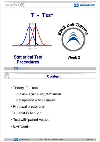
T - TestT Test
δδ
1x 2x
Statistical Test
Procedures
Week 2
Knorr-Bremse Group
Procedures
Content
Theory T test• Theory T – test
• Sample against long term meanSample against long term mean
• Comparison of two samples
• Practical procedure
• T – test in Minitab
• Test with paired values
Exercises• Exercises
Knorr-Bremse Group 03 BB W2 T-Test 08, D. Szemkus/H. Winkler Page 2/28

About the T-Test
We apply the T- test to determine if maximal two sets ofpp y
data belong to the same population or not.
Requirements:Requirements:
• Comparison of two independent group mean values
• Values are normal distributed
• Equal variation
Validation of Factors Y = f(x)
Factor X = Input
Part of the
Green Belt p
Discrete / Attributive Continuous / Variable
Green Belt
Training
tput
screte
ibutive
Chi-Square
Logistic
Regression
Y=Out
Dis
Attr
Regression
ResultY
nuous
able
T - Test
Regression
R
Contin
Varia
ANOVA ( F - Test)
Variance Test
Regression
Statistical techniques for all combination of data types are available
Statistical techniques for all combination of data types are available

T-Values
• T values are used for the estimation of the magnitude
of an effect (Is the effect significant?). An effect is( g )
defined as the difference of two mean values.
The units of T values are in standard errors E g a T• The units of T-values are in standard errors. E.g., a T-
value of +2,00 says, that the effect is 2 standard errors
away from 0 00 (or from a target value)away from 0,00 (or from a target value).
In Minitab:In Minitab:
• Every T-value is connected with a probability (the P-
value).
• E g a T value of 1 97 correlates to a p value of 0 085• E.g. a T-value of -1,97 correlates to a p-value of 0,085.
This means, that the probability to get T-values of -
1 97or less is 8 5%
1,97or less is 8,5%.
T – Test for a Sample
Test distribution and critical area for n = 10 and α = 0,05
1- α = 0 95025,0=
α
025,0=
α
432101234
1- α = 0.95,
2
,
2
43210-1-2-3-4
Tcrit = -2,26 Tcrit = 2,26
H0
don’t reject rejectreject
H0H0

Critical T-Values
11 - α
eedom
Degrees of freedom
esoffre
For one sample n – 1
Degree
For two samples
n1 + n2 - 2n1 + n2 2
An Example
A product line manufactures plates whit a target value (long term
mean) for thickness of µ = 0,25 cm.) µ ,
To proof this we measure 10 samples:
Mean = 0,253 cm und StDev = 0,03
s
X
T
µ−
=
T = calculated T-value of the sample
X = Mean of the sample
n
s µ = LT mean or target value
S = Standard deviation of the sample
n n = Sample size
Is the machine still performing accurate?
Critical T-value from the page before = 2,26

T – Test for Two Samples
XX
Possibility 1: The sample size for both samples are equal
2
=T 2
2
2
1
21
ss
XX
+
−
2
21
n
Possibility 2: The sample size for both samples are not equal
( ) ( )11 2
2
2
2
1
1 −+−
=
snsn
s
21 XX
T
−
=
221
−+ nn
21
21
nn
nn
s
+
21
Here we need the pooled standard deviation
Here we need the pooled standard deviation.
An Example
Let´s assume the output (Y) we measure is a metric for the surface quality
of laminate. We want to figure out if the yield of the modified (New) process
has been significantly improved compared to the current (Old) processhas been significantly improved compared to the current (Old) process.
The data of the investigation are shown below. The values in (%) are the
results of 48 sheets cut into 288 panels per experimental runresults of 48 sheets cut into 288 panels per experimental run.
“Old” “New”
89.7 84.7
81.4 86.1
84 5 83 2 How would you formulate HHow would you formulate H84.5 83.2
84.8 91.9
87.3 86.3
How would you formulate Ho
and Ha for this example?
How would you formulate Ho
and Ha for this example?
79.7 79.3
85.1 82.6
81.7 89.1
83.7 83.7
84.5 88.5
File: Yield Laminat.MTWFile: Yield Laminat.MTW
84.5 88.5

An Example
Question: Does the “New” process improve the yield
compared to the current “Old” process?
Descriptive StatisticsDescriptive Statistics
Variable N Mean Median Tr Mean StDev SE Mean
New 10 84.24 84.50 84.125 2.902 0.918
Old 10 85.54 85.40 85.52 3.65 1.15
The statistical question is:
Is difference between the mean from “New” (85 54) to “Old”Is difference between the mean from New (85,54) to Old
(84,24) significant so that it can be described as real?
Or are the means so close together that this is a day to dayOr are the means so close together that this is a day to day
variation just by chance (random)?
Yield Calculation of the Example
Way 1 Way 2
=T 21 XX −
( ) ( )
2
11
21
2
2
2
2
1
1
−+
−+−
=
nn
snsn
s
2
2
T 2
2
2
1 ss
n
+
( ) ( )
21010
65,31109,2110 22
−+
−+−
=s
S = 3,3
2
65,39,2
10
2
54,8524,84
=T 22
+
−
21 XX
T
−
=
54,8524,84 −
=T210
21
21
nn
nn
s
+
100
1010
3,3
+
T = -0,88 T = -0,88
Tcritical for α = 0,05 (two sided test) from table = 2,1

Validation of Factors y = f (x)
Factor X has two
settings
Factor X has two or
more settings
Factor X has one
setting
Representation of the Stability
(Investigation if needed)
Investigation of the
distribution type
(Investigation if needed) (Investigation if needed) (Investigation if needed)
distribution type
distribution type
distribution type
Investigation of the process
distribution type distribution type
variabilitycenter (target value) variability
Investigation of the processInvestigation of the process Investigation of the process
center (target value)
Investigation of the process
center (target value)
T - Test
T - Test
ANOVA
ANOVA
Comparison of Two Means
The yield example
W t l Thi i fi t i t l• We compare now two mean values. This is our first experimental
design – one attributive factor (Input) and one quantitative Output.
• Two methods available to enter the data:
– Enter the data “Old” in column C1 and “New” in C2. This isEnter the data Old in column C1 and New in C2. This is
what we call the un-stacked method.
Enter the data of both processes in column C1 and the– Enter the data of both processes in column C1 and the
process identification (subscript) in C2. This is the stacked
method.
• The second method is preferred. We establish normally a column
for the input variable and a column for the output variable.for the input variable and a column for the output variable.
• Lets start first with the un-stacked method. Subsequent we use
the stack function of Minitab
the stack function of Minitab.

Preparation of the Evaluation
A nderson-Darling Normality Test
A -Squared 0,15
P-V alue 0,942
Summary for New
L t t th d t V ariance 13,325
Skewness 0,116813
Kurtosis -0,028633
N 10
Minimum 79,300
1st Q uartile 83 050
Mean 85,540
StDev 3,650Lets present the data
using the already known
methods
92908886848280
1st Q uartile 83,050
Median 85,400
3rd Q uartile 88,650
Maximum 91,900
95% C onfidence Interv al for Mean
82,929 88,151
95% C onfidence Interv al for Median
Median
Mean
82,995 88,705
95% C onfidence Interv al for StDev
2,511 6,664
95% Confidence Intervals
100
UCL=99,02
I Chart of New
89888786858483
alue
95
90
UCL 99,02
IndividualVa
85
80
_
X=85,54
File: Yield Laminat mtw
10987654321
75
70
LCL=72,06
File: Yield Laminat.mtw
Observation
10987654321
The T-Test with Minitab
Stat
>Basic Statistics
>2-sample t…
N M StD SE MN Mean StDev SE Mean
Old 10 84,24 2,90 0,92
New 10 85,54 3,65 1,2, , ,
Difference = mu (Old) - mu (New)
Estimate for difference: -1,30000
95% CI for difference: (-4,39808; 1,79808)
T-Test of difference = 0 (vs not =):
T-Value = -0 88 P-Value = 0 390 DF = 18
T-Value = -0,88 P-Value = 0,390 DF = 18

T-Distribution
Verteilungsdiagramm
t; df=18
Tcrit for α =
0,4
-0,88
;
5%
0,3
2.5%
Observed
value
0 2
nsity
1%
0,2
Den
0,1
43210-1-2-3-4
0,0
X
Exercise T-Value Interpretation
Decide for the following T-values if the effect is significant or not.
Do you reject or don’t reject H0 ?
T-value p-value Reject Don’t reject
-1.69726 0.05
-0 25561 0 40
______ ______
0.25561 0.40
-0.53002 0.30
______ ______
______ ______
-3.38519 0.0010
-4.23399 0.0001
______ ______
______ ______
-0.85377 0.20
-1 31042 0 10
______ ______
1.31042 0.10
-1.95465 0.03
______ ______
______ ______

Sample Size – Rule of Thumb
The table below shows a general rule for theThe table below shows a general rule for the
determination of sample sizes if we want to compared
two groups.
Delta Sample size
g p
p
0,5 σ 84
1 σ 211 σ 21
2 σ 5
Details about sample size in the separate table (xls)Details about sample size in the separate table (xls)
Exercise
• Goal: Investigation to what extent the T-test is usable if we know
the actual results.
• First: We take random samples out of the same process and
perform the T-test.
• Second: We shift the process by one standard deviation and
perform the T-test.
• Third: We shift the process by two standard deviations and
perform the T-test.
CalcCalc
>Random Data
>Normal>Normal

Example Soften Temperature
The example out of the graphical methods. 2 materials and 2 test
facilities. Now we test the differences for significance.
Final check Recieving Check Material
168 162,5 1
209 187,5 2
177,5 183,5 1
222,5 192,5 2
182,5 187,5 1
227,5 197,5 2
210
Scatterplot of Recieving Check vs Final check
197,5 197,5 2
202,5 182,5 2
173 177,5 1
214,5 192,5 2
heck
200
190, ,
182,5 182,5 1
222,5 202,5 2
197,5 187,5 2
RecievingCh
190
180
File: SOFTEN TEMP.mtw 240230220210200190180170160
170
160
Conduct the test and comment your results
Final check
240230220210200190180170160
Conduct the test and comment your results.
Another Exercise
• You shall define which of the two catapult shooting methods
results in a larger distance
• Each group uses one catapult
O i bl i h fli h di f h b ll• Output variable is the flight distance of the ball
• The factor is the way of shooting the bally g
– Select two defined setups (do not change them)
– The T-test shall compare both setups with each other
• Follow the hypothesis test procedureyp p
• Sort the position in a random order
• Fire 20 balls for each setup
• Present you results on a flipchart
Present you results on a flipchart

Paired Comparison
We want to test the wear of two different materials for
jogging shoe soles. A higher value indicates a higherj gg g g g
wear. We have a sample of 10 boys. Each boy will wear
one shoe of each material randomly on the left or righty g
foot.
In this case the boys are treated as blocks!s case e boys a e ea ed as b oc s
MAT A MAT B Boys
13,20 14,00 1, ,
8,20 8,80 2
10,90 11,20 3
14 30 14 20 4
File: SHOES.mtw
14,30 14,20 4
10,70 11,80 5
6,60 6,40 6
9,50 9,80 7
10,80 11,30 8
8,80 9,30 9
13,30 13,60 10
The Evaluation in Minitab
Stat
>Basic Stat
>Paired T
Paired T-Test and CI: MAT A; MAT B
P i d T f MAT A MAT BBoxplot of Differences Paired T for MAT A - MAT B
N Mean StDev SE Mean
MAT A 10 10,630 2,451 0,775
Boxplot of Differences
(with Ho and 95% t-confidence interval for the mean)
MAT B 10 11,040 2,518 0,796
Difference 10 -0,410 0,387 0,122
95% CI for mean difference: (-0,687; -0,133)
T-Test of mean difference = 0 (vs not = 0):
T-Value = -3 35 P-Value = 0 0090 0-0 3-0 6-0 9-1 2
_
X
Ho
T-Value = -3,35 P-Value = 0,009Differences
0,00,30,60,91,2

Paired Comparison
Verteilungsdiagramm
t; df=9
Tcrit for α =
0,4
;
5%
0,3
1%
2.5%Observed
value
0,2
ensity
1%
0 1
De
0,1
43210-1-2-3-4
0,0
X
-3,35
„Wrong“ Analysis
We use exact the same values but as
independent samples.
Two Sample T Test and CI: MAT A; MAT BTwo-Sample T-Test and CI: MAT A; MAT B
Two-sample T for MAT A vs MAT B
N Mean StDev SE Mean
MAT A 10 10 63 2 45 0 78MAT A 10 10,63 2,45 0,78
MAT B 10 11,04 2,52 0,80
Difference = mu MAT A - mu MAT B
Estimate for difference: -0,41
95% CI for difference: ( 2 75; 1 93)95% CI for difference: (-2,75; 1,93)
T-Test of difference = 0 (vs not =): T-Value = -0,37 P-Value = 0,717 DF = 17

Exercise
T t fi d t if t ti t k ill d li th f• Try to find out if two time takers will deliver the same mean of
“drop time” values
• The Output variable which is the time a napkin needs to land on
the ground
• Input variable is the time keeper (person 1 and 2 in this case)
• The block variable is “napkin drop time"• The block variable is napkin drop time
• Procedure:
– Form 3 - 4 groups
– The operator drops the napkin from 10 different heights– The operator drops the napkin from 10 different heights
– Two time takers take the time for each drop
– The script leader enters the data in the computer
– Follow the hypothesis test procedure and present your results on a
Follow the hypothesis test procedure and present your results on a
flip chart
Summary
Theory T test• Theory T – test
• Sample against long term meanSample against long term mean
• Comparison of two samples
• Practical procedure
• T – test in Minitab
• Test with paired values
Exercises• Exercises

Javier Garcia - Verdugo Sanchez - Six Sigma Training - W2 T- Test

Recommended

Recommended

More Related Content

Similar to Javier Garcia - Verdugo Sanchez - Six Sigma Training - W2 T- Test

Similar to Javier Garcia - Verdugo Sanchez - Six Sigma Training - W2 T- Test (20)

More from J. García - Verdugo

More from J. García - Verdugo (20)

Recently uploaded

Recently uploaded (20)

Javier Garcia - Verdugo Sanchez - Six Sigma Training - W2 T- Test