1) The document contains GDP and inflation data for various sectors in Indonesia from 2008-2018. 2) Statistical tests were performed to test the classical assumptions of the data, including normality, linearity, autocorrelation, and heteroskedasticity. The results of the tests show that the data satisfies the assumptions. 3) Multicollinearity was also tested using correlation analysis and regressing the independent variables against each other. The results show evidence of multicollinearity between some variables.

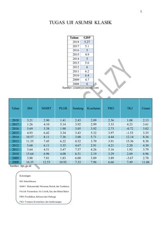
1. 1
TUGAS UJI ASUMSI KLASIK
Tahun GDP
2018 5.27
2017 5.1
2016 5
2015 4.9
2014 5
2013 5.6
2012 6
2011 6.2
2010 6.4
2009 4.7
2008 6
Sumber: countryeconomy.com
Tahun BM MMRT PLGB Sandang Kesehatan PRO TKJ Umum
2018 3.21 2.90 1.41 2.43 2.09 2.36 1.08 2.13
2017 1.26 4.10 5.14 3.92 2.99 3.33 4.23 3.61
2016 5.69 5.38 1.90 3.05 3.92 2.73 -0.72 3.02
2015 4.93 6.42 3.34 3.43 5.32 3.97 -1.53 3.35
2014 10.57 8.11 7.36 3.08 5.71 4.44 12.14 8.36
2013 11.35 7.45 6.22 0.52 3.70 3.91 15.36 8.38
2012 5.68 6.11 3.35 4.67 2.91 4.21 2.20 4.30
2011 3.64 4.51 3.47 7.57 4.26 5.16 1.92 3.79
2010 15.64 6.96 4.08 6.51 2.19 3.29 2.69 6.96
2009 3.88 7.81 1.83 6.00 3.89 3.89 -3.67 2.78
2008 16.35 12.53 10.92 7.33 7.96 6.66 7.49 11.06
Sumber: bps.go.id
Keterangan:
BM: BahanMakanan
MMRT: MakananJadi, Minuman,Rokok, dan Tembakau
PALGB: Perumahan, Air,Listrik, Gas, dan Bahan Bakar
PRO: Pendidikan, Rekreasi dan Olahraga
TKJ: Transpor,Komunikasi, dan JasaKeuangan

2. 2
A. Uji Normalitas
B. Uji Linieritas
Ramsey RESET Test:
F-statistic 0.046257 Probability 0.865134
Log likelihood ratio 0.497407 Probability 0.480642
Test Equation:
Dependent Variable: GDP
Method: Least Squares
Date: 10/29/18 Time: 11:37
Sample: 2008 2018
Included observations: 11
Variable Coefficient Std. Error t-Statistic Prob.
C 0.341663 19.77391 0.017278 0.9890
BM 0.373980 3.379309 0.110668 0.9298
MMRT 0.759823 6.495652 0.116974 0.9259
PLGB 0.633660 5.496272 0.115289 0.9269
SANDANG 0.269416 2.415164 0.111552 0.9293
KESEHATAN 0.413839 3.445293 0.120117 0.9239
PRO -0.829305 6.956820 -0.119208 0.9245
TKJ 0.496268 4.303225 0.115325 0.9269
UMUM -2.511216 21.89221 -0.114708 0.9273
FITTED^2 0.207551 0.965021 0.215074 0.8651
R-squared 0.980609 Mean dependent var 5.470000
Adjusted R-squared 0.806090 S.D. dependent var 0.592706
S.E. of regression 0.260999 Akaike info criterion -0.428310
Sum squared resid 0.068121 Schwarz criterion -0.066587
Log likelihood 12.35571 F-statistic 5.618913
Durbin-Watson stat 2.395550 Prob(F-statistic) 0.316979
0
1
2
3
4
-0.15 -0.10 -0.05 0.00 0.05 0.10 0.15 0.20
Series: Residuals
Sample20082018
Observations 11
Mean 6.20E-16
Median -0.021747
Maximum 0.166618
Minimum -0.136828
Std. Dev. 0.084423
Skewness 0.320659
Kurtosis 2.682129
Jarque-Bera 0.234818
Probability 0.889221

3. 3
C. Uji Autokorelasi
1. Durbin – Watson = 2,39
Ho : tidak ada serial autokorelasi baik positif maupun negatif
Sehingga tidak ada autokorelasi.
2. B-G test
Breusch-Godfrey Serial Correlation LM Test:
F-statistic 0.509274 Probability 0.605412
Obs*R-squared 3.711726 Probability 0.054031
Test Equation:
Dependent Variable: RESID
Method: Least Squares
Date: 10/29/18 Time: 11:44
Variable Coefficient Std. Error t-Statistic Prob.
C 0.035593 0.298186 0.119364 0.9244
BM -0.103063 0.647244 -0.159233 0.8995
MMRT -0.160062 0.525916 -0.304349 0.8119
PLGB -0.132090 0.791819 -0.166818 0.8948
SANDANG -0.131367 0.291761 -0.450255 0.7307
KESEHATAN -0.025990 0.119420 -0.217632 0.8636
PRO 0.116336 0.362141 0.321244 0.8021
TKJ -0.156087 0.521715 -0.299180 0.8149
UMUM 0.604472 2.931577 0.206193 0.8705
RESID(-1) -1.603578 2.247059 -0.713634 0.6054
R-squared 0.337430 Mean dependent var 5.92E-16
Adjusted R-squared -5.625704 S.D. dependent var 0.084423
S.E. of regression 0.217308 Akaike info criterion -0.794720
Sum squared resid 0.047223 Schwarz criterion -0.432997
Log likelihood 14.37096 F-statistic 0.056586
Durbin-Watson stat 1.760922 Prob(F-statistic) 0.997706

4. 4
Dari hasil uji autokorelasi, diketahui bahwa nilai probabilitas lebih besar dari
probabilitas 5%, maka hipotesa yang menyatakan pada model tidak terdapat autokorelasi
tidak ditolak. Berarti model empiric lolos dari masalah autokorelasi.
D. Homoskedastisitas
1. Uji White
Langkah-langkah pengujian White:
a. Lakukan estimasi model awaL:
GDP C BM MMRT PLGB SANDANG
Dependent Variable: GDP
Method: Least Squares
Date: 10/29/18 Time: 11:58
Sample: 2008 2018
Included observations: 11
Variable Coefficient Std. Error t-Statistic Prob.
C 5.187519 0.398402 13.02081 0.0000
BM 0.110234 0.040179 2.743553 0.0336
MMRT -0.232108 0.097044 -2.391772 0.0539
PLGB 0.064498 0.075011 0.859840 0.4229
SANDANG 0.157929 0.061978 2.548133 0.0436
R-squared 0.717078 Mean dependent var 5.470000
Adjusted R-squared 0.528463 S.D. dependent var 0.592706
S.E. of regression 0.407002 Akaike info criterion 1.342959
Sum squared resid 0.993905 Schwarz criterion 1.523821
Log likelihood -2.386276 F-statistic 3.801813
Durbin-Watson stat 1.315735 Prob(F-statistic) 0.071364
b. Dari tampilan equation:
White Heteroskedasticity Test:
F-statistic 0.320760 Probability 0.900251
Obs*R-squared 6.181864 Probability 0.626868
Test Equation:
Dependent Variable: RESID^2
Method: Least Squares
Date: 10/29/18 Time: 11:58
Sample: 2008 2018
Included observations: 11
Variable Coefficient Std. Error t-Statistic Prob.
C -0.020509 0.701552 -0.029233 0.9793
BM 0.146182 0.125509 1.164715 0.3643
BM^2 -0.008039 0.006720 -1.196291 0.3542
MMRT -0.437790 0.590292 -0.741649 0.5356
MMRT^2 0.036732 0.050913 0.721463 0.5456
PLGB 0.341466 0.398605 0.856652 0.4819
PLGB^2 -0.037162 0.047654 -0.779818 0.5171

5. 5
SANDANG 0.115245 0.145929 0.789734 0.5124
SANDANG^2 -0.012017 0.016188 -0.742356 0.5352
R-squared 0.561988 Mean dependent var 0.090355
Adjusted R-squared -1.190062 S.D. dependent var 0.126769
S.E. of regression 0.187603 Akaike info criterion -0.577359
Sum squared resid 0.070390 Schwarz criterion -0.251808
Log likelihood 12.17547 F-statistic 0.320760
Durbin-Watson stat 1.882165 Prob(F-statistic) 0.900251
c. Bandingkan nilai OBS*R2 dengan >> table dengan (df 9 dan =5% )=16,919. Tidak
significant
2. Uji LM ARCH
ARCH Test:
F-statistic 0.424084 Probability 0.533162
Obs*R-squared 0.503418 Probability 0.478002
Test Equation:
Dependent Variable: RESID^2
Method: Least Squares
Date: 10/29/18 Time: 12:13
Sample(adjusted): 2009 2018
Included observations: 10 after adjusting endpoints
Variable Coefficient Std. Error t-Statistic Prob.
C 0.076600 0.054603 1.402865 0.1983
RESID^2(-1) 0.224666 0.344995 0.651217 0.5332
R-squared 0.050342 Mean dependent var 0.098858
Adjusted R-squared -0.068365 S.D. dependent var 0.130277
S.E. of regression 0.134657 Akaike info criterion -0.995314
Sum squared resid 0.145060 Schwarz criterion -0.934797
Log likelihood 6.976571 F-statistic 0.424084
Durbin-Watson stat 2.005980 Prob(F-statistic) 0.533162
E. Uji Multikolinieritas
1. Pendekatan Korelasi Parsial
Dependent Variable: GDP
Method: Least Squares
Date: 10/29/18 Time: 11:08
Sample: 2008 2018
Included observations: 11
Variable Coefficient Std. Error t-Statistic Prob.
C 4.593835 0.255384 17.98792 0.0031
BM -0.334312 0.548084 -0.609964 0.6040
MMRT -0.631808 0.413231 -1.528946 0.2659
PLGB -0.531595 0.668795 -0.794856 0.5100
SANDANG -0.246721 0.196638 -1.254695 0.3363

6. 6
KESEHATAN -0.326570 0.098798 -3.305432 0.0806
PRO 0.664591 0.280914 2.365811 0.1417
TKJ -0.421120 0.411462 -1.023472 0.4137
UMUM 2.141076 2.438039 0.878196 0.4725
R-squared 0.979712 Mean dependent var 5.470000
Adjusted R-squared 0.898560 S.D. dependent var 0.592706
S.E. of regression 0.188775 Akaike info criterion -0.564910
Sum squared resid 0.071272 Schwarz criterion -0.239359
Log likelihood 12.10700 F-statistic 12.07255
Durbin-Watson stat 2.334466 Prob(F-statistic) 0.078716
Hasil estimasi persamaan awal dengan R2 = 0,98
2. Lakukan Regresi Antar Variable Bebas
(1) BM C MMRT PLGB SANDANG KESEHATAN PRO TKJ UMUM
Dependent Variable: BM
Method: Least Squares
Date: 10/29/18 Time: 11:16
Sample: 2008 2018
Included observations: 11
Variable Coefficient Std. Error t-Statistic Prob.
C 0.086351 0.264361 0.326639 0.7654
MMRT -0.737737 0.089799 -8.215410 0.0038
PLGB -1.212107 0.081208 -14.92595 0.0007
SANDANG -0.324995 0.087743 -3.703941 0.0342
KESEHATAN 0.025180 0.103053 0.244336 0.8227
PRO -0.391122 0.191241 -2.045172 0.1334
TKJ -0.745263 0.052201 -14.27689 0.0007
UMUM 4.442543 0.130535 34.03337 0.0001
R-squared 0.999556 Mean dependent var 7.472727
Adjusted R-squared 0.998521 S.D. dependent var 5.170691
S.E. of regression 0.198855 Akaike info criterion -0.237222
Sum squared resid 0.118630 Schwarz criterion 0.052156
Log likelihood 9.304723 F-statistic 965.4608
Durbin-Watson stat 3.377914 Prob(F-statistic) 0.000051
Diketahui bahwa R2
a mempunyai nilai sebesar 0,98 dan hasil estimasi persamaan
awal dengan R2 = 0,99. Maka, R2
a lebih rendah dibandingkan dengan nilai dari R2
pada regresi antar variable bebas BM,sehingga dalam model empirik dapat
dinyatakan terdapat adanya multikolinieritas.
(2) MMRT C BM PLGB SANDANG KESEHATAN PRO TKJ UMUM
Dependent Variable: MMRT
Method: Least Squares
Date: 10/29/18 Time: 11:20
Sample: 2008 2018
Included observations: 11
Variable Coefficient Std. Error t-Statistic Prob.

7. 7
C 0.126935 0.349206 0.363495 0.7403
BM -1.297809 0.157973 -8.215410 0.0038
PLGB -1.580411 0.201405 -7.846919 0.0043
SANDANG -0.441753 0.102131 -4.325348 0.0228
KESEHATAN 0.038842 0.136203 0.285177 0.7941
PRO -0.471037 0.282992 -1.664490 0.1946
TKJ -0.984322 0.086731 -11.34911 0.0015
UMUM 5.818593 0.563711 10.32194 0.0019
R-squared 0.996829 Mean dependent var 6.570909
Adjusted R-squared 0.989431 S.D. dependent var 2.565558
S.E. of regression 0.263749 Akaike info criterion 0.327623
Sum squared resid 0.208690 Schwarz criterion 0.617001
Log likelihood 6.198076 F-statistic 134.7429
Durbin-Watson stat 3.231004 Prob(F-statistic) 0.000965
Diketahui bahwa R2
a mempunyai nilai sebesar 0,98 dan hasil estimasi persamaan
awal dengan R2 = 0,996. Maka, R2
a lebih rendah dibandingkan dengan nilai dari R2
pada regresi antar variable bebas “MMRT”,sehingga dalam model empirik dapat
dinyatakan terdapat adanya multikolinieritas.
(3) PLGB C BM MMRT SANDANG KESEHATAN PRO TKJ UMUM
Dependent Variable: PLGB
Method: Least Squares
Date: 10/29/18 Time: 11:23
Sample: 2008 2018
Included observations: 11
Variable Coefficient Std. Error t-Statistic Prob.
C 0.052251 0.218392 0.239251 0.8263
BM -0.814048 0.054539 -14.92595 0.0007
MMRT -0.603351 0.076890 -7.846919 0.0043
SANDANG -0.262969 0.075926 -3.463505 0.0405
KESEHATAN 0.028381 0.083700 0.339082 0.7569
PRO -0.316554 0.159394 -1.985977 0.1412
TKJ -0.605406 0.063223 -9.575771 0.0024
UMUM 3.624879 0.223124 16.24601 0.0005
R-squared 0.999005 Mean dependent var 4.456364
Adjusted R-squared 0.996684 S.D. dependent var 2.829937
S.E. of regression 0.162963 Akaike info criterion -0.635319
Sum squared resid 0.079671 Schwarz criterion -0.345940
Log likelihood 11.49425 F-statistic 430.3708
Durbin-Watson stat 3.409060 Prob(F-statistic) 0.000170
Diketahui bahwa R2
a mempunyai nilai sebesar 0,98 dan hasil estimasi persamaan
awal dengan R2 = 0,99. Maka, R2
a lebih rendah dibandingkan dengan nilai dari R2
pada regresi antar variable bebas “PLGB”,sehingga dalam model empirik dapat
dinyatakan terdapat adanya multikolinieritas.

8. 8
(4) SANDANG C BM MMRT PLGB KESEHATAN PRO TKJ UMUM
Dependent Variable: SANDANG
Method: Least Squares
Date: 10/29/18 Time: 11:28
Sample: 2008 2018
Included observations: 11
Variable Coefficient Std. Error t-Statistic Prob.
C 0.198763 0.741003 0.268235 0.8059
BM -2.524857 0.681668 -3.703941 0.0342
MMRT -1.950880 0.451034 -4.325348 0.0228
PLGB -3.041976 0.878294 -3.463505 0.0405
KESEHATAN -0.054941 0.288342 -0.190540 0.8611
PRO -0.661305 0.731104 -0.904529 0.4324
TKJ -1.973756 0.401161 -4.920110 0.0161
UMUM 11.37559 2.847331 3.995176 0.0281
R-squared 0.981340 Mean dependent var 4.410000
Adjusted R-squared 0.937799 S.D. dependent var 2.222368
S.E. of regression 0.554263 Akaike info criterion 1.812908
Sum squared resid 0.921623 Schwarz criterion 2.102287
Log likelihood -1.970996 F-statistic 22.53830
Durbin-Watson stat 2.801899 Prob(F-statistic) 0.013464
Diketahui bahwa R2
a mempunyai nilai sebesar 0,98 dan hasil estimasi persamaan
awal dengan R2 = 0,981. Maka, R2
a lebih rendah dibandingkan dengan nilai dari R2
pada regresi antar variable bebas “Sandang”,sehingga dalam model empirik dapat
dinyatakan terdapat adanya multikolinieritas.
(5) KESEHATAN C BM MMRT PLGB SANDANG PRO TKJ UMUM
Dependent Variable: KESEHATAN
Method: Least Squares
Date: 10/29/18 Time: 12:16
Sample: 2008 2018
Included observations: 11
Variable Coefficient Std. Error t-Statistic Prob.
C -0.153797 1.489757 -0.103236 0.9243
BM 0.774902 3.171463 0.244336 0.8227
MMRT 0.679502 2.382735 0.285177 0.7941
PLGB 1.300535 3.835458 0.339082 0.7569
SANDANG -0.217637 1.142211 -0.190540 0.8611
PRO 1.456416 1.409885 1.033003 0.3776
TKJ 0.369327 2.395006 0.154207 0.8872
UMUM -3.439492 14.10821 -0.243794 0.8231
R-squared 0.876562 Mean dependent var 4.085455
Adjusted R-squared 0.588541 S.D. dependent var 1.719775
S.E. of regression 1.103151 Akaike info criterion 3.189481
Sum squared resid 3.650826 Schwarz criterion 3.478859
Log likelihood -9.542144 F-statistic 3.043395
Durbin-Watson stat 2.529631 Prob(F-statistic) 0.194813

9. 9
Diketahui bahwa R2
a mempunyai nilai sebesar 0,98 dan hasil estimasi persamaan
awal dengan R2 = 0,876. Maka, R2
a lebih tinggi dibandingkan dengan nilai dari R2
pada regresi antar variable bebas “Kesehatan”,sehingga dalam model empirik tidak
terdapat adanya multikolinieritas.
(6) PRO C BM MMRT PLGB SANDANG KESEHATAN TKJ UMUM
Dependent Variable: PRO
Method: Least Squares
Date: 11/19/18 Time: 10:55
Sample: 2008 2018
Included observations: 11
Variable Coefficient Std. Error t-Statistic Prob.
C 0.366539 0.480328 0.763101 0.5009
BM -1.488875 0.727995 -2.045172 0.1334
MMRT -1.019277 0.612366 -1.664490 0.1946
PLGB -1.794257 0.903464 -1.985977 0.1412
SANDANG -0.324032 0.358233 -0.904529 0.4324
KESEHATAN 0.180150 0.174394 1.033003 0.3776
TKJ -1.034973 0.598400 -1.729568 0.1821
UMUM 6.480513 3.333011 1.944342 0.1471
R-squared 0.967594 Mean dependent var 3.995455
Adjusted R-squared 0.891980 S.D. dependent var 1.180478
S.E. of regression 0.387980 Akaike info criterion 1.099535
Sum squared resid 0.451585 Schwarz criterion 1.388913
Log likelihood 1.952558 F-statistic 12.79654
Durbin-Watson stat 3.510158 Prob(F-statistic) 0.030177
Diketahui bahwa R2
a mempunyai nilai sebesar 0,98 dan hasil estimasi persamaan
awal dengan R2 = 0,967. Maka, R2
a lebih tinggi dibandingkan dengan nilai dari R2
pada regresi antar variable bebas “PRO”,sehingga dalam model empirik tidak
terdapat adanya multikolinieritas.
(7) TKJ C BM MMRT PLGB SANDANG KESEHATAN PRO UMUM
Dependent Variable: TKJ
Method: Least Squares
Date: 11/19/18 Time: 10:57
Sample: 2008 2018
Included observations: 11
Variable Coefficient Std. Error t-Statistic Prob.
C 0.120479 0.351531 0.342727 0.7544
BM -1.322345 0.092621 -14.27689 0.0007
MMRT -0.992803 0.087479 -11.34911 0.0015
PLGB -1.599456 0.167032 -9.575771 0.0024
SANDANG -0.450783 0.091621 -4.920110 0.0161
KESEHATAN 0.021294 0.138084 0.154207 0.8872
PRO -0.482411 0.278920 -1.729568 0.1821
UMUM 5.902999 0.296561 19.90485 0.0003

10. 10
R-squared 0.999374 Mean dependent var 3.744545
Adjusted R-squared 0.997914 S.D. dependent var 5.799323
S.E. of regression 0.264882 Akaike info criterion 0.336202
Sum squared resid 0.210488 Schwarz criterion 0.625580
Log likelihood 6.150891 F-statistic 684.3498
Durbin-Watson stat 3.310285 Prob(F-statistic) 0.000085
Diketahui bahwa R2
a mempunyai nilai sebesar 0,98 dan hasil estimasi persamaan
awal dengan R2 = 0,99. Maka, R2
a lebih rendah dibandingkan dengan nilai dari R2
pada regresi antar variable bebas “TKJ”,sehingga dalam model empirik dapat
dinyatakan terdapat adanya multikolinieritas.
(8) UMUM C BM MMRT PLGB SANDANG KESEHATAN PRO TKJ
Dependent Variable: UMUM
Method: Least Squares
Date: 11/19/18 Time: 10:58
Sample: 2008 2018
Included observations: 11
Variable Coefficient Std. Error t-Statistic Prob.
C -0.019171 0.059456 -0.322434 0.7683
BM 0.224515 0.006597 34.03337 0.0001
MMRT 0.167156 0.016194 10.32194 0.0019
PLGB 0.272771 0.016790 16.24601 0.0005
SANDANG 0.073999 0.018522 3.995176 0.0281
KESEHATAN -0.005648 0.023168 -0.243794 0.8231
PRO 0.086035 0.044249 1.944342 0.1471
TKJ 0.168132 0.008447 19.90485 0.0003
R-squared 0.999931 Mean dependent var 5.249091
Adjusted R-squared 0.999768 S.D. dependent var 2.937535
S.E. of regression 0.044704 Akaike info criterion -3.222263
Sum squared resid 0.005995 Schwarz criterion -2.932885
Log likelihood 25.72245 F-statistic 6168.119
Durbin-Watson stat 3.373122 Prob(F-statistic) 0.000003
Diketahui bahwa R2
a mempunyai nilai sebesar 0,98 dan hasil estimasi persamaan
awal dengan R2 = 0,99. Maka, R2
a lebih rendah dibandingkan dengan nilai dari R2
pada regresi antar variable bebas “UMUM”,sehingga dalam model empirik dapat
dinyatakan terdapat adanya multikolinieritas.