Manual de programación CNC simulator 2.0

1. SOFTWARE CNC LATHE MACHINE SIMULATOR
© VirtLabs Software (https://virtlabs.tech/cnc-simulator/)
INTRODUCTION
The methodology for the development of simulation models and simulators in various
technical disciplines is mainly focused on reducing the level of abstraction of educational
material. Along with theoretical educational material, visual simulation of a particular
technological process or operation allows the student to more fully master the taught material
with the maximum approximation to natural conditions. At the same time, simulation models and
simulators can only be considered as an auxiliary tool of the educational process. The main
purpose of this category of educational resources is basic (initial) introduction to the principles
of operation of complex technical objects in the absence of the possibility of using real industrial
equipment, or for the purpose of preliminary improvement of the student's competence before
passing industrial practice.
Of particular relevance is the methodology of combining educational tasks with
engineering and applied tasks in a single toolkit that meets the current level of development of
technology and industry as a whole. Here we are talking about the integrated implementation of
computer-aided design (CAD/CAM) functions and the principles of simulation-numerical
simulation of technological processes.
The main tendency to introduce simulation training models in engineering education is to
achieve maximum interactivity. A prerequisite here is the ability to perform «erroneous» actions
by students and an adequate response of the simulation model to these actions in order to achieve
the required level of understanding of educational material for students. The higher the degree of
freedom of the simulated object (device or machine), the greater the effect of real interaction is
achieved in the learning process.
Keywords: simulator, model, training, verification, software, system, control, CNC,
turning, machine, processing, technology, design, program, cycle, code, shaping, standard.
PURPOSE AND OBJECTIVES OF THE PROJECT
The purpose of the presented project is to develop an educational and methodological
software product (simulation model or simulator) intended for basic familiarization of novice
machine-building specialists with the principles of programming operations of turning parts
using standard G/M-code.
Fields of application of the software product primarily cover the educational process
using computer technology in the form of laboratory classes for students in computer classes,
distance learning, as well as demonstration support of lecture material in the group of training
areas and specialties «Metallurgy, Mechanical Engineering and Material Processing». The
flexible functionality and mobility of the software product also allows it to be used as an
application tool for verification and preliminary testing of control programs for material turning
operations on numerically controlled machines (CNC) using Fanuc program code (code system
A).
The functionality of the simulator should provide the following tasks:
 preparation of texts of control programs for turning operations in the format of a
standard G/M code and verification of control programs for syntactic and technological errors;

2.  reproduction on the screen of a computing device of three-dimensional graphic models
of the main units of the simulated equipment, technological equipment and metal-cutting tools
for the purpose of educational simulation of the turning process of the material;
 three-dimensional visualization of the process of workpiece forming during turning
according to compiled control programs;
 visualization of the movement paths of the cutting tool in the working plane of the
machine;
 user interaction with a simulation equipment model.
The technical advantage of the developed simulator is a relatively low resource intensity
and multi-platform support, which allows using this software on various computing devices,
including interactive whiteboards, smartphones, tablets and desktop computers, which, in turn,
increases the flexibility and mobility of the educational process, corresponding to the modern
level of Informatization of education.
MODELING OBJECT
The basis of the three-dimensional simulation model is the TC1625 lathe machine
manufactured by the Tver machine-tool plant «StankoMachComplex» with a horizontal bed and
a classic assembly of units, equipped with a CNC system, an eight-position turret, a three-jaw
turning chuck, a tailstock, a lubricant-coolant supply system and other units. Material processing
is performed in two coordinates in the horizontal plane of the machine. The main technical
characteristics of the prototype equipment are presented in table 1.
Table 1 – Basic Specifications of a TC1625 Lathe Machine
№ Characteristic Value
1 Overall dimensions LxWxH, mm 2775х1585х1670
2 Distance between centers, mm 1000
3 Spindle bore diameter, mm 77
4 Diameter of 3-jaw chuck, mm 250
5 Width of guides, mm 440
6 X/Z axis positioning accuracy, mm ±0.005
7 Quick movements along the X/Z axes, mm/min 8000/12000
8 Working feed, mm/min 0.01~6000
9 Spindle speed range, rpm 10–1650
10 Number of tools 8
11 Tool change time, s 0.8
The software simulates a set of cutting tools (turning tools and drills), including 185
items. The types of replaceable cutting inserts used for turning tools are presented in table 2.

3. Table 2 – Types of Interchangeable Cutting Plates Used Turning Tools
Letter
Designation
According to
ISO13399
Plate Geometric Shape
Name of the Plate
Geometric Shape
Main Angle
in the Plan
S Square 90
T Triangular 60
C
Rhombic
80
D 55
E 75
F 50
M 86
V 35
W Trigonal 80
R Round -
Also in the model, cutters with special thread-cutting plates and drills are used. Figure 1
shows a geometric model of a turning tool.
Figure 1 – Geometrical Model of a Turning Tool and Designation of the Main Characteristics of
an Interchangeable Cutting Plate: Main Angle in the Plan (φ1), Auxiliary Angle in the Plan (φ2),
Diameter of the Inscribed Circle (D), Radius of Rounding at the Vertex ®

4. GEOMETRIC MODELING METHODOLOGY
In the simulator, a simplified model of shaping the workpiece is used, based on the
assumption that the axial symmetry of the part is constant throughout the entire turning process
[1, 2]. This model excludes the possibility of constructing screw surfaces, and threaded elements
of parts are depicted conditionally - by sections of concentric ribbing. Basic calculations using
this technique are formalized by the geometric problem of intersecting two flat closed loops in
the working plane of the machine — the contour of the workpiece and the contour of the cutting
tool. Based on the shape-forming contour, which is a logical difference at the intersection of the
two source loops, a three-dimensional surface of the simulated part is formed by uniformly
turning the shape-forming contour around the main axis of the machine (axis of rotation of the
workpiece). The applied method makes it possible to simulate the shaping of a part such as a
body of revolution in real time at relatively low computational costs.
The initial stage of the algorithm is the formation of many points Wi of the contour of the
workpiece (Fig. 2.a). In the initial state (before the start of the processing process), the part
contour includes four points, while the longitudinal section of the part is represented by a
rectangle. In subsequent iterations of the algorithm, the initial contour of the part is the
previously calculated shape-forming contour. The contour is described counterclockwise.
At the second stage of the algorithm, the contour of the turning insert of the turning tool
is formed taking into account its geometric characteristics – overall dimensions, the main angle
in plan and the radius of rounding at the apex. The contour of the insert is described by points Cj
in the opposite direction with respect to the contour of the part (clockwise).
Figure 2 – To the Task of Calculating the Shaping Contour of the Workpiece:
Intersection of the Original Contours of the Workpiece and the Cutting Plate (a); Obtaining the
Shape-Forming Contour of the Workpiece as the Logical Difference of the Original Contours (b)
The third stage of the algorithm is to determine the set of intersection points Ik of the
original contours. Moreover, the found intersection points are indexed in accordance with how
much closer they lie to the starting point of the part’s contour, and are included in the
generalized set of points of both contours in the indexing order. The coordinates of the
intersection points are determined for two segments belonging to two different contours (Fig. 3).
С1
С2
С3
С4 С5
С6
W1
W2 W3
W4 W5
W6
I1
I2
F5
F6
F7 F8
F1
F2 F3
F10 F11
F12
F4
F9
a b

5. Figure 3 – To the Determination of the Coordinates of the Intersection Point of Two Segments
For the segments P1–P2 and P3–P4 belonging to two intersecting straight lines L1 and L2,
it follows:

























4
3
2
4
3
2
2
1
1
1
2
1
2
2
2
2
1
1
1
1
,
,
,
,
,
x
x
B
y
y
A
x
x
B
y
y
A
C
y
B
x
A
L
C
y
B
x
A
L
(1)
The x, y coordinates of the intersection point of the lines L1 and L2 are determined by the
matrix equation:



















2
1
2
2
1
1
C
C
y
x
B
A
B
A
(2)
hence:










































2
1
1
2
1
2
1
2
2
1
2
1
1
2
2
1
1
1
C
C
A
A
B
B
B
A
B
A
y
x
C
C
B
A
B
A
y
x
(3)
The points of the generalized set belonging to the contour of the cutting insert, outside the
intervals between the points of intersection, are excluded from the generalized set of points of
both contours. Thus, the final set of points Fn is formed that describe the shape-forming contour
of the part (Fig. 2.b). The resulting contour is described in the same direction as the original
contour of the workpiece.
The considered algorithm is a simplified version of the Weiler–Atherton cut-off
algorithm [3]. A number of simplifications of the algorithm is due to the geometric features of
the problem being solved, namely: a constant condition for the convexity of the cutting insert
contour, conditions for detecting collisions of inoperative elements of the cutter (holder) with the
workpiece, the condition for excluding the completely cut-off part of the part from the
computational process when modeling the operation segments, etc.
L1 L2
P1(x1,y1)
P4(x4,y4)
P2(x2,y2)
P3(x3,y3)

6. Due to the fact that the shaping of the part is carried out during the movement of the
cutting tool, at each iteration of the algorithm, a discrete change in the coordinates of the points
of the contour of the cutting insert relative to the contour of the workpiece occurs. The step of
discreteness in this case is due to a given parameter of the movement of the cutting tool (the
value of the working feed) and the iteration time of the simulation cycle. In this case, the step of
discreteness of movement of the tool (δ) can exceed the linear dimensions of the overlapping
area of the contours of the cutting insert and the workpiece (Fig. 4.a), which leads to the
appearance of artifacts («uncut» sections) of the forming contour of the part (Fig. 4.b )
Figure 4 – The Problem of Discreteness of Calculating Contour Intersections
One solution to the described problem is the Jarvis method, which consists in
constructing a minimal convex hull around the set of vertices of the contours of the cutting insert
in the current and previous discrete states (Fig. 5).
Figure 5 – Construction of a Minimal Convex Hull Around the Contours of the Cutting Plate in
Two Successive Discrete States
In this case, the intersection of the contour of the workpiece with the contour of the
minimum convex shell is calculated, which provides the required overlap area in the gaps
between the discrete states of the cutting tool. When constructing a minimal convex hull, the
condition of invariance of the circumvention of its contour is especially important. The minimum
convex hull can cover several discrete states of the cutting insert, provided that the direction of
Feed Direct
δ
a b
Shape Contour Artifact
Contour of the Cutting
Plate in the Discrete State i
Contour of the Cutting
Plate in the Discrete State
i–1
Minimal Convex
Hull

7. the working feed of the tool does not change in these conditions (the tool moves along a straight
path).
In the project under consideration, an alternative method of eliminating artifacts of the
formative contour is used, based on the Ramer-Douglas-Peker generalization algorithm [4, 5],
which is widely used in topography and cartography problems. The main goal of the recursive
generalization procedure is to reduce the number of vertices of the polyline based on a given
threshold value of the distance between the vertices. The initial condition for the algorithm to
work is to select the most distant point with respect to the starting point of the polyline of the
contour. In subsequent iterations of the algorithm, the distances between the intermediate points
of the polyline are determined and compared with the threshold value. The connection of points
in the approximating polyline is carried out provided that the distance between them exceeds a
predetermined threshold value (Fig. 6).
Figure 6 – Iterations of the Ramer-Douglas-Pecker Generalization Algorithm as an Example of
an Arbitrary Polyline
Technically, the procedure for approximating the shape-forming contour of a part is
combined with the initial stage of the general modeling algorithm, at which many vertices of the
initial contour of the workpiece are formed.
The formation of a three-dimensional surface of the simulated part is carried out by
calculating the coordinates of the points in the circles of the cross sections of the part along the
length of the shape-forming contour, followed by combining these points into triangular facets
(between sections). The length of the radius vector Ri of each point of the forming contour is
calculated as the distance from this point to the main axis of the machine (Fig. 7).
Iteration 1 Iteration 2
Iteration 3 Iteration 4
Original
Polyline
Current
Approximation
Previous
Approximation
(Finish)

8. Figure 7 – Polygon Model of a Rotation Body Workpiece in a Section
(splitting polygons into triangular facets is not shown)
The order of traversal of the vertices when assembling a three-dimensional frame is
strictly defined. Each polygon of a three-dimensional surface is divided into 2 triangular facets,
uniting 4 vertices (Fig. 8). The radial smoothness of the formed three-dimensional surface
depends on a given number of segments (circle sectors) in the section of the simulated part. The
procedure for assembling a three-dimensional framework also calculates the normal vectors at
each vertex (Fig. 9) and the texture coordinates of UV. According to the calculated texture
coordinates, the surface of the part is drawn with an overlaid image of the metal texture, which in
turn increases the realism of perception of the simulated process.
Thus, the final three-dimensional model of the workpiece allows you to visualize the
results of material removal by the cutter in real-time dynamics with the required degree of
realism.
Shaping
Contour
Main Axis
of the Machine
Design Cross-Sections
of the Workpiece
Ri

9. Рисунок 8 – Faceted Frame of a Three-Dimensional Model of the Workpiece, Inscribed in the
Overall Cylinder of the Original Workpiece
Figure 9 – Normal Vectors at the Vertices of the Faceted Model of the Workpiece

10. PRINCIPLES OF NUMERICAL PROGRAM CONTROL SIMULATION
List of the Main Functions of the Machine Control
As a linguistic basis for programming the basic technological operations during material
turning, G-M codes of Fanuc numerical control system were released:
G00/G01 – linear interpolation at accelerated/working feed;
G02/G03 – circular interpolation clockwise / counterclockwise;
G04 – time delay;
G20/G21 – data entry in inches/millimeters;
G28 – return to the reference point;
G32/G34 – threading with constant/variable pitch in single-pass;
G40–G42 – automatic tool radius compensation;
G50 – setting the maximum spindle speed;
G53–G59 – switching between working coordinate systems №1–6;
G70–G76 – main turning cycles;
G80–G83 – drilling cycles;
G90 – the cycle of the main turning of the external/internal diameter;
G92 – constant-pitch threading cycle;
G94 – cycle of the main external/internal end turning;
G96/G97 – constant cutting/spindle speed;
G98/G99 – feed rate [mm/min]/ feed rate [mm/rev];
M00/M01 – software stop with confirmation;
M02/M30 – completion of the control program;
M03/M04 – start spindle rotation clockwise/counterclockwise;
M05 – spindle rotation stop;
M07–M09 – turning on/off the coolant supply;
M38/M39 – opening/closing of automatic doors;
M97–M99 – call and end of internal/external routines.
Structure and Format of the Control Program Code
The control program code is represented as a sequence of lines (frames). The simulator
allows you to develop and execute control programs up to 999 frames (taking into account the
first uneditable line containing the number of the control program). Each frame consists of a
sequence of words, which is a combination of an alphabetic address and a numerical parameter.
No spaces are allowed between the address and the parameter. The typing of the control program
is carried out in alphanumeric characters using a monospace font. Some special characters are
allowed. Any group of characters that cannot be parsed should be enclosed in parentheses or
written after the characters «;» or «/». This information is considered a comment on the code and
is not analyzed during the simulation. The addresses of the preparatory (G) and auxiliary (M)
functions are programmed with integer parameters defining the numbers of these functions.
Numerical positioning parameters (after addresses X, Z, U, W, I, K, R, etc.) can be specified in
fractional or integer values. The «minus» sign is allowed here.
After starting the simulation process, the control program code is automatically checked
for compliance with the format. In case of errors, the corresponding messages are displayed.

11. Brief Description of Control Program Parsing Algorithm
Syntactic analysis (parsing) of the control program code and simulation of its execution
are carried out according to the standard algorithm [6], the block diagram of which is shown in
Figure 10.
Figure 10 – Control Program Parsing Algorithm Flowchart
In accordance with the block diagram shown in Figure 10, parsing of the control program
begins with the formation of a list of frames. For each frame, a list of words is generated. A word
is a data structure — a command that includes a letter address and a numeric parameter. Teams
are conditionally classified as modal and positional.
Modal commands change the status of the simulation model of the machine, and
determine its current state – the mode of movement of the tool (moving at accelerated or
working feed, type of interpolation), spindle rotation mode, position of automatic doors,
condition of the cooling system, etc. In turn, positional commands directly determine the
parameters of movements – the coordinates of the end points, the parameters of the arcs during
circular interpolation, etc.
According to the obtained motion parameters, the coordinates of the cutting tool, the
rotation angles of the rotating elements of the machine, the position of the automatic doors, etc.
Creating a List of
Program Frames
Creating a Word List
Frame Reading
Word Reading
Creating a Command
(address and
parameter pair)
End of Frame
No
Yes
Motion
Simulation
Command
Getting Parameter
Value
Modal
Positional
Getting Parameter
Value
Model Status
Update
Saving the Current
Status of the Model
Movement Type
Determination
Motion Interpolation
Program End End
Yes
No

12. are interpolated. Thus, a frame-by-frame simulation of the control program occurs. When the last
frame is reached, the simulation process ends.
Implementation of Turning Tool Movement Control
By analogy with a real CNC system, the movement of the cutting tool is programmed by
linear and circular interpolation methods. Linear interpolation is the main type of movement
when machining on a CNC lathe. With linear interpolation, the tool moves along a straight path
with the known coordinates of its beginning and end (Fig. 11).
Figure 11 – Tool Path for Linear Interpolation
When the calculated point C moves from point A to point B along a rectilinear section
with a constant feed rate, both coordinates are linearly interpolated in time. Denoting the start
time of the movement as tA, and the end time as tB, the current coordinates of point C
corresponding to the current time tC can be determined by linear interpolation formulas:
 
A
B
A
C
B
A
A
C
t
t
t
t
Z
Z
Z
Z





 , (4)
 
A
B
A
C
B
A
A
C
t
t
t
t
X
X
X
X





 (5)
The final travel time is defined as:
S
A
B t
t
t 
 , (6)
where tS – time spent on straightforward movement at a constant feed rate F (mm/min):
   
F
X
X
Z
Z
t A
B
A
B
S
2
2



 (7)
Linear interpolation at rapid feed is programmed with the modal function G00 (this
function is active in the initial state of the CNC system). Linear interpolation at the feed rate is
programmed with the modal function G01. After these functions, the coordinates of the end point
of the straight section of the path are set. The current position of the tool is always taken as the
starting point. The set feedrate for rapid traverse is ignored. The coordinates of the end point can
be specified in absolute values (X, Z), that is, relative to zero of the working coordinate system,
or in relative (incremental) values (U, W), that is, relative to the starting point of a rectilinear
trajectory. If one of the coordinates is omitted, movement along its axis is not carried out.
Circular interpolation is used to grind curved surfaces, the shape of which is described by
an arc of a circle of a certain radius. Two arc programming methods are used. The first method is
X
0 Z
A
B
ZA
XA
XB
ZB
C
ZC
XC

13. to specify the coordinates of the center of the arc and the end point, while the radius of the arc is
calculated automatically. The second method involves specifying the radius of the arc and the
coordinates of the end point, while the coordinates of the center of the arc are automatically
calculated. Clockwise circular interpolation is set using function G02, and counterclockwise
circular interpolation is set by function G03, respectively.
Let us consider one of the cases of circular interpolation counterclockwise indicating the
center of the arc (Fig. 12.a). When the calculated point C moves from point A to point B along an
arc with a constant feed rate, both coordinates can also be interpolated in time. The trajectory of
motion is determined by the position of the end point B and the position of the center of the arc
O in incremental coordinates (i, k) relative to the starting point A.
The angular position of the radius vectors OA, OB and OC is described by the
trigonometric angles φA, φB and φC, respectively.
Figure 12 –Tool Path During Circular Interpolation Counterclockwise with the Programming of
the: Center of the Arc (a); Arc Radius (b)
Denoting the start time of the movement as tA, and the end time as tB, the angle φC
corresponding to the current time tC can be determined by the linear interpolation formula:
 
A
B
A
C
B
A
A
C
t
t
t
t





 


 , (8)
where φA, φB – trigonometric angles of radius vectors of the starting and ending points of the arc:








i
k
A arctan
2
3
 , (9)














B
A
B
A
B
Z
k
Z
X
i
X
arctan

 (10)
O–
X
0 Z
A
B
ZA
XB
XA
ZB
C
ZC
XC
O
k
i
φA
φB
φC
ZO
XO
r
a b
X
0
Z
A
B
ZA
XB
XA
ZB
r–
O+
r+

14. Note: when calculating the trigonometric angles of the extreme points of the arc, it is
necessary to take into account situations in which the arc tangent function takes singular values.
The Cartesian coordinates of point C are defined as:
 
C
A r
X 
sin

 , (11)
 
C
A r
Z 
cos

 , (12)
where
2
2
k
i
r 
 (13)
The final travel time is determined by the expression (6). In this case, the time tS spent on
moving along the arc at a constant feed rate F (mm/min) can be determined using the expression
for the length of the arc:
 
F
R
t A
B
S





180



(14)
The incremental coordinates of the center of the arc are programmed with addresses I and
K in the directions of the X and Z axes, respectively. When programming circular interpolation
with the center of the arc, it is necessary that the radius vectors of the start and end points of the
arc have the same length.
Circular interpolation is always performed on the working feedrate.
The second method of programming an arc is to indicate the radius of the arc circle. In
this case, two cases of setting the radius are allowed – with a positive or negative value. If the
radius value is positive, the arc angle is less than 180 degrees. Otherwise, the angle of the arc is
more than 180 degrees (Fig. 12.b). When defining an arc with a radius, the CNC system
automatically determines the position of the center of the arc (O+
or O–
depending on the sign of
the radius). In this method of defining an arc, the condition must be met: the radius modulus
cannot be less than half the length of the chord (AB) of the arc.
Figure 13 shows an example of the formation of a curved surface when programming
circular interpolation counterclockwise.
Figure 13 – Curved Surface Formation when Programming Circular Interpolation
Counterclockwise

15. Implementation of Coordinate Systems Functions
The presented simulation model includes several coordinate systems (Fig. 14). The main
and invariable coordinate system is the machine coordinate system with the origin corresponding
to the machine zero point M geometrically coinciding with the intersection point of the end plane
of the spindle and its axis of rotation.
Figure 14 – Basic Coordinate Systems of the Simulation Model
The second important coordinate system is the reference coordinate system with the
origin corresponding to the reference point R or tool change point. In this coordinate system, the
basic movements of the moving parts of the machine are calculated, and collisions of the tool
with the structural elements of the machine are determined when modeling possible emergency
situations.
The programming of the turning process is carried out in the working coordinate system.
The simulator provides 6 independent working coordinate systems with zero points W1–6. The
initial settings for the position of these zeros are set by the user in the parameters of the
simulation model and are designated as zero corrections.
The directions of the axes in each coordinate system are the same. The longitudinal axis
Z is always directed from the turning chuck towards the tailstock of the machine. The transverse
axis X (or the axis of the diameters) is directed towards the caliper (towards yourself with a front
view to the machine). The Y axis is the normal to the work plane ZX and is directed vertically
upward. Movements in the direction of the Y axis in the considered model of the machine are not
carried out.
Switching between working coordinate systems is carried out programmatically using the
corresponding functions G54–G59 (for coordinate systems with zero points W1–W6,
respectively). The zero coordinates W1–6 are calculated in the machine coordinate system relative
to machine zero M. The syntax of the functions G54–G59 suggests two possible ways to use
them. In the first version, the functions are set without specifying the X and Z coordinates. In
this case, the position of the selected working coordinate system is determined by the predefined
zero corrections. In this case, the functions G54–G59 can be programmed separately in an
individual block or in one block with other commands. The second option of using the G54–G59
functions involves the programmed displacement of the axes of the selected working coordinate
system relative to a predefined zero W1. In this case, the X and Z axis offsets are programmed
ZR
M
W
R
YR
XR
XW
ZW
YW
YM
XM
ZM

16. immediately after the function in the same block (for example, «G54 X30.5 Z15»). Figure 15
shows the position of the first coordinate origin after programmatically shifting the axes to a
point [X=10, Z=–20] relative to the initial zero position W1, specified in the zero corrector
settings block.
Figure 15 – Illustration of the Programmed Displacement of the Axes of the Working
Coordinate System №1
Programming with respect to machine zero is carried out via function G53. This function
is not modal, and is executed in the block in which it is programmed. The function temporarily
cancels the modal functions of the G54–G59. In this case, all movements are counted in the
coordinate system of the machine with the beginning at point M, and the active zero corrector is
temporarily canceled. The G53 function must be programmed whenever it is necessary to specify
the coordinates relating to machine zero. The syntax of the function does not imply the presence
of parameters after the word G53. The function is programmed in any block that has path control
commands (for example, «G53 G00 X0 Z120»). Figure 16 shows the position of the origin of the
working coordinate system during the operation of function G53.
Figure 16 – Illustration of the Position of the Origin of the Working Coordinate System During
the Operation of Function G53
–
–2
20
0
1
10
0

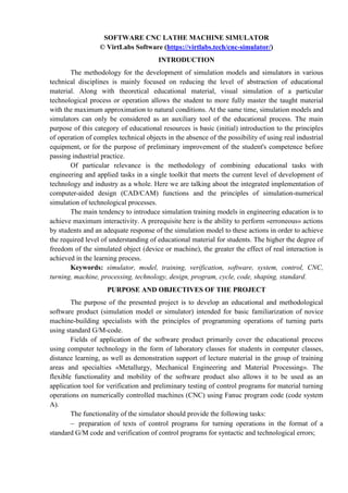
17. Implementation of Basic Turning and Drilling Cycles
The implemented control program parsing algorithm allows simulating the execution of
turning and drilling cycles of the Fanuc system. When each cycle is performed, a so-called buffer
list of frames is created in the memory of the computing device, including intermediate tool
movements when a programmed part contour is received. Turning cycles are defined by one or
two consecutive initiating frames, in which the main parameters of the cycle are prescribed -
roughing and finishing allowances, cutting depth during roughing with the cutter, number of
roughing with the cutting, amount of cutting back, parameters of the cutting mode, etc. The part
contour is programmed by a sequence of frames with the required numbering of the first and last
block.
The stock removal cycle parallel to the Z axis is initiated by function G71. The loop
parameters are programmed in two consecutive blocks in the format:
G71 U_ R_
G71 P_ Q_ U_ W_ F_ S_
where [first frame]: U – the depth of cut for the roughing passes (programming mode in the
radius), R – distance of retract after the end of each pass; [second frame]: P – number of the first
frame of the contour sequence; Q – number of the last frame of the contour sequence, U – the
value (programming mode in diameters) and the direction of removal of the finishing allowance
on the X-axis, W – the value and the direction of removal of the finishing allowance on the Z-
axis; F – feed rate for roughing; S – spindle speed/cutting speed during finishing.
Figure 17 shows the tool paths during the G71 turning cycle. The green lines show the
movements of the cutter in the working feed, the purple lines show the accelerated feed. As can
be seen from the figure, the processed circuit may include curved sections programmed by the
method of circular interpolation.
Figure 17 – Cutting Tool Path During the Execution of the Turning Cycle G71 and Control
Program Code Fragment
The stock removal cycle parallel to the X axis is triggered by function G72. The
programming principle of this cycle is similar to the G71 cycle. The execution of rough passes
by the cutter is carried out in the direction of the X axis of the working coordinate system. The
loop parameters are programmed in two consecutive blocks in the format:
G72 W_ R_
G72 P_ Q_ U_ W_ F_ S_
where [first frame]: W – the depth of cut for the roughing passes, R – distance of retract after the
end of each pass; [second frame]: P – number of the first frame of the contour sequence, Q –
G71 U4 R1;
G71 P10 Q20 U2 W1 F0.5;
N10 G00 X40;
G01 Z0;
Z-20;
X54;
U6 W-4;
Z-50;
G03 X80 Z-60 R10;
G01 X100;
N20 X102;

18. number of the last frame of the contour sequence, U – the value (programming mode in
diameters) and the direction of removal of the finishing allowance on the X-axis, W – the value
and the direction of removal of the finishing allowance on the Z-axis, F – feed rate for roughing,
S – spindle speed/cutting speed during finishing.
Figure 18 shows the tool paths during the G72 turning cycle.
Figure 18 – Cutting Tool Path During the Execution of the Turning Cycle G72 and Control
Program Code Fragment
The stock removal cycle parallel to the specified contour is initiated by function G73. The
loop parameters are programmed in two consecutive blocks in the format:
G73 U_ W_ R_
G73 P_ Q_ U_ W_ F_ S_
where [first frame]: U – the value (programming mode in the radius) and the direction of
removal of the total allowance on the X-axis, W – the value and the direction of removal of the
total allowance on the Z-axis, R – the number of consecutive passes when removing the rough
allowance, including a half-pass; [second frame]: P – number of the first frame of the contour
sequence; Q – number of the last frame of the contour sequence; U – the value (programming
mode in diameters) and the direction of removal of the finishing allowance on the X-axis, W –
the value and the direction of removal of the finishing allowance on the Z-axis, F – feed rate for
roughing, S – spindle speed/cutting speed during finishing.
Figure 19 shows the tool paths during the G73 turning cycle.
Figure 19 – Cutting Tool Path During the Execution of the Turning Cycle G73 and Control
Program Code Fragment
G72 W4 R1;
G72 P20 Q30 U1 W0.1 F0.8;
N20 G01 X0;
G01 W-2;
G02 U20 W-10 I0 K-10;
G01 Z-40;
N30 G01 X80;
G73 U4 W4 R3;
G73 P70 Q80 U1 W0.1 F0.9;
N70 G00 U-60 W-3 F0.35;
G01 G42 W-2;
G01 W-7;
G01 U6 W-8;
G01 W-5;
G01 U16 Z-32;
G03 X52 Z-37 R5;
G01 Z-50;
N80 G01 X80;

19. The finishing cycle is triggered by function G70. The loop parameters are programmed in
one block in the format:
G70 P_ Q_ F_ S_
where P – number of the first frame of the contour sequence, Q – number of the last frame of the
contour sequence, F – feed rate for finishing, S – spindle speed/cutting speed during finishing.
The G70 Finishing cycle completes the cycles G71, G72 and G73. It allows you to finish
the contour after applying the cycles of rough turning. Using the G70 cycle as an independent
cycle is impractical.
Programming the machining of the external/internal and end grooves is carried out using
special cycles G74 and G75.
The grooving/drilling cycle with a rebound is initiated by function G74. The loop
parameters are programmed in two consecutive blocks in the format:
G74 R_
G74 X(U)_ Z(W)_ P_ Q_ F_
where [first frame]: R – the distance that the tool retracts after completing the grooving step;
[second frame]: X(U) – the X-axis coordinate of the endpoint, Z(W) – the Z-axis coordinate of
the endpoint, P – the X-axis groove pitch (microns), Q – the Z-axis groove pitch (microns), F –
feed rate.
Figure 20 shows the tool paths during the grooving cycle of the face grooves G74. When
performing this cycle, the tool after each working pass is retracted by the specified rebound
value in order to remove chips from the machined groove. The G74 cycle can also be used to
program end hole drilling operations.
Figure 20 – Cutting Tool Path During a Grooving Cycle of the Facing Grooves G74 and Control
Program Code Fragment
The groove cycle of the external/internal grooves with a rebound is initiated by the G75
function. The principle of using the G75 cycle is similar to the G74 cycle. The groove machining
is carried out in the direction of the X axis. The set value of the groove pitch along the Z axis
allows machining of grooves with overlapping. After each working pass, the tool is retracted by
the specified rebound value. The loop parameters are programmed in two consecutive blocks in
the format:
T0404;
G00 X24 Z2;
G74 R3;
G74 X40 Z-30 P5000 Q5000 F0.4;

20. G75 R_
G75 X(U)_ Z(W)_ P_ Q_ F_
where [first frame]: R – the distance that the tool retracts after completing the grooving step;
[second frame]: X(U) – the X-axis coordinate of the endpoint, Z(W) – the Z-axis coordinate of
the endpoint, P – the X-axis groove pitch (microns), Q – the Z-axis groove pitch (microns), F –
feed rate.
Figure 21 shows the tool paths during the grooving cycle of the external groove G75.
Figure 21 – Cutting Tool Path During the Grooving Cycle of the External/Internal Grooves G75
and Control Program Code Fragment
To process threaded connections, a multi-pass threading cycle is initiated, initiated by the
G76 function. The loop parameters are programmed in two consecutive blocks in the format:
G76 Pxxyyzz Q_ R_
G76 X(U)_ Z(W)_ R_ P_ Q_ F_
where [first frame]: xx – a two-digit number of screw steamers; yy – a two-digit number that
specifies the chamfer size, zz – a two-digit number that specifies the angle of the cutting edge of
the tool, Q – the minimum depth of thread in microns (programming mode in the radius), R – the
depth of cut for finish pass; [second frame]: X(U) – the X-axis coordinate of the threading
endpoint, Z(W) – the Z-axis coordinate of the threading endpoint, R – the X-axis offset when
cutting tapered thread (not programmable when cutting cylindrical thread), P – the height of the
thread (microns), Q – thread depth for the first pass (microns), F – the Z-axis thread pitch.
Figure 22 shows the tool paths during a multi-pass cylindrical thread G76 cycle. Blue
lines indicate the movement of the thread-cutting tool on the working feed.
Figure 22 – Cutting Tool Path During a Multi-Pass Cylindrical Threading Cycle G76 and
Control Program Code Fragment
X52 Z-33;
G75 R1;
G75 X28 Z-14 Q2500 P3000 F0.2;
G00 X60;
G0 X22 Z7;
G76 P020060 Q100 R0.05;
G76 X17.55 Z-49 R0 P1225 Q400 F2;
G00 G28 U0 W0 M09;

21. The G76 cycle also allows you to program the machining of tapered threads (Fig. 23).
Figure 23 – Cutting Tool Path During a Multi-Pass Taper Thread G76 Cycle and Control
Program Code Fragment
When programming the machining of threaded joints, an alternative constant-pitch
threading cycle initiated by function G92 can be used. The loop parameters are programmed in
one block in the format:
G92 X(U)_ Z(W)_ R_ F_
where X(U) – the X-axis coordinate of the threading first pass endpoint, Z(W) – the Z-axis
coordinate of the threading first pass endpoint, R – the X-axis offset when cutting tapered thread
(not programmable when cutting cylindrical thread), F – the Z-axis thread pitch.
Each working pass with a thread-cutting tool is programmed as a separate block, which
goes in the general sequence of frames after the G92 cycle initialization block. In this case, only
the X coordinate is specified, that is, the diameter value at which the calculated point of the
cutter is located on the current working pass.
Figure 24 shows the tool paths during a taper cycle with a constant pitch of G92.
Figure 24 – Cutting Tool Path During a Threading Cycle with a Constant Step G92 and Control
Program Code Fragment
To program the grooving of long cylindrical or conical sections of the part, the cycle of
basic turning of the outer/inner diameter, initiated by the G90 function, is used. The structure of
G00 X58 Z2;
G76 P011060 Q100 R0.3;
G76 X32 Z-38 R5 P920 Q300 F2;
G00 X65 M09;
G92 X25.2 Z-21 F2.309 R0.9;
X25.6;
...
X28.03;
X28.04;

22. the cycle is similar to the threading cycle G92. Before the start of the cycle, the cutter is
displayed at the starting point. The loop parameters are programmed in one block in the format:
G90 X(U)_ Z(W)_ R_ F_
where X(U) – the X-axis coordinate of the first pass endpoint, Z(W) – the Z-axis coordinate of
the first pass endpoint, R – changing the radius of the cone base, F – feed rate.
Each working pass with the cutter is programmed by a separate block, which goes in the
general sequence of frames after the G90 cycle initialization block. In this case, only the X
coordinate can be specified, that is, the diameter value at which the calculated point of the cutter
is located on the current working pass. Also in the frames of the description of the working
passages, the Z coordinate can also be set in case it is necessary to process the stepped part of the
part. Figure 25 shows the tool paths during the main turning cycle of the outer / inner diameter
G90.
Figure 25 – Cutting Tool Path During the Execution of the Main Turning Cycle of the
External/Internal Diameter G90 and Control Program Code Fragment
The machining of the end surfaces of the parts can be programmed using the main
external/internal end turning cycle initiated by the G94 function. The loop parameters are
programmed in one block in the format:
G94 X(U)_ Z(W)_ R_ F_
where X(U) – the X-axis coordinate of the first pass endpoint, Z(W) – координата the Z-axis
coordinate of the first pass endpoint, R – changing the radius of the cone base, F – feed rate.
By analogy with the G90 cycle, the cutter passes are programmed in separate blocks after
the G94 cycle initialization block. In this case, for each passage, the coordinates Z and / or X can
be set, as well as the parameter R, which determines the change in the radius of the base of the
cone. Figure 26 shows the tool paths during the main external/internal end turning cycle G94.
X104 Z2;
G90 X90 Z-70 F0.5;
X80 Z-55;
X70;
X60;
X50;
X40 Z-30;
G00 X110 Z5 M09;

23. Figure 26 – Cutting Tool Path During the Execution of the Cycle of the Main External/Internal
Face Turning G94 and Control Program Code Fragment
The simulation model also allows programming of end hole drilling operations using
constant cycles: simple single-pass drilling, single-pass drilling with a shutter speed at the
bottom of the hole and multi-pass (intermittent) drilling (Fig. 27).
A simple single-pass drilling cycle is initiated by the G81 function, and has a frame
format:
G81 X(U)_ Z(W)_ R_ F_
where X(U) – the X-axis coordinate of the endpoint, Z(W) – координата the Z-axis coordinate
of the endpoint, R – the absolute Z-axis coordinate of the tool removal plane, F – feed rate.
The single-pass drilling cycle with a shutter speed at the bottom of the hole is initiated by
the G82 function and has a frame format:
G82 X(U)_ Z(W)_ R_ P_ F_
where X(U) – the X-axis coordinate of the endpoint, Z(W) – the Z-axis coordinate of the
endpoint, R – the absolute Z-axis coordinate of the tool removal plane, P – the time delay at the
bottom of the hole in milliseconds, F – feed rate.
The intermittent drilling cycle is initiated by the G83 function and has a frame format:
G83 X(U)_ Z(W)_ R_ P_ Q_ F_
where X(U) – the X-axis coordinate of the endpoint, Z(W) – the Z-axis coordinate of the
endpoint, R – the absolute Z-axis coordinate of the tool removal plane, P – the time delay at the
bottom of the hole in milliseconds, Q – z-axis drilling pitch (microns), F – feed rate.
The cancellation of the continuous drilling machining cycle is carried out by function
G80.
Figure 27 – Drill Paths During Intermittent Drilling Cycle G83
and Control Program Code Fragment
X104 Z0.5;
G94 X-2.4 Z0 F0.3;
X30 Z-5;
Z-10;
Z-15;
X50 Z-20;
Z-25;
G00 Z5 M09;
T0101;
G83 Z-110 R5 Q10000 F0.5;

24. Implementation of General Functions of Numerical Control
Spindle rotation is started clockwise by the modal function M03, and counterclockwise
by the function M04, respectively. Spindle rotation is stopped using function M05. Functions
M03–M04 give the command to start spindle rotation, but do not determine the rotation speed
parameters. For this purpose, the main motion function S is used with the speed (or cutting
speed) indicated. In this case, the spindle speed is set by address S, after which the number of
revolutions per minute is indicated (if the modal function G97 is active). In the event that
processing occurs at a constant cutting speed (modal function G96 is active), the number
following the address S indicates the cutting speed in m/min. In this case, the actual spindle
speed is determined by the calculation based on the expression:
d
V
n




1000
, (15)
where V – set cutting speed m/min, d – current processing diameter, m, π = 3,14159.
The movement of the machine supports is carried out at working and accelerated feeds.
Material processing by cutting is carried out at a working feed. The feedrate is set by the feedrate
F in two ways. Using the modal function G98, a mode is set in which the feedrate is set in
mm/min. The second programming mode of the feed quantity is carried out using the modal
function G99. The feed rate is set in mm/rev. Function G99 is active in the initial state of the
CNC system. When cutting a thread with address F, a constant thread pitch or the initial pitch in
case of threading with a variable (increasing or decreasing) pitch is programmed.
Tool function T is used to select and switch the position of a turret equipped with a
cutting tool. The function is programmed in the format «T0A0B», where A – the number of the
target position of the turret, B – the number of the corrector for the radius of the tool. In the
process of switching the position of the turret, the tool returns to the reference point, where the
turret of the tool disk is rotated over the shortest distance.
The simulation model implements the ability to use internal and external routines.
Internal routines are placed in the main program code after the program termination functions
M02 or M30. The call of the internal subprogram is carried out by function M97 in the format:
M97 P_ L_
where P – the frame number of the internal subroutine beginning, L – the number of calls to
internal subroutine.
External subprograms are autonomous texts with their own headings and numbering
frames. The simulation model supports five external control programs in one session. External
subroutines are called by function M98 in the format:
M98 Pxxyyyy
where xx – the number of calls to external subroutine; yyyy – the external subroutine number
(for example: 0005).
The completion of internal and external routines and their subsequent return to the main
program is carried out using function M99.
Other auxiliary functions of the CNC system include: functions to stop the execution of
the control program M00/M01, functions to complete the control program M02/M30, functions
to turn on/off the supply of cutting fluid M07/M08/M09, and functions to open/close automatic
doors M38/M39. These functions can be programmed both in separate blocks, and in conjunction

25. with other commands. After performing the functions M02 and M30, the simulation process ends
– the tool is taken to the referencing point, the spindle rotation is stopped, the peripheral devices
are turned off.
CNC LATHE MACHINE SIMULATOR DESCRIPTION
Software Product General Description
The CNC Lathe Machine Simulator is implemented in the form of a multi-platform
graphical application. Type of target computing device and supported platform: IBM-compatible
personal computer running Microsoft Windows and Linux operating systems, Apple Macintosh
personal computer running MacOS operating system, mobile devices based on Android and iOS
operating systems. In addition, program execution is possible in a web browser environment with
support for HTML5 technology and hardware support for 3D graphics (WebGL technology).
The graphic component of the software uses the OpenGL 2.0 component base. The graphical
user interface of the program is implemented in Russian and English.
Minimum system requirements for a computing device:
 CPU frequency: 1,6 GHz;
 RAM capacity: 1 Gb;
 video memory capacity: 512 Mb;
 screen resolution: at least 1024×768 (for desktop computers);
 support for OpenGL version 2.0;
 standard keyboard and computer mouse with scroll wheel (for desktop computers);
 sound reproduction facilities (speakers, audio speakers or headphones).
When working with web versions of the application, it is recommended to use the
Microsoft Edge web browser, which is part of the Windows 10 operating system.
User Data Format
During the installation of the software product in the standard «Documents» directory of
the operating system, the root directory of the simulator projects is created, which includes a
number of subdirectories with examples of control programs. For example, in the Microsoft
Windows 10 operating system, the «Documents» directory is located at:
«C:UsersCurrentUserDocuments». Creating, renaming and deleting files and subdirectories
should be done using the standard file manager of the operating system.
Simulator project files have the extension «*.csdata». For optimization purposes, byte
input/output of data is performed, therefore, opening a project file in an external text editor is not
possible. The byte structure of the file is presented in table 3.

26. Table 3 – Byte Structure of the Project Data File
№ Parameter Name Data Type
Number
of Bytes
1 Workpiece length, mm Integer 2
2 Workpiece diameter, mm Integer 2
3 Clamped length L4, mm Integer 2
4 End allowance L5, mm Integer 2
5 X-coordinate of zero W2, mm Integer 2
6 Z-coordinate of zero W2, mm Integer 2
… … … …
13 X-coordinate of zero W6, mm Integer 2
14 Z-coordinate of zero W6, mm Integer 2
15 Tool number at position №1 of turret Integer 2
16 Tool offset at position №1 of turret, mm Integer 2
… … … …
29 Tool number at position №8 of turret Integer 2
30 Tool offset at position №8 of turret, mm Integer 2
31 The number of frames of program №1 Integer 2
32 Frame №1 of program №1 String 1-256
… … … …
31+J Frame №J of program №1 String 1-256
32+J The number of frames of program №2 Integer 2
33+J Frame №1 of program №2 String 1-256
… … … …
32+J+K Frame №K of program №2 String 1-256
33+J+K The number of frames of program №3 Integer 2
34+J+K Frame №1 of program №3 String 1-256
… … … …
33+J+K+L Frame №L of program №3 String 1-256
34+J+K+L The number of frames of program №4 Integer 2
35+J+K+L Frame №1 of program №4 String 1-256
… … … …
34+J+K+L+M Frame №M of program №4 String 1-256
35+J+K+L+M The number of frames of program №5 Integer 2
36+J+K+L+M Frame №1 of program №5 String 1-256
… … … …
35+J+K+L+M+N Frame №N of program №4 String 1-256
Simulator GUI Structure
The simulator runs in full-screen graphics mode. The sizes of the structural elements of
the graphical interface adaptively vary depending on the format (aspect ratio) of the screen.
Thus, the execution of the program is possible on screens with different aspect ratios, both close

27. to 1.0 (resolutions 1024x768, 1280x1024, etc.), and 2.0 (resolutions 1920x1080, 2160x1080,
etc.).
Interaction with elements of the graphical interface is carried out using a standard
computer mouse (when working on a desktop computer) or by sensory interaction with the
screen (when working on an interactive whiteboard, tablet or smartphone).
The main screen of the program is represented by a three-dimensional scene, the main
object of which is a graphic polygonal model of a lathe placed in a conditional spatial
environment (Fig. 28).
Figure 28 – Simulator Main Screen View
Throughout the entire session with the program, a navigation bar is displayed on the right
side of the screen. The first (top to bottom) button of the panel is designed to open the program
termination dialog. The program shutdown dialog displays warning information about a possible
data loss if the current project has not been saved to a file. Closing the dialog screen is also done
by pressing the corresponding button on the navigation panel again. The second button of the
navigation panel brings up the dialog screen of the built-in file manager (Fig. 29). The elements
of this dialog screen are three vertically arranged buttons: «New Project», «Open Project» and
«Save Project». The first (top to bottom) function button resets all parameters of the current
project to the default values. This action is accompanied by an additional confirmation dialog.
The second button displays the elements of the file system in the most traditional representation
(Fig. 30).

28. Figure 29 – Built-in File Manager Dialog Screen
A list of directories is presented on the left side of the file open dialog. The root directory
is created in the system during the installation of the program. Directories located above the root
hierarchy are not accessed through the built-in file manager.
Figure 30 – Project File Opening Dialog Screen
On the right side of the file open dialog box is a list of files in the current active directory.
Files are filtered by extension corresponding to the type of program files (files with a different
extension are not displayed in the list).
Navigation in the directory structure is carried out by a single mouse click (or single click
on the touch screen) on the directory name in the list. Return to the upper hierarchical level is
carried out by clicking on the upper empty line with the corresponding icon (Fig. 31).

29. Figure 31 – Image of the Top Level Directory Return Line
The file is selected by a similar single click on the file name in the right list. In this case,
the name of the selected file is displayed in bright green color (Fig. 32).
Figure 32 – Highlighting the Name in Color When Selecting a File
Lists of directories and files are equipped with vertical and horizontal scrollbars, allowing
you to place any number of list items in a field of fixed sizes.
The third button on the file manager dialog screen displays a file save dialog, similar to
the open dialog, but equipped with a text box for entering the file name (Fig. 33).
Figure 33 – Project File Save Dialog Screen
The text field located at the top of the screen is intended for keyboard input of the file
name. If you work on a device without a physical keyboard, you are supposed to use a virtual
keyboard, which is a component of the operating system or a stand-alone background
application. Enter the file name without extension. When entering text in a field, only text and
numeric characters are supported. The maximum length of the input text is 128 characters. If you

30. want to overwrite an existing project file, you must select it in the file list. In this case, the actual
name of the selected file will be displayed in the file name field.
Confirmation (or cancellation) of the action in the dialog screens for opening and saving
files is carried out using the corresponding buttons located in the lower right corner of the screen.
The third button on the navigation bar brings up the workpiece parameters setup dialog
box (Fig. 34).
Figure 34 – Workpiece Settings Dialog Screen
The main elements of the blank parameters settings screen are the dimensional reference
field and the blank parameters panel. The dimensional reference field shows the working area of
the lathe with a top view. The drawing shows the main moving parts of the machine: a three-jaw
chuck, turret and tailstock (for long workpieces). Using the appropriate buttons to
increase/decrease the numerical values of the first four parameters (on the right panel), the main
dimensions of the workpiece and its departure from the chuck are set (table 4).
Table 4 – Basic Variable Dimensional Parameters of the Workpiece
Parameter Name Symbol Minimum value Maximum value
Length, mm L 80 500
Diameter, mm D 30 120
Clamped length, mm L4 20 140 (35 at D≥80)
End Allowance, mm L5 0 10
Parameters L1 and L2 are the fixed dimensions of the three-jaw chuck, set aside from the
machine zero point indicated by the letter M. Parameter L3 represents the actual overhang of the
workpiece and depends on the parameters L, D and L4 set by the user.
A group of ten parameters located in the lower part of the right panel is designed to
change the values of the machine zero corrections or, in other words, to position the zeros W2–6
of five additional working coordinate systems, switching between them is carried out
programmatically using the corresponding functions G55–G59. The coordinates of the zeros of
additional coordinate systems are counted from the point of machine zero. The main working
coordinate system with zero W1 is always positioned on the right end of the workpiece, fixed in
the chuck, taking into account the allowance for primary face machining L5. The working

31. coordinate systems and their zeros are shown in the drawing with colored axes and
corresponding icons (Fig. 35).
Figure 35 – Drawing Fragment of a Workpiece Dimensional Reference
Along with the workpiece, a turret with a tool installed in it is also shown in the
dimension reference drawing field. If the turret is equipped with an axial tool, the drawing
simultaneously shows a drill with a nominal longitudinal reach of Zm and a cutter for external
machining with a nominal lateral reach of Xm (Fig. 36.a). When using tools only for external
machining, the axial tool is not shown in the drawing (Fig. 36.b).

32. a b
Figure 36 – Various Configuration Options for the Turret when Using an Axial Tools (a) and
without Using an Axial Tools (b)
The reference position of the turret is determined so that a theoretical tool with nominal
overhangs Zm and Xm has a safe longitudinal Z' and transverse X' indentation from the lower
right corner of the workpiece contour in plan. The safety margins Z' and X' are not adjustable
and are 30 mm.
When setting the dimensions of the workpiece, the compliance with the conditions for
preloading long workpieces by the rear center is automatically controlled. So, if the offset value
L3 exceeds 3 workpiece diameters, the tailstock quill with the rear center installed in it is
displayed in the drawing field. When changing the setting of the part after the first machining,
the machine is not readjusted with respect to the workpiece binding and the zeros of working
coordinate systems.
The fourth button of the navigation panel brings up the tool settings dialog box (Fig. 37).
On the left side of the screen is a list (catalog) of tools, including 185 names of various tools for
external and internal processing of parts. Each list item begins with an interactive tool icon that
outlines the shape of the plate and the recommended directions for the feeds. To the right of the
tool icon are a serial number and a short text description of the tool, including its geometric
characteristics and the type of turning in which it is recommended to use this tool. The tool list
has a vertical scroll bar.
On the right side of the tool parameter settings screen, a row of square cells with serial
numbers from 1 to 8 is located at the top, which corresponds to the positions of the turret.

33. Figure 37 – Tool Settings Dialog Screen
To set the tool in the desired position of the turret, you must move the mouse pointer over
the icon with the image of the tool in the list, then press the left mouse button and hold it
pressed, move the icon to a free cell in the upper right part of the screen, and then release the
mouse button. If the tool moves to an already occupied position, it will be automatically returned
to the catalog. When working on a device with a touch screen, the movement of tool icons is
carried out in a similar way by continuously touching the screen with moving around the screen.
The installed tool is returned to the catalog by a similar movement of the icon. In this
case, the icon of the returned tool can only be moved to any area of the tool list field.
To rearrange an already installed tool from one position to another (free or occupied by
another tool), it is enough to move the icon within the position block of the turret. If at the same
time the cell into which the tool moves is already occupied by another tool, these tools will be
swapped.
Below the block of positions of the turret head is a drawing of the dimensional reference
of the tool, showing the model of the tool and equipment in plan, the actual values of the
longitudinal and transverse flights, as well as the geometric diagram of the tool insert in the plan.
The position of the zero point of the tool, indicated by the corresponding icon , cannot
be changed, and corresponds to the center of the hole in the plane of the front surface of the
turret.
Departures of the tool can be changed depending on the type of tool using the buttons to
increase/decrease the offset value located in the lower right part of the dimension reference
drawing field (Fig. 38). For external tools, the lateral offset along the X axis changes to a smaller
side, and for axial tools, a longitudinal offset along the Z axis changes to a greater or lesser side.
Setting tool offset is one of the stages of setting up a machine. Shortening the outreach of
the axial tools by deepening them into the cavity of the tooling (and, accordingly, the turret)
allows you to expand the boundaries of the working space of the machine when machining the
outer surface near the cartridge, provided that both the axial tools and the tools for external
processing are fixed in the turret.

34. Switching between tools installed in the turret is carried out using the corresponding
left/right buttons located in the upper right corner of the dimensional reference drawing field.
The main geometric parameters of the tool are displayed at the bottom of the drawing.
Figure 38 – Tool Dimension Drawing View
The axial tool is not used in case of preloading the workpiece by the rear center.
Moreover, if the turret is pre-equipped with an axial tool, and the dimensions of the workpiece
are changed in the second place, as a result of which the rear center is involved, the axial tool
automatically returns to the catalog. In order to avoid this situation, the turret must be completed
after dimensional adjustment of the workpiece.
The fifth button of the navigation panel displays on the main screen of the simulator a
built-in text editor of control programs (Fig. 39). The text editor has in the upper part a panel of
functional buttons necessary for working with the machine control program code. The main part
of the text editor is occupied by a text field equipped with vertical and horizontal scrollbars. The
button for showing/hiding the virtual keyboard is located in the lower right part of the editor.

35. Figure 39 – View of the Simulator Main Screen with an Open Control Programs Editor
Typing in a text field can be carried out using both physical and virtual keyboards
(Fig.40).
Figure 40 – Virtual Keyboard for Typing in the Code Editor
Basic text editing operations in the code editor are similar to text editing operations in the
standard Notepad text editor of the Microsoft Windows operating system. The editor allows you
to perform standard text editing operations, including transferring data through the system
clipboard (copy, cut and paste fragments of text). The selection of text fragments is carried out in
three ways, including operations with the cursor keys of the physical keyboard (with the Shift
key pressed), mouse buttons, and touch interaction with the screen (using the special Select Start
button on the virtual keyboard).
The functional buttons panel of a text editor includes 8 buttons (Fig. 41), the activity
status of which depends on the current state of the simulation process, as well as the presence of
the selected text fragment.

36. Figure 41 – Code Editor Function Buttons Toolbar
If not a single fragment is selected in the text of the control program, the «Copy» button
(1) has an additional inscription «ALL». This means that when you click on this button all the
text of the control program will be copied to the clipboard. Otherwise (if there is a selected
fragment of text), only the selected text is copied to the clipboard. The «Cut» button (2) is
activated when there is a selected fragment of text. When you click on this button, a standard
copy operation is performed with the subsequent removal of the selected fragment from the text.
The «Paste» button (3) is activated when there is text in the clipboard. The insert is in the
position of the text cursor (carriage). If a fragment is selected in the text, this text fragment is
replaced. The «Delete» button (4) is designed to instantly delete all the text of the control
program with confirmation. The «Start», «Pause», «Stop» buttons (5–7) are used to control the
simulation process. To start the execution of the control program, you must click on the «Start»
button. During the simulation, editing the control program is not available. Button «Directory of
used codes» (8) is intended to display on the screen a list of used G/M codes with a brief
description of their format.
Below the functional buttons panel of the text editor of control programs, there are 5
interactive tabs with the names of control programs of the current project. Using these tabs,
switching between control programs is carried out. When the simulation process starts, the
current open control program is executed.
On the left side of the main screen of the simulator there are additional function buttons
(Fig. 42) that are responsible for various program settings.
Figure 42 – Additional Function Buttons of the Simulator Main Screen
1
2
3
4
5
6
1 2 3 4 5 6 7 8

37. The «About program» button (1) displays on the screen information about the current
version of the program, contact information of the developer, as well as licensed information.
The «Switch language» button (2) is used to switch the language settings of the graphical
interface of the program. Depending on the current language, the image on the button changes.
By default, after installation, the program runs in English. The «Turn on/off sound» button (3) is
used to turn on/off the sound accompaniment of the simulation process. The button «Switching
the graphics mode» (4) is used to switch the display mode of the 3D model of the machine and
the environment. In this case, two display modes are available – the high-poly mode (enabled by
default) and the low-poly mode, designed to hide minor graphic elements. In the low-poly mode,
the geometric model of the machine is significantly simplified and is shown in monochromatic
translucent blocks. In this mode, graphic textures are not displayed, there is no imitation of the
environment, coolant fluid and chips. The low-poly mode is used if it is necessary to concentrate
the user's attention on the contour of the workpiece and the tool paths. Depending on the current
graphic mode, the image on the button changes. The «Turn on/off 2D geometry» button (5) is
used to turn on/off two-dimensional geometric constructions in the three-dimensional space of
the simulator. 2D geometry refers to graphic elements such as coordinate axes, zero point icons,
and the contours of the workpiece and tool. When processing internal surfaces of a part (drilling
and boring), displaying a 2D contour of a part to the fullest extent contributes to visual control of
the processing of internal surfaces. The «On/Off tool paths» button (6) is used to enable/disable
the function of displaying tool paths and drills in the cutting plane. The calculation of the
trajectory of the movement of each tool installed in the turret is carried out from the moment the
simulation is launched until its completion. Trajectories are shown by solid colored lines.
Also on the main screen of the program additional textual information is displayed: the
number of the current setting of the workpiece, the current simulation time, the coordinates of
the calculated point of the cutter, the parameters of the high-speed processing mode. If the text
editor of control programs is closed during the simulation, the buttons for controlling the
simulation process «Start», «Pause», «Stop» and the line of the currently executed frame are
displayed at the top of the main screen (Fig. 43).
Figure 43 – Additional Elements of the Simulator Main Screen During the Simulation with a
Closed Text Editor
After processing the workpiece from the first setting, an additional button for changing
the setting is displayed on the left side of the main screen (Fig. 44.a). After changing the setup
from the first to the second contour of the part, it is mirrored with respect to the center of mass of
the initial workpiece in the direction of the Z axis, and the screen displays two additional buttons
for longitudinal displacement of the part (Fig. 44.b). Pressing the button 1 leads to a discrete
longitudinal displacement of the part to the left (towards the machine zero point). Pressing button
2 moves the part to the right.

38. a b
Figure 44 – Additional Buttons for Workpiece Setting Setup
Recalling the workpiece parameters dialog screen after machining the workpiece from the
first setting initiates the dialog for confirming the reset of the part contour changes.
In the lower part of the main screen of the program, the system information about the
resources is displayed in small print: the current value of the frame frequency (Frame Per
Second), the amount of video memory used in megabytes, the number of polygonal facets
displayed on the screen at a time, the number of drawings loaded in the memory, the number of
graphic sprites used, time drawing one full-screen frame in seconds and the number of points in
the workpiece contour.
In the lower left corner of the main screen there is a button for switching the virtual
camera mode (Fig. 45). The button shows the number of the target (next) camera mode to which
the screen will be switched. In total, 5 camera operation modes are provided.
Figure 45 – Virtual Camera Mode Switch Button in Various Display Options
Virtual camera mode №1 is controllable. In this case, the camera moves in a spherical
coordinate system around the focus point (Fig. 46). The camera’s focus point can move in the
vertical frontal plane of the model’s space. In addition, the camera can distance itself from the
focus point to an arbitrary distance limited by the dimensions of the space.
The main manipulations with the camera in mode №1 are carried out using a computer
mouse (touch control is described below). In this case, pressing and holding the left mouse
button with the accompanying movement of the mouse leads to the movement of the camera
focus point in the frontal plane of space. Pressing and holding the right mouse button with the
associated mouse movement rotates the camera relative to the focus point. The rotation angles
(azimuth and elevation) of the camera are limited by the dimensions of the model space.
Changing the distance of the camera is carried out by rotating the scroll wheel in the forward and
reverse directions.
1 2

39. Figure 46 – Camera Control at Mode №1
To the right of the button for switching the camera mode (in mode №1) the button for
disabling camera control with the mouse is displayed (Fig. 47.a).
a b
Figure 47 – Virtual Camera Mode Switch Button in Various Display Options
When disabling the camera control with the mouse, a group of switch buttons (Fig. 47.b)
is displayed at the bottom of the main screen for touch control of the camera in mode №1. Button
1 activates the operation of shifting the focus point of the camera, button 2 – the operation of
rotating the camera relative to the focus point, and button 3 – the operation of changing the
distance from the camera to the focus point, respectively. The manipulations themselves are
carried out by interacting with the touch screen.
Camera modes №2–4 are designed to position the camera at a fixed-angle point. Mode
№2 positions the camera above the top of the current instrument (top view). Perspective camera
1 2 3
Distance from the
Camera to the Focus
Point
Horizontal
Plane
Camera Motion Orbit
Camera Focus
Point
Vertical
Frontal Plane
Camera Position

40. distortions are disabled in this mode (orthogonal projection is used). In mode №3, the camera
operates in isometry. Mode №4 fix the camera at an additional point of view. Mode №5 is
designed to view the shape of the workpiece close-up.
All program settings, including the position of the camera, are saved when shutting down.
The simulator does not simulate specific CNC system software. The control panel of the
machine is represented by a conditional display on which the main technological information is
displayed during the simulation (Fig. 48). The current coordinates of the cutter’s calculated point
along the X and Z axes are presented in the upper left part of the display. These are the
coordinates of the programmable point lying on the tool path at the current time. In the initial
state, these values are presented in millimeters. When programmatically changing the
measurement system, the coordinates (as well as the feed value) are displayed in inches. Units
are displayed to the right of the numerical coordinates themselves. All lateral movements are
programmed for the diameter of the workpiece. Therefore, the coordinate axes X and Z have
different scales.
The current technological parameters are displayed (in yellow) on the bottom left of the
display: spindle speed S (rpm), feedrate F (mm/min) and current turret position number T.
In the lower right part of the display are 6 cells to display the active modal functions of
the CNC system. From left to right, the following functions are displayed in the cells: spindle
rotation direction M03/M04, coolant system operation M07–M09, current working coordinate
system G53–G59, work feed type G98/G99 and interpolation type G00–G03.
Figure 48 – Appearance of the CNC Display of the Machine Simulation Model
PROJECT DEVELOPMENT PROSPECTS
The immediate prospects for the development of the presented project include a number
of tasks.
Task №1: expanding the functionality of the software product in terms of turning
technology, including: automated preparation of the calculation and technological map of the
processed product, a system for controlling the size of the product at all stages of the simulation

41. of the technological process, compatibility of control program formats, and support for standards
of existing CAD / CAM packages .
Task №2: realization of the possibility of user configuration of the simulated machine,
including: selection of the type of layout of the main components of the machine, selection and
change of types of technological equipment and tools, simulation of the stages of setting up the
machine for specific technological operations.
Task №3: expansion of functionality in terms of numerical program control of the
machine, including: support for additional CNC systems, imitation of the control panel interface
of specific CNC systems, implementation of macro programming capabilities and dialog
programming of technological operations.
Task №4: implementation of a physical and mathematical model of the turning process
taking into account the properties of materials, and building on its basis a component of an
expert system that carries out a dialogue with the user in the form of recommendations and
corrective prompts.
Task №5: modification of the part forming algorithm, which makes it possible to simulate
milling operations using the appropriate drive tool.
Along with the listed main tasks, it is necessary to introduce a number of optimizations
into the general functionality of the software product.
CONCLUSIONS
To date, the achieved results for the project fully meet the goals and objectives set at the
beginning of the work. The software product has been tested in the educational process on the
basis of several educational organizations, including Maykop State Technological University
and Central Queensland University (CQUniversity, Australia). Mobile versions of the
application are being tested among private users through the GooglePlay and AppStore
platforms. The expansion of functionality in terms of the implementation of the above
perspective tasks will improve the performance indicators of the software product and increase
its competitiveness in general.
REFERENCES
1. Gökçe Harun – Object Modeling Based Polygon For 3D CNC Lathe Simulation
Softwares // Journal of Polytechnic, 2016; 19 (2): 155-161.
2. Okan Topçu, Ersan Aslan – Web-based Simulation of a Lathe using Java 3D API //
2nd International Symposium on Computing in Science & Engineering. 2011.
3. Абрамова О. Ф. – Сравнительный анализ алгоритмов удаления невидимых линий
и поверхностей, работающих в пространстве изображения / О.Ф. Абрамова, Н.С.
Никонова // НоваИнфо. Технические науки. 2015. №38-1.
4. David Douglas, Thomas Peucker – Algorithms for the reduction of the number of
points required to represent a digitized line or its caricature // The Canadian Cartographer 10(2),
112-122 (1973).
5. John Hershberger, Jack Snoeyink – Speeding Up the Douglas-Peucker Line-
Simplification Algorithm // Proc 5th Symp on Data Handling, 134-143 (1992).
6. Ahmet Gencoglu – Physics Based Turning Process Simulation / A Thesis Submitted In
Partial Fulfillment Of The Requirements For The Degree Of Master Of Applied Science // The
University of British Columbia (Vancouver). August, 2011. 122 p.