1. A model for predicting useful Yelp reviews
by G. Giust, in fulfillment of the Johns Hopkins University Data Science Specialization offered by Coursera:
Capstone Project (November 2015)
Introduction
Yelp hosts user reviews of businesses all over the world. Yelp users can upvote reviews for usefulness by
clicking a “Useful” button on a review. The goal of this study is to develop a model to predict the number of
“Useful” votes that a review will receive.
Why would this be useful? Most Yelp users are not going to read every review available for a business,
especially if that business has many reviews. So it would make sense that Yelp should display the most useful
reviews first. However, Yelp does not support sorting of reviews by usefulness. Instead, Yelp allows users to
sort reviews based on rating (e.g. the number of stars the reviewer assigned the business), the date of the
review, the reviewer’s Elite Squad membership status, and using a Yelp default sort (which, according to
Yelp, “looks at a number of different factors, including the search term itself, ratings, and active reviews.”).
The model developed here could therefore be used by Yelp to enable users to sort reviews based on their
usefulness even before reviews have been rated. This would save users time and help them make better
decisions about a business.
Methods and Data
Yelp’s Dataset Challenge data set for Round 6 is publicly available online (http://www.yelp.com/dataset_
challenge), and consists of various records in JSON format. This section describes how we used the data,
including analytical methods.
Exploratory Data Analysis
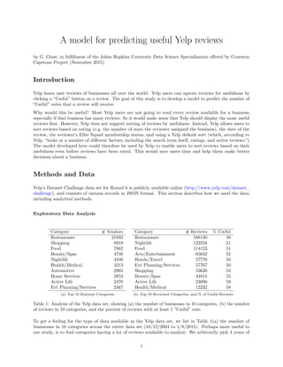
Category # Vendors
Restaurants 21892
Shopping 8919
Food 7862
Beauty/Spas 4738
Nightlife 4340
Health/Medical 3213
Automotive 2965
Home Services 2853
Active Life 2470
Evt Planning/Services 2467
(a) Top 10 Business Categories
Category # Reviews % Useful
Restaurants 588130 49
Nightlife 123558 51
Food 114123 51
Arts/Entertainment 65632 52
Hotels/Travel 57776 50
Evt Planning/Services 57767 50
Shopping 53626 53
Beauty/Spas 34815 55
Active Life 23090 59
Health/Medical 12232 58
(b) Top 10 Reviewed Categories, and % of Useful Reviews
Table 1: Analysis of the Yelp data set, showing (a) the number of businesses in 10 categories, (b) the number
of reviews in 10 categories, and the percent of reviews with at least 1 "Useful" vote.
To get a feeling for the type of data available in the Yelp data set, we list in Table 1(a) the number of
businesses in 10 categories across the entire data set (10/12/2004 to 1/8/2015). Perhaps more useful to
our study, is to find categories having a lot of reviews available to analyze. We arbitrarily pick 4 years of
1

2. data covering 2010 through 2013, and summarize the number of reviews across 10 categories in Table 1(b).
To verify a sufficient number of these reviews are useful, we also list in Table 1(b) the percent of reviews
receiving at least 1 “Useful” vote. The data shows a nice balance between useful and non-useful reviews.
Note that a “Useful” vote here is a positive non-negative integer representing count data, with a mean of 1.1
and a range of 0 to 166. We use the data described in Table 1(b) for all of our work below.
Analytical Methods
We chose the following subset of features from the Yelp data set as potential predictors for our model.
Table 2: Potential features to predict the usefulness of reviews
Yelp Data Set Feature Description
Business stars The number of stars assigned to a business by a review.
Review text_length The number of characters in the review text.
Review votes_funny_review The number of “Funny” votes the review received.
Review votes_cool_review The number of “Cool” votes the review received.
User num_friends The number of friends a reviewer has.
User years_elite The number of years the reviewer has been an Elite Squad member.
User fans The number of fans a reviewer has.
User review_count The total number of reviews made by the reviewer.
User votes_funny_user The number of “Funny” votes the reviewer received.
User votes_cool_user The number of “Cool” votes the reviewer received.
User votes_useful_user The number of “Useful” votes the reviewer received.
The data is prepared as follows. We first remove from the data set any review whose total text length is too
small, which we arbitrarily determine to be less than 20 characters. We add the ability to programmatically
subset reviews based on business category (e.g. Restaurants). We retain only those reviews falling between
1/1/2010 and 1/1/2014. Feature standardization is then performed, whereby each feature is centered by
subtracting its mean, and scaled by dividing by its standard deviation. This provides a zero-mean unit-variance
distribution for each feature, which tends to help estimators learn from features as expected. Finally, we
randomly select 70% of the data set for training, and 30% for testing. The testing data will be used for cross
validation to help us assess how well a particular model generalizes to an independent data set.
We analyze three different models: (1) linear regression, (2) zero-inflated Poisson regression, and (3)
gradient boosting. Linear regression models the relationship between a scalar dependent variable
(e.g. votes_useful_review) and one or more independent variables (e.g. features in Table 2). The relationship
is modeled using linear predictor functions and is based on least-squares fitting.
We use zero-inflated Poisson regression from the PSCL package, which is noted to be a useful model for
predicting count data with many zeros (from Table 1, roughly half of our data has 0 “Useful” votes). Excess
zeros are modeled independent of non-zero data. The model is thus really two separate models: a Poisson
count model (with log link) for non-zero data, and a logit model for zero data. This model is particularly
useful for predicting outcomes where the underlying cause of zero data is different than for non-zero data.
Finally, we use extreme-gradient boosting (xgbTree) from the caret package, which is a fast and efficient
method of gradient boosting. A form of decision tree learning, xgbTree is based on an iterative process
that runs an optimization algorithm on a cost function. We include it here because it was suggested
(http://startup.ml/blog/xgboost) that boosting is more accurate than random forest, bagging, and single-tree.
Each of these 3 models is applied to predict the number of “Useful” votes a review will receive based on
one or more features above. The model showing the best result will then be used to perform more detailed
analyses on the data. To evaluate model performance, we forgo the usual mean-squared error in favor of
2

3. the root-mean squared log error (RMSLE) shown below, where n is the number of observations, p is the
prediction, and a is the response.
RMSLE =
1
n
n
i=1
(log(pi + 1) − log(ai + 1))2
The advantage of RMSLE (https://www.kaggle.com/wiki/RootMeanSquaredLogarithmicError) is that it can
contribute more error for reviews with less votes. For example, RMSLE assigns more error predicting 4 for an
actual 5 “Useful” votes, versus predicting 99 for an actual 100, which seems a sensible approach for our data.
Both linear regression and extreme-gradient boosting algorithms provide the ability to constrain predictions
within a certain range specified by a predictionBounds property. We experimented with setting this property
to a range of 0 to 166 to prevent negative votes. The algorithms otherwise used their default settings when
applied to the training set. The models created from the training set were then used to predict the number
of “Useful” votes in the test set.
Additionally we use the caret package’s varImp() function to understand the relative importance for each of
the features used to create a model. Depending on the results, we can try to simplify the model by eliminating
unimportant features.
Results
Model Selection
Table 3(a) summarizes the prediction results. The zero-inflated Poisson regression model (zeroinfl) was
observed to have the largest RMSLE error. Results for the other two models were better, although constraining
outcomes via predictionBounds did not have a significant effect on RMSLE error. Plotting residuals produced
a random pattern, indicating unbiased results (good). Overall, the extreme-gradient boosting model xgbtree1
had slightly lower RMSLE errors than the linear regression model lm.
Category zeroinfl lm xgbtree1 xgbtree2
Restaurants 0.46 0.42 0.40 0.41
Nightlife 0.47 0.43 0.41 0.42
Food 0.45 0.42 0.40 0.41
Arts/Entertainment 0.46 0.43 0.42 0.42
Hotels/Travel 0.48 0.45 0.44 0.44
Evt Planning/Services 0.48 0.45 0.43 0.44
Shopping 0.47 0.44 0.42 0.43
Beauty/Spas 0.53 0.51 0.48 0.49
Active Life 0.52 0.49 0.46 0.47
Health/Medical 0.52 0.50 0.47 0.48
(a) RMSLE results for models
Feature Health/Med Food
votes_cool_review 100 100
votes_funny_review 20 9
stars 13 2
votes_useful_user 12 1
text_length 9 2
review_count 5 1
num_friends 3 1
fans 2 0
votes_funny_y 1 0
votes_cool_y 1 0
years_elite 0 0
(b) xgbtree1 feature importance for 2 categories
Table 3: Model analysis showing (a) xgbtree has the least RMSLE error, and (b) the relative importance of
features in xgbtree1 model for 2 example categories. The top 5 features in (b) are used to create xgbtree2.
Table 3(b) lists the relative importance for each of the 11 features used in xgbtree1, for 2 example business
categories (Health/Medical, and Food). For all 10 business categories, votes_cool_review contributed a
relative importance of 100, and votes_funny_review came in second with a range of 8 to 23 of relative
importance. The next 3 features in Table 3(b) (e.g. stars, votes_useful_user, and text_length) varied
in relative importance between 1 and 13 among all categories. Finally, the last 6 features in Table 3(b) were
not very important to the model, having an importance of less than 2, usually much less, except for the
3

4. Health/Medical category. From these results we created a new model xgbtree2 using only the top 5 features
of Table 3(b), and obtained similar RMSLE errors as xgbtree1 as shown in Table 3(a). Based on this data,
the primary model for this study was selected as xgbtree2.
Primary Model Results
Our primary model xgbtree2 is based on an efficient gradient boosting algorithm. The model was optimized
by minimizing the root-mean-squared error (RMSE), while holding the shrinkage factor eta constant at 0.3,
and resampling 25 iterations for bootstrapping. Table 4 lists key model parameters across business categories
based on the training data set, where nrounds is the number of boosting iterations and max_depth is the
maximum tree depth. The R-squared (Rˆ2) value is a goodness-of-fit number, where 1 indicates the model
explains all of the variability of the response data around its mean (good), and 0 indicates the model explains
none of this variability (bad). Corresponding data for the test set appeared similar. For completeness, Table
4 also includes the RMSLE prediction result for the test data set, shown previously in Table 3(a).
Table 4: Summary of xgbtree2 models and RMSLE results across business categories
Category nrounds max_depth RMSE RMSE std dev Rˆ2 Rˆ2 std dev RMSLE
Restaurants 150 2 1.01 0.02 0.73 0.005 0.41
Nightlife 50 3 1.14 0.04 0.71 0.011 0.42
Food 100 2 1.02 0.01 0.74 0.008 0.41
Arts/Entertainment 50 3 1.11 0.01 0.75 0.011 0.42
Hotels/Travel 50 3 1.13 0.02 0.69 0.011 0.44
Evt Planning/Services 50 3 1.13 0.01 0.69 0.015 0.44
Shopping 150 2 1.11 0.03 0.68 0.014 0.43
Beauty/Spas 50 2 1.31 0.03 0.57 0.019 0.49
Active Life 50 2 1.39 0.04 0.64 0.020 0.47
Health/Medical 50 2 1.39 0.07 0.50 0.031 0.48
Figure 1 illustrates our primary model with a boxplot to summarize predictions of “Useful” votes for 588130
Restaurant reviews. The x-axis is the “truth”, or the actual number of “Useful” votes that a particular review
received, and the y-axis is the outcome, or the predicted number of “Useful” votes for that review.
0 2 4 6 8 11 14 17 20 23 26 29 32 35 38 43 47 51 67
01020304050
Figure 1. Primary−model (xgbtree2) prediction results for Restaurants category
Actual # of Useful Votes
Predicted#ofUsefulVotes
4

5. Ideally, we’d like to see the mean value of each box plot fall in a straight diagonal line with a slope of 1. The
data generally reflects this trend, although the mean predicted number of “Useful” votes tends to be slightly
less than the actual number. We also observe that reviews receiving larger numbers of “Useful” votes (to the
right on the x-axis) are rare, giving rise to less accurate predictions, and more variation.
To verify the implication of Table 3(b) that business categories should be modeled separately, we used the
xgbtree2 model derived from the Food category training set to predict the Health/Medical test set, and
confirmed that the RMSLE degraded significantly (from 0.41 to 0.50).
Discussion
Our goal is to predict the number of “Useful” votes that a review will receive. We began by briefly reviewing
3 promising algorithms for this task using 11 different features from the Yelp data set. Roughly half the
reviews had 0 “Useful” votes, and the other half had votes ranging from 1 to 166, with a mean 1.1. The
zero-inflated Poisson regression model zeroinfl proved the least effective, suggesting that the underlying
processes generating zero votes and count data may not be independent. The linear regression model lm
produced consistently better predictions than zeroinfl across all business categories. But ultimately, the
extreme gradient boosting model xgbtree1 provided slightly less errors than lm. Gradient boosting can do a
better job fitting complex nonlinear relationships, which might explain this performance improvement.
From the start, it wasn’t clear whether reviews should be modeled separately by business category. We
devised a strategy to model each category separately, then see if the features’ importance values differed
significantly between categories. Table 3(b) highlights the result of this study for 2 categories. Considering
all categories, only the top 5 features appeared to be important. However, the relative weighting among
these 5 features varied significantly between categories. We therefore decided to retain only these 5 features
in our primary model xgbtree2, and apply this model separately to each business category. After creating
xgbtree2 models from training sets, and generating new predictions for the test sets, we circled back to
verify our understanding – when we applied the model generated from the Food training data to predict test
data from the Health/Medical category, we observed the RMSLE error increase significantly from 0.41 to 0.50.
This suggests some merit to modeling categories separately. Table 3(b) might help us understand why. For
example, it may make sense that the length of text in a review is more important for Health/Medical than
Food reviews. Also, users having higher number of votes for being “Useful” tended to write reviews that got
voted more “Useful”, which might be explained if some users are experts in the medical field and were more
highly valued for their expertise compared with experts in the Food category. This is just speculation though.
Since the predicted number of “Useful” votes is a floating point number, and the actual number of votes is
an integer, one thought to reduce the RMSLE error was to round the predicted result to an integer before
computing RMSLE. In practice, however, this only increased the RMSLE error.
In summary, the primary model xgbtree2 was determined to be extreme gradient boosting with 5 fea-
tures: votes_cool_review, votes_funny_review, stars, votes_useful_user, and text_length. The
votes_cool_review is by far the most important feature, with votes_funny_review a distant second. The
significance of the other features depends on the business category being modeled. The shrinkage factor eta
is 0.3, and the number of resampling interations for bootstrapping is 25. We recommend fitting a model for
each business category separately. The boosting iterations and maximum tree depth varied with business
category from 50 to 150, and 2 to 3, respectively.
Figure 1 shows that the primary model can perform well, although on average it slightly underestimates the
actual number of “Useful” votes. Table 4 lists categories by population from highest to lowest, and generally
speaking the fit degrades as we traverse down the table. The R-squared (Rˆ2) data degrades from 0.73 to 0.5,
and RMSLE increases from 0.41 to 0.48. This suggests the model can learn better given more observations.
This also agrees with the data appearing in the right half of Figure 1, where low populations give rise to
larger errors and variance.
5