1. Introduction
Materials and Methods
Data Analysis & Graphs Results
Literature Cited
Karleskint, G., Turner, R., & Small, J. W. (2010). Introduction to marine biology. Belmont, CA:
Brooks/Cole Cengage Learning.
Perry, R. (2003). A guide to the marine plankton of southern california. UCLA OceanGlobe, 3, 03-09.
Dube, A., Jayaraman, G., & Ran, R. (2010). Modelling the effects of variable salinity on the temporal
distribution of plankton in shallow coastal lagoons.Journal of Hydro-environment
Research, 4, 199-209.
Vertical Distribution of Plankton in
Possession Sound
By: Bryan Jacobson and Breanne Ward
The Ocean Research College Academy, (ORCA) is a one-of-
a-kind running start program designed for high school juniors and
seniors who are interested in learning through intensive studies based
in the local estuary. Every four weeks the students of ORCA organize
and complete a State of Possession Sound (SOPS) cruise. The
students visit two or three stations each to observe the organisms
present in the area, along with taking numerous chemical
measurements of data to track the state of the Sound over time. With
plankton holding the lowest position of the marine food chain, the
abundance of plankton within Possession Sound is a key factor to its
health and stability. Phytoplankton also has an irreplaceable role in the
biogeochemical cycle of the atmosphere, recycling and reusing carbon
within the atmosphere (Karleskint, Turner, & Small, 2010). In an
attempt to better understand the lifestyle and habits of plankton, an
experiment was conducted to gather data concerning planktons’
location within the vertical water column, with regards to the depth of
the halocline. The hypothesis suggests that a higher percentage of
plankton will reside at or above the halocline due to either the varying
density gradients that contribute to vertical stratification, trapping the
plankton in the higher areas of the water, or the higher levels of
nutrients and sunlight available in the surface layer.
Research was conducted using a Niskin bottle to gather 1.2
liter samples at three different depths within the water column. A YSI
650 was used to determine the halocline of the water, and samples
were then taken from three meters above the halocline, directly at the
halocline, and three meters below it. The water samples were brought
to the surface and poured through a 250 μm plankton net to filter out
whatever plankton was caught (figure #8), which was then poured into
a separate labeled bottle to be preserved with Formalin and dyed with
Lugol’s solution for counting. To count the plankton the samples were
left to settle overnight before a pipette was used to collect a 5 milliliter
bottom sample, taking in as much plankton as possible. The pipette
was then again left to settle until the accumulated plankton had sunk to
the bottom. The bottom 1 milliliter portion of plankton was then used
for identification and counting (figures #9 and #10).
After identifying and counting plankton samples from three
different locations within Possession Sound, the results have
successfully supported our hypothesis. A higher percentage of the
total plankton was counted at or above the determined halocline, than
below. At the first station, Mount Baker Terminal, out of the 2,223
plankton counted, 82.3% were at/above the halocline. At the second
station, Dolphin, 91.2% were at/above the halocline; and at the third
station, Buoy, 75.09% were counted at/above the halocline, giving an
average of 82.86% of plankton being at or above the determined
halocline of the water. 21 different species of plankton were identified
throughout all samples, including 16 phytoplankton species and 5
zooplankton species. The most abundant species overall was
Thalassiosira pseudonana, closely competing with the second most
common species counted, Skeletonema costatum.
0
50
100
150
200
250
300
350
400
450
500
550
TotalCounted
Figure #1
Mount Baker Terminal Plankton Populations
Above Cline
At Cline
Below Cline
0
50
100
150
200
250
300
350
400
450
500
550
Totalcounted
Figure #2
Dolphin Plankton Populations
Above Cline
At Cline
Below Cline
0
50
100
150
200
250
300
350
400
450
500
550
TotalCounted
Figure #3
Buoy Plankton Populations
Above cline
At Cline
Below Cline
Figures #1-3 depict the total plankton abundance by species for each site. Although all 3 stations fully support our hypothesis regarding the
vertical distribution of plankton in relation to the halocline, it can still be seen that there are differences in the concentration of plankton at each site.
Figure #1 shows the species distribution above, at and below the halocline of the station Mount Baker Terminal. Comparing this graph to those of
stations #2 and #3 (figures #2 and #3) it can be seen that the area of the water column containing the greatest abundance of plankton varies by
station. At Mount Baker Terminal the greatest aggregation of plankton is located approximately 2-3 meters above the halocline, compared to the
stations Dolphin or Buoy, who both have a larger concentration of plankton directly at the halocline. This difference could potentially be a result of the
location of the halocline at those stations. The halocline at Mount Baker Terminal was the closest to the surface compared to the other two stations (2
meters down versus roughly 3-4).
This difference in plankton concentration could also be a result of the varying levels of surface salinity at each location. The surface salinity at
Mount Baker Terminal (22.16 ppt.) was much higher than those at both Dolphin and Buoy, (17.05 and 12.33 ppt.). Different species of plankton
sometimes survive better in higher/lower levels of salinity, (Dube, Jayaraman, & Ran, 2010) and will aggregate in those levels, thus leading into the
possibility that the planktons were potentially lower in the water column at the 2nd and 3rd stations due to the fact that the surface salinity levels were
so low, possibly as a result of the recent rain storms and lack of sunshine and evaporation. This would imply that the plankton might not congregate
specifically at the halocline, but instead, congregate within a specific range of salinity (between roughly 22-24 ppt. in this case). It just happens to
occur that the levels of salinity at the surface of Mount Baker Terminal are fairly close to the levels of salinity that occur at the halocline of the stations
Dolphin and Buoy, explaining the reasoning for the Halocline being the most populated region in the stations Buoy and Dolphin, and the above-cline
region being the most abundant at Mount Baker Terminal (figure #4).
The two most common types of phytoplankton detected were Thalassiosira pseudonana and Skeletonema costatum (figures #5 and #6). The
vast abundance of both species at all 3 stations could possibly be related to their shared characteristic of both being chain diatoms. Chain diatoms
are relatively large compared to other phytoplankton, and have a larger Reynolds Number as a result of their expanded surface area. This increase in
surface area contributes to the buoyancy of the plankton, allowing them to easily remain in the surface area of the water without sinking below it, as
many smaller phytoplankton do.
Conclusion
The data collected supports the hypothesis of increased
plankton populations at or above the halocline potentially due to the
density stratification between the lower and higher salinity layers of the
water column, or the higher levels of nutrients and sunlight.
In future research it would be interesting to look into the
pycnocline of each of the station as well as tracking the seasonal
variance of plankton abundance and species distribution throughout
the year. It could potentially be beneficial to incorporate a chlorophyll
sensor into further research in order to gather complimentary data on
phytoplankton concentrations.
Dolphin
Buoy
MBT
0
200
400
600
800
1000
1200
Above Halocline
At Halocine
Below Halocline
Station
TotalPlanktonCounted
Location
Total Plankton Abundance by Station and Relative Depth
Dolphin
Buoy
MBT
Figure #4
Figure #5
Halocline Depth by Station
Figure #6 Figure #7
Figure #8
Figure #9 Figure #10