1. Analyzing Baseball
Anthony Spina and Max Steinhorn
November 21, 2014
Stats 111-03 Final Project
Introduction
Amherst College has a long tradition of sending its alumni to the front offices of Major League Baseball teams.
Currently, the Red Sox, Pirates, and Orioles have Amherst alums calling the shots as General Managers. All
three have sent their team to the playoffs in recent years – and we are trying to find how they did it. What
statistics correlate strongly with wins, and therefore playoff appearances? What should a General Manager
focus on when looking for players in Free Agency? Is there a regression line that will best model how teams
make the playoffs? Are some statistics significantly different on playoff teams and non-playoff teams? We
looked at many offensive and defensive statistics of all Major League teams in the 2014 season to help us
answer these questions.
Data
This data includes a lot of traditional and progressive (sabermetric) offensive and pitching statistics in
baseball. It also includes payroll in millions and wins for each team and whether the teams play in a pitcher
or hitter friendly ballpark. Most people are familiar with the traditional statistics of HR, R, RBI, SB, AVG,
strikeout percentage, walk percentage, ERA, and payroll. But some statistics that are not well known are
OPS, WAR, WHIP, and how to determine what kind of ballpark a team plays in. OPS is a statistic that adds
the OBP (how often one gets on base) with SLG (a measure of power that divides total bases by at-bats).
WAR, is a complicated but very powerful statistic. It combines many attributes of baseball to determine
a person’s impact on the team. WAR is the summation of how many runs a player scores on offense and
prevents on defense divided by how many runs it takes to win a game. An individual WAR of 2 or 3 is a solid
starter for a team, while a WAR of 7 is an MVP caliber player. WHIP is a pitching statistic that calculates
walks and hits per innings pitched. To determine if a ballpark is pitcher or hitter friendly, you compare the
runs scored and allowed at home with runs scored and allowed on the road. A statistic over 1 yields a hitters
park and below 1 yields a pitchers park. It is our job to sift through the data and decide which statistics –
traditional, sabermetric, or both – help teams win games and ultimately make the playoffs.
Here is a preview of our data:
## HR R RBI SB BB. K. AVG OPS WAR Payroll Wins ERA WHIP
## Dodgers 134 718 686 138 8.3 20.0 0.265 0.739 31.2 235.29 94 3.40 1.21
## Angels 155 773 729 81 7.8 20.1 0.259 0.728 30.3 155.69 98 3.58 1.22
## Orioles 211 705 681 44 6.5 21.0 0.256 0.733 29.0 107.41 96 3.43 1.24
## Pirates 156 682 659 104 8.4 20.0 0.259 0.734 26.9 78.11 88 3.47 1.26
## Nationals 152 686 635 101 8.3 21.0 0.253 0.714 25.4 134.70 96 3.03 1.16
## Giants 132 665 636 56 7.0 20.5 0.255 0.699 23.7 154.19 88 3.50 1.17
## K.9 Park FPct
## Dodgers 8.44 Pitcher 0.983
## Angels 8.15 Pitcher 0.986
## Orioles 8.03 Pitcher 0.986
## Pirates 7.59 Pitcher 0.983
## Nationals 7.88 Hitter 0.984
## Giants 7.52 Pitcher 0.984
1

2. There are some interesting graphs we can visualize right away just by taking a few of the variables from our
dataset:
Scatter Plot Matrix
WAR20
30
20 30
10
2010 20
OPS0.70
0.74
0.70
0.64
0.680.64
Wins80
90
80 95
65
7565 80
ERA4.0
4.5
4.0
3.0
3.5
3.0
WHIP1.30
1.40
1.30
1.15
1.251.15
With many of our earlier regressions, we dealt with the issue of colinearity, which is to say that many of our
explanatory variables were strongly correlated with each other. This graph above shows us that perhaps there
is a bit of colinearity amongst categories of the same category (offensive or defensive). For our regression, we
tried to pick variables that correlated well with Wins, but that didn’t necessarily strongly correlate with any
other variables. This matrix was really helpful in doing so because it allowed us to take a large-scale look at
our graphs and determine which variables would be helpful in our dataset.
In order to compare a lot of the different data we have in this dataset, one thing we will use is a T-test to
compare two different means. Below you will find that we’re added a new column to our dataset, displaying a
True or False statement signifying whether or not the team was a playoff team.
In case you want to look at the data to get an idea of our dataset:
## HR R RBI SB BB. K. AVG OPS WAR Payroll Wins ERA WHIP
## Dodgers 134 718 686 138 8.3 20.0 0.265 0.739 31.2 235.29 94 3.40 1.21
## Angels 155 773 729 81 7.8 20.1 0.259 0.728 30.3 155.69 98 3.58 1.22
## Orioles 211 705 681 44 6.5 21.0 0.256 0.733 29.0 107.41 96 3.43 1.24
## Pirates 156 682 659 104 8.4 20.0 0.259 0.734 26.9 78.11 88 3.47 1.26
## Nationals 152 686 635 101 8.3 21.0 0.253 0.714 25.4 134.70 96 3.03 1.16
## Giants 132 665 636 56 7.0 20.5 0.255 0.699 23.7 154.19 88 3.50 1.17
## K.9 Park FPct playoffs
## Dodgers 8.44 Pitcher 0.983 TRUE
## Angels 8.15 Pitcher 0.986 TRUE
## Orioles 8.03 Pitcher 0.986 TRUE
## Pirates 7.59 Pitcher 0.983 TRUE
## Nationals 7.88 Hitter 0.984 TRUE
## Giants 7.52 Pitcher 0.984 TRUE
We decided to do four different T-tests in R to compare specific means that we care about. We wanted to see
whether there was a significant difference in the mean statistics of playoff and non-playoff teams. Out of the
30 teams in our dataset (and in the Major Leagues) 10 made the playoffs. To do this T-test, we need to check
a few assumptions. First our data should be independent (between groups and within groups). We would
like our data to pass the Randomization Condition and the 10% Condition, but we are using all teams–so
we do not pass the 10% Condition or the randomization condition. We are aware of this and will proceed
with caution. We also check the Nearly Normal condition by looking at the histogram of our population (for
2

3. playoff and for non-playoff teams) and it was normal. We do have issues with the independent assumption
because each team plays each other, but as with the independence assumption, we will proceed with caution.
This first T-test is comparing the statistical sabermetric WAR (which is an attempt to measure the total
contribution of each player for each individual team in one statistic) for teams who made the playoffs with
teams who did not.
##
## Welch Two Sample t-test
##
## data: WAR by playoffs
## t = -7.411, df = 21.29, p-value = 2.518e-07
## alternative hypothesis: true difference in means is not equal to 0
## 95 percent confidence interval:
## -13.111 -7.369
## sample estimates:
## mean in group FALSE mean in group TRUE
## 15.58 25.82
Since zero is not within the 95% confidence interval, we can reject the null hypothesis and say that the mean
WAR of playoff teams is significantly different (higher for group TRUE) than the mean WAR of non-playoff
teams.
We wanted to test this same strategy with the offensive category of OPS (On-Base Percentage Plus Slugging):
##
## Welch Two Sample t-test
##
## data: OPS by playoffs
## t = -2.826, df = 22.41, p-value = 0.009733
## alternative hypothesis: true difference in means is not equal to 0
## 95 percent confidence interval:
## -0.048181 -0.007419
## sample estimates:
## mean in group FALSE mean in group TRUE
## 0.6906 0.7184
Again our variable of OPS seems to be statistically significant within a 95% confidence interval. We can reject
the null hypothesis because zero isn’t in our confidence interval. Although OPS is statistically significant
(higher for playoff teams than non-playoff teams), there may not be reason to believe that it is practically
significant since the upper bound of the confidence interval is very close to zero.
Another T-test, this time for payroll:
##
## Welch Two Sample t-test
##
## data: Payroll by playoffs
## t = -1.391, df = 15.49, p-value = 0.184
## alternative hypothesis: true difference in means is not equal to 0
## 95 percent confidence interval:
## -61.72 12.90
## sample estimates:
## mean in group FALSE mean in group TRUE
## 107.0 131.4
3

4. With our 95% confidence interval, it seems as if this is not statistically significant because our width contains
zero, so we fail to reject the null hypothesis. We can note that there doesn’t seem to be a relationship for
payroll between teams that are in the playoffs and teams that are not.
For our last T-test, we will compare ERA for teams that did and did not make the playoffs:
##
## Welch Two Sample t-test
##
## data: ERA by playoffs
## t = 3.201, df = 27.46, p-value = 0.003443
## alternative hypothesis: true difference in means is not equal to 0
## 95 percent confidence interval:
## 0.1473 0.6717
## sample estimates:
## mean in group FALSE mean in group TRUE
## 3.874 3.465
ERA seems to be statistically significant with a 95% confidence interval. We can reject the null hypothesis,
because zero isn’t in our confidence interval, although it is very close. Perhaps there is reason to believe that
although it is statistically significant, it may not be practically significant.
Another thing we wanted to explore was how to predict if a team is expected to make the playoffs. In order
to even think about fitting a regression with variables, we wanted to first see what the average amount of
wins in 2014 for playoff team was. To do so, we made a 95% confidence interval for teams in the playoffs:
## mean of x lower upper level
## 91.70 88.92 94.48 0.95
Using this data as a model, we are 95% confident that the true mean wins for playoff teams is between 89 and
94.5 wins. In order to model for wins, we would expect, on average, a playoff team to be within this range.
Now it is time for us to come up with a model to predict for wins. We know how many wins are desired on
average to make the playoffs. For our dataset, we have made a model using the seemingly best variables
found, hoping to increase the variablility of our model while hoping to keep a low p-value for each variable
involved. In order to create a model, though, we need to check a few assumptions. For a multiple regression
we need to check “LINE”. We pass the linearity condition with the scatterplot graph of Wins against our
fitted model. The next condition has to do with independence, which as we mentioned earlier, we have not
completely satisfied. For the Nearly Normal Condition, we checked a histogram of the residuals and it was
normal. We can check the equal variance condition by checking a scatterplot of the residuals against the
fitted. The plot does not thicken–and the assumption is satisfied.
Our first model is as follows:
lm2 <- lm(Wins ~ WAR + OPS + WHIP + ERA, data=y)
summary(lm2)
##
## Call:
## lm(formula = Wins ~ WAR + OPS + WHIP + ERA, data = y)
##
## Residuals:
## Min 1Q Median 3Q Max
## -6.214 -2.247 -0.202 1.852 6.346
4

5. ##
## Coefficients:
## Estimate Std. Error t value Pr(>|t|)
## (Intercept) 52.052 26.781 1.94 0.0633 .
## WAR 0.381 0.250 1.53 0.1391
## OPS 125.624 48.739 2.58 0.0162 *
## WHIP -5.367 23.564 -0.23 0.8217
## ERA -15.883 4.296 -3.70 0.0011 **
## ---
## Signif. codes: 0 '***' 0.001 '**' 0.01 '*' 0.05 '.' 0.1 ' ' 1
##
## Residual standard error: 3.61 on 25 degrees of freedom
## Multiple R-squared: 0.878, Adjusted R-squared: 0.859
## F-statistic: 45 on 4 and 25 DF, p-value: 4.51e-11
We picked these variables because they seemed to correlate the best with our original Splom matrix graph.
However, in the summary of this regression, you can notice that the p-values for both WAR and WHIP are
high. While the p-value for WAR doesn’t seem extremely high, it is higher than our desired alpha level of .05.
Even though our T-tests above show that the WAR among playoff teams are higher than nonplayoff teams, it
doesn’t seem like this variable fits well inside of our regression model.
Taking out WAR and WHIP, we are left with our final linear regression:
lm3 <- lm(Wins ~ OPS + ERA, data=y)
summary(lm3)
##
## Call:
## lm(formula = Wins ~ OPS + ERA, data = y)
##
## Residuals:
## Min 1Q Median 3Q Max
## -6.701 -2.005 -0.813 2.380 8.378
##
## Coefficients:
## Estimate Std. Error t value Pr(>|t|)
## (Intercept) 21.22 15.82 1.34 0.19
## OPS 193.18 23.68 8.16 9.3e-09 ***
## ERA -20.18 1.64 -12.31 1.4e-12 ***
## ---
## Signif. codes: 0 '***' 0.001 '**' 0.01 '*' 0.05 '.' 0.1 ' ' 1
##
## Residual standard error: 3.66 on 27 degrees of freedom
## Multiple R-squared: 0.865, Adjusted R-squared: 0.855
## F-statistic: 86.3 on 2 and 27 DF, p-value: 1.87e-12
We chose to pick the offensive category and the pitching category that gave us the highest variability for the
model while also maintaining a low p-value below .05. As you can see, our two p-values are well below that
mark. Hitting and pitching categories are independent of each other, so we avoided any colinearity. ERA
measures the amount of earned runs a pitcher gives up (runs he gives up discarding the ones because of
errors) every 9 innings. OPS is an offensive measure of total bases per at bat. This model seems to pass all
of the assumptions – independence, linearity, normal residuals, and equal variance.
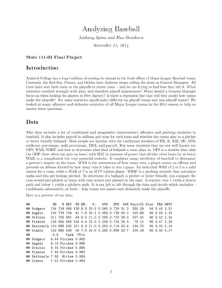
Another imporant graph for this regression can be found below:
5

6. fitted(lm3)
Wins
70
80
90
70 80 90
This graph is super important for our project because it shows us that there is a strong, positive linear
regression for our model. This graph is does an awesome job illustrating the exactly how well Wins correlates
with our regression. There doesn’t seem to be any immediate concern over any outliers, but that is just
something we should probably just always keep in mind.
Another graph we should look at to ensure there are no immediate concerns is the graph of the residuals
against the fitted linear model:
fitted(lm3)
residuals(lm3)
−5
0
5
70 80 90
The graph of the residuals looks good. The red line is just separating the data (at residuals = 0) so its easier
to view. The plot definitely doesn’t thicken and there doesn’t seem to be any huge points of concern–so
that’s good!
Below is a box plot displaying the relationship between wins and the different types of Stadium (hitter or
pitcher friendly Ballpark):
6

7. Wins
70
80
90
Hitter Pitcher
##
## Welch Two Sample t-test
##
## data: Wins by hitters
## t = 1.715, df = 27.88, p-value = 0.09749
## alternative hypothesis: true difference in means is not equal to 0
## 95 percent confidence interval:
## -1.122 12.640
## sample estimates:
## mean in group FALSE mean in group TRUE
## 84.07 78.31
While looking at the boxplot, it would seem logical to conclude that teams that play in a “pitcher’s park”,
have on average more wins.
As we can see with this T-test, the confidence interval includes zero, and so there is not a statistically
significant mean amount of wins. Although it seemed like the data was statistically significant when looking
at the boxplots, using a two-Sample T-test proved otherwise.
Conclusion
Our findings in dealing with this dataset yields some interesting conclusions. First, we are 95% confident
teams that make the playoff will have on average, 89 to 95 wins. Next, we fitted a multiple regression
model, using ERA and OPS, that best describes wins. Lastly, we computed multiple t-tests to see whether
statistics for playoff teams and non-playoff teams were statistically different. We found that while playoff
teams have significantly higher WAR, ERA, and OPS, both ERA and OPS may not be practically significant.
We also found that a team’s payroll for playoff and non-playoff teams was not significantly different. Our
processes, however, were not without flaws. We did not pass the independence assumption for our confidence
intervals, regression models, and t-tests. Perhaps we could have expanded our dataset to include more
complex sabermetric statistics or even to include multiple years of data. Although we could never fully fulfill
the independence assumptions, we could perhaps minimize the negative effects by expanding our dataset.
7