1) The document discusses derivatives as rates of change, using the example of a stone thrown straight up.
2) It is found that the stone will stay in the air for 6 seconds, reaching its maximum height of 144 feet after 3 seconds.
3) The derivative of the height function D(t) represents the instantaneous rate of change of height, or speed, at each time t. This rate varies throughout the stone's trajectory.
The document discusses quadratic functions and parabolas. It defines quadratic functions as functions of the form y = ax2 + bx + c, where a ≠ 0. It states that the graphs of quadratic equations are called parabolas. Parabolas are symmetric around a central line, with the vertex (highest/lowest point) located on this line. The vertex formula is given as x = -b/2a. Steps for graphing a parabola are outlined, including finding the vertex, another point, and reflections across the central line. An example graphs the parabola y = x2 - 4x - 12, finding the vertex as (2, -16) and x-intercepts as -
This document discusses rules for computing derivatives of functions. It begins by listing existing derivative rules and defining notation. It then derives and presents rules for the derivatives of trigonometric functions like sine, cosine, tangent, cotangent, secant and cosecant. An example problem demonstrates finding the derivative of the tangent function using previous rules.
Este documento describe el uso del software Geogebra para visualizar y animar conceptos topológicos como espacios métricos, distancias, bolas abiertas y cerradas. Incluye ejemplos interactivos de distancias euclídeas y no euclídeas en R2 y R, y muestra cómo Geogebra puede ayudar a comprender intuitivamente nociones abstractas a través de su materialización en un entorno virtual.
Este documento presenta ejercicios sobre operaciones con expresiones algebraicas fraccionarias. Incluye problemas de factorización, simplificación, multiplicación, división, adición y sustracción de fracciones algebraicas, así como determinación de mínimos comunes múltiplos y resolución de ejercicios combinados.
The document discusses functions and their basic language. It defines a function as a procedure that assigns each input exactly one output. It provides examples of functions, such as a license number to name function. It explains that a function must have a domain (set of inputs) and range (set of outputs). Functions can be represented graphically, through tables of inputs and outputs, or with mathematical formulas.
This document defines functions and related terminology such as domain, codomain, range, one-to-one functions, onto functions, and bijections. It provides examples of graphical representations of functions and discusses concepts like whether a function is one-to-one or onto based on its graph. The pigeonhole principle is also introduced as stating that if more items are put into fewer containers, at least one container must hold multiple items.
The document discusses using sign charts to solve polynomial and rational inequalities. It provides examples of solving inequalities by setting one side equal to zero, factoring the expression, drawing the sign chart, and determining the solutions from the regions with the appropriate signs. Specifically, it works through examples of solving x^2 - 3x > 4, 2x^2 - x^3/(x^2 - 2x + 1) < 0, and (x - 2)/(2/(x - 1)) < 3.
This document discusses first degree functions and linear equations. It explains that most real-world mathematical functions can be composed of algebraic, trigonometric, or exponential/log formulas. Linear equations of the form Ax + By = C represent straight lines that can be graphed by finding the x- and y-intercepts. If an equation contains only one variable, it represents a vertical or horizontal line. The slope-intercept form y = mx + b is introduced, where m is the slope and b is the y-intercept. Slope is defined as the ratio of the rise over the run between two points on a line.
The document discusses related rates problems. It begins by using resizing a rectangle on a computer screen as an example to demonstrate how the rates of change of the length (L) and width (W) relate to the rate of change of the area (A). The key steps are: (1) the area A is given by A=LW, (2) take the derivative of both sides, (3) use the product rule and chain rule to obtain A'=L'W+LW', (4) plug in the given rates of L' and W' to solve for A'.
The document then provides examples to demonstrate how to set up and solve related rates problems by translating the given rates into derivatives, applying
The document discusses Cartesian products, domains, ranges, and co-domains of relations and functions through examples and definitions. It explains that the Cartesian product of sets A and B, written as A×B, is the set of all ordered pairs (a,b) where a is an element of A and b is an element of B. It also defines what constitutes a relation between two sets and provides examples of relations and functions, discussing their domains and ranges. Arrow diagrams are presented to illustrate various functions along with questions and their solutions related to relations and functions.
Las funciones se pueden clasificar como pares, impares o sin paridad según ciertas relaciones de simetría. Una función es par si f(x)=f(-x) y es impar si f(x)=-f(-x). Las funciones pares son simétricas respecto al eje y y las funciones impares tienen simetría rotacional de 180 grados. La suma, producto y cociente de funciones pares o impares también son pares o impares dependiendo de las funciones involucradas.
Notes solving polynomials using synthetic divisionLori Rapp
This document discusses using synthetic division to evaluate polynomials at specific values and factor polynomials. It provides examples of using synthetic division to:
1) Evaluate polynomials like f(x) = x^2 - x + 5 at specific values such as f(-2)
2) Factor polynomials when one factor is known, such as factoring x^3 - 3x^2 - 13x + 15 after determining (x + 3) is a factor
3) Find all zeros of a polynomial by setting each factor equal to 0 after factoring
Step-by-step instructions and additional examples are provided to illustrate the process.
The document discusses properties of derivatives and how they relate to limits. It states that the sum, difference, and constant multiple rules for limits directly apply to differentiation. However, the product and quotient rules for limits do not directly apply to differentiation, which has more complicated product and quotient rules. Elementary functions are defined in terms of a few basic formulas and operations. The document then examines the sum and constant multiple rules for derivatives in more detail, proving them using limits. It also provides a geometric illustration of how the derivative of a sum is equal to the sum of the derivatives.
In this tutorial, we study various statistical problems such as community detection on graphs, Principal Component Analysis (PCA), sparse PCA, and Gaussian mixture clustering in a Bayesian framework. Using a statistical physics point of view, we show that there exists a critical noise level above which it is impossible to estimate better than random guessing. Below this threshold, we compare the performance of existing polynomial-time algorithms to the optimal one and observe a gap in many situations: even if non-trivial estimation is theoretically possible, computationally efficient methods do not manage to achieve optimality. This tutorial will present how we adapted the tools and techniques from the mathematical study of spin glasses to study high-dimensional statistics and Approximate Message Passing (AMP) algorithm.
This tutorial was presented by Marc Lelarge at the 21st INFORMS Applied Probability Society Conference (2023)
https://informs-aps2023.event.univ-lorraine.fr/
Este documento presenta definiciones y propiedades de estructuras algebraicas como conjuntos, operaciones, semigrupos, monóides, grupos, anillos y cuerpos. Introduce conceptos como clausura, asociatividad, elemento neutro e inverso. Explica las propiedades que deben cumplir estas estructuras algebraicas y provee ejemplos ilustrativos.
Este documento describe las propiedades de las funciones logarítmicas. Explica que una función logarítmica tiene la forma f(x)=loga(x) donde a es la base y que la constante a se llama base de la función. También describe que el dominio es los reales, la gráfica es asintótica al eje y y corta el eje x en 1 y 0.
The document discusses factorable polynomials and graphing them. It defines a factorable polynomial P(x) as one that can be written as the product of linear factors P(x) = an(x - r1)(x - r2)...(x - rk), where r1, r2, etc. are the roots of P(x). It explains that for large values of |x|, the leading term of P(x) dominates so the graph resembles that of the leading term, while near the roots other terms contribute to the shape of the graph. Examples of graphs of polynomials like x^n are provided to illustrate the approach.
The document discusses finding the inverse of a function. It defines an inverse function as one that reverses another function by mapping the output back to the input. To find the inverse, you replace the function notation with the output variable, switch the input and output variables, solve for the output variable, and replace it with inverse function notation. Finally, you should check your work.
The document discusses various transformations that can be performed on graphs of functions, including vertical translations, stretches, and compressions. Vertical translations move the entire graph up or down by adding or subtracting a constant to the function. Stretches elongate or compress the graph vertically by multiplying the function by a constant greater than or less than 1, respectively. These transformations can be represented by modifying the original function in a way that corresponds to the geometric transformation of its graph.
Este documento presenta un capítulo sobre funciones de varias variables. Introduce conceptos como funciones vectoriales, escalares y curvas. Explica cómo graficar funciones de dos variables y define el dominio de una función escalar. Proporciona ejemplos de funciones de dos variables y cómo determinar su dominio natural analizando la regla de correspondencia y la forma de su gráfico. El objetivo es conceptualizar estas funciones, describir conjuntos de niveles, establecer límites, continuidad y derivadas.
Este documento contiene ejercicios propuestos sobre límites matemáticos. Se dividen en 10 secciones con ejercicios que calculan límites, evalúan funciones, determinan si un límite existe o no cuando el argumento se acerca a cierto valor, y otros conceptos relacionados con límites. Las secciones contienen entre 1 y 41 ejercicios cada una con soluciones numéricas, funciones o indicaciones de si el límite existe o no.
Este documento explica las funciones cuadráticas de segundo grado. Define una función cuadrática como y=ax2+bx+c y describe cómo la orientación de la parábola depende del signo de a. Explica cómo calcular el vértice de una función cuadrática a partir de sus coeficientes y cómo determinar los puntos de corte con los ejes. Finalmente, muestra un ejemplo completo de representar gráficamente una función cuadrática dada su ecuación.
This document provides an introduction to functions and their properties. It defines what a function is as a mapping from a domain set to a codomain set, and introduces related concepts like domain, codomain, range, and the notation for functions. It then gives examples of specifying functions explicitly and with formulas. The document discusses properties of functions like injectivity, surjectivity, and being increasing or decreasing. It provides examples of determining if a function has these properties. The document concludes by introducing the concept of the inverse function for bijective functions.
Trabajo practico de inecuaciones. 2 año de secundariaRita Oyola
El documento presenta una serie de problemas de álgebra que involucran resolver inecuaciones y determinar cuáles ecuaciones son equivalentes a otras dadas. Se piden resolver 8 inecuaciones, identificar cuáles de 4 ecuaciones son equivalentes a x - 2 ≤ 10, y determinar cuál de 4 ecuaciones es equivalente a -4x ≤ -3x - 5.
COMMENT AND FOLLOW FOR MORE COURS : MATHS , PHILOSOPHIE , PHYSIQUE , PROGRAMMATION PASCAL , BASE DE DONNEES ..
RESUMER DE COURS JOIGNABLE .. 2000-2017 DE BAC INFORMATIQUE 'INFO'
COMMENT AND FOLLOW FOR MORE COURS : MATHS , PHILOSOPHIE , PHYSIQUE , PROGRAMMATION PASCAL , BASE DE DONNEES ..
RESUMER DE COURS JOIGNABLE .. 2000-2017 DE BAC INFORMATIQUE 'INFO'
Le document contient l'énoncé de l'épreuve de modélisation mathématiques.informatique pour la banque d'écoles Agro/Véto 2017. La correction se trouve sur le même site.
Les étapes de la fabrication du ciment soufiane merabti soufiane merabti
for buy this slide : https://payhip.com/b/tMjW
Les étapes de la fabrication du ciment soufiane merabti
Objectifs:
•Acquérir des Connaissances techniques.
•Initiationstechnologique de fabrication des ciments (Processus de fabrication).
•Connaitre le rôle et le fonctionnement des principaux équipements de fabrication des ciments.
Module 01: Processus de fabrication : (Durée : 05 jours) Généralités. Historique du ciment. Différentes étapes de fabrication du ciment. Lecture d'un flow-sheet. Différents procédés de fabrication. Exploitation des carrières. Carrière calcaire. Carrière argile. Matières de correction. Préparation du cru. Pré-homogénéisation. Broyage cru. Homogénéisation. Cuisson. Refroidissement. Transport et stockage du clinker. Broyage clinker. Stockage ciment. Expéditions.
Point sur l'énergie solaire
Historique
Soleil et énergie solaire
L’exploitation de l’énergie solaire dans les
centrales solaires et dans les transports
L’énergie solaire dans les transports et sur les satellites
Programme de l’énergie solaire en Algérie
Programme d’efficacité énergétique en
Algérie
géneralité sur le mecanique de fluide :
Definition d'un fuild
Les grands principes de la mécanique des fluides
Les applications de la mécanique des fluides
TP: calcule le débit volumique d’un écoulement
- Généralité sur les moteurs deux temps
Fonction des defferentes piece du moteur 2 temps
Le cycle moteur 2 temps
Le refroidissement de moteur 2 temps
-Les différents types de moteurs
Les moteurs à injection indirecte
Les moteurs à injection directe
-Le circuit d'alimentation
Pompe d'alimentation
L'élément filtrant
les injecteurs
- Conclusion
For buy this book https://payhip.com/b/CBfA
Fabrication mecanique :
Principe de tournage
Montre cylindre dans un mandrin
Position isostatique
Les différentes cotes de fabrication
Transferts de cotes
TD - travaux dirigé etude de fonction ( exercice ) Soufiane MERABTI
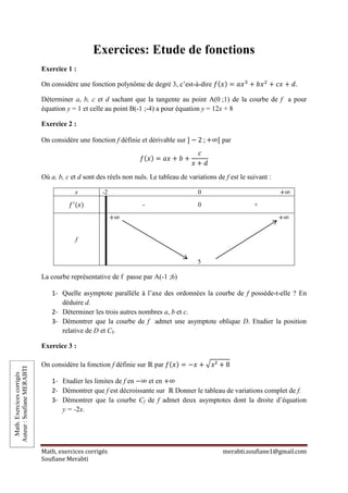
1. Math, exercices corrigés merabti.soufiane1@gmail.com
Soufiane Merabti
Exercices: Etude de fonctions
Exercice 1 :
On considère une fonction polynôme de degré 3, c’est-à-dire ( ) .
Déterminer a, b, c et d sachant que la tangente au point A(0 ;1) de la courbe de f a pour
équation y = 1 et celle au point B(-1 ;-4) a pour équation y = 12x + 8
Exercice 2 :
On considère une fonction f définie et dérivable sur par
( )
Où a, b, c et d sont des réels non nuls. Le tableau de variations de f est le suivant :
x -2 0
( ) - 0 +
f
5
La courbe représentative de f passe par A(-1 ;6)
1- Quelle asymptote parallèle à l’axe des ordonnées la courbe de f possède-t-elle ? En
déduire d.
2- Déterminer les trois autres nombres a, b et c.
3- Démontrer que la courbe de f admet une asymptote oblique D. Etudier la position
relative de D et Cf.
Exercice 3 :
On considère la fonction f définie sur ℝ par ( ) √
1- Etudier les limites de f en et en
2- Démontrer que f est décroissante sur ℝ Donner le tableau de variations complet de f.
3- Démontrer que la courbe Cf de f admet deux asymptotes dont la droite d’équation
y = -2x.
Math.Exercicescorrigés
Auteur:SoufianeMERABTI