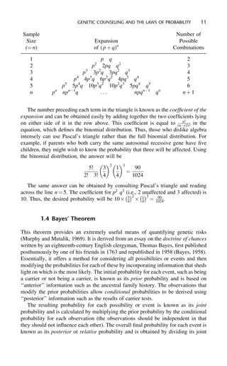
SlideShare a Scribd company logo
1 of 4
Download to read offline
GENETIC COUNSELING AND THE LAWS OF PROBABILITY             11

 Sample                                                 Number of
   Size                    Expansion                     Possible
  (¼ n)                    of ( p þ q)n                Combinations
___________________________________________________________________
    1                         p q                           2
    2                     p2 2pq q2                         3
    3                 p3 3p2q 3pq2 q3                       4
    4              p4 4p3q 6p2q2 4pq3 q4                    5
    5          p5 5p4q 10p3q2 10p2q3 5pq4 q5                6
    n      pn npnÀ1q          ...        npqnÀ1 qn        nþ1


   The number preceding each term in the triangle is known as the coefficient of the
expansion and can be obtained easily by adding together the two coefficients lying
                                                                          n!
on either side of it in the row above. This coefficient is equal to (nÀr)!r! in the
equation, which defines the binomial distribution. Thus, those who dislike algebra
intensely can use Pascal’s triangle rather than the full binomial distribution. For
example, if parents who both carry the same autosomal recessive gene have five
children, they might wish to know the probability that three will be affected. Using
the binomial distribution, the answer will be
                                    2  3
                               5!    3     1       90
                                               ¼
                             2! 3! 4       4      1024
   The same answer can be obtained by consulting Pascal’s triangle and reading
across the line n ¼ 5. The coefficient for p2 q3 À Á 2À unaffected and 3 affected) is
                                                (i.e., Á
                                                   2     3
10. Thus, the desired probability will be 10Â 3 Â 1 ¼ 1024.
                                                 4     4
                                                              90


         1.4 Bayes’ Theorem

This theorem provides an extremely useful means of quantifying genetic risks
(Murphy and Mutalik, 1969). It is derived from an essay on the doctrine of chances
written by an eighteenth-century English clergyman, Thomas Bayes, first published
posthumously by one of his friends in 1763 and republished in 1958 (Bayes, 1958).
Essentially, it offers a method for considering all possibilities or events and then
modifying the probabilities for each of these by incorporating information that sheds
light on which is the most likely. The initial probability for each event, such as being
a carrier or not being a carrier, is known as its prior probability and is based on
‘‘anterior’’ information such as the ancestral family history. The observations that
modify the prior probabilities allow conditional probabilities to be derived using
‘‘posterior’’ information such as the results of carrier tests.
   The resulting probability for each possibility or event is known as its joint
probability and is calculated by multiplying the prior probability by the conditional
probability for each observation (the observations should be independent in that
they should not influence each other). The overall final probability for each event is
known as its posterior or relative probability and is obtained by dividing its joint
12       INTRODUCTION TO RISK CALCULATION IN GENETIC COUNSELING

probability by the sum of all of the joint probabilities. This has the effect of ensuring
that the sum of all of the posterior probabilities always equals 1. Alternatively,
posterior probabilities can be expressed in the form of odds for or against a particular
event occurring or not occurring.
   On first reading this can be very confusing, and the reader will not necessarily be
helped by the following formal statement of Bayes’ theorem:
     1. If the prior probability of an event C occurring is denoted as P(C) and
     2. the prior probability of event C not occurring is denoted as P(NC) and
     3. the conditional probability of observation O occurring if C occurs equals
        P(OjC ) and
     4. the conditional probability of observation O occurring if C does not occur equals
        P(OjNC ), then the overall probability of event C given that O is observed equals

                               P(C ) multiplied by P (OjC )
             [P(C ) multiplied by P(OjC )] þ [P(NC) multiplied by P(OjNC )]

        This may be a little clearer if a Bayesian table (Table 1.1) is constructed.
        The posterior probability of event C occurring equals

                                      P(C ) Â P (OjC )
                          [P(C ) Â P(OjC )] þ [P(NC ) Â P(OjNC )]

        The posterior probability of event C not occurring equals

                                     P(NC ) Â P(OjNC )
                          [P(C ) Â P(OjC )] þ [P(NC ) Â P(OjNC )]

        This is not nearly as complicated or difficult as it seems. If you are not
        convinced, then consider the following example.


           Example 6
A woman, II2 in Figure 1.1, wishes to know the probability that she is a carrier
of Duchenne muscular dystrophy. Her concern is based upon her family history,
which reveals an affected brother and an affected maternal uncle. This is anterior
information that enables the prior probability that she is a carrier P(C) to be de-


           Table 1.1.
                                    Event C                      Event C Does
           Probability              Occurs                       Not Occur

           Prior                    P(C )                        P(NC )
           Conditional              P(OjC )                      P(OjNC )
             O occurs
                                    ____________                 _______________
           Joint                    P(C ) Â P(OjC )              P(NC ) Â P(OjNC )
GENETIC COUNSELING AND THE LAWS OF PROBABILITY                     13


Figure 1.1. When calculating the
probability that II2 is a carrier of
Duchenne muscular dystrophy Bayes’
theorem provides a method for taking
into account the fact that she already
has three unaffected sons.


termined. As her mother (I2) must be a carrier, there is a prior probability of 1/2 that
II2 is a carrier and an equal prior probability of 1/2 that she is not a carrier.
   Posterior information is provided by the fact that the consultand already has three
unaffected sons. If the consultand is a carrier, then each of her sons will have a risk of
1 in 2 of being affected. Thus, P(OjC ) equals 1 ⁄ 2 Â 1 ⁄ 2Â 1 ⁄ 2 since the consultand
has three unaffected sons, and P(OjNC ) equals 1 Â 1 Â 1, since if the consultand is
not a carrier, there is a probability of 1 (1 À m, to be exact, but m—the mutation rate—
can be ignored since it is less than 1/1000) that a son will be unaffected.
   This information is used to construct a Bayesian table (Table 1.2). The pos-
terior probability that the consultand is a carrier equals 1 ⁄ 16 ⁄ (1 ⁄ 16 þ 1 ⁄ 2), which
equals 1/9. Alternatively, the posterior probability can be stated in the form of odds
by indicating that there are 8 chances to 1 that the consultand is not a carrier.
   Effectively, in this example Bayes’ theorem has been used to quantify the in-
tuitive recognition that the birth of three unaffected sons makes it rather unlikely


             Table 1.2.
                                               Consultand Is                     Consultand Is
             Probability                         a Carrier                       Not a Carrier

             Prior                                   1                                  1
                                                     2                                  2
             Conditional
                                                     1
             3 unaffected sons                                                        1
                                                     8
                                                   _____                            _____
                                                     1                                1
             Joint
                                                    16                                2
             Odds                                     1            to                   8
                                                                    1
                                                                           1
             Posterior probability that consultand is a carrier ¼ 116
                                                                       1 ¼
                                                                  16 Â 2   9
                                                                             1
                                                                                        8
             Posterior probability that consultand is not a carrier ¼        2
                                                                                    ¼
                                                                        1
                                                                        16   Â1
                                                                              2         9
14       INTRODUCTION TO RISK CALCULATION IN GENETIC COUNSELING

that the consultand is a carrier. The greater the number of unaffected sons, then, the
more likely it becomes that the consultand is not a carrier. Obviously, the birth of
one affected son would totally negate the conditional probability contributed by
unaffected sons by introducing conditional probabilities of 1/2 (carrier) versus m
(new mutation) in the noncarrier column. In other words, the birth of an affected
son would make it overwhelmingly likely that the consultand is a carrier.


     Key Point 4

     Bayes’ theorem provides a method for taking into account all relevant information
     when calculating the probability of an event such as carrier status. Key points to
     remember are:

     1. A table should be drawn up that includes all relevant possibilities.
     2. The prior probability for each possibility is derived from ancestral anterior in-
        formation.
     3. The conditional probabilities are obtained from posterior information that
        sheds light on which initial possibility is more or less likely. Conditional prob-
        abilities can be calculated by asking ‘‘What is the probability that this observation
        would be made given that the initial possibility or event occurs or applies?’’
     4. The joint probability for each possibility is calculated and then compared with
        the other joint probabilities to give a posterior or relative probability for each
        possibility or event.
     5. All relevant information should be used once and only once.


    The concepts introduced in this chapter, and in Bayes’ theorem in particular,
are not easy to grasp. However, with a little practice, even the most reluctant
mathematician can become reasonably proficient at simple probability calculations.
More testing examples are provided in the next four chapters. Readers who are
still struggling with the underlying principles are invited to consult the review by
Ogino and Wilson (2004), which provides a very clear explanation of how to apply
Bayesian analysis.


           1.5 Case Scenario

A woman, II2 in Figure 1.2, is referred from the antenatal clinic for genetic risk
assessment. She is 20 weeks pregnant and is known to have two maternal uncles and a
brother with severe learning disability. Investigations undertaken in the past, including
Fragile X mutation analysis, have failed to identify a specific cause, prompting a
clinical diagnosis of nonspecific X-linked mental retardation. Ultrasonography has
revealed that this woman is carrying male twins (III2 and III3) of unknown zygosity.
The woman specifically wishes to know the probability that one or both of her unborn
sons will be affected.

More Related Content

Similar to Young P11 14

A Note on the Asymptotic Convergence of Bernoulli Distribution
A Note on the Asymptotic Convergence of Bernoulli DistributionA Note on the Asymptotic Convergence of Bernoulli Distribution
A Note on the Asymptotic Convergence of Bernoulli DistributionBRNSS Publication Hub
 
PG STAT 531 Lecture 5 Probability Distribution
PG STAT 531 Lecture 5 Probability DistributionPG STAT 531 Lecture 5 Probability Distribution
PG STAT 531 Lecture 5 Probability DistributionAashish Patel
 
A Measure Of Independence For A Multifariate Normal Distribution And Some Con...
A Measure Of Independence For A Multifariate Normal Distribution And Some Con...A Measure Of Independence For A Multifariate Normal Distribution And Some Con...
A Measure Of Independence For A Multifariate Normal Distribution And Some Con...ganuraga
 
A Measure Of Independence For A Multifariate Normal Distribution And Some Con...
A Measure Of Independence For A Multifariate Normal Distribution And Some Con...A Measure Of Independence For A Multifariate Normal Distribution And Some Con...
A Measure Of Independence For A Multifariate Normal Distribution And Some Con...gueste63bd9
 
2 Review of Statistics. 2 Review of Statistics.
2 Review of Statistics. 2 Review of Statistics.2 Review of Statistics. 2 Review of Statistics.
2 Review of Statistics. 2 Review of Statistics.WeihanKhor2
 

Similar to Young P11 14 (7)

01_AJMS_158_18_RA.pdf
01_AJMS_158_18_RA.pdf01_AJMS_158_18_RA.pdf
01_AJMS_158_18_RA.pdf
 
01_AJMS_158_18_RA.pdf
01_AJMS_158_18_RA.pdf01_AJMS_158_18_RA.pdf
01_AJMS_158_18_RA.pdf
 
A Note on the Asymptotic Convergence of Bernoulli Distribution
A Note on the Asymptotic Convergence of Bernoulli DistributionA Note on the Asymptotic Convergence of Bernoulli Distribution
A Note on the Asymptotic Convergence of Bernoulli Distribution
 
PG STAT 531 Lecture 5 Probability Distribution
PG STAT 531 Lecture 5 Probability DistributionPG STAT 531 Lecture 5 Probability Distribution
PG STAT 531 Lecture 5 Probability Distribution
 
A Measure Of Independence For A Multifariate Normal Distribution And Some Con...
A Measure Of Independence For A Multifariate Normal Distribution And Some Con...A Measure Of Independence For A Multifariate Normal Distribution And Some Con...
A Measure Of Independence For A Multifariate Normal Distribution And Some Con...
 
A Measure Of Independence For A Multifariate Normal Distribution And Some Con...
A Measure Of Independence For A Multifariate Normal Distribution And Some Con...A Measure Of Independence For A Multifariate Normal Distribution And Some Con...
A Measure Of Independence For A Multifariate Normal Distribution And Some Con...
 
2 Review of Statistics. 2 Review of Statistics.
2 Review of Statistics. 2 Review of Statistics.2 Review of Statistics. 2 Review of Statistics.
2 Review of Statistics. 2 Review of Statistics.
 

Young P11 14

  • 1. GENETIC COUNSELING AND THE LAWS OF PROBABILITY 11 Sample Number of Size Expansion Possible (¼ n) of ( p þ q)n Combinations ___________________________________________________________________ 1 p q 2 2 p2 2pq q2 3 3 p3 3p2q 3pq2 q3 4 4 p4 4p3q 6p2q2 4pq3 q4 5 5 p5 5p4q 10p3q2 10p2q3 5pq4 q5 6 n pn npnÀ1q ... npqnÀ1 qn nþ1 The number preceding each term in the triangle is known as the coefficient of the expansion and can be obtained easily by adding together the two coefficients lying n! on either side of it in the row above. This coefficient is equal to (nÀr)!r! in the equation, which defines the binomial distribution. Thus, those who dislike algebra intensely can use Pascal’s triangle rather than the full binomial distribution. For example, if parents who both carry the same autosomal recessive gene have five children, they might wish to know the probability that three will be affected. Using the binomial distribution, the answer will be 2 3 5! 3 1 90 ¼ 2! 3! 4 4 1024 The same answer can be obtained by consulting Pascal’s triangle and reading across the line n ¼ 5. The coefficient for p2 q3 À Á 2À unaffected and 3 affected) is (i.e., Á 2 3 10. Thus, the desired probability will be 10Â 3 Â 1 ¼ 1024. 4 4 90 1.4 Bayes’ Theorem This theorem provides an extremely useful means of quantifying genetic risks (Murphy and Mutalik, 1969). It is derived from an essay on the doctrine of chances written by an eighteenth-century English clergyman, Thomas Bayes, first published posthumously by one of his friends in 1763 and republished in 1958 (Bayes, 1958). Essentially, it offers a method for considering all possibilities or events and then modifying the probabilities for each of these by incorporating information that sheds light on which is the most likely. The initial probability for each event, such as being a carrier or not being a carrier, is known as its prior probability and is based on ‘‘anterior’’ information such as the ancestral family history. The observations that modify the prior probabilities allow conditional probabilities to be derived using ‘‘posterior’’ information such as the results of carrier tests. The resulting probability for each possibility or event is known as its joint probability and is calculated by multiplying the prior probability by the conditional probability for each observation (the observations should be independent in that they should not influence each other). The overall final probability for each event is known as its posterior or relative probability and is obtained by dividing its joint
  • 2. 12 INTRODUCTION TO RISK CALCULATION IN GENETIC COUNSELING probability by the sum of all of the joint probabilities. This has the effect of ensuring that the sum of all of the posterior probabilities always equals 1. Alternatively, posterior probabilities can be expressed in the form of odds for or against a particular event occurring or not occurring. On first reading this can be very confusing, and the reader will not necessarily be helped by the following formal statement of Bayes’ theorem: 1. If the prior probability of an event C occurring is denoted as P(C) and 2. the prior probability of event C not occurring is denoted as P(NC) and 3. the conditional probability of observation O occurring if C occurs equals P(OjC ) and 4. the conditional probability of observation O occurring if C does not occur equals P(OjNC ), then the overall probability of event C given that O is observed equals P(C ) multiplied by P (OjC ) [P(C ) multiplied by P(OjC )] þ [P(NC) multiplied by P(OjNC )] This may be a little clearer if a Bayesian table (Table 1.1) is constructed. The posterior probability of event C occurring equals P(C ) Â P (OjC ) [P(C ) Â P(OjC )] þ [P(NC ) Â P(OjNC )] The posterior probability of event C not occurring equals P(NC ) Â P(OjNC ) [P(C ) Â P(OjC )] þ [P(NC ) Â P(OjNC )] This is not nearly as complicated or difficult as it seems. If you are not convinced, then consider the following example. Example 6 A woman, II2 in Figure 1.1, wishes to know the probability that she is a carrier of Duchenne muscular dystrophy. Her concern is based upon her family history, which reveals an affected brother and an affected maternal uncle. This is anterior information that enables the prior probability that she is a carrier P(C) to be de- Table 1.1. Event C Event C Does Probability Occurs Not Occur Prior P(C ) P(NC ) Conditional P(OjC ) P(OjNC ) O occurs ____________ _______________ Joint P(C ) Â P(OjC ) P(NC ) Â P(OjNC )
  • 3. GENETIC COUNSELING AND THE LAWS OF PROBABILITY 13 Figure 1.1. When calculating the probability that II2 is a carrier of Duchenne muscular dystrophy Bayes’ theorem provides a method for taking into account the fact that she already has three unaffected sons. termined. As her mother (I2) must be a carrier, there is a prior probability of 1/2 that II2 is a carrier and an equal prior probability of 1/2 that she is not a carrier. Posterior information is provided by the fact that the consultand already has three unaffected sons. If the consultand is a carrier, then each of her sons will have a risk of 1 in 2 of being affected. Thus, P(OjC ) equals 1 ⁄ 2 Â 1 ⁄ 2Â 1 ⁄ 2 since the consultand has three unaffected sons, and P(OjNC ) equals 1 Â 1 Â 1, since if the consultand is not a carrier, there is a probability of 1 (1 À m, to be exact, but m—the mutation rate— can be ignored since it is less than 1/1000) that a son will be unaffected. This information is used to construct a Bayesian table (Table 1.2). The pos- terior probability that the consultand is a carrier equals 1 ⁄ 16 ⁄ (1 ⁄ 16 þ 1 ⁄ 2), which equals 1/9. Alternatively, the posterior probability can be stated in the form of odds by indicating that there are 8 chances to 1 that the consultand is not a carrier. Effectively, in this example Bayes’ theorem has been used to quantify the in- tuitive recognition that the birth of three unaffected sons makes it rather unlikely Table 1.2. Consultand Is Consultand Is Probability a Carrier Not a Carrier Prior 1 1 2 2 Conditional 1 3 unaffected sons 1 8 _____ _____ 1 1 Joint 16 2 Odds 1 to 8 1 1 Posterior probability that consultand is a carrier ¼ 116 1 ¼ 16 Â 2 9 1 8 Posterior probability that consultand is not a carrier ¼ 2 ¼ 1 16 Â1 2 9
  • 4. 14 INTRODUCTION TO RISK CALCULATION IN GENETIC COUNSELING that the consultand is a carrier. The greater the number of unaffected sons, then, the more likely it becomes that the consultand is not a carrier. Obviously, the birth of one affected son would totally negate the conditional probability contributed by unaffected sons by introducing conditional probabilities of 1/2 (carrier) versus m (new mutation) in the noncarrier column. In other words, the birth of an affected son would make it overwhelmingly likely that the consultand is a carrier. Key Point 4 Bayes’ theorem provides a method for taking into account all relevant information when calculating the probability of an event such as carrier status. Key points to remember are: 1. A table should be drawn up that includes all relevant possibilities. 2. The prior probability for each possibility is derived from ancestral anterior in- formation. 3. The conditional probabilities are obtained from posterior information that sheds light on which initial possibility is more or less likely. Conditional prob- abilities can be calculated by asking ‘‘What is the probability that this observation would be made given that the initial possibility or event occurs or applies?’’ 4. The joint probability for each possibility is calculated and then compared with the other joint probabilities to give a posterior or relative probability for each possibility or event. 5. All relevant information should be used once and only once. The concepts introduced in this chapter, and in Bayes’ theorem in particular, are not easy to grasp. However, with a little practice, even the most reluctant mathematician can become reasonably proficient at simple probability calculations. More testing examples are provided in the next four chapters. Readers who are still struggling with the underlying principles are invited to consult the review by Ogino and Wilson (2004), which provides a very clear explanation of how to apply Bayesian analysis. 1.5 Case Scenario A woman, II2 in Figure 1.2, is referred from the antenatal clinic for genetic risk assessment. She is 20 weeks pregnant and is known to have two maternal uncles and a brother with severe learning disability. Investigations undertaken in the past, including Fragile X mutation analysis, have failed to identify a specific cause, prompting a clinical diagnosis of nonspecific X-linked mental retardation. Ultrasonography has revealed that this woman is carrying male twins (III2 and III3) of unknown zygosity. The woman specifically wishes to know the probability that one or both of her unborn sons will be affected.