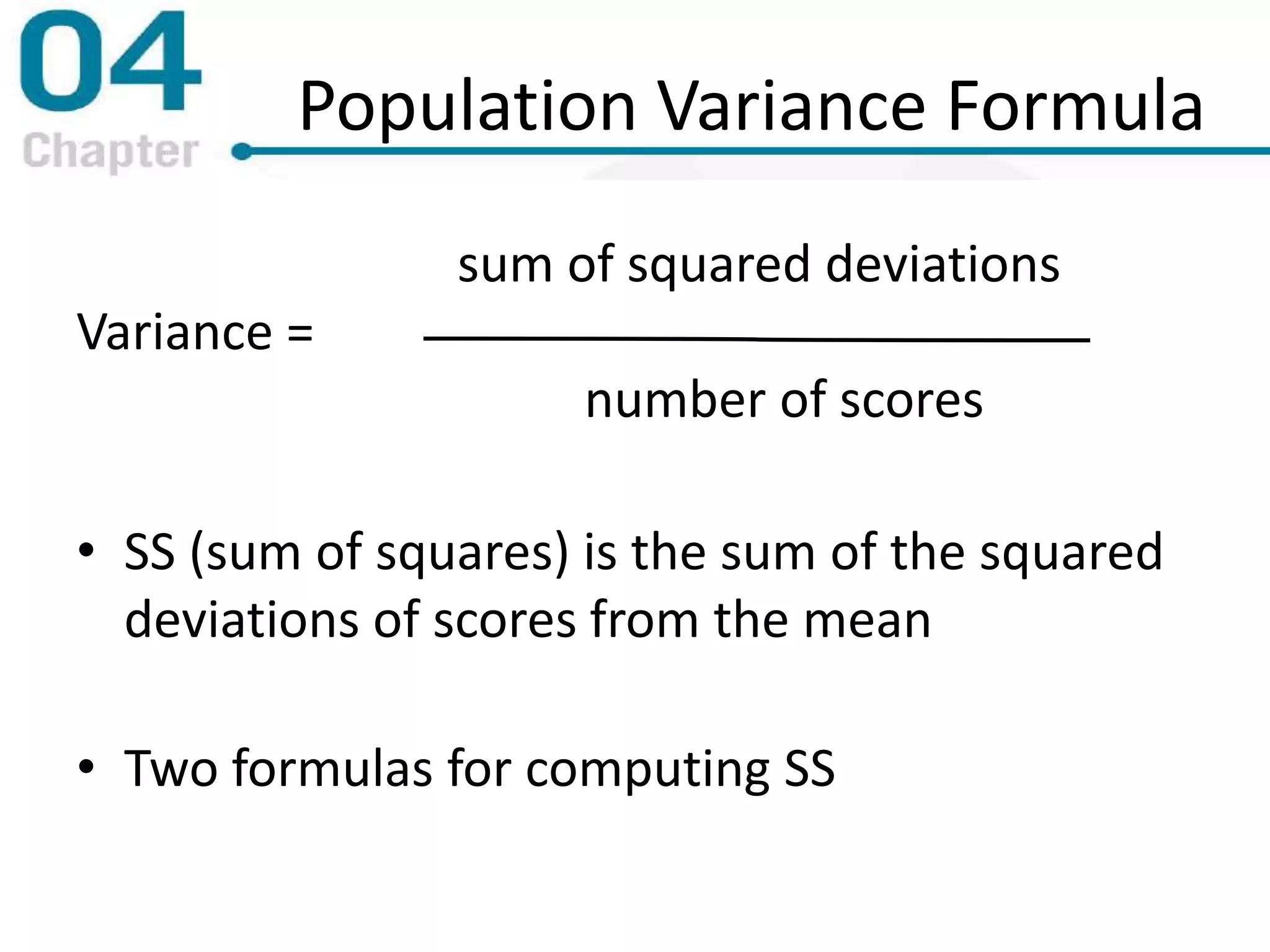
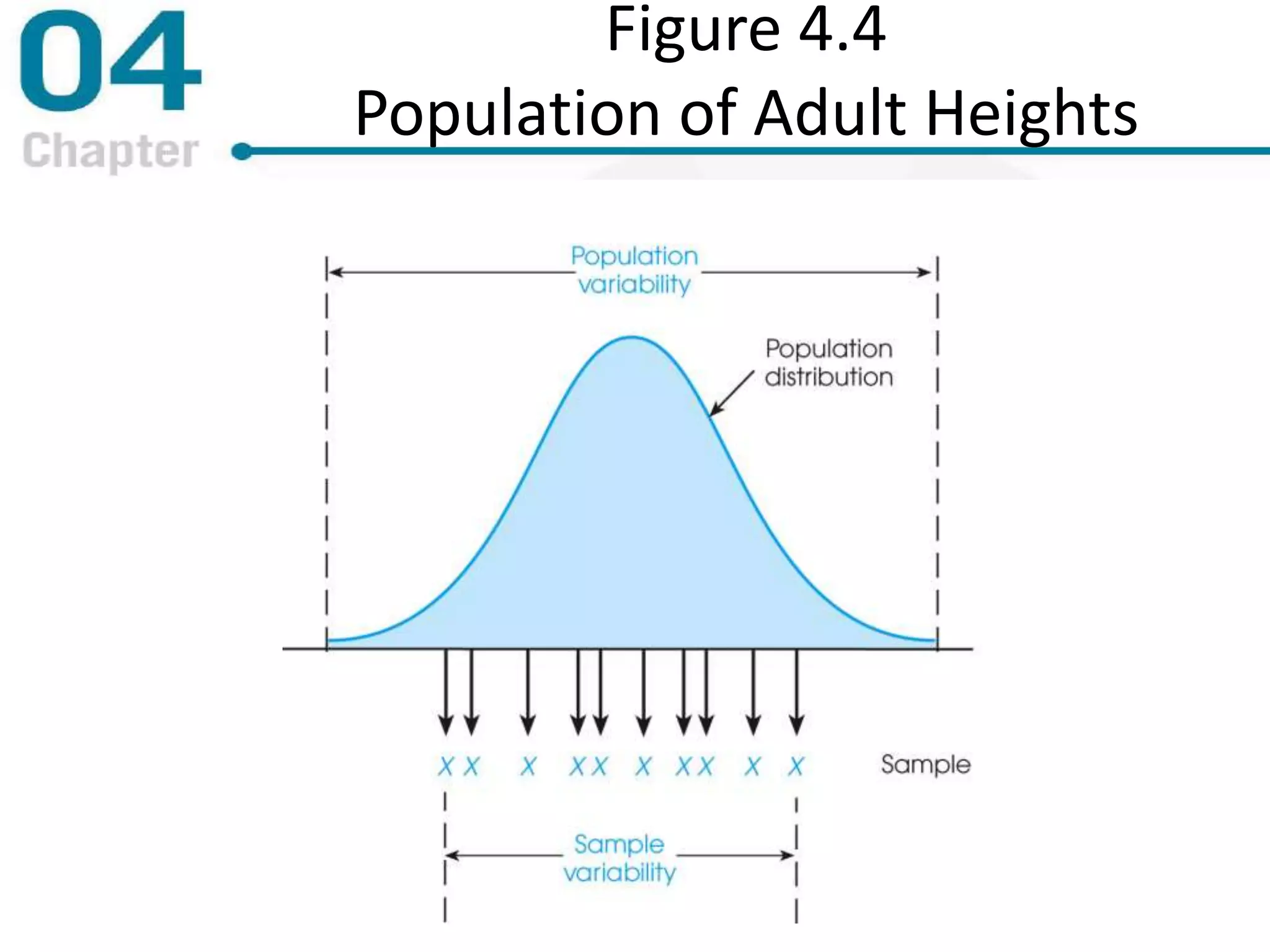
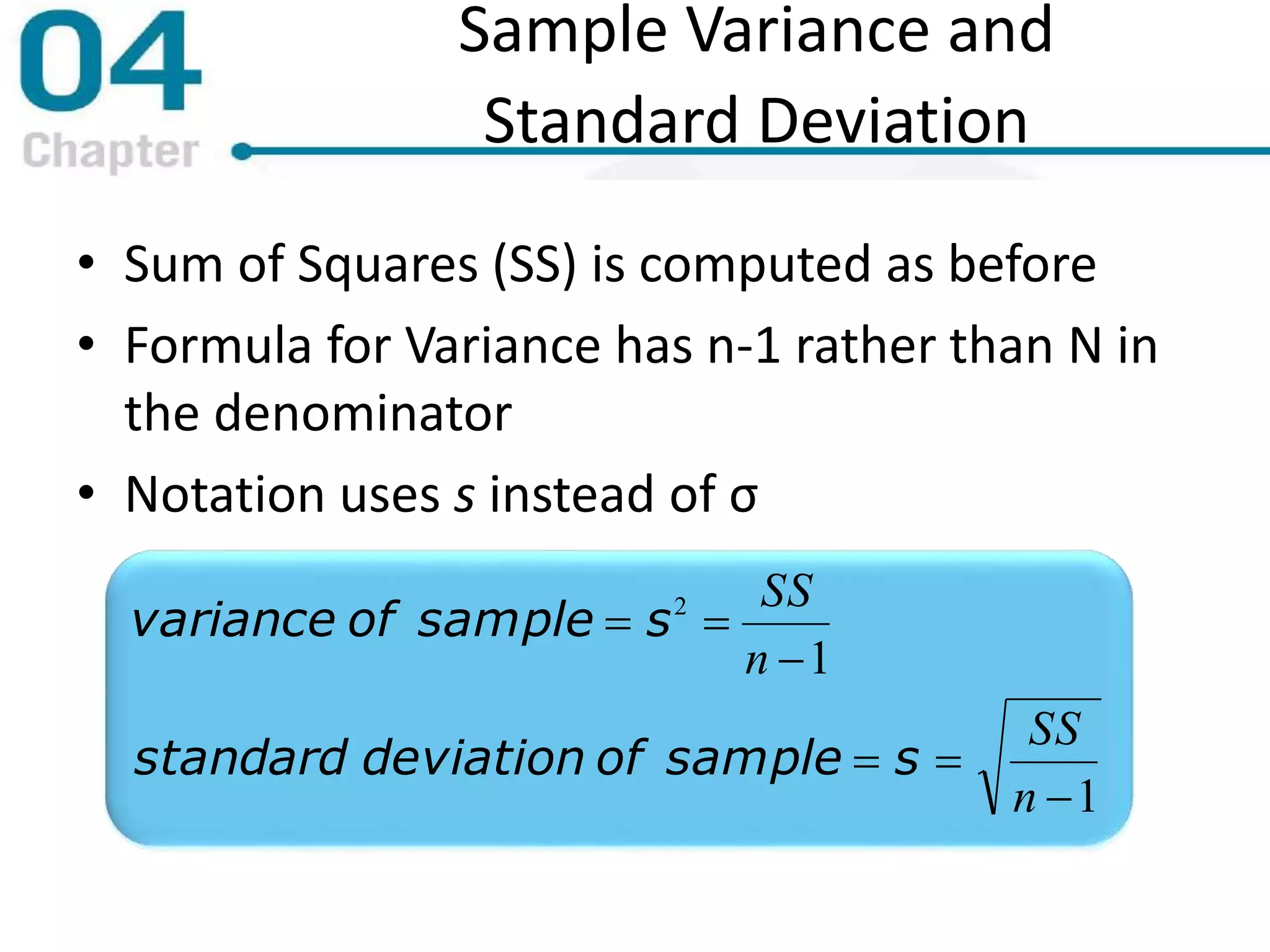
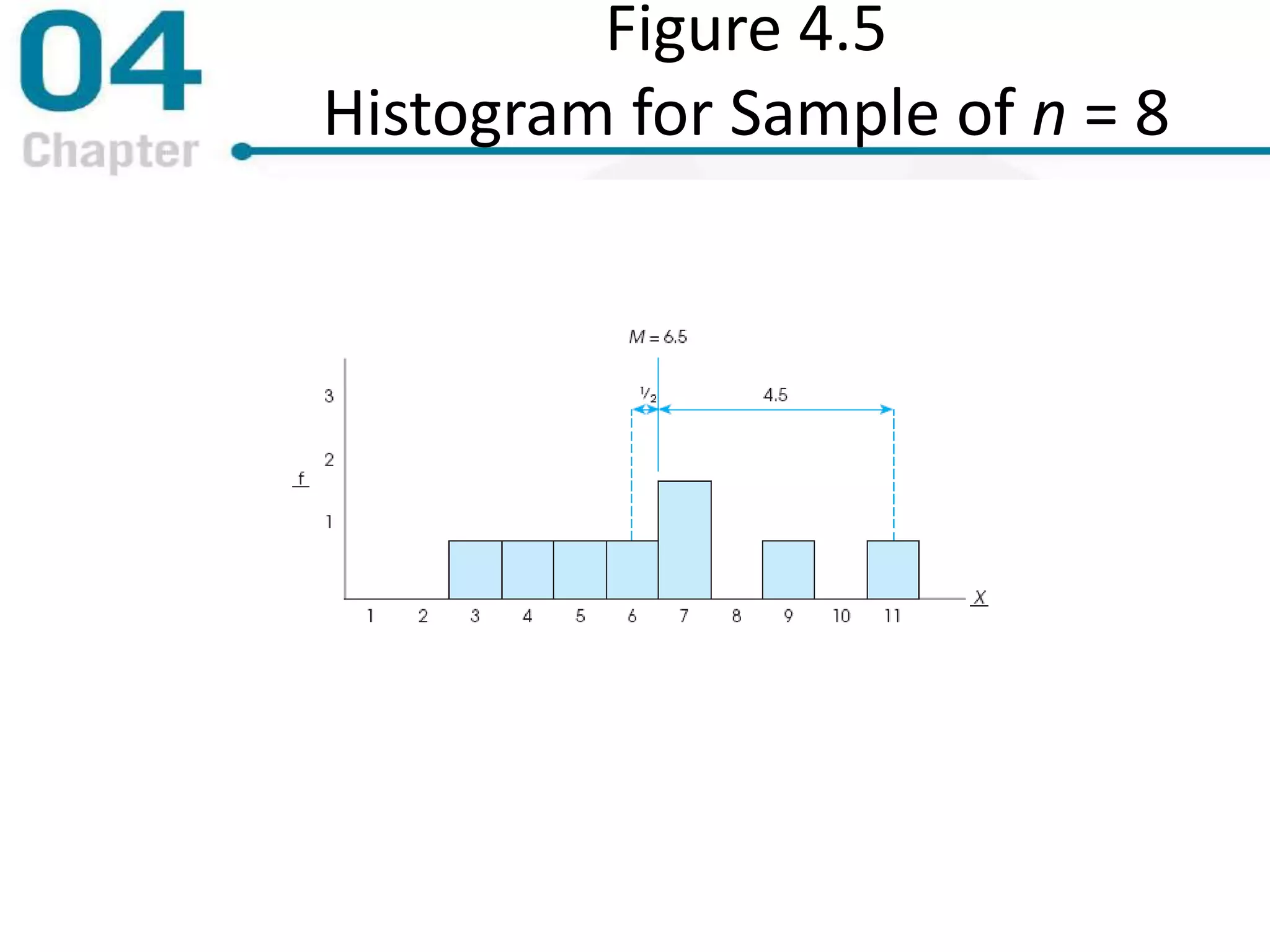
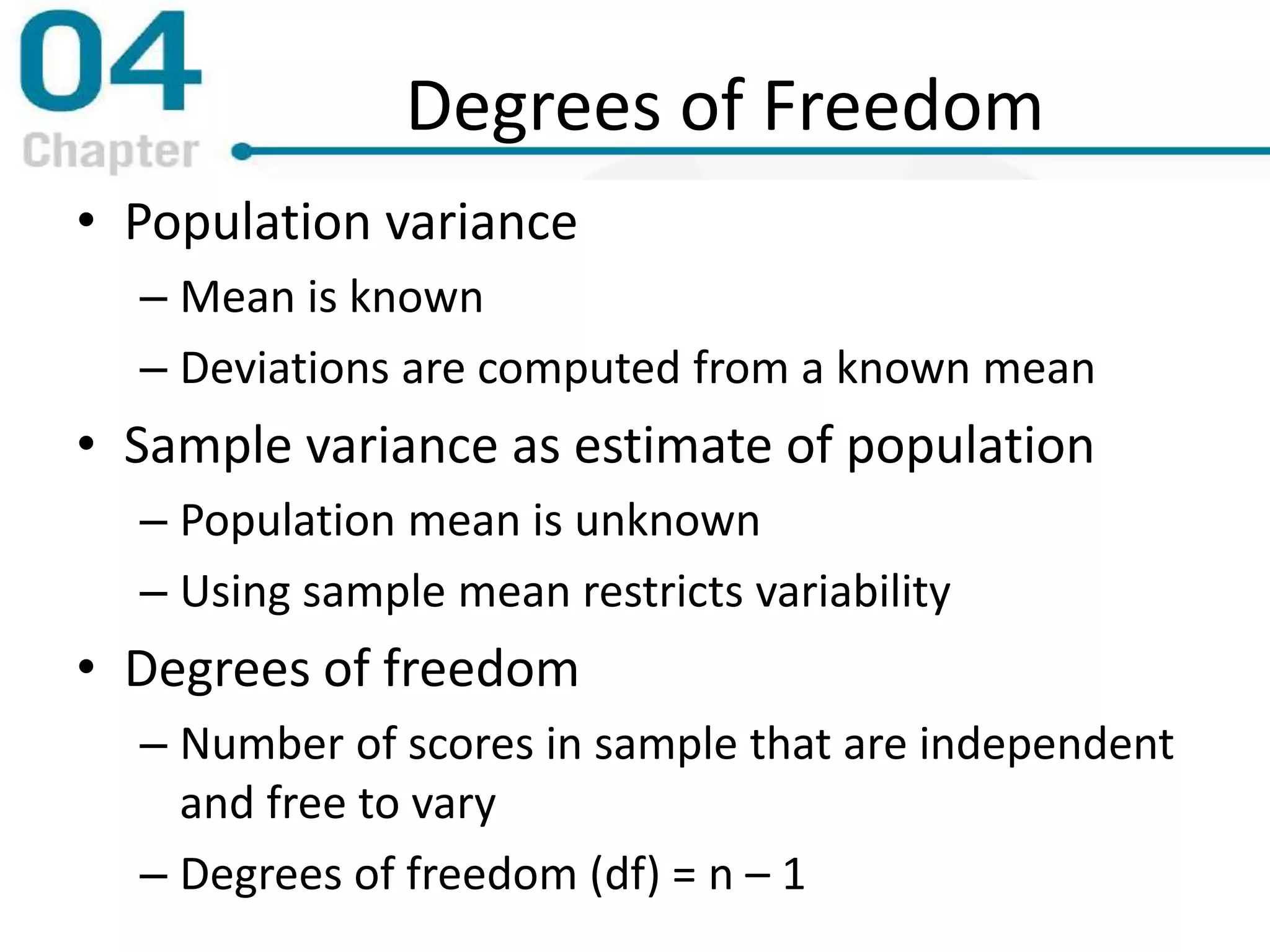
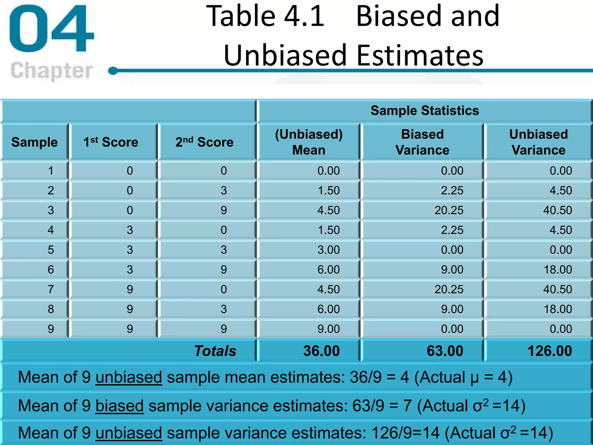
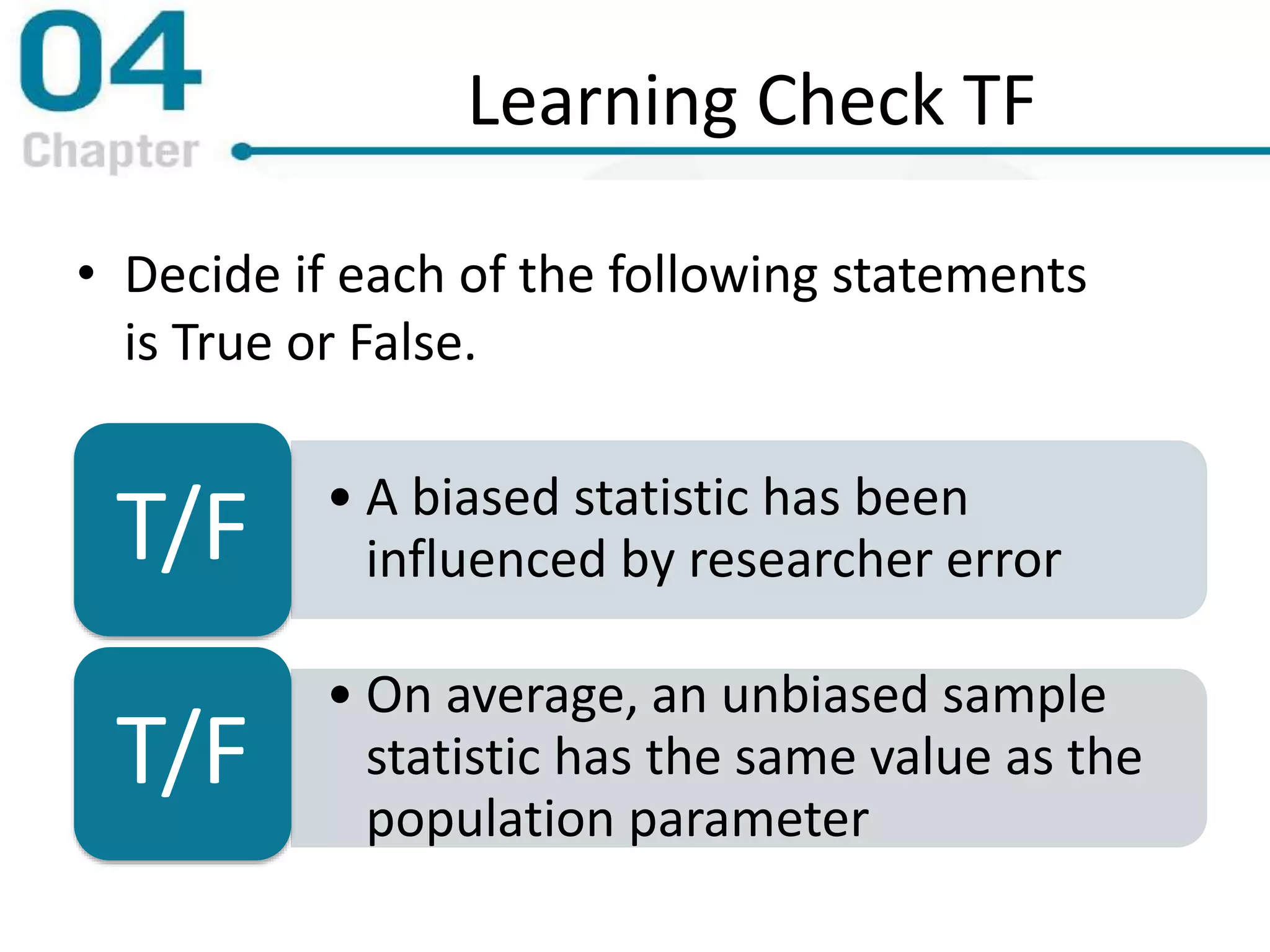
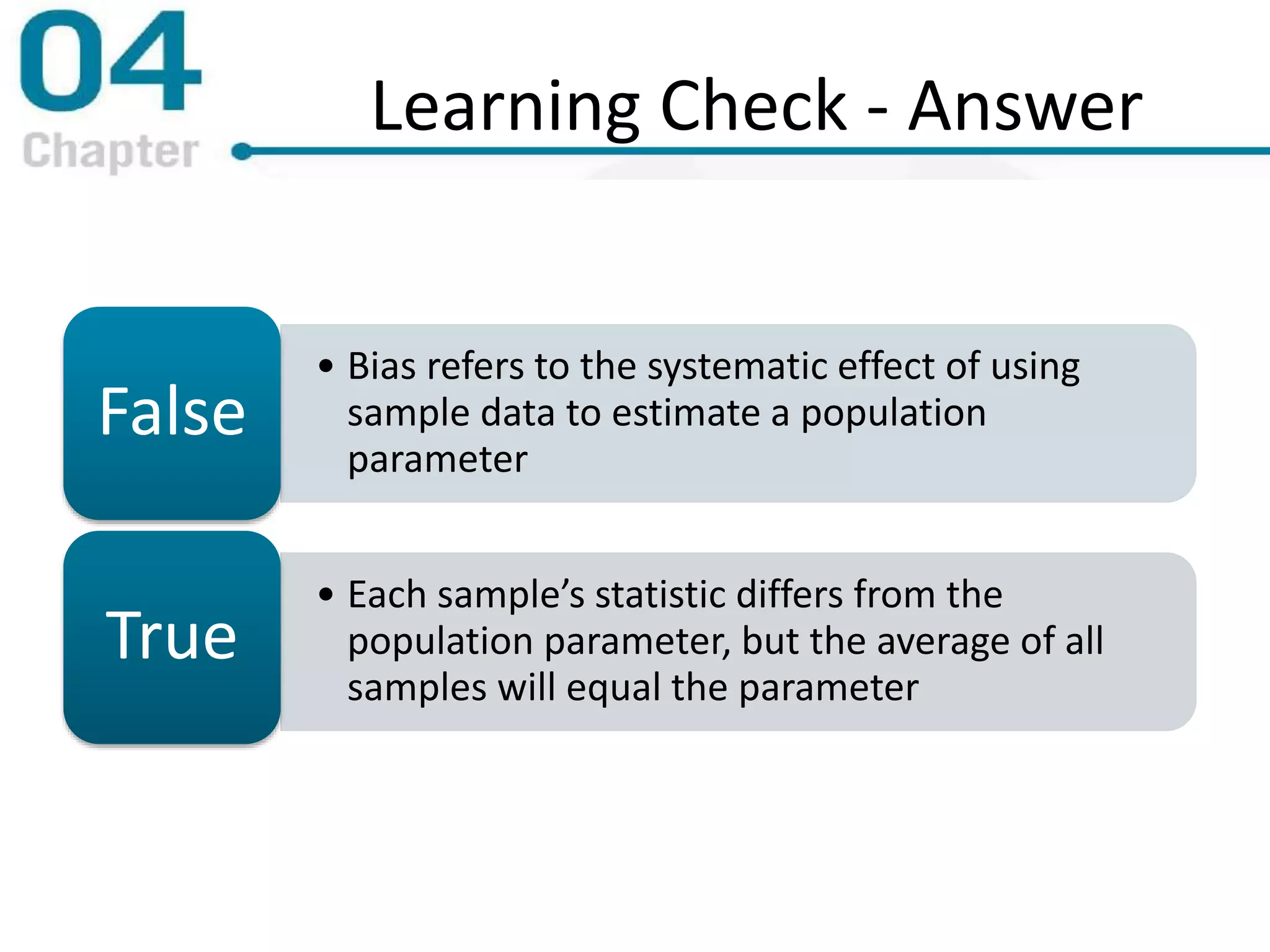
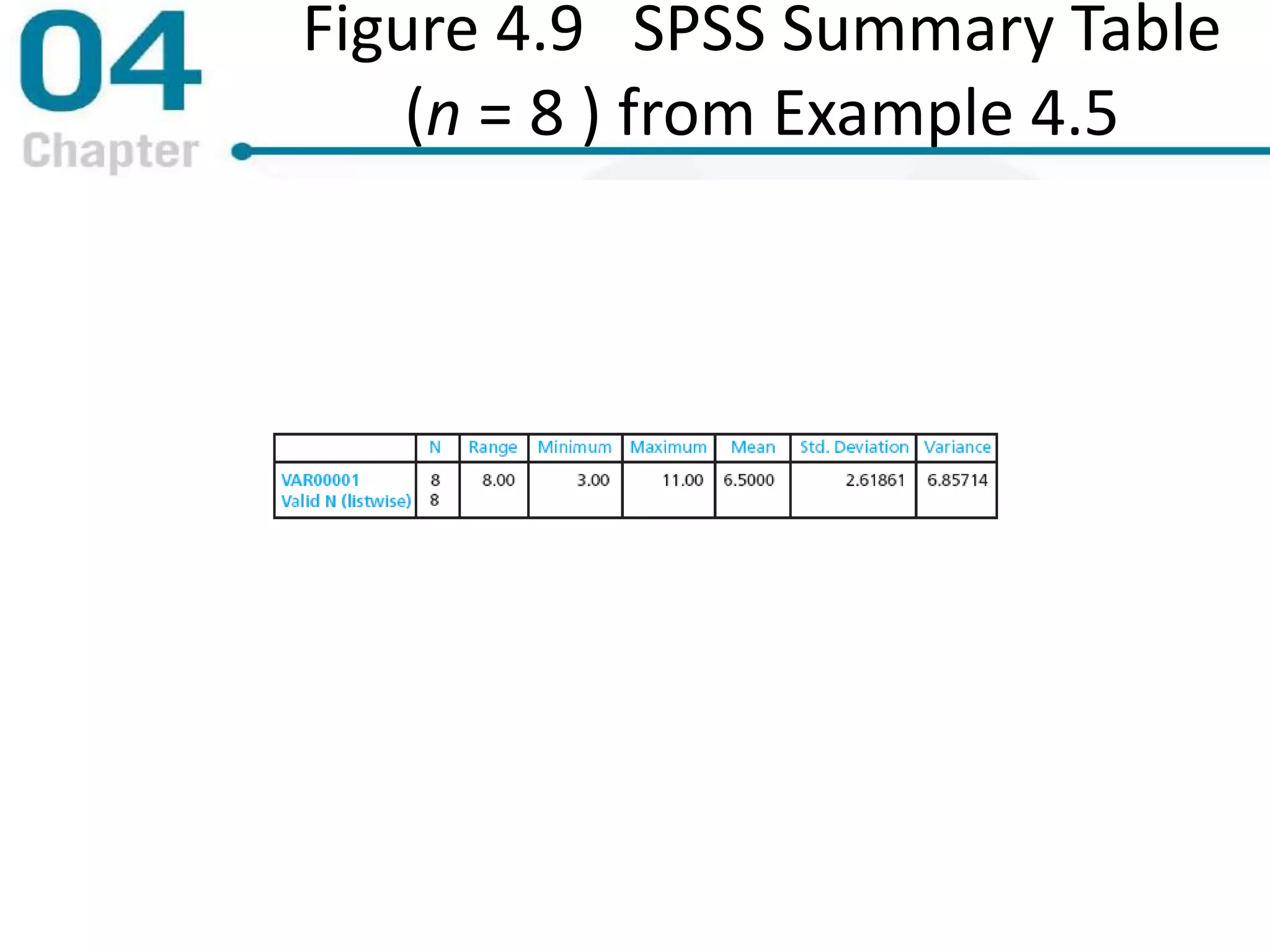
Chapter 4
Measures of Variability
PowerPoint Lecture Slides
Essentials of Statistics for the
Behavioral Sciences
Eighth Edition
by Frederick J Gravetter and Larry B. Wallnau
Learning Outcomes
• Understand purpose of measuring variability1
• Define range2
• Compute range3
• Understand variance and standard deviation4
• Calculate SS, variance, standard deviation of population5
• Calculate SS, variance, standard deviation of sample6
Tools You Will Need
• Summation notation (Chapter 1)
• Central tendency (Chapter 3)
– Mean
– Median
4.1 Overview
• Variability can be defined several ways
– A quantitative distance measure based on the
differences between scores
– Describes distance of the spread of scores or
distance of a score from the mean
• Purposes of Measure of Variability
– Describe the distribution
– Measure how well an individual score represents
the distribution
Figure 4.1
Population Distributions
Three Measures of Variability
• The Range
• The Variance
• The Standard Deviation
• The distance covered by the scores in a
distribution
– From smallest value to highest value
• For continuous data, real limits are used
• Based on two scores, not all the data
– An imprecise, unreliable measure of variability
range = URL for Xmax — LRL for Xmin
4.2 The Range
4.3 Standard Deviation and
Variance for a Population
• Most common and most important measure
of variability is the standard deviation
– A measure of the standard, or average, distance
from the mean
– Describes whether the scores are clustered closely
around the mean or are widely scattered
• Calculation differs for population and samples
• Variance is a necessary companion concept to
standard deviation but not the same concept
Defining the Standard Deviation
• Step One: Determine the Deviation
• Deviation is distance from the mean
• Step Two: Find a “sum of deviations” to use as
a basis of finding an “average deviation”
– Two problems
• Deviations sum to 0 (because M is balance point)
• If sum always 0, “Mean Deviation” will always be 0.
– Need a new strategy!
Deviation score = X — μ
Defining the Standard Deviation
(continued)
• Step Two Revised: Remove negative deviations
– First square each deviation score
– Then sum the Squared Deviations (SS)
• Step Three: Average the squared deviations
– Mean Squared Deviation is known as “Variance”
– Variability is now measured in squared units
Population variance equals mean (average)
squared deviation (distance) of the scores
from the population mean
Defining the Standard Deviation
(continued)
• Step Four:
– Goal: to compute a measure of the “standard”
(average) distance of the scores from the mean
– Variance measures the average squared distance
from the mean—not quite our goal
• Adjust for having squared all the differences
by taking the square root of the variance
• Standard Deviation = Variance
Figure 4.2
Figure 4.3
Population Variance Formula
sum of squared deviations
Variance =
number of scores
• SS (sum of squares) is the sum of the squared
deviations of scores from the mean
• Two formulas for computing SS
Two formulas for SS
Definitional Formula
• Find each deviation score
(X–μ)
• Square each deviation
score, (X–μ)2
• Sum up the squared
deviations
Computational Formula
 2
  XSS
 
 
N
X
XSS
2
2
• Square each score and sum
the squared scores
• Find the sum of scores,
square it, divide by N
• Subtract the second part
from the first
Caution Required!
When using the computational formula, remember…
  22
)( XX
 2
XSS
 2
)( XSS
Population Variance:
Formula and Notation
Formula
N
SS
N
SS
deviationstandard
variance


Notation
• Variance is the average of
squared deviations, so we
identify population variance
with a lowercase Greek
letter sigma squared: σ2
• Standard deviation is the
square root of the variance,
so we identify it with a
lowercase Greek letter
sigma: σ
Learning Check
• Decide if each of the following statements
is True or False.
• The computational & definitional
formulas for SS sometimes give
different results
T/F
• If all the scores in a data set are
the same, the Standard Deviation
is equal to 1.00
T/F
Learning Check - Answer
• The computational formula is just an algebraic
rearrangement of the definitional formula.
Results are identical
False
• When all the scores are the same, they are all
equal to the mean. Their deviations = 0, as
does their Standard Deviation
False
Learning Check
• The standard deviation measures …
• Sum of squared deviation scoresA
• Standard distance of a score from the meanB
• Average deviation of a score from the meanC
• Average squared distance of a score from the meanD
Learning Check - Answer
• The standard deviation measures …
• Sum of squared deviation scoresA
• Standard distance of a score from the meanB
• Average deviation of a score from the meanC
• Average squared distance of a score from the meanD
4.4 Standard Deviation and
Variance for a Sample
• Goal of inferential statistics:
– Draw general conclusions about population
– Based on limited information from a sample
• Samples differ from the population
– Samples have less variability
– Computing the Variance and Standard Deviation in
the same way as for a population would give a
biased estimate of the population values
Figure 4.4
Population of Adult Heights
Sample Variance and
Standard Deviation
• Sum of Squares (SS) is computed as before
• Formula for Variance has n-1 rather than N in
the denominator
• Notation uses s instead of σ
1
1
2




n
SS
n
SS
ssampleofdeviationstandard
ssampleofvariance
Figure 4.5
Histogram for Sample of n = 8
Degrees of Freedom
• Population variance
– Mean is known
– Deviations are computed from a known mean
• Sample variance as estimate of population
– Population mean is unknown
– Using sample mean restricts variability
• Degrees of freedom
– Number of scores in sample that are independent
and free to vary
– Degrees of freedom (df) = n – 1
Learning Check
• A sample of four scores has SS = 24.
What is the variance?
• The variance is 6A
• The variance is 7B
• The variance is 8C
• The variance is 12D
Learning Check - Answer
• A sample of four scores has SS = 24.
What is the variance?
• The variance is 6A
• The variance is 7B
• The variance is 8C
• The variance is 12D
Learning Check
• Decide if each of the following statements
is True or False.
• A sample systematically has less
variability than a populationT/F
• The standard deviation is the distance
from the Mean to the farthest point on
the distribution curve
T/F
Learning Check - Answer
• Extreme scores affect variability, but
are less likely to be included in a
sample
True
• The standard deviation extends from
the mean approximately halfway to the
most extreme score
False
4.5 More About Variance and
Standard Deviation
• Mean and standard deviation are particularly
useful in clarifying graphs of distributions
• Biased and unbiased statistics
• Means and standard deviations together
provide extremely useful descriptive statistics
for characterizing distributions
Showing Mean and
Standard Deviation in a Graph
• For both populations and samples it is easy to
represent mean and standard deviation
– Vertical line in the “center” denotes location of
mean
– Horizontal line to right, left (or both) denotes the
distance of one standard deviation
Figure 4.6 Showing Means and
Standard Deviations in Graphs
Sample Variance as an
Unbiased Statistic
• Unbiased estimate of a population parameter
– Average value of statistic is equal to parameter
– Average value uses all possible samples of a
particular size n
– Corrected standard deviation formula (dividing by
n-1) produces an unbiased estimate of the
population variance
• Biased estimate of a population parameter
– Systematically overestimates or underestimates
the population parameter
Table 4.1 Biased and
Unbiased Estimates
Sample Statistics
Sample 1st Score 2nd Score
(Unbiased)
Mean
Biased
Variance
Unbiased
Variance
1 0 0 0.00 0.00 0.00
2 0 3 1.50 2.25 4.50
3 0 9 4.50 20.25 40.50
4 3 0 1.50 2.25 4.50
5 3 3 3.00 0.00 0.00
6 3 9 6.00 9.00 18.00
7 9 0 4.50 20.25 40.50
8 9 3 6.00 9.00 18.00
9 9 9 9.00 0.00 0.00
Totals 36.00 63.00 126.00
Mean of 9 unbiased sample mean estimates: 36/9 = 4 (Actual μ = 4)
Mean of 9 biased sample variance estimates: 63/9 = 7 (Actual σ2 =14)
Mean of 9 unbiased sample variance estimates: 126/9=14 (Actual σ2 =14)
Standard Deviation and
Descriptive Statistics
• A standard deviation describes scores in terms
of distance from the mean
• Describe an entire distribution with just two
numbers (M and s)
• Reference to both allows reconstruction of the
measurement scale from just these two
numbers (Figure 4.7)
Figure 4.7
(Sample) n = 20, M = 36, and s = 4
Transformations of Scale
• Adding a constant to each score
– The Mean is changed
– The standard deviation is unchanged
• Multiplying each score by a constant
– The Mean is changed
– Standard Deviation is also changed
– The Standard Deviation is multiplied by
that constant
Variance and Inferential Statistics
• Goal of inferential statistics is to detect
meaningful and significant patterns in
research results
• Variability in the data influences how easy it is
to see patterns
– High variability obscures patterns that would be
visible in low variability samples
– Variability is sometimes called error variance
Figure 4.8 Experiments with
high and low variability
Learning Check
• A population has μ = 6 and σ = 2.
Each score is multiplied by 10. What is the
shape of the resulting distribution?
• μ = 60 and σ = 2A
• μ = 6 and σ = 20B
• μ = 60 and σ = 20C
• μ = 6 and σ = 5D
Learning Check - Answer
• A population has μ = 6 and σ = 2.
Each score is multiplied by 10. What is the
shape of the resulting distribution?
• μ = 60 and σ = 2A
• μ = 6 and σ = 20B
• μ = 60 and σ = 20C
• μ = 6 and σ = 5D
Learning Check TF
• Decide if each of the following statements
is True or False.
• A biased statistic has been
influenced by researcher errorT/F
• On average, an unbiased sample
statistic has the same value as the
population parameter
T/F
Learning Check - Answer
• Bias refers to the systematic effect of using
sample data to estimate a population
parameter
False
• Each sample’s statistic differs from the
population parameter, but the average of all
samples will equal the parameter
True
Figure 4.9 SPSS Summary Table
(n = 8 ) from Example 4.5
Any
Questions
?
Concepts?
Equations

Measures of Variability

  • 1.
    Chapter 4 Measures ofVariability PowerPoint Lecture Slides Essentials of Statistics for the Behavioral Sciences Eighth Edition by Frederick J Gravetter and Larry B. Wallnau
  • 2.
    Learning Outcomes • Understandpurpose of measuring variability1 • Define range2 • Compute range3 • Understand variance and standard deviation4 • Calculate SS, variance, standard deviation of population5 • Calculate SS, variance, standard deviation of sample6
  • 3.
    Tools You WillNeed • Summation notation (Chapter 1) • Central tendency (Chapter 3) – Mean – Median
  • 4.
    4.1 Overview • Variabilitycan be defined several ways – A quantitative distance measure based on the differences between scores – Describes distance of the spread of scores or distance of a score from the mean • Purposes of Measure of Variability – Describe the distribution – Measure how well an individual score represents the distribution
  • 5.
  • 6.
    Three Measures ofVariability • The Range • The Variance • The Standard Deviation
  • 7.
    • The distancecovered by the scores in a distribution – From smallest value to highest value • For continuous data, real limits are used • Based on two scores, not all the data – An imprecise, unreliable measure of variability range = URL for Xmax — LRL for Xmin 4.2 The Range
  • 8.
    4.3 Standard Deviationand Variance for a Population • Most common and most important measure of variability is the standard deviation – A measure of the standard, or average, distance from the mean – Describes whether the scores are clustered closely around the mean or are widely scattered • Calculation differs for population and samples • Variance is a necessary companion concept to standard deviation but not the same concept
  • 9.
    Defining the StandardDeviation • Step One: Determine the Deviation • Deviation is distance from the mean • Step Two: Find a “sum of deviations” to use as a basis of finding an “average deviation” – Two problems • Deviations sum to 0 (because M is balance point) • If sum always 0, “Mean Deviation” will always be 0. – Need a new strategy! Deviation score = X — μ
  • 10.
    Defining the StandardDeviation (continued) • Step Two Revised: Remove negative deviations – First square each deviation score – Then sum the Squared Deviations (SS) • Step Three: Average the squared deviations – Mean Squared Deviation is known as “Variance” – Variability is now measured in squared units Population variance equals mean (average) squared deviation (distance) of the scores from the population mean
  • 11.
    Defining the StandardDeviation (continued) • Step Four: – Goal: to compute a measure of the “standard” (average) distance of the scores from the mean – Variance measures the average squared distance from the mean—not quite our goal • Adjust for having squared all the differences by taking the square root of the variance • Standard Deviation = Variance
  • 12.
  • 13.
  • 14.
    Population Variance Formula sumof squared deviations Variance = number of scores • SS (sum of squares) is the sum of the squared deviations of scores from the mean • Two formulas for computing SS
  • 15.
    Two formulas forSS Definitional Formula • Find each deviation score (X–μ) • Square each deviation score, (X–μ)2 • Sum up the squared deviations Computational Formula  2   XSS     N X XSS 2 2 • Square each score and sum the squared scores • Find the sum of scores, square it, divide by N • Subtract the second part from the first
  • 16.
    Caution Required! When usingthe computational formula, remember…   22 )( XX  2 XSS  2 )( XSS
  • 17.
    Population Variance: Formula andNotation Formula N SS N SS deviationstandard variance   Notation • Variance is the average of squared deviations, so we identify population variance with a lowercase Greek letter sigma squared: σ2 • Standard deviation is the square root of the variance, so we identify it with a lowercase Greek letter sigma: σ
  • 18.
    Learning Check • Decideif each of the following statements is True or False. • The computational & definitional formulas for SS sometimes give different results T/F • If all the scores in a data set are the same, the Standard Deviation is equal to 1.00 T/F
  • 19.
    Learning Check -Answer • The computational formula is just an algebraic rearrangement of the definitional formula. Results are identical False • When all the scores are the same, they are all equal to the mean. Their deviations = 0, as does their Standard Deviation False
  • 20.
    Learning Check • Thestandard deviation measures … • Sum of squared deviation scoresA • Standard distance of a score from the meanB • Average deviation of a score from the meanC • Average squared distance of a score from the meanD
  • 21.
    Learning Check -Answer • The standard deviation measures … • Sum of squared deviation scoresA • Standard distance of a score from the meanB • Average deviation of a score from the meanC • Average squared distance of a score from the meanD
  • 22.
    4.4 Standard Deviationand Variance for a Sample • Goal of inferential statistics: – Draw general conclusions about population – Based on limited information from a sample • Samples differ from the population – Samples have less variability – Computing the Variance and Standard Deviation in the same way as for a population would give a biased estimate of the population values
  • 23.
  • 24.
    Sample Variance and StandardDeviation • Sum of Squares (SS) is computed as before • Formula for Variance has n-1 rather than N in the denominator • Notation uses s instead of σ 1 1 2     n SS n SS ssampleofdeviationstandard ssampleofvariance
  • 25.
    Figure 4.5 Histogram forSample of n = 8
  • 26.
    Degrees of Freedom •Population variance – Mean is known – Deviations are computed from a known mean • Sample variance as estimate of population – Population mean is unknown – Using sample mean restricts variability • Degrees of freedom – Number of scores in sample that are independent and free to vary – Degrees of freedom (df) = n – 1
  • 27.
    Learning Check • Asample of four scores has SS = 24. What is the variance? • The variance is 6A • The variance is 7B • The variance is 8C • The variance is 12D
  • 28.
    Learning Check -Answer • A sample of four scores has SS = 24. What is the variance? • The variance is 6A • The variance is 7B • The variance is 8C • The variance is 12D
  • 29.
    Learning Check • Decideif each of the following statements is True or False. • A sample systematically has less variability than a populationT/F • The standard deviation is the distance from the Mean to the farthest point on the distribution curve T/F
  • 30.
    Learning Check -Answer • Extreme scores affect variability, but are less likely to be included in a sample True • The standard deviation extends from the mean approximately halfway to the most extreme score False
  • 31.
    4.5 More AboutVariance and Standard Deviation • Mean and standard deviation are particularly useful in clarifying graphs of distributions • Biased and unbiased statistics • Means and standard deviations together provide extremely useful descriptive statistics for characterizing distributions
  • 32.
    Showing Mean and StandardDeviation in a Graph • For both populations and samples it is easy to represent mean and standard deviation – Vertical line in the “center” denotes location of mean – Horizontal line to right, left (or both) denotes the distance of one standard deviation
  • 33.
    Figure 4.6 ShowingMeans and Standard Deviations in Graphs
  • 34.
    Sample Variance asan Unbiased Statistic • Unbiased estimate of a population parameter – Average value of statistic is equal to parameter – Average value uses all possible samples of a particular size n – Corrected standard deviation formula (dividing by n-1) produces an unbiased estimate of the population variance • Biased estimate of a population parameter – Systematically overestimates or underestimates the population parameter
  • 35.
    Table 4.1 Biasedand Unbiased Estimates Sample Statistics Sample 1st Score 2nd Score (Unbiased) Mean Biased Variance Unbiased Variance 1 0 0 0.00 0.00 0.00 2 0 3 1.50 2.25 4.50 3 0 9 4.50 20.25 40.50 4 3 0 1.50 2.25 4.50 5 3 3 3.00 0.00 0.00 6 3 9 6.00 9.00 18.00 7 9 0 4.50 20.25 40.50 8 9 3 6.00 9.00 18.00 9 9 9 9.00 0.00 0.00 Totals 36.00 63.00 126.00 Mean of 9 unbiased sample mean estimates: 36/9 = 4 (Actual μ = 4) Mean of 9 biased sample variance estimates: 63/9 = 7 (Actual σ2 =14) Mean of 9 unbiased sample variance estimates: 126/9=14 (Actual σ2 =14)
  • 36.
    Standard Deviation and DescriptiveStatistics • A standard deviation describes scores in terms of distance from the mean • Describe an entire distribution with just two numbers (M and s) • Reference to both allows reconstruction of the measurement scale from just these two numbers (Figure 4.7)
  • 37.
    Figure 4.7 (Sample) n= 20, M = 36, and s = 4
  • 38.
    Transformations of Scale •Adding a constant to each score – The Mean is changed – The standard deviation is unchanged • Multiplying each score by a constant – The Mean is changed – Standard Deviation is also changed – The Standard Deviation is multiplied by that constant
  • 39.
    Variance and InferentialStatistics • Goal of inferential statistics is to detect meaningful and significant patterns in research results • Variability in the data influences how easy it is to see patterns – High variability obscures patterns that would be visible in low variability samples – Variability is sometimes called error variance
  • 40.
    Figure 4.8 Experimentswith high and low variability
  • 41.
    Learning Check • Apopulation has μ = 6 and σ = 2. Each score is multiplied by 10. What is the shape of the resulting distribution? • μ = 60 and σ = 2A • μ = 6 and σ = 20B • μ = 60 and σ = 20C • μ = 6 and σ = 5D
  • 42.
    Learning Check -Answer • A population has μ = 6 and σ = 2. Each score is multiplied by 10. What is the shape of the resulting distribution? • μ = 60 and σ = 2A • μ = 6 and σ = 20B • μ = 60 and σ = 20C • μ = 6 and σ = 5D
  • 43.
    Learning Check TF •Decide if each of the following statements is True or False. • A biased statistic has been influenced by researcher errorT/F • On average, an unbiased sample statistic has the same value as the population parameter T/F
  • 44.
    Learning Check -Answer • Bias refers to the systematic effect of using sample data to estimate a population parameter False • Each sample’s statistic differs from the population parameter, but the average of all samples will equal the parameter True
  • 45.
    Figure 4.9 SPSSSummary Table (n = 8 ) from Example 4.5
  • 46.

Editor's Notes

  • #6 FIGURE 4.1 Population distribution of adult heights and weights.
  • #8 URL=Upper Real Limit; LRL=Lower Real Limit. Some instructors may want to point out that for discrete variables, the range is more accurately defined as the maximum score minus the minimum score.
  • #9 The twin concepts of variance and standard deviation are among the most challenging concepts in a basic statistics course to communicate and to learn. Instructors will almost certainly want to invest special care in the preparation of materials to help communicate these very difficult concepts.
  • #10 Having students try to come up with an intuitive method for developing a measure of variability based on deviation scores is a great way to get them thinking about what a dead end strategy averaging deviations is. Several teams working on it in a classroom exercise often results in a valuable insight about the issue (averaging absolute value of deviations) and might produce the one we use—squaring the deviations to eliminate the negative values.
  • #11 The concept is sum of squared deviations (SS) is absolutely vital to efficient understanding fo statistical tests presented in the remainder of the text. The authors have reduced the computational complexity and the cognitive load required of students—contingent upon grasping and retaining the concept of SS presented in this chapter. The authors also lay the foundation for efficiently learning the fundamentals of ANOVA—contingent upon grasping and retaining the concept of variance presented in this chapter. Consequently, this chapter is essential to success in the remainder of the course.
  • #12 Variance (in squared distance units) is not intuitively easy to grasp despite being a measure of average squared distance of scores from the mean. Consequently, it is important to emphasize the need to take the square root of the variance to return it to the same distance unit used in the original measurement procedure.
  • #13 FIGURE 4.2 The calculation of variance and standard deviation.
  • #14 FIGURE 4.3 A frequency distributions histogram for a population of N = 5 scores. The mean for this population is μ = 6. The smallest distance from the mean is 1 point, and the largest distance is 5 points. The standard distance (or standard deviation) should be between 1 and 5 points.
  • #15 Some instructors may want to provide an introduction to the next slide by emphasizing that the two formulas produce the same answer only when there is no rounding error.
  • #16 Some instructors may want to flag these formulas as particularly likely to produce confusion and that after students learn the definition of SS and practice using it on a very simple set of numbers, they might want to make a note that the definitional formula is particularly time-consuming and error-prone when analyzing real data.
  • #17 Some instructors may want to enliven the class and attempt to engage the students with the following proposition: “I will wager (fill in acceptable stakes here*) that at least one member of this class will miss the answer to at least one question involving at least one of these three quantities on the next quiz/exam/test.” [After 39 years of making this wager, I have never had to pay off on it. GBF] * Each instructor is responsible for determining whether there are relevant city, state, provincial, and/or federal statues governing the legality of such a proposition.
  • #24 FIGURE 4.4 The population of adult heights forms a normal distribution. If you select a sample from this population, you are most likely to obtain individuals who are near average in height. As a result, the scores in the sample will be less variable (spread out) than the scores in the population.
  • #26 FIGURE 4.5 The frequency distribution histogram for a sample of n = 8 scores.
  • #34 FIGURE 4.6 Showing means and standard deviations in frequency distribution graphs. (a) A population distribution with a mean of μ=80 and a standard deviation of σ=8. (b) A sample with a mean of M = 16 and a standard deviation of s = 2.
  • #36 This table illustrates with a known population that both the sample mean formula and the (corrected) sample variance formula produce unbiased estimates of their corresponding population parameter.
  • #38 FIGURE 4.7 A sample of n = 20 scores with a mean of M = 36 and a standard deviation of s = 4.
  • #41 FIGURE 4.8 Graphs showing the results from two experiments. In experiment A, the variability is small and it is easy to see the 5-point mean difference between the two treatments. In experiment B, however, the 5-point mean difference between treatments is obscured by the large variability.
  • #46 FIGURE 4.9 The SPSS summary table showing descriptive statistics for the sample of n = 8 scores from Example 4.5.