Virtual University Course MTH101 - Calculus and Analytical Geometry Lecture No 45 Instructor's Name: Dr. Faisal Shah Khan Course Email: mth101@vu.edu.pk

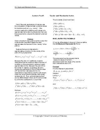
1. 45- Taylor and Maclaurin Series VU
Lecture No.45 Taylor and Maclaurin Series
One of the early applications of calculus was
the computation of approximate numerical values
for functions such as x, ln x and x
e . One
common method for obtaining such values is to
approximate the function by polynomial, then use
that polynomial to compute the desired numerical
values.
Problem
Given a function f and a point a on the x-axis, find
a polynomial of specified degree the best
approximates the function f in the “vicinity” of the
point a.
Suppose that we are interested in
approximating a function f in the vicinity of the
point a=0 by a polynomial
1 2 3
0 1 2 3( ) ....... n
nP x c c x c x c x c x= + + + + --- (1)
Because P(x) has n+1 coefficient, it seems
reasonable that we should be able to impose n+1
condition on this polynomial to achieve a good
approximation to f(x). Because the point a=0 is
the center of interest ,our strategy will be to
choose the coefficients of P(x) so that the value
of P and its first n derivates at a=0, it is
reasonable to hope that f(x) and P(x) will remain
close over some interval (possibly quite small)
centered at a=0 .Thus, we shall assume that f
can be differentiated n times at a=0 and we shall
try to find the coefficients in (1) such that
(0) (0)f p= , (0) (0)f p′ ′= ,
(0) (0)f p′′ ′′= …… (0) (0)n n
f p= --- (2)
We have
1 2 3
0 1 2 3( ) .......... n
np x c c x c x c x c x= + + + +
3 1
1 2 3( ) 2 3 ........... n
np x c x c x c x nc x −
′ = + + + +
2
2 3( ) 2 3.2 .......... ( 1) n
np x c c x n n c x −
′′ = + + + −
3
3( ) 3.2 .......... ( 1)( 2) n
np x c n n n c x −
′′′ = + + − −
( ) ( 1)( 2).......(1)n
np x n n n c= − −
Thus to satisfy (2) we must have
0
1
2 2
3 3
(0) (0)
(0) (0)
(0) (0) 2 2!
(0) (0) 3.2 3!
(0) (0) ( 1)( 2).......(1) !n n
n n
f p c
f p c
f p c c
f p c c
f p n n n c n c
= =
′ ′= =
′′ ′′= = =
′′′ ′′′= = =
= = − − =
MACLAURIN POLYNOMIALS
If f can be differentiated n times at 0, then we define
the nth Maclaurin Polynomial for f to be
2
3
(0)
( ) (0) (0)
2!
(0) (0)
........
3! !
n
n
n
f
p x f f x x
f f
x x
n
′′
′= + + +
′′′
+ +
This polynomial has the property that its
value and values of its first n
derivatives match the values of f(x) and its
first n derivatives when x=0
Example
Find the Maclaurin polynomials
0 1 2 3, , , x
nP p p p and p for e
Solution:
Let f(x) = x
e
Thus
( ) ( ) ( ) ..... ( )n x
f x f x f x f x e′ ′′ ′′′= = = = =
and
0
(0) (0) (0) ..... (0) 1n
f f f f e′ ′′ ′′′= = = = = =
© Copyright Virtual University of Pakistan
1

2. 45- Taylor and Maclaurin Series VU
Therefore
0
1
2
2
2
2
2
( ) (0) 1
( ) (0) (0) 1
(0)
( ) (0) (0) 1
2! 2!
(0) (0)
( ) (0) (0) ....
2! !
1 ........
2! !
n
n
n
n
p x f
p x f f x x
f x
p x f f x x x
f f
p x f f x x x
n
x x
x
n
= =
′= + = +
′′
′= + + = + +
′′
′= + + + +
= + + + +
Graphs of ex
and first four
Maclaurin polynomials are shown here. Note that
the graphs of P1(x), P2(x), P3(x) are virtually
indistinguishable from the graph of ex
near the
origin, so these polynomials are good
approximations of ex
near the origin. But away
from origin it does not give good approximation.
To obtain polynomial approximations of f(x) that
have their best accuracy near a general point
x=a, it will be convenient to express polynomials
in power of x-a, so that they have the form
Definition 11.9.2
If f can be differentiated n times at 0, then we define
the nth Taylor polynomial for f about x=a to be
2( )
( ) ( ) ( )( ) ( )
2!
( )
.... ( )
!
n
n
n
f a
p x f a f a x a x a
f a
x a
n
′′
′= + − + −
+ + −
Taylor and Maclaurin series
For a fixed value of x near a, one would expect that
the approximation of f(x) by its Taylor polynomial pn(x)
about x=a should improve as n increases .Since
increasing n has the effect of matching higher and
higher derivatives of f(x) with those of pn(x) at x=a.
Indeed, it seems plausible that one might be able to
achieve any desired degree of accuracy by choosing
n sufficiently large; that is the value of pn(x) might
actually converge to f(x) as
Definition 11.9.3
If f has the derivatives of all orders at a , then we
define the Taylor series for f about x=a to be
0
2
( )
( ) ( ) ( )( )
2
( ) ( )
( ) ... ( ) ...
2! !
k
k
k
k
k
f a
x a f a f a x a
f a f a
x a x a
k
∞
=
′− = + −
′′
+ − + + − +
∑
In the special case where a=0 , the Taylor series for f
is called Maclaurin series for f
Example
Find the Maclaurin Series for
)
) sin
x
a e
b x
Solution
The nth Maclaurin polynomial for x
e is
© Copyright Virtual University of Pakistan
2

3. 45- Taylor and Maclaurin Series VU
2
0
1 ...........
! 2! !
k k
k
x x x
x
k n
∞
=
= + + + +∑
Thus the Maclaurin series for x
e is
2
0
1 ..... ......
! 2! !
k k
k
x x x
x
k n
∞
=
= + + + + +∑
(b) Let ( ) sinf x x=
( ) sin (0) 0
( ) cos (0) 1
( ) sin (0) 0
( ) cos (0) 1
f x x f
f x x f
f x x f
f x x f
= =
′ ′= =
′′ = − =
′′′ = − = −
Since ( ) sin ( )f x x f x′′′′ = = the pattern 0, 1,
0,-1 will repeat over and over as we evaluate
successive derivatives at 0.
Therefore the successive Maclaurin
polynomials for sin x are
0
1
2
3
3
3
4
3 5
5
3 5
6
3 5 7
7
( ) 0
( ) 0
( ) 0 0
( ) 0 0
3!
( ) 0 0 0
3!
( ) 0 0 0
3! 5!
( ) 0 0 0 0
3! 5!
( ) 0 0 0 0
3! 5! 7!
p x
p x x
p x x
x
p x x
x
p x x
x x
p x x
x x
p x x
x x x
p x x
=
= +
= + +
= + + −
= + + − +
= + + − + +
= + + − + + +
= + + − + + + −
Because of the zero terms, each even-numbered
Maclaurin polynomial after 0 ( )p x is the same
as the odd-number Maclaurin polynomial; that is
2 1 2 2
3 5 7 2 1
( ) ( )
...... ( 1)
3! 5! 7! (2 1)!
n n
n
n
p x p x
x x x x
x
n
+ = +
+
=
= − + − + + −
+
fo
r n=0,1,2,3,4,…………….
Thus the Maclaurin series for sin x is
2 1
0
3 5 7 2 1
( 1)
(2 1)!
... ( 1) ...
3! 5! 7! (2 1)!
k
k
k
k
k
x
k
x x x x
x
k
+∞
=
+
−
+
= − + − + + − +
+
∑
© Copyright Virtual University of Pakistan
3