Learning Algorithms For Life Scientists

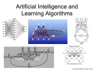
Artificial Intelligence and Learning Algorithms Presented By Brian M. Frezza 12/1/05

Game Plan
What’s a Learning Algorithm?
Why should I care?
Biological parallels
Real World Examples
Getting our hands dirty with the algorithms
Bayesian Networks
Hidden Markov Models
Genetic Algorithms
Neural Networks
Artificial Neural Networks Vs Neuron Biology
“ Fraser’s Rules”
Frontiers in AI

Hard Math

What’s a Learning Algorithm?
“An algorithm which predicts data’s future behavior based on its past performance.”
Programmer can be ignorant of the data’s trends.
Not rationally designed!
Training Data
Test Data

Why do I care?
Use In Informatics
Predict trends in “fuzzy” data
Subtle patterns in data
Complex patterns in data
Noisy data
Network inference
Classification inference
Analogies To Chemical Biology
Evolution
Immunological Response
Neurology
Fundamental Theories of Intelligence
That’s heavy dude

Street Smarts
CMU’s Navlab-5 (No Hands Across America)
1995 Neural Network Driven Car
Pittsburgh to San Diego: 2,797 miles (98.2%)
Single hidden layer backpropagation network!
Subcellular location through fluorescence
“ A Neural network classifier capable of recognizing the patterns of all major subcellular structures in fluorescence microscope images of HeLa cells” M. V. Boland, and R. F. Murphy, Bioinformatics ( 2001 ) 17( 12 ), 1213-1223
Protein secondary structure prediction
Intron/Exon predictions
Protein/Gene network inference
Speech recognition
Face recognition

The Algorithms
Bayesian Networks
Genetic Algorithms
Neural Networks

Bayesian Networks: Basics
Requires models of how data behaves
Set of Hypothesis: {H}
Keeps track of likelihood of each model being accurate as data becomes available
P(H)
Predicts as a weighted average
P(E) = Sum( P(H)*H(E) )

Bayesian Network Example
What color hair will Paul Schaffer’s
kids have if he marries Redhead ?
Hypothesis
H a (rr) rr x rr : 100% Redhead
H b (Rr) rr x R r : 50% Redhead 50% Not
H c (RR) rr x RR: 100% Not
Initially clueless:
So P(H a ) = P(H b ) = P(H c ) = 1/3

Bayesian Network: Trace H a : 100% Redhead H b : 50% Redhead 50% Not H c : 100% Not Redhead 0 Not 0 Hypothesis History Likelihood's = P( red |H a )*P(H a ) + P( red |H b )*P(H b ) + P( red |H c )*P(H c ) = (1)*(1/3) + (1/2)*(1/3) + (0)(1/3) =(1/2) Prediction: Will their next kid be a Redhead ? 1/3 1/3 1/3 P(H c ) P(H b ) P(H a )

Bayesian Network:Trace H a : 100% Redhead H b : 50% Redhead 50% Not H c : 100% Not Redhead 1 Not 0 Hypothesis History Likelihood's = P( red |H a )*P(H a ) + P( red |H b )*P(H b ) + P( red |H c )*P(H c ) = (1)*(1/2) + (1/2)*(1/2) + (0)(1/3) =(3/4) Prediction: Will their next kid be a Redhead ? 0 1/2 1/2 P(H c ) P(H b ) P(H a )

Bayesian Network: Trace H a : 100% Redhead H b : 50% Redhead 50% Not H c : 100% Not Redhead 2 Not 0 Hypothesis History Likelihood's = P( red |H a )*P(H a ) + P( red |H b )*P(H b ) + P( red |H c )*P(H c ) = (1)*(3/4) + (1/2)*(1/4) + (0)(1/3) =(7/8) Prediction: Will their next kid be a Redhead ? 0 1/4 3/4 P(H c ) P(H b ) P(H a )

Bayesian Network: Trace H a : 100% Redhead H b : 50% Redhead 50% Not H c : 100% Not Redhead 3 Not 0 Hypothesis History Likelihood's = P( red |H a )*P(H a ) + P( red |H b )*P(H b ) + P( red |H c )*P(H c ) = (1)*(7/8) + (1/2)*(1/8) + (0)(1/3) =(15/16) Prediction: Will their next kid be a Redhead ? 0 1/8 7/8 P(H c ) P(H b ) P(H a )

Bayesian Networks Notes
Never reject hypothesis unless directly disproved
Learns based on rational models of behavior
Models can be extracted!
Programmer needs to form hypothesis beforehand.

The Algorithms
Bayesian Networks
Genetic Algorithms
Neural Networks

Hidden Markov Models(HMM)
Discrete learning algorithm
Programmer must be able to categorize predictions
HMMs also assume a model of the world working behind the data
Models are also extractable
Common Uses
Speech Recognition
Secondary structure prediction
Intron/Exon predictions
Categorization of data

Hidden Markov Models: Take a Step Back
1 st order Markov Models:
Q{States}
Pr{Transition}
Sum of all P(T) out of state = 1
Q 1 Q 4 Q 2 Q 3 P 1 P 2 1-P 1 -P 2 P 3 1-P 3 1 1-P 4 P 4

1 st order Markov Model Setup
Pick Initial state: Q 1
Pick Transition Probabilities:
For each time step
Pick a random number 0.0-1.0
Q 1 Q 4 Q 2 Q 3 P 1 P 2 1-P 1 -P 2 P 3 1-P 3 1 1-P 4 P 4 P 1 P 2 P 3 P 4 0.6 0.2 0.9 0.4

1 st order Markov Model Trace
Current State: Q 1 Time Step = 1
Transition probabilities:
Random Number:
0.22341
So Next State:
0.22341 < P 1
Take P 1
Q 2

Random Number:
0.64357
So Next State:
No Choice, P = 1
Q 3

Random Number:
0.97412
So Next State:
0.97412 > 0.9
Take 1-P 3
Q 4

I’m going to stop here.
Markov Chain:
Q 1 , Q 2 , Q 3 , Q 4

What else can Markov do?
Higher Order Models
K th order
Metropolis-Hastings
Determining thermodynamic equilibrium
Continuous Markov Models
Time step varies according to continuous distribution
Discrete model learning

Hidden Markov Models (HMMs)
A Markov Model drives the world but it is hidden from direct observation and its status must be inferred from a set of observables.
Voice recognition
Observable: Sound waves
Hidden states: Words
Intron/Exon prediction
Observable: nucleotide sequence
Hidden State: Exon, Intron, Non-coding
Secondary structure prediction for protein
Observable: Amino acid sequence
Hidden State: Alpha helix, Beta Sheet, Unstructured

Hidden Markov Models: Example
Secondary Structure Prediction
Observable States Hidden States Unstructured Alpha Helix Beta Sheet His Asp Arg Phe Ala Cis Ser Gln Glu Lys Leu Met Asn Ser Tyr Thr Ile Trp Pro Val Gly

Hidden Markov Models: Smaller Example
Exon/Intron Mapping
Hidden State Transition Probabilities Observable State Probabilities To From Hidden State Observable Starting Distribution 0.8 0.02 0.18 It 0.01 0.5 0.49 Ig 0.2 0.1 0.7 Ex It Ig Ex 0.2 0.5 0.16 0.14 It 0.25 0.25 0.25 0.25 Ig 0.14 0.11 0.42 0.33 Ex C G T A 0.01 0.89 0.1 It Ig Ex

Hidden Markov Model
How to predict outcomes from a HMM
Brute force:
Try every possible Markov chain
Which chain has greatest probability of generating observed data?
Viterbi algorithm
Dynamic programming approach

Viterbi Algorithm: Trace Hidden State Transition Probabilities Observable State Probabilities To From Hidden State Observable Starting Distribution Example Sequence: ATAATGGCGAGTG Exon = P(A|Ex) * Start Exon = 3.3*10 -2 Introgenic = P(A|Ig) * Start Ig = 2.2*10 -1 Intron = P(A|It) * Start It = 0.14 * 0.01 = 1.4*10 -3 0.8 0.02 0.18 It 0.01 0.9 0.09 Ig 0.2 0.1 0.7 Ex It Ig Ex 0.2 0.5 0.16 0.14 It 0.25 0.25 0.25 0.25 Ig 0.14 0.11 0.42 0.33 Ex C G T A 0.01 0.89 0.1 It Ig Ex G T A G A G C G G T A A T 1.4*10 -3 2.2*10 -1 3.3*10 -2 A Intron Introgenic Exon

Viterbi Algorithm: Trace Hidden State Transition Probabilities Observable State Probabilities To From Hidden State Observable Starting Distribution Example Sequence: ATAATGGCGAGTG Exon = Max( P(Ex|Ex)*P n-1 (Ex), P(Ex|Ig)*P n-1 (Ig), P(Ex|It)*P n-1 (It) ) *P(T|Ex) = 4.6*10 -2 Introgenic =Max( P(Ig|Ex)*P n-1 (Ex), P(Ig|Ig)*P n-1 (Ig), P(Ig|It)*P n-1 (It) ) * P(T|Ig) = 2.8*10 -2 Intron = Max( P(It|Ex)*P n-1 (Ex), P(It|Ig)*P n-1 (Ig), P(It,It)*P n-1 (It) ) * P(T|It) = 1.1*10 -3 0.8 0.02 0.18 It 0.01 0.5 0.49 Ig 0.2 0.1 0.7 Ex It Ig Ex 0.2 0.5 0.16 0.14 It 0.25 0.25 0.25 0.25 Ig 0.14 0.11 0.42 0.33 Ex C G T A 0.01 0.89 0.1 It Ig Ex G T A G A G C G G T A A 1.1*10 -3 2.8*10 -2 4.6*10 -2 T 1.4*10 -3 2.2*10 -1 3.3*10 -2 A Intron Introgenic Exon

Viterbi Algorithm: Trace Hidden State Transition Probabilities Observable State Probabilities To From Hidden State Observable Starting Distribution Example Sequence: ATAATGGCGAGTG Exon = Max( P(Ex|Ex)*P n-1 (Ex), P(Ex|Ig)*P n-1 (Ig), P(Ex|It)*P n-1 (It) ) *P(T|Ex) = 1.1*10 -2 Introgenic =Max( P(Ig|Ex)*P n-1 (Ex), P(Ig|Ig)*P n-1 (Ig), P(Ig|It)*P n-1 (It) ) * P(T|Ig) = 3.5*10 -3 Intron = Max( P(It|Ex)*P n-1 (Ex), P(It|Ig)*P n-1 (Ig), P(It,It)*P n-1 (It) ) * P(T|It) = 1.3*10 -3 0.8 0.02 0.18 It 0.01 0.5 0.49 Ig 0.2 0.1 0.7 Ex It Ig Ex 0.2 0.5 0.16 0.14 It 0.25 0.25 0.25 0.25 Ig 0.14 0.11 0.42 0.33 Ex C G T A 0.01 0.89 0.1 It Ig Ex G T A G A G C G G T A 1.3*10 -3 3.5*10 -3 1.1*10 -2 A 1.1*10 -3 2.8*10 -2 4.6*10 -2 T 1.4*10 -3 2.2*10 -1 3.3*10 -2 A Intron Introgenic Exon

Viterbi Algorithm: Trace Hidden State Transition Probabilities Observable State Probabilities To From Hidden State Observable Starting Distribution Example Sequence: ATAATGGCGAGTG Exon = Max( P(Ex|Ex)*P n-1 (Ex), P(Ex|Ig)*P n-1 (Ig), P(Ex|It)*P n-1 (It) ) *P(T|Ex) Introgenic =Max( P(Ig|Ex)*P n-1 (Ex), P(Ig|Ig)*P n-1 (Ig), P(Ig|It)*P n-1 (It) ) * P(T|Ig) Intron = Max( P(It|Ex)*P n-1 (Ex), P(It|Ig)*P n-1 (Ig), P(It,It)*P n-1 (It) ) * P(T|It) 0.8 0.02 0.18 It 0.01 0.5 0.49 Ig 0.2 0.1 0.7 Ex It Ig Ex 0.2 0.5 0.16 0.14 It 0.25 0.25 0.25 0.25 Ig 0.14 0.11 0.42 0.33 Ex C G T A 0.01 0.89 0.1 It Ig Ex G T A G A G C G G T 2.9*10 -4 4.3*10 -4 2.4*10 -3 A 1.3*10 -3 3.5*10 -3 1.1*10 -2 A 1.1*10 -3 2.8*10 -2 4.6*10 -2 T 1.4*10 -3 2.2*10 -1 3.3*10 -2 A Intron Introgenic Exon

Viterbi Algorithm: Trace Hidden State Transition Probabilities Observable State Probabilities To From Hidden State Observable Starting Distribution Example Sequence: ATAATGGCGAGTG Exon = Max( P(Ex|Ex)*P n-1 (Ex), P(Ex|Ig)*P n-1 (Ig), P(Ex|It)*P n-1 (It) ) *P(T|Ex) Introgenic =Max( P(Ig|Ex)*P n-1 (Ex), P(Ig|Ig)*P n-1 (Ig), P(Ig|It)*P n-1 (It) ) * P(T|Ig) Intron = Max( P(It|Ex)*P n-1 (Ex), P(It|Ig)*P n-1 (Ig), P(It,It)*P n-1 (It) ) * P(T|It) 0.8 0.02 0.18 It 0.01 0.5 0.49 Ig 0.2 0.1 0.7 Ex It Ig Ex 0.2 0.5 0.16 0.14 It 0.25 0.25 0.25 0.25 Ig 0.14 0.11 0.42 0.33 Ex C G T A 0.01 0.89 0.1 It Ig Ex G T A G A G C G G 7.8*10 -5 6.1*10 -5 7.2*10 -4 T 2.9*10 -4 4.3*10 -4 2.4*10 -3 A 1.3*10 -3 3.5*10 -3 1.1*10 -2 A 1.1*10 -3 2.8*10 -2 4.6*10 -2 T 1.4*10 -3 2.2*10 -1 3.3*10 -2 A Intron Introgenic Exon

Viterbi Algorithm: Trace Hidden State Transition Probabilities Observable State Probabilities To From Hidden State Observable Starting Distribution Example Sequence: ATAATGGCGAGTG Exon = Max( P(Ex|Ex)*P n-1 (Ex), P(Ex|Ig)*P n-1 (Ig), P(Ex|It)*P n-1 (It) ) *P(T|Ex) Introgenic =Max( P(Ig|Ex)*P n-1 (Ex), P(Ig|Ig)*P n-1 (Ig), P(Ig|It)*P n-1 (It) ) * P(T|Ig) Intron = Max( P(It|Ex)*P n-1 (Ex), P(It|Ig)*P n-1 (Ig), P(It,It)*P n-1 (It) ) * P(T|It) 0.8 0.02 0.18 It 0.01 0.5 0.49 Ig 0.2 0.1 0.7 Ex It Ig Ex 0.2 0.5 0.16 0.14 It 0.25 0.25 0.25 0.25 Ig 0.14 0.11 0.42 0.33 Ex C G T A 0.01 0.89 0.1 It Ig Ex G T A G A G C G 7.2*10 -5 1.8*10 -5 5.5*10 -5 G 7.8*10 -5 6.1*10 -5 7.2*10 -4 T 2.9*10 -4 4.3*10 -4 2.4*10 -3 A 1.3*10 -3 3.5*10 -3 1.1*10 -2 A 1.1*10 -3 2.8*10 -2 4.6*10 -2 T 1.4*10 -3 2.2*10 -1 3.3*10 -2 A Intron Introgenic Exon

Viterbi Algorithm: Trace Hidden State Transition Probabilities Observable State Probabilities To From Hidden State Observable Starting Distribution Example Sequence: ATAATGGCGAGTG Exon = Max( P(Ex|Ex)*P n-1 (Ex), P(Ex|Ig)*P n-1 (Ig), P(Ex|It)*P n-1 (It) ) *P(T|Ex) Introgenic =Max( P(Ig|Ex)*P n-1 (Ex), P(Ig|Ig)*P n-1 (Ig), P(Ig|It)*P n-1 (It) ) * P(T|Ig) Intron = Max( P(It|Ex)*P n-1 (Ex), P(It|Ig)*P n-1 (Ig), P(It,It)*P n-1 (It) ) * P(T|It) 0.8 0.02 0.18 It 0.01 0.5 0.49 Ig 0.2 0.1 0.7 Ex It Ig Ex 0.2 0.5 0.16 0.14 It 0.25 0.25 0.25 0.25 Ig 0.14 0.11 0.42 0.33 Ex C G T A 0.01 0.89 0.1 It Ig Ex G T A G A G C 2.9*10 -5 2.2*10 -6 4.3*10 -6 G 7.2*10 -5 1.8*10 -5 5.5*10 -5 G 7.8*10 -5 6.1*10 -5 7.2*10 -4 T 2.9*10 -4 4.3*10 -4 2.4*10 -3 A 1.3*10 -3 3.5*10 -3 1.1*10 -2 A 1.1*10 -3 2.8*10 -2 4.6*10 -2 T 1.4*10 -3 2.2*10 -1 3.3*10 -2 A Intron Introgenic Exon

Viterbi Algorithm: Trace Hidden State Transition Probabilities Observable State Probabilities To From Hidden State Observable Starting Distribution Example Sequence: ATAATGGCGAGTG Exon = Max( P(Ex|Ex)*P n-1 (Ex), P(Ex|Ig)*P n-1 (Ig), P(Ex|It)*P n-1 (It) ) *P(T|Ex) Introgenic =Max( P(Ig|Ex)*P n-1 (Ex), P(Ig|Ig)*P n-1 (Ig), P(Ig|It)*P n-1 (It) ) * P(T|Ig) Intron = Max( P(It|Ex)*P n-1 (Ex), P(It|Ig)*P n-1 (Ig), P(It,It)*P n-1 (It) ) * P(T|It) 0.8 0.02 0.18 It 0.01 0.5 0.49 Ig 0.2 0.1 0.7 Ex It Ig Ex 0.2 0.5 0.16 0.14 It 0.25 0.25 0.25 0.25 Ig 0.14 0.11 0.42 0.33 Ex C G T A 0.01 0.89 0.1 It Ig Ex 4.7*10 -10 3.6*10 -11 1.1*10 -10 G 1.2*10 -9 1.2*10 -10 1.4*10 -9 T 9.2*10 -9 4.1*10 -10 4.9* -9 A 8.2*10 -8 2.7*10 -9 8.4* -9 G 2.0*10 -7 9.1*10 -9 1.1*10 -7 A 1.8*10 -6 3.5*10 -8 9.1*10 -8 G 4.6*10 -6 2.8*10 -7 7.2*10 -7 C 2.9*10 -5 2.2*10 -6 4.3*10 -6 G 7.2*10 -5 1.8*10 -5 5.5*10 -5 G 7.8*10 -5 6.1*10 -5 7.2*10 -4 T 2.9*10 -4 4.3*10 -4 2.4*10 -3 A 1.3*10 -3 3.5*10 -3 1.1*10 -2 A 1.1*10 -3 2.8*10 -2 4.6*10 -2 T 1.4*10 -3 2.2*10 -1 3.3*10 -2 A Intron Introgenic Exon

How to Train an HMM
The forward-backward algorithm
Ugly probability theory math:
Starts with an initial guess of parameters
Refines parameters by attempting to reduce the errors it provokes with fitted to the data.
Normalized probability of the “Forward probability” of arriving at the state given the observable cross multiplied by the backward probability of generating that observable given the parameter.
CENSORED

The Algorithms
Bayesian Networks
Genetic Algorithms
Neural Networks

Genetic Algorithms
Individuals are series of bits which represent candidate solutions
Functions
Structures
Images
Code
Based on Darwin evolution
individuals mate, mutate, and are selected based on a Fitness Function

Genetic Algorithms
Encoding Rules
“ Gray” bit encoding
Bit distance proportional to value distance
Selection Rules
Digital / Analog Threshold
Linear Amplification Vs Weighted Amplification
Mating Rules
Mutation parameters
Recombination parameters

Genetic Algorithms
When are they useful?
Movements in sequence space are funnel shaped with fitness function
Systems where evolution actually applies!
Examples
Medicinal chemistry
Protein folding
Amino acid substitutions
Membrane trafficking modeling
Ecological simulations
Linear Programming
Traveling salesman

The Algorithms
Bayesian Networks
Genetic Algorithms
Neural Networks

Neural Networks
1943 McCulloch and Pitts Model of how Neurons process information
Field immediately splits
Studying brain’s
Neurology
Studying artificial intelligence
Neural Networks

Neural Networks: A Neuron, Node, or Unit Σ ( W )- W 0,c Activation Function Output W a,c W b,c W 0,c (Bias) W c, n a z (Bias)

Neural Networks: Activation Functions Sigmoid Function (logistic function) Threshold Function Zero point set by bias In In out out +1 +1

Threshold Functions can make Logic Gates with Neurons! Logical And W 0,c = 1.5 W b,c = 1 W a,c = 1 A B Σ ( W )- W 0,c a z (Bias) Output If ( Σ (w) – W o,c > 0 ) Then FIRE Else Don’t (Bias) 0 0 0 0 1 1 0 1 ∩

And Gate: Trace W 0,c = 1.5 W b,c = 1 W a,c = 1 -1.5 Off Off Off -1.5 < 0 (Bias)

And Gate: Trace W 0,c = 1.5 W b,c = 1 W a,c = 1 -0.5 On Off Off -0.5 < 0 (Bias)

And Gate: Trace W 0,c = 1.5 W b,c = 1 W a,c = 1 -0.5 Off On Off -0.5 < 0 (Bias)

And Gate: Trace W 0,c = 1.5 W b,c = 1 W a,c = 1 0.5 On On On 0.5 > 0 (Bias)

Threshold Functions can make Logic Gates with Neurons! W 0,c = 0.5 W b,c = 1 W a,c = 1 A Σ ( W )- W 0,c a z (Bias) If ( Σ (w) – W o,c > 0 ) Then FIRE Else Don’t (Bias) Logical Or B 0 1 0 1 1 1 0 1 U

Or Gate: Trace W 0,c = 0.5 W b,c = 1 W a,c = 1 -0.5 Off Off Off -0.5 < 0 (Bias)

Or Gate: Trace W 0,c = 0.5 W b,c = 1 W a,c = 1 0.5 On Off On 0.5 > 0 (Bias)

Or Gate: Trace W 0,c = 0.5 W b,c = 1 W a,c = 1 0.5 Off On On 0.5 > 0 (Bias)

Or Gate: Trace W 0,c = 0.5 W b,c = 1 W a,c = 1 1.5 On On On 1.5 > 0 (Bias)

Threshold Functions can make Logic Gates with Neurons! W 0,c = -0.5 W a,c = -1 Σ ( W )- W 0,c a z (Bias) If ( Σ (w) – W o,c > 0 ) Then FIRE Else Don’t (Bias) Logical Not 1 0 0 1 !

Not Gate: Trace W 0,c = -0.5 W a,c = -1 -0.5 Off On 0.5 > 0 (Bias) 0 – (-0.5) = 0.5

Not Gate: Trace W 0,c = -0.5 W a,c = -1 -0.5 On Off -0.5 < 0 (Bias) -1 – (-0.5) = -0.5

Feed-Forward Vs. Recurrent Networks
Feed-Forward
No Cyclic connections
Function of its current inputs
No internal state other then weights of connections
“ Out of time”
Recurrent
Cyclic connections
Dynamic behavior
Stable
Oscillatory
Chaotic
Response depends on current state
“ In time”
Short term memory!

Feed-Forward Networks
“ Knowledge” is represented by weight on edges
Modeless!
“ Learning” consists of adjusting weights
Customary Arrangements
One Boolean output for each value
Arranged in Layers
Layer 1 = inputs
Layer 2 to (n-1) = Hidden
Layer N = outputs
“ Perceptron” 2 layer Feed-Forward network

Layers Input Output Hidden layer

Perceptron Learning
Gradient Decent used to reduce error
Essentially:
New Weight = Old Weight + adjustment
Adjustment = α X error X input X d( activation function )
α = Learning Rate
CENSORED

Hidden Network Learning
Back-Propagation
Essentially:
Start with Gradient Decent from output
Assign “blame” to inputting neurons proportional to their weights
Adjust weights at previous level using Gradient decent based on “blame”
CENSORED

They don’t get it either: Issues that aren’t well understood
α (Learning Rate)
Depth of network (number of layers)
Size of hidden layers
Overfitting
Cross-validation
Minimum connectivity
Optimal Brain Damage Algorithm
No extractable model!

How Are Neural Nets Different From My Brain?
Neural nets are feed forward
Brains can be recurrent with feedback loops
Neural nets do not distinguish between + or – connections
In brains excitatory and inhibitory neurons have different properties
Inhibitory neurons short-distance
Neural nets exist “Out of time”
Our brains clearly do exist “in time”
Neural nets learn VERY differently
We have very little idea how our brains are learning
“ Fraser’s” Rules “ In theory one can, of course, implement biologically realistic neural networks, but this is a mammoth task. All kinds of details have to be gotten right, or you end up with a network that completely decays to unconnectedness, or one that ramps up its connections until it basically has a seizure.”

Frontiers in AI
Applications of current algorithms
New algorithms for determining parameters from training data
Backward-Forward
Backpropagation
Better classification of the mysteries of neural networks
Pathology modeling in neural networks
Evolutionary modeling

http://www.weebly.com	15
http://www.slideshare.net	4
http://kauffmannschuler.weebly.com	4

Learning Algorithms For Life Scientists

by Brian Frezza on Jan 14, 2009

Accessibility

Categories

Tags

Upload Details

Usage Rights

3 Embeds 23

Statistics

Learning Algorithms For Life Scientists — Presentation Transcript