Surface hydrology

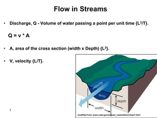
1. • Discharge, Q - Volume of water passing a point per unit time {L3/T}.
• A, area of the cross section (width x Depth) {L2}.
• V, velocity {L/T}.
modified from www.usda.gov/stream_restoration/chap1.html
Flow in Streams
Q = v * A
1

2. Velocity profiles
2

3. Stream velocity profiles
Length of arrows represent
stream velocity at different
locations and depths
across a typical
meandering stream
3

4. Meandering stream profile
4

5. Velocity distribution in a channel
How to measure average velocity ?
Q = vA
Table 3 – SonTek Formulation of ISO Uncertainty For Number of Velocity Measurements
Number of Measurements Uncertainty
1 7.5%
2 3.5%
3 3.0%
4 2.7%
5 or more 2.5%
5

6. Methods for measuring discharge
Theoretical methods
Models (simple)- Manning
Models (complex)-
Practical
Velocity-area – velocity meters
Velocity- tracer addition
Weirs Discharge stations- & Rating curves
Theoretical methods
Models (simple)- Manning
Models (complex)- numerical models
Practical
Velocity-area – velocity meters
Velocity- tracer addition
Weirs
Discharge stations- & Rating curves

7. Manning’s Equation
• In 1889 Irish Engineer, Robert Manning presented the formula:
2
1
3
2
1
S
R
n
v 
v is the flow velocity (m/s)
n is known as Manning’s n and is a coefficient of roughness (s/m1/3)
R is the hydraulic radius (A/P) where P is the wetted perimeter (m)
S is the channel bed slope as a fraction
The Manning’s equation helps to explain why velocity usually increases along the
stream length, even as the gradient decreases. Channel depth generally is greater
and substrates are finer as one proceeds downstream, hence resistance decreases
longitudinally and this offsets the effect of reduction in slope.
7

8. Manning’s n Roughness Coefficient
Type of Channel and Description Minimum Normal Maximum
Streams
Streams on plain
Clean, straight, full stage, no rifts or deep pools 0.025 0.03 0.033
Clean, winding, some pools, shoals, weeds &
stones
0.033 0.045 0.05
Same as above, lower stages and more stones 0.045 0.05 0.06
Sluggish reaches, weedy, deep pools 0.05 0.07 0.07
Very weedy reaches, deep pools, or floodways 0.075 0.1 0.15
with heavy stand of timber and underbrush
Mountain streams, no vegetation in channel, banks
steep, trees & brush along banks submerged at
high stages
Bottom: gravels, cobbles, and few boulders 0.03 0.04 0.05
Bottom: cobbles with large boulders 0.04 0.05 0.07
(
Chow, 1959
)
8

9. Impact of channel roughness and structure on flow
Smooth, half circle- low resistance fast velocity
Smooth, wide channel- high resistance slow velocity
Rough, half circle- high resistance slow velocity
9

10. Example Problem
Velocity & Discharge
 Channel geometry known
 Depth of flow known
 Determine the flow velocity and discharge
6 m
0.33 m
 Bed slope of 0.002 m/m
 Stream bottom: gravels, cobbles, and few boulders
Culvert Design
10

11. Solution
• Q = vA
•
• R= A/P
• A = width x depth = 6m x 0.33 m = 1.98 m2
• P= 6 m + 0.33 m + 0.33 m = 6.66 m.
• R= 1.98/6.66 = 0.3 m
• S = 0.002 m/m (given) and n = 0.04 (from the
table)
• v = (1/0.04)(0.3)2/3(0.002)1/2 = 0.5 m/s
• Q = vA=0.5x6.66= 0.99 m3/s
2
1
3
2
1
S
R
n
v 
11

12. • Measure V at 0.2 and 0.8 of depth
• Average V and multiply by (D width * depth)
• Sum up across stream to get total FLOW
• Q = S (Vi Di DWi)
Velocity-area method
In a deep stream subsection, the average velocity is estimated by measurements
at 20% depth (0.2D) and 80% depth (0.8D).
In a shallow stream subsection where measurement at two depths is not feasible,
the average velocity is determined by measuring velocity at 60% of the depth
(0.6D(
12

13. Velocity (wading instruments)
velocity meters
Electromagnetic
velocity meter
Mechanical velocity meter Acoustic Doppler Velocity
meter (ADV)
Faraday's Formula: E is proportional to V x B x D where:
E = The voltage generated in a conductor
V = The velocity of the water
B = The magnetic field strength
D = The length of the conductor (instrument design)

14. Acoustic velocimeters
Acoustic Doppler Velocity
meter (ADV)
Let’s go a bit more deeply into the
principle of the ADV, which we will use
in the field.
The ADV measures the velocity of
water using a physical principle called
the Doppler effect.
• If a source of sound is moving
relative to the receiver, the frequency
of the sound at the
receiver is shifted from the transmit
frequency.
• For Doppler current meters, we look
at the reflection of sound from
particles in the water.
• The change in frequency is
proportional to the velocity of the
water.

15. Acoustic Doppler current profiler- ADCP
Source- USGS

16. Acoustic Doppler current profiler- ADCP
River Surveyor by Sontek or
equivalent products by Nortek or
Teledyne-Tekmar

17. Weirs, flumes, and discharge
measurement at gaging stations
17

18. https://www.ott.com/products/water-flow-3/ott-cable-way-
systems-1762/
Other methods to measure discharge
Costa et al. 2006 (WRR)
Radar

19. Q -discharge (L3/t)
Ct- concentration of the tracer (Mass/ L3)
Vt- volume of the tracer (L3)
C- concentration downstream (Mass/ L3)
Cb- background concentration (Mass/ L3)
0
20
40
60
80
100
120
140
160
0.00 100.00 200.00 300.00 400.00 500.00 600.00 700.00 800.00 900.00
EC
(microsimens/cm)
Time from injection, s
Tracer-Dilution Method
Mass

20. 0.00
10.00
20.00
30.00
40.00
50.00
60.00
0.00 200.00400.00600.00800.001000.00
Concentration
Above
Bkg,
mg/l
Time from injection, s
0
20
40
60
80
100
120
140
160
0.00 200.00 400.00 600.00 800.00 1000.00
EC
(microsimens/cm)
Time from injection, s
Tracer-Dilution Method
Solution
1) Measure EC downstream
2) Convert EC to salt concentration
3) Plot the breakthrough curve (BTC)
4) Remove background levels from the BTC
5) Integrate the are under the curve to get the
Chloride mass
Mass

21. Stage -Discharge Relationship
21
• Need to:
1. Measuring the stage (G) and discharge.
2. Prepare a stage discharge “rating curve”
• For a gauging section of the channel, the measured
values of discharge are plotted against the
corresponding stages.
• The flow can be control by G-Q curve when:
1. G-Q is constant with time (permanent)
2. G-Q is vary with time (shifting control)

22. Permanent control
22
• Most of streams and rivers follow the permanent
type and the G-Q curve can be represented by:
• Q = stream discharge
• G = gauge height
• a = a constant of stage at zero discharge
• Cr & B = rating constants

23. 23
How real data look like?

24. 24
• Straight lines is drown in logarithmic plot for (G-Q)
• Then Cr & B can be determined by the least
square error method
Cont.


25. Stage for zero discharge (a)
25
• It is hypothetical parameter and can’t be measured
Method 1
 Plot Q vs. G on arithmetic scale
 Draw the best fit curve
 Select the value of (a) where Q = 0
 Use (a) value and verify wither the data at
log(Q) vs. log(G-a) indicate a straight line
 Trial and error find acceptable value of (a)

26. Stage for zero discharge (a)
26
Method 2 (Running’s Method)
 Plot Q&G on arithmetic scale and select the
best fit curve
 Select three points (A,B and C) as
 Draw vertical lines from (A,B and C) and
horizontal lines from (B and C)
 Two straight lines ED and BA intersect at F
(value of a)
See graphic solution on the next page

27. Stage for zero discharge (a)
27
Method 2 (Running’s Method)
A= 16.5

28. Summary
1. We have learned most of the s techniques for measuring flow in streams
2. Each method has advantages and disadvantages.
3. We select the method based on what we need and what can be done
(budget…).
4. Next phase….. Try and use the methods in the stream. This includes:
- ADV
-ADCP
-Tracer dilution
-Rating curve