
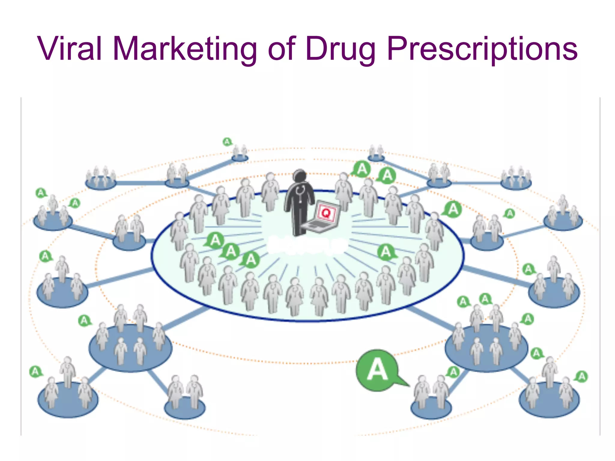
![Propagation Drug Prescriptions
• nodes = physicians; links = ties.
• Question: does contagion work through the network?
• answer: affirmative.
• volume of usage (prescription of drug) controls contagion
more than whether peer prescribed drug.
• genuine social contagion found to be at play, even after
controlling for mass media marketing efforts, and global
network wide changes.
• targeting sociometric opinion leaders definitely beneficial.
[R. Iyengar, et al. Opinion Leadership and Social Contagion in New Product
Diffusion. Marketing Science, 30(2):195–212, 2011.]](https://image.slidesharecdn.com/wsdm2018tutorial-180611122200/75/WSDM-2018-Tutorial-on-Influence-Maximization-in-Online-Social-Networks-14-2048.jpg)
![Analysis workflow for Saccharomyces cerevisiae.
IM and Yeast Cell Cycle Regulation
[Gibbs DL, Schmulevich I (2017). Solving the influence maximization problem reveals regulatory
organization of the yeast cell cycle. PLOS Compt.Biol 13(6). e1005591. https://doi.org/10.1371/journal.pcbi.
1005591].](https://image.slidesharecdn.com/wsdm2018tutorial-180611122200/75/WSDM-2018-Tutorial-on-Influence-Maximization-in-Online-Social-Networks-15-2048.jpg)
![Topology of influential nodes.
[Gibbs DL, Shmulevich I (2017) Solving the influence maximization problem reveals regulatory organization of the yeast cell cycle.
PLOS Computational Biology 13(6): e1005591. https://doi.org/10.1371/journal.pcbi.1005591]
http://journals.plos.org/ploscompbiol/article?id=10.1371/journal.pcbi.1005591
IM and Yeast Cell Cycle Regulation](https://image.slidesharecdn.com/wsdm2018tutorial-180611122200/75/WSDM-2018-Tutorial-on-Influence-Maximization-in-Online-Social-Networks-16-2048.jpg)
![Social Influence in Political Mobilization
• is influence in OSN real or as effective as
offline SN?
• what about weak ties?
• can OSN be used to harness behavioral
change at scale?
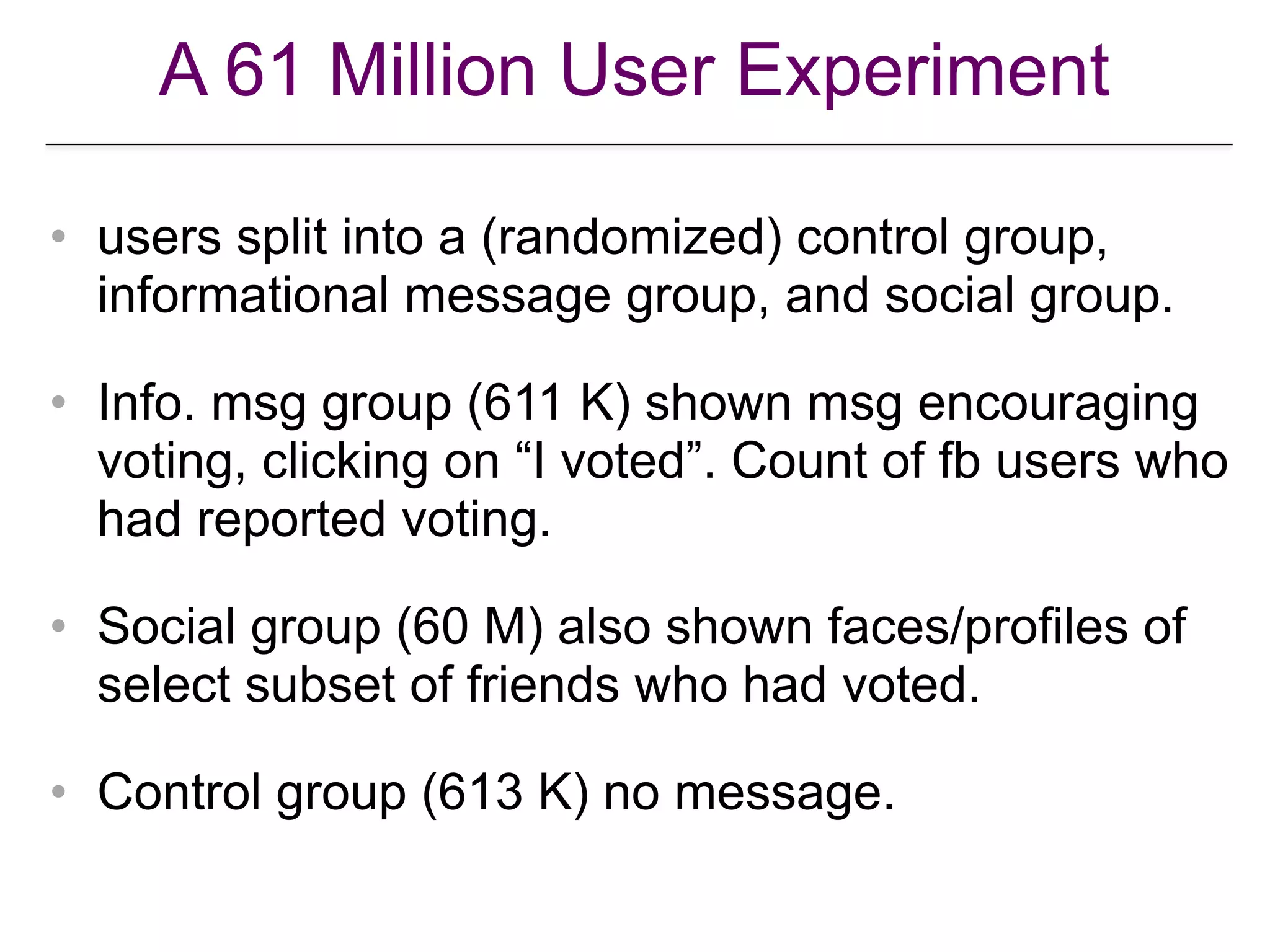
• A large scale (61M users) study on
Facebook.
[RM. Bond et al. A 61-million … poitical mobilization. Nature 489, 295-298
(2012) doi:10.1038/nature11421].](https://image.slidesharecdn.com/wsdm2018tutorial-180611122200/75/WSDM-2018-Tutorial-on-Influence-Maximization-in-Online-Social-Networks-18-2048.jpg)
![A 61 Million User Experiment
[RM Bond et al. Nature 489, 295-298 (2012) doi:10.1038/nature11421].](https://image.slidesharecdn.com/wsdm2018tutorial-180611122200/75/WSDM-2018-Tutorial-on-Influence-Maximization-in-Online-Social-Networks-20-2048.jpg)
![Effect of friend’s mobilization treatment on a user’s behavior
[RM Bond et al. Nature 489, 295-298 (2012) doi:10.1038/nature11421].](https://image.slidesharecdn.com/wsdm2018tutorial-180611122200/75/WSDM-2018-Tutorial-on-Influence-Maximization-in-Online-Social-Networks-21-2048.jpg)
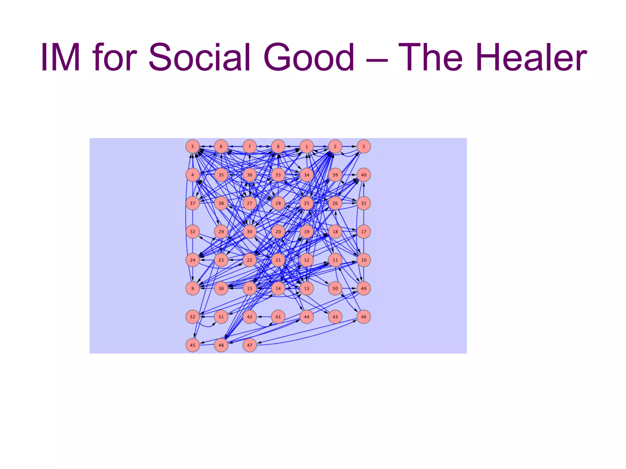
![IM for Social Good – The Healer
homeless
youth
Facebook
application
homeless
youth
.
.
.
DIME
solver
shelter
official
action
recommendation
feedback
[Amulya Yadav et al. Using Social Networks to Aid Homeless Shelters: Dynamic Influence Maximization Under
Uncertainty. Proc. Int. Conf. on Autonomous Agents and Multiagent Systems (AAMAS), 2016.]
HEALER PROJECT: http://teamcore.usc.edu/people/amulya/healer/index.html](https://image.slidesharecdn.com/wsdm2018tutorial-180611122200/75/WSDM-2018-Tutorial-on-Influence-Maximization-in-Online-Social-Networks-24-2048.jpg)
![Propagation/Diffusion Models
• How does influence/information travel?
• Deterministic versus stochastic models.
• Discrete time versus continuous time models.
• Phenomena captured: infection or product
adoption?
[W. Chen, L., and Carlos Castillo. Information and Influence Propagation in Socia
Networks. Morgan-Claypool 2013].](https://image.slidesharecdn.com/wsdm2018tutorial-180611122200/75/WSDM-2018-Tutorial-on-Influence-Maximization-in-Online-Social-Networks-26-2048.jpg)
![Independent cascade model
0.3
0.1
0.1
0.02
0.2
0.1
0.2
0.4
0.3
0.1
0.3
0.3
0.30.04
0.2
0.1
0.7
0.1
0.01
0.05
[Kempe et al. KDD 2003].
• Each edge has
influence probability .
• Seeds selected activate at
time
• At each , each active
node gets one shot at
activating its inactive
neighbor ; succeeds w.p.
and fails w.p.
• Once active, stay active.
(u,v)
puv
t = 0.
t > 0
u
v
puv (1− puv ).
similar to infection propagation.](https://image.slidesharecdn.com/wsdm2018tutorial-180611122200/75/WSDM-2018-Tutorial-on-Influence-Maximization-in-Online-Social-Networks-30-2048.jpg)
![0.3
0.1
0.1
0.2
0.2
0.3
0.2
0.4
0.3
0.1
0.3
0.3
0.30.2
0.2
0.5
0.5
0.8
0.1
0.2
0.3
0.7
0.3
0.5
0.6
0.3
0.2
0.4
0.8
Linear threshold model
[Kempe et al. KDD 2003].
• Each edge has weight
• Each node chooses a
threshold at random.
• Activate if total
influence of active
in-neighbors exceeds
node’s threshold.
(u,v)
w(u,v): w(u,v) ≤1
u
∑
similar to technology adoption or opinion propagation.](https://image.slidesharecdn.com/wsdm2018tutorial-180611122200/75/WSDM-2018-Tutorial-on-Influence-Maximization-in-Online-Social-Networks-31-2048.jpg)
![Continuous Time
• = conditional prob.
that gets the infection transmitted
from at time given that was
infected at time .
• = transmission rate
• assumed to be shift invariant:
– e.g.,
[Gomez-Rodriguez and Schölkopf. IM in continuous time diffusion networks.
ICML 2012].](https://image.slidesharecdn.com/wsdm2018tutorial-180611122200/75/WSDM-2018-Tutorial-on-Influence-Maximization-in-Online-Social-Networks-33-2048.jpg)
![Influence Maximization Defined
• Core optimization problem in IM: Given a
diffusion model M, a network G = (V,E),
model parameters, and problem parameters
(budget, time horizon [for continuous time
models only]). Find a seed set under
budget that maximizes or
(expected) spread.](https://image.slidesharecdn.com/wsdm2018tutorial-180611122200/75/WSDM-2018-Tutorial-on-Influence-Maximization-in-Online-Social-Networks-36-2048.jpg)
![Approximation of Submodular Function
Optimization
• Theorem: Let be a monotone
submodular function, with Let
and resp. be the greedy and optimal solutions.
Then
• Theorem: The spread function is monotone
and submodular under various major diffusion
models, for both discrete and continuous time.
[Nemhauser et al. An analysis of the approximations for maximizing submodular
set functions. Math. Prog., 14:265–294, 1978.]](https://image.slidesharecdn.com/wsdm2018tutorial-180611122200/75/WSDM-2018-Tutorial-on-Influence-Maximization-in-Online-Social-Networks-42-2048.jpg)
![Baseline Approximation Algorithm
Monte Carlo simulation for estimating
expected spread.
CELF leverages submodularity to save on
unnecessary evals of marginal gain.
Greedy still extremely slow on large networks.
[Leskovec et al. Cost-effective outbreak detection in networks. KDD 2007]](https://image.slidesharecdn.com/wsdm2018tutorial-180611122200/75/WSDM-2018-Tutorial-on-Influence-Maximization-in-Online-Social-Networks-44-2048.jpg)
![Heuristics
• Numerous heuristics have been proposed.
• We will discuss PMIA (IC), SimPath (LT) [if
time permits], and PMC$ (IC).
$Technically PMC is an approximation
algorithm; however, to make it scale requires
setting small parameter values which can
compromise accuracy.](https://image.slidesharecdn.com/wsdm2018tutorial-180611122200/75/WSDM-2018-Tutorial-on-Influence-Maximization-in-Online-Social-Networks-46-2048.jpg)
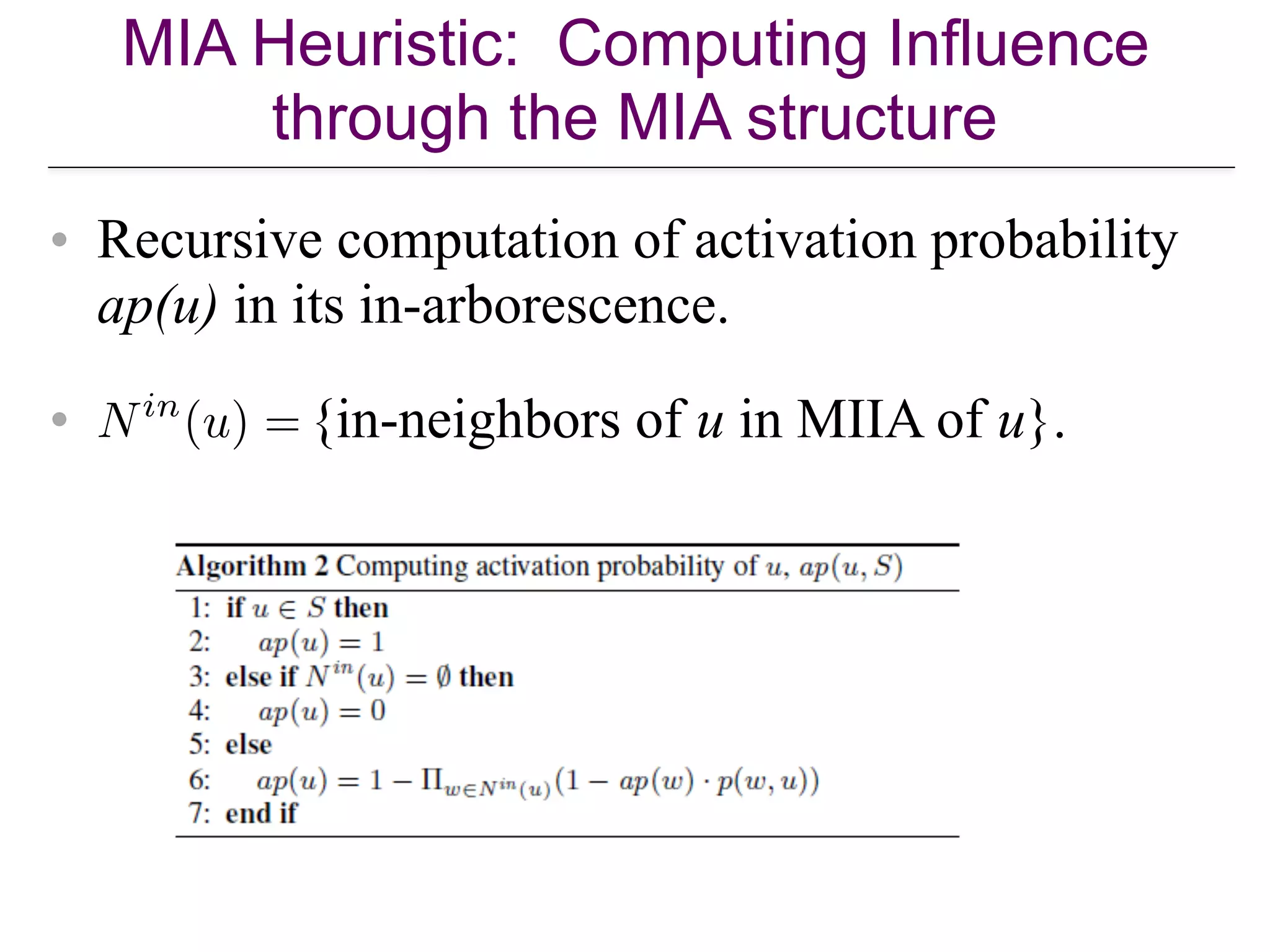
![Maximum Influence Arborescence
(MIA) Heuristic
0.3
0.1
0.1
0.02
0.2
0.1
0.2
0.4
0.3
0.1
0.3
0.3
0.3
0.04
0.2
0.1
0.7
0.1
0.01
0.05
• For given node v, for each
node u, compute the max.
influence path from u to v.
• drop paths with influence <
0.05.
• max. influence in-
arborescence (MIIA) = all
MIPs to v; can be computed
efficiently.
• influence to v computed over
its MIIA.
[Chen et al. Efficient influence maximization in social networks KDD, pp. 199–208, 2009]](https://image.slidesharecdn.com/wsdm2018tutorial-180611122200/75/WSDM-2018-Tutorial-on-Influence-Maximization-in-Online-Social-Networks-47-2048.jpg)
![The SimPath Algorithm
In lazy forward manner, in each iteration,
add to the seed set, the node providing
the maximum marginal gain in spread.
Simpath-Spread
Vertex Cover
Optimization
Look ahead
optimization
Improves the efficiency
in the first iteration
Improves the efficiency
in the subsequent iterations
Compute marginal gain by
enumerating simple paths
[Goyal, Lu, & L. Simpath: An Efficient Algorithm for Influence Maximization under the
Linear Threshold Model.ICDM 2011]](https://image.slidesharecdn.com/wsdm2018tutorial-180611122200/75/WSDM-2018-Tutorial-on-Influence-Maximization-in-Online-Social-Networks-50-2048.jpg)
![Other Heuristics (up to 2013)
• see [W. Chen, L., and Carlos Castillo. Information and Influence Propagation
in Socia Networks. Morgan-Claypool 2013].](https://image.slidesharecdn.com/wsdm2018tutorial-180611122200/75/WSDM-2018-Tutorial-on-Influence-Maximization-in-Online-Social-Networks-51-2048.jpg)
![PMC
• Follows classical approach:
– greedy seed selection based on max marginal
gain;
– MC simulations for estimating marginal gain.
• Recall traditional approach:
– traditional approach: in each round, use R MC
simulations ! R possible worlds;
– compute gain of nodes in each PW and take
average.
[Ohsaka et al. Fast… IM …with Pruned Monte-Carlo Simulations AAAI 2014].](https://image.slidesharecdn.com/wsdm2018tutorial-180611122200/75/WSDM-2018-Tutorial-on-Influence-Maximization-in-Online-Social-Networks-52-2048.jpg)
![Sketch-based Algorithms
!58
•
[Cohen et al., “Sketch-based Influence Maximization and Computation: Scaling up with Guarantees”, CIKM 2014]
0.4
0.3
0.60.5
0.2
0.3 0.4
…](https://image.slidesharecdn.com/wsdm2018tutorial-180611122200/75/WSDM-2018-Tutorial-on-Influence-Maximization-in-Online-Social-Networks-58-2048.jpg)
![Sketch-based Algorithms
!59
•
0.4
0.3
0.60.5
0.2
0.3 0.4
…
[Cohen et al., “Sketch-based Influence Maximization and Computation: Scaling up with Guarantees”, CIKM 2014]](https://image.slidesharecdn.com/wsdm2018tutorial-180611122200/75/WSDM-2018-Tutorial-on-Influence-Maximization-in-Online-Social-Networks-59-2048.jpg)
![Sketch-based Algorithms
!60
•
0.4
0.3
0.60.5
0.2
0.3 0.4
…
[Cohen et al., “Sketch-based Influence Maximization and Computation: Scaling up with Guarantees”, CIKM 2014]](https://image.slidesharecdn.com/wsdm2018tutorial-180611122200/75/WSDM-2018-Tutorial-on-Influence-Maximization-in-Online-Social-Networks-60-2048.jpg)
![Sketch-based Algorithms
!61
•
0.4
0.3
0.60.5
0.2
0.3 0.4
…
[Cohen et al., “Sketch-based Influence Maximization and Computation: Scaling up with Guarantees”, CIKM 2014]](https://image.slidesharecdn.com/wsdm2018tutorial-180611122200/75/WSDM-2018-Tutorial-on-Influence-Maximization-in-Online-Social-Networks-61-2048.jpg)
![Reachability Sketches
!62
•
0.3
0.4
0.5
0.1
0.7
[Cohen et al., “Sketch-based Influence Maximization and Computation: Scaling up with Guarantees”, CIKM 2014]](https://image.slidesharecdn.com/wsdm2018tutorial-180611122200/75/WSDM-2018-Tutorial-on-Influence-Maximization-in-Online-Social-Networks-62-2048.jpg)
![Reachability Sketches
!63
•
0.3
0.4
0.5
0.1
0.7
0.3
0.3
0.5
0.1
0.1
[Cohen et al., “Sketch-based Influence Maximization and Computation: Scaling up with Guarantees”, CIKM 2014]](https://image.slidesharecdn.com/wsdm2018tutorial-180611122200/75/WSDM-2018-Tutorial-on-Influence-Maximization-in-Online-Social-Networks-63-2048.jpg)
![Reachability Sketches
!64
•
0.3
0.4
0.5
0.1
0.7
0.3
0.3
0.5
0.1
0.1
[Cohen et al., “Sketch-based Influence Maximization and Computation: Scaling up with Guarantees”, CIKM 2014]](https://image.slidesharecdn.com/wsdm2018tutorial-180611122200/75/WSDM-2018-Tutorial-on-Influence-Maximization-in-Online-Social-Networks-64-2048.jpg)
![Reachability Sketches
!65
• Problem:
– Influence estimation based on one
rank would be inaccurate
0.3
0.4
0.5
0.1
0.7
0.3
0.3
0.5
0.1
0.1
[Cohen et al., “Sketch-based Influence Maximization and Computation: Scaling up with Guarantees”, CIKM 2014]](https://image.slidesharecdn.com/wsdm2018tutorial-180611122200/75/WSDM-2018-Tutorial-on-Influence-Maximization-in-Online-Social-Networks-65-2048.jpg)
![Reachability Sketches
!66
•
0.3
0.4
0.5
0.1
0.7
0.3
0.3
0.5
0.1
0.1
[Cohen et al., “Sketch-based Influence Maximization and Computation: Scaling up with Guarantees”, CIKM 2014]](https://image.slidesharecdn.com/wsdm2018tutorial-180611122200/75/WSDM-2018-Tutorial-on-Influence-Maximization-in-Online-Social-Networks-66-2048.jpg)
![Reachability Sketches
!67
•
0.3
0.4
0.5
0.1
0.7
0.3, 0.5
0.3, 0.4
0.5
0.1
0.1, 0.3
[Cohen et al., “Sketch-based Influence Maximization and Computation: Scaling up with Guarantees”, CIKM 2014]](https://image.slidesharecdn.com/wsdm2018tutorial-180611122200/75/WSDM-2018-Tutorial-on-Influence-Maximization-in-Online-Social-Networks-67-2048.jpg)
![Reachability Sketches
!68
•
0.3
0.4
0.5
0.1
0.7
0.3, 0.5
0.3, 0.4
0.5
0.1
0.1, 0.3
[Cohen et al., “Sketch-based Influence Maximization and Computation: Scaling up with Guarantees”, CIKM 2014]](https://image.slidesharecdn.com/wsdm2018tutorial-180611122200/75/WSDM-2018-Tutorial-on-Influence-Maximization-in-Online-Social-Networks-68-2048.jpg)
![Sketch-based Greedy
!69
• 0.1, 0.2, 0.5
0.2, 0.2, 0.4
0.5, 0.7, 0.8
0.5, 0.7, 0.8
0.1, 0.3, 0.6
[Cohen et al., “Sketch-based Influence Maximization and Computation: Scaling up with Guarantees”, CIKM 2014]](https://image.slidesharecdn.com/wsdm2018tutorial-180611122200/75/WSDM-2018-Tutorial-on-Influence-Maximization-in-Online-Social-Networks-69-2048.jpg)
![Sketch-based Greedy
!70
• 0.1, 0.2, 0.5
0.2, 0.2, 0.4
0.5, 0.7, 0.8
0.5, 0.7, 0.8
0.1, 0.3, 0.6
[Cohen et al., “Sketch-based Influence Maximization and Computation: Scaling up with Guarantees”, CIKM 2014]](https://image.slidesharecdn.com/wsdm2018tutorial-180611122200/75/WSDM-2018-Tutorial-on-Influence-Maximization-in-Online-Social-Networks-70-2048.jpg)
![Sketch-based Algorithms
!71
• Summary
– Advantages
• Expected time near-linear to the total size
of possible worlds
• Provides an approximation guarantee with
respect to the possible worlds considered
– Disadvantage
• Does not provide an approximation
guarantee on the “true” expected influence
[Cohen et al., “Sketch-based Influence Maximization and Computation: Scaling up with Guarantees”, CIKM 2014]](https://image.slidesharecdn.com/wsdm2018tutorial-180611122200/75/WSDM-2018-Tutorial-on-Influence-Maximization-in-Online-Social-Networks-71-2048.jpg)
![Reverse Reachable Sets (RR-Sets)
[Borgs et al., “Maximizing Social Influence in Nearly Optimal Time”, SODA 2014]
!74
•
A
B
CE
D
0.4
0.3
0.6
0.5
0.2
0.3 0.4](https://image.slidesharecdn.com/wsdm2018tutorial-180611122200/75/WSDM-2018-Tutorial-on-Influence-Maximization-in-Online-Social-Networks-74-2048.jpg)
![Reverse Reachable Sets (RR-Sets)
!75
•
start from a
random node
A
B
CE
D
0.4
0.3
0.6
0.5
0.2
0.3 0.4
RR-set = {A}
[Borgs et al., “Maximizing Social Influence in Nearly Optimal Time”, SODA 2014]](https://image.slidesharecdn.com/wsdm2018tutorial-180611122200/75/WSDM-2018-Tutorial-on-Influence-Maximization-in-Online-Social-Networks-75-2048.jpg)
![Reverse Reachable Sets (RR-Sets)
!76
•
start from a
random node
A
B
CE
D
0.4
0.3
0.6
0.5
0.2
0.3 0.4
sample its
incoming edges
RR-set = {A}
[Borgs et al., “Maximizing Social Influence in Nearly Optimal Time”, SODA 2014]](https://image.slidesharecdn.com/wsdm2018tutorial-180611122200/75/WSDM-2018-Tutorial-on-Influence-Maximization-in-Online-Social-Networks-76-2048.jpg)
![Reverse Reachable Sets (RR-Sets)
!77
•
start from a
random node
A
B
CE
D
0.4
0.3
0.6
0.5
0.2
0.3 0.4
sample its
incoming edges
RR-set = {A}
add the sampled
neighbors
[Borgs et al., “Maximizing Social Influence in Nearly Optimal Time”, SODA 2014]](https://image.slidesharecdn.com/wsdm2018tutorial-180611122200/75/WSDM-2018-Tutorial-on-Influence-Maximization-in-Online-Social-Networks-77-2048.jpg)
![Reverse Reachable Sets (RR-Sets)
!78
•
start from a
random node
A
B
CE
D
0.4
0.3
0.6
0.5
0.2
0.3 0.4
sample its
incoming edges
RR-set = {A, C}
add the sampled
neighbors
[Borgs et al., “Maximizing Social Influence in Nearly Optimal Time”, SODA 2014]](https://image.slidesharecdn.com/wsdm2018tutorial-180611122200/75/WSDM-2018-Tutorial-on-Influence-Maximization-in-Online-Social-Networks-78-2048.jpg)
![Reverse Reachable Sets (RR-Sets)
!79
start from a
random node
A
B
CE
D
0.4
0.3
0.6
0.5
0.2
0.3 0.4
sample its/their
incoming edges
RR-set = {A, C}
add the sampled
neighbors
•
[Borgs et al., “Maximizing Social Influence in Nearly Optimal Time”, SODA 2014]](https://image.slidesharecdn.com/wsdm2018tutorial-180611122200/75/WSDM-2018-Tutorial-on-Influence-Maximization-in-Online-Social-Networks-79-2048.jpg)
![Reverse Reachable Sets (RR-Sets)
!80
•
start from a
random node
A
B
CE
D
0.4
0.3
0.6
0.5
0.2
0.3 0.4
sample its/their
incoming edges
RR-set = {A, C}
add the sampled
neighbors
[Borgs et al., “Maximizing Social Influence in Nearly Optimal Time”, SODA 2014]](https://image.slidesharecdn.com/wsdm2018tutorial-180611122200/75/WSDM-2018-Tutorial-on-Influence-Maximization-in-Online-Social-Networks-80-2048.jpg)
![Reverse Reachable Sets (RR-Sets)
!81
•
start from a
random node
A
B
CE
D
0.4
0.3
0.6
0.5
0.2
0.3 0.4
sample its/their
incoming edges
RR-set = {A, C, B, E}
add the sampled
neighbors
[Borgs et al., “Maximizing Social Influence in Nearly Optimal Time”, SODA 2014]](https://image.slidesharecdn.com/wsdm2018tutorial-180611122200/75/WSDM-2018-Tutorial-on-Influence-Maximization-in-Online-Social-Networks-81-2048.jpg)
![Reverse Reachable Sets (RR-Sets)
!82
•
start from a
random node
A
B
CE
D
0.4
0.3
0.6
0.5
0.2
0.3 0.4
sample its/their
incoming edges
RR-set = {A, C, B, E}
add the sampled
neighbors
[Borgs et al., “Maximizing Social Influence in Nearly Optimal Time”, SODA 2014]](https://image.slidesharecdn.com/wsdm2018tutorial-180611122200/75/WSDM-2018-Tutorial-on-Influence-Maximization-in-Online-Social-Networks-82-2048.jpg)
![Reverse Reachable Sets (RR-Sets)
!83
•
start from a
random node
A
B
CE
D
0.4
0.3
0.6
0.5
0.2
0.3 0.4
sample its/their
incoming edges
RR-set = {A, C, B, E}
add the sampled
neighbors
• Intuition:
– The RR-set is a sample set of nodes that can
influence node A
[Borgs et al., “Maximizing Social Influence in Nearly Optimal Time”, SODA 2014]](https://image.slidesharecdn.com/wsdm2018tutorial-180611122200/75/WSDM-2018-Tutorial-on-Influence-Maximization-in-Online-Social-Networks-83-2048.jpg)
![Influence Estimation with RR-Sets
!84
•
A
B
CE
D
0.4
0.3
0.6
0.5
0.2
0.3 0.4
[Borgs et al., “Maximizing Social Influence in Nearly Optimal Time”, SODA 2014]](https://image.slidesharecdn.com/wsdm2018tutorial-180611122200/75/WSDM-2018-Tutorial-on-Influence-Maximization-in-Online-Social-Networks-84-2048.jpg)
![Influence Estimation with RR-Sets
!85
•
R1 = {A, C, B}
R2 = {B, A, E}
R3 = {C}
R4 = {D, C}
R5 = {E}
[Borgs et al., “Maximizing Social Influence in Nearly Optimal Time”, SODA 2014]](https://image.slidesharecdn.com/wsdm2018tutorial-180611122200/75/WSDM-2018-Tutorial-on-Influence-Maximization-in-Online-Social-Networks-85-2048.jpg)
![Influence Estimation with RR-Sets
!86
•
[Borgs et al., “Maximizing Social Influence in Nearly Optimal Time”, SODA 2014]
R1 = {A, C, B}
R2 = {B, A, E}
R3 = {C}
R4 = {D, C}
R5 = {E}](https://image.slidesharecdn.com/wsdm2018tutorial-180611122200/75/WSDM-2018-Tutorial-on-Influence-Maximization-in-Online-Social-Networks-86-2048.jpg)
![Borgs et al.’s Algorithm
!87
•
R1 = {A, C, B}
R2 = {B, A, E}
R3 = {C}
R4 = {D, C}
R5 = {E}
[Borgs et al., “Maximizing Social Influence in Nearly Optimal Time”, SODA 2014]](https://image.slidesharecdn.com/wsdm2018tutorial-180611122200/75/WSDM-2018-Tutorial-on-Influence-Maximization-in-Online-Social-Networks-87-2048.jpg)
![Borgs et al.’s Algorithm
!88
•
R1 = {A, C, B}
R2 = {B, A, E}
R3 = {C}
R4 = {D, C}
R5 = {E}
[Borgs et al., “Maximizing Social Influence in Nearly Optimal Time”, SODA 2014]](https://image.slidesharecdn.com/wsdm2018tutorial-180611122200/75/WSDM-2018-Tutorial-on-Influence-Maximization-in-Online-Social-Networks-88-2048.jpg)
![Borgs et al.’s Algorithm
!89
•
R1 = {A, C, B}
R2 = {B, A, E}
R3 = {C}
R4 = {D, C}
R5 = {E}
[Borgs et al., “Maximizing Social Influence in Nearly Optimal Time”, SODA 2014]](https://image.slidesharecdn.com/wsdm2018tutorial-180611122200/75/WSDM-2018-Tutorial-on-Influence-Maximization-in-Online-Social-Networks-89-2048.jpg)
![Borgs et al.’s Algorithm
!90
•
A
B
CE
D
0.4
0.3
0.6
0.5
0.2
0.3 0.4
[Borgs et al., “Maximizing Social Influence in Nearly Optimal Time”, SODA 2014]](https://image.slidesharecdn.com/wsdm2018tutorial-180611122200/75/WSDM-2018-Tutorial-on-Influence-Maximization-in-Online-Social-Networks-90-2048.jpg)
![Borgs et al.’s Algorithm
!91
•
[Borgs et al., “Maximizing Social Influence in Nearly Optimal Time”, SODA 2014]](https://image.slidesharecdn.com/wsdm2018tutorial-180611122200/75/WSDM-2018-Tutorial-on-Influence-Maximization-in-Online-Social-Networks-91-2048.jpg)
![Borgs et al.’s Algorithm
!92
•
[Borgs et al., “Maximizing Social Influence in Nearly Optimal Time”, SODA 2014]](https://image.slidesharecdn.com/wsdm2018tutorial-180611122200/75/WSDM-2018-Tutorial-on-Influence-Maximization-in-Online-Social-Networks-92-2048.jpg)
![Two-Phase Influence Maximization
!93
• Key difference with Borgs et al.’s algorithm:
– Borgs et al. bounds the total cost of RR-set construction
– Two-phase bounds the number of RR-sets used
[Tang et al., “Influence Maximization: Near-Optimal Time Complexity Meets Practical Efficiency”, SIGMOD 2014]
Phase 1: Parameter
Estimation
Phase 2: Node
Selection
RR-sets
RR-sets results
“Please take 80k RR-sets.”](https://image.slidesharecdn.com/wsdm2018tutorial-180611122200/75/WSDM-2018-Tutorial-on-Influence-Maximization-in-Online-Social-Networks-93-2048.jpg)
![Two-Phase Influence Maximization
!94
•
[Tang et al., “Influence Maximization: Near-Optimal Time Complexity Meets Practical Efficiency”, SIGMOD 2014]](https://image.slidesharecdn.com/wsdm2018tutorial-180611122200/75/WSDM-2018-Tutorial-on-Influence-Maximization-in-Online-Social-Networks-94-2048.jpg)
![Two Lower Bounds of OPT
!95
•
[Tang et al., “Influence Maximization: Near-Optimal Time Complexity Meets Practical Efficiency”, SIGMOD 2014]
[Tang et al., “Influence Maximization in Near-Linear Time: A Martingale Approach”, SIGMOD 2015]](https://image.slidesharecdn.com/wsdm2018tutorial-180611122200/75/WSDM-2018-Tutorial-on-Influence-Maximization-in-Online-Social-Networks-95-2048.jpg)
![Trial-and-Error Estimation of Lower Bound
!96
[Tang et al., “Influence Maximization in Near-Linear Time: A Martingale Approach”, SIGMOD 2015]
yes
no](https://image.slidesharecdn.com/wsdm2018tutorial-180611122200/75/WSDM-2018-Tutorial-on-Influence-Maximization-in-Online-Social-Networks-96-2048.jpg)
![Two-Phase Influence Maximization
!97
•
[Tang et al., “Influence Maximization: Near-Optimal Time Complexity Meets Practical Efficiency”, SIGMOD 2014]
[Tang et al., “Influence Maximization in Near-Linear Time: A Martingale Approach”, SIGMOD 2015]](https://image.slidesharecdn.com/wsdm2018tutorial-180611122200/75/WSDM-2018-Tutorial-on-Influence-Maximization-in-Online-Social-Networks-97-2048.jpg)
![Two-Phase Influence Maximization
!98
•
[Tang et al., “Influence Maximization: Near-Optimal Time Complexity Meets Practical Efficiency”, SIGMOD 2014]
[Tang et al., “Influence Maximization in Near-Linear Time: A Martingale Approach”, SIGMOD 2015]](https://image.slidesharecdn.com/wsdm2018tutorial-180611122200/75/WSDM-2018-Tutorial-on-Influence-Maximization-in-Online-Social-Networks-98-2048.jpg)
![Two-Phase Influence Maximization
!99
•
[Tang et al., “Influence Maximization: Near-Optimal Time Complexity Meets Practical Efficiency”, SIGMOD 2014]
[Tang et al., “Influence Maximization in Near-Linear Time: A Martingale Approach”, SIGMOD 2015]](https://image.slidesharecdn.com/wsdm2018tutorial-180611122200/75/WSDM-2018-Tutorial-on-Influence-Maximization-in-Online-Social-Networks-99-2048.jpg)
![Stop-and-Stare Algorithms
[Nguyen et al., “Stop-and-Stare: Optimal Sampling Algorithms for Viral Marketing in Billion-scale Networks”,
SIGMOD 2016]
!101
•
Greedy](https://image.slidesharecdn.com/wsdm2018tutorial-180611122200/75/WSDM-2018-Tutorial-on-Influence-Maximization-in-Online-Social-Networks-101-2048.jpg)
![Stop-and-Stare Algorithms
!102
yes
no
[Nguyen et al., “Stop-and-Stare: Optimal Sampling Algorithms for Viral Marketing in Billion-scale Networks”,
SIGMOD 2016]](https://image.slidesharecdn.com/wsdm2018tutorial-180611122200/75/WSDM-2018-Tutorial-on-Influence-Maximization-in-Online-Social-Networks-102-2048.jpg)
![Stop-and-Stare Algorithms
!103
• Summary
– Advantage
• Better empirical efficiency than two-phase
– But no improvement in terms of time
complexity
• Note: The original paper contains a series
of bugs
– Pointed out in [Huang et al., VLDB 2017]
– Fixed in a technical report on Arxiv
[Nguyen et al., “Stop-and-Stare: Optimal Sampling Algorithms for Viral Marketing in Billion-scale Networks”,
SIGMOD 2016]
[Huang et al., “Revisiting the Stop-and-Stare Algorithms for Influence Maximization, VLDB 2017]](https://image.slidesharecdn.com/wsdm2018tutorial-180611122200/75/WSDM-2018-Tutorial-on-Influence-Maximization-in-Online-Social-Networks-103-2048.jpg)

![Time-Aware Influence Maximization
[Chen et al., “Time-Critical Influence Maximization in Social Networks with Time-Delayed Diffusion Process”,
AAAI 2012]
[Liu et al., “Time Constrained Influence Maximization in Social Networks”, ICDM 2012]
!106
• Motivation
– Marketing campaigns are often time-dependent
– Influencing a customer a week after a promotion
expires may not be useful](https://image.slidesharecdn.com/wsdm2018tutorial-180611122200/75/WSDM-2018-Tutorial-on-Influence-Maximization-in-Online-Social-Networks-106-2048.jpg)
![Time-Aware Influence Maximization
!107
• Motivation
– Marketing campaigns are often time-dependent
– Influencing a customer a week after a promotion
expires may not be useful
• Objective
– Take time into account in influence maximization
[Chen et al., “Time-Critical Influence Maximization in Social Networks with Time-Delayed Diffusion Process”,
AAAI 2012]
[Liu et al., “Time Constrained Influence Maximization in Social Networks”, ICDM 2012]](https://image.slidesharecdn.com/wsdm2018tutorial-180611122200/75/WSDM-2018-Tutorial-on-Influence-Maximization-in-Online-Social-Networks-107-2048.jpg)
![Time-Aware Influence Maximization
!108
•
[Chen et al., “Time-Critical Influence Maximization in Social Networks with Time-Delayed Diffusion Process”,
AAAI 2012]
[Liu et al., “Time Constrained Influence Maximization in Social Networks”, ICDM 2012]](https://image.slidesharecdn.com/wsdm2018tutorial-180611122200/75/WSDM-2018-Tutorial-on-Influence-Maximization-in-Online-Social-Networks-108-2048.jpg)
![Time-Aware Influence Maximization
!109
•
[Chen et al., “Time-Critical Influence Maximization in Social Networks with Time-Delayed Diffusion Process”,
AAAI 2012]
[Liu et al., “Time Constrained Influence Maximization in Social Networks”, ICDM 2012]](https://image.slidesharecdn.com/wsdm2018tutorial-180611122200/75/WSDM-2018-Tutorial-on-Influence-Maximization-in-Online-Social-Networks-109-2048.jpg)
![Time-Aware Influence Maximization
!110
•
A
B
CE
D
0.4
0.3
0.6
0.5
0.2
0.3 0.4
[Chen et al., “Time-Critical Influence Maximization in Social Networks with Time-Delayed Diffusion Process”,
AAAI 2012]
[Liu et al., “Time Constrained Influence Maximization in Social Networks”, ICDM 2012]](https://image.slidesharecdn.com/wsdm2018tutorial-180611122200/75/WSDM-2018-Tutorial-on-Influence-Maximization-in-Online-Social-Networks-110-2048.jpg)
![Location-Aware Influence Maximization
[Zhang et al., “Evaluating Geo-Social Influence in Location-Based Social Networks”, CIKM 2012]
[Li et al., “Efficient Location-Aware Influence Maximization”, SIGMOD 2014]
!111
• Motivation
– Some marketing campaigns are location-dependent
• E.g., promoting an event in LA
– Influencing users far from LA would not be very useful
• Objective
– Maximize influence on people close to LA](https://image.slidesharecdn.com/wsdm2018tutorial-180611122200/75/WSDM-2018-Tutorial-on-Influence-Maximization-in-Online-Social-Networks-111-2048.jpg)
![Location-Aware Influence Maximization
!112
•
[Zhang et al., “Evaluating Geo-Social Influence in Location-Based Social Networks”, CIKM 2012]
[Li et al., “Efficient Location-Aware Influence Maximization”, SIGMOD 2014]](https://image.slidesharecdn.com/wsdm2018tutorial-180611122200/75/WSDM-2018-Tutorial-on-Influence-Maximization-in-Online-Social-Networks-112-2048.jpg)
![Location-Aware Influence Maximization
!113
• Algorithms
– Existing work uses heuristics
– It can also be solved using RR-sets
– RR-set generation:
• The starting node should be
sampled based on the location
scores
A
B
CE
D
0.4
0.3
0.6
0.5
0.2
0.3 0.4
[Zhang et al., “Evaluating Geo-Social Influence in Location-Based Social Networks”, CIKM 2012]
[Li et al., “Efficient Location-Aware Influence Maximization”, SIGMOD 2014]](https://image.slidesharecdn.com/wsdm2018tutorial-180611122200/75/WSDM-2018-Tutorial-on-Influence-Maximization-in-Online-Social-Networks-113-2048.jpg)
![Location- and Time-Aware Influence
Maximization
[Song et al., “Targeted Influence Maximization in Social Networks”, CIKM 2016]
!114
• Takes both location and time into account
– Location: each user has a location score
– Time: each edge has a time delay; influence has a
deadline T
• Algorithm: RR-sets
– The starting node is chosen based on the location
scores
– When an edge is sampled, its time delay is also sampled
– Omit nodes that cannot be reached before time T](https://image.slidesharecdn.com/wsdm2018tutorial-180611122200/75/WSDM-2018-Tutorial-on-Influence-Maximization-in-Online-Social-Networks-114-2048.jpg)
![Location- and Time-Aware Influence
Maximization
!115
• Takes both location and time into account
– Location: each user has a location score
– Time: each edge has a time delay; influence has a
deadline T
• Algorithm: RR-sets
– The starting node is chosen based on the location
scores
– When an edge is sampled, its time delay is also sampled
– Omit nodes that cannot be reached before time T
[Song et al., “Targeted Influence Maximization in Social Networks”, CIKM 2016]](https://image.slidesharecdn.com/wsdm2018tutorial-180611122200/75/WSDM-2018-Tutorial-on-Influence-Maximization-in-Online-Social-Networks-115-2048.jpg)
![Location-to-Location Influence Maximization
[Saleem et al., “Location Influence in Location-based Social Networks”, WSDM 2017]
!116
•
WS
DM](https://image.slidesharecdn.com/wsdm2018tutorial-180611122200/75/WSDM-2018-Tutorial-on-Influence-Maximization-in-Online-Social-Networks-116-2048.jpg)
![Location-to-Location Influence Maximization
!117
•
[Saleem et al., “Location Influence in Location-based Social Networks”, WSDM 2017]](https://image.slidesharecdn.com/wsdm2018tutorial-180611122200/75/WSDM-2018-Tutorial-on-Influence-Maximization-in-Online-Social-Networks-117-2048.jpg)
![Topic-Aware Influence Maximization
[Chen et al., “Real-Time Topic-Aware Influence Maximization Using Preprocessing”, CSoNet 2015]
[Aslay et al., “Online Topic-Aware Influence Maximization Queries”, EDBT 2014]
!119
• Motivation:
– Influence propagation is often topic dependent
– A doctor may have a large influence on health-
related topics, but less so on tech-related topics
• Objective:
– Incorporate topics into influence maximization
Red wine is good
for health.
Party time!
iPhone X is great! Ya right…](https://image.slidesharecdn.com/wsdm2018tutorial-180611122200/75/WSDM-2018-Tutorial-on-Influence-Maximization-in-Online-Social-Networks-119-2048.jpg)
![Topic-Aware Influence Maximization
!120
•
health tech
0.7
0.1
health tech
0.5 0.5
[Chen et al., “Real-Time Topic-Aware Influence Maximization Using Preprocessing”, CSoNet 2015]
[Aslay et al., “Online Topic-Aware Influence Maximization Queries”, EDBT 2014]](https://image.slidesharecdn.com/wsdm2018tutorial-180611122200/75/WSDM-2018-Tutorial-on-Influence-Maximization-in-Online-Social-Networks-120-2048.jpg)
![Topic-Aware Influence Maximization
!121
• Objective:
– Influence maximization given a topic distribution
• Algorithms:
– Offline processing can be done using RR-sets
– Existing work considers online processing:
• Pre-compute some information
• When given a topic distribution, quickly identify a good
seed set using the pre-computed information
[Chen et al., “Real-Time Topic-Aware Influence Maximization Using Preprocessing”, CSoNet 2015]
[Aslay et al., “Online Topic-Aware Influence Maximization Queries”, EDBT 2014]](https://image.slidesharecdn.com/wsdm2018tutorial-180611122200/75/WSDM-2018-Tutorial-on-Influence-Maximization-in-Online-Social-Networks-121-2048.jpg)
![Topic-Aware Influence Maximization
!122
• Existing algorithms
– Offline phase:
• Select a few topic distributions
• Precompute the results of influence maximization for
each distribution
– Online phase:
• Given a query topic distribution, either
– Return the result for one of the precomputed distribution, or
– Take the results for several precomputed distributions, and do
rank aggregations
[Chen et al., “Real-Time Topic-Aware Influence Maximization Using Preprocessing”, CSoNet 2015]
[Aslay et al., “Online Topic-Aware Influence Maximization Queries”, EDBT 2014]](https://image.slidesharecdn.com/wsdm2018tutorial-180611122200/75/WSDM-2018-Tutorial-on-Influence-Maximization-in-Online-Social-Networks-122-2048.jpg)
![Topic-Aware Influence Maximization
[Chen et al., “Online Topic-Aware Influence Maximization”, VLDB 2015]
!123
• An improved algorithm
– Offline phase:
• For each node, heuristically estimate its maximum
influence under any topic distribution
– Online phase:
• Maintain a priority queue of nodes
• Examine nodes in descending order of their estimated
maximum influence
• Additional heuristics to derive upper bounds of marginal
influence](https://image.slidesharecdn.com/wsdm2018tutorial-180611122200/75/WSDM-2018-Tutorial-on-Influence-Maximization-in-Online-Social-Networks-123-2048.jpg)
![Topic-Aware Influence Maximization
!124
• Can we use pre-computed RR-sets
• No
• Reason:
– Generation of RR-sets require knowing the probability of
each edge
– The probabilities cannot be decided since the topic
distribution is not given
• [VLDB 2015]: changes the problem definition and
allows RR-sets pre-computation
[Li et al., “Real-time targeted influence maximization for online advertisements”, VLDB 2015]](https://image.slidesharecdn.com/wsdm2018tutorial-180611122200/75/WSDM-2018-Tutorial-on-Influence-Maximization-in-Online-Social-Networks-124-2048.jpg)
![Node-Topic-Aware Influence Maximization
!125
•
health tech
0.7
0.1
health tech
0.5 0.5
0.5
[Li et al., “Real-time targeted influence maximization for online advertisements”, VLDB 2015]](https://image.slidesharecdn.com/wsdm2018tutorial-180611122200/75/WSDM-2018-Tutorial-on-Influence-Maximization-in-Online-Social-Networks-125-2048.jpg)
![Node-Topic-Aware Influence Maximization
!126
• Algorithm:
– Offline phase: for each topic, pre-compute RR-sets
• Sample starting node according to the topic weight
– Online phase: given a topic distribution, take a
number of RR-sets from each topic involved, then
run Greedy
• Example: (health: 0.5, tech: 0.1)
• Take samples for health and tech at a ratio of 5:1
[Li et al., “Real-time targeted influence maximization for online advertisements”, VLDB 2015]](https://image.slidesharecdn.com/wsdm2018tutorial-180611122200/75/WSDM-2018-Tutorial-on-Influence-Maximization-in-Online-Social-Networks-126-2048.jpg)
![Competitive Independent Cascade (CIC)
•
[Chen et al. “Information and Influence Propagation in Social Networks”, Morgan & Claypool 2013]](https://image.slidesharecdn.com/wsdm2018tutorial-180611122200/75/WSDM-2018-Tutorial-on-Influence-Maximization-in-Online-Social-Networks-132-2048.jpg)
![•
v
u1 u2 u3 u4
v
u1 u2 u3 u4
[Chen et al. “Information and Influence Propagation in Social Networks”, Morgan & Claypool 2013]
Competitive Independent Cascade
(CIC)](https://image.slidesharecdn.com/wsdm2018tutorial-180611122200/75/WSDM-2018-Tutorial-on-Influence-Maximization-in-Online-Social-Networks-133-2048.jpg)
![Tie-Breaking Rules
•
[Chen et al. “Information and Influence Propagation in Social Networks”, Morgan & Claypool 2013]](https://image.slidesharecdn.com/wsdm2018tutorial-180611122200/75/WSDM-2018-Tutorial-on-Influence-Maximization-in-Online-Social-Networks-134-2048.jpg)
![Competitive Linear Thresholds (CLT)
•
[Chen et al. “Information and Influence Propagation in Social Networks”, Morgan & Claypool 2013]](https://image.slidesharecdn.com/wsdm2018tutorial-180611122200/75/WSDM-2018-Tutorial-on-Influence-Maximization-in-Online-Social-Networks-135-2048.jpg)
![Competitive Linear Thresholds (CLT)
•
[Chen et al. “Information and Influence Propagation in Social Networks”, Morgan & Claypool 2013]](https://image.slidesharecdn.com/wsdm2018tutorial-180611122200/75/WSDM-2018-Tutorial-on-Influence-Maximization-in-Online-Social-Networks-136-2048.jpg)
![Influence Maximization in CIC/CLT
•
[Chen et al. “Information and Influence Propagation in Social Networks”, Morgan & Claypool 2013]](https://image.slidesharecdn.com/wsdm2018tutorial-180611122200/75/WSDM-2018-Tutorial-on-Influence-Maximization-in-Online-Social-Networks-137-2048.jpg)
![Equivalence to Live-edge Models
•
[Chen et al. “Information and Influence Propagation in Social Networks”, Morgan & Claypool 2013]](https://image.slidesharecdn.com/wsdm2018tutorial-180611122200/75/WSDM-2018-Tutorial-on-Influence-Maximization-in-Online-Social-Networks-138-2048.jpg)
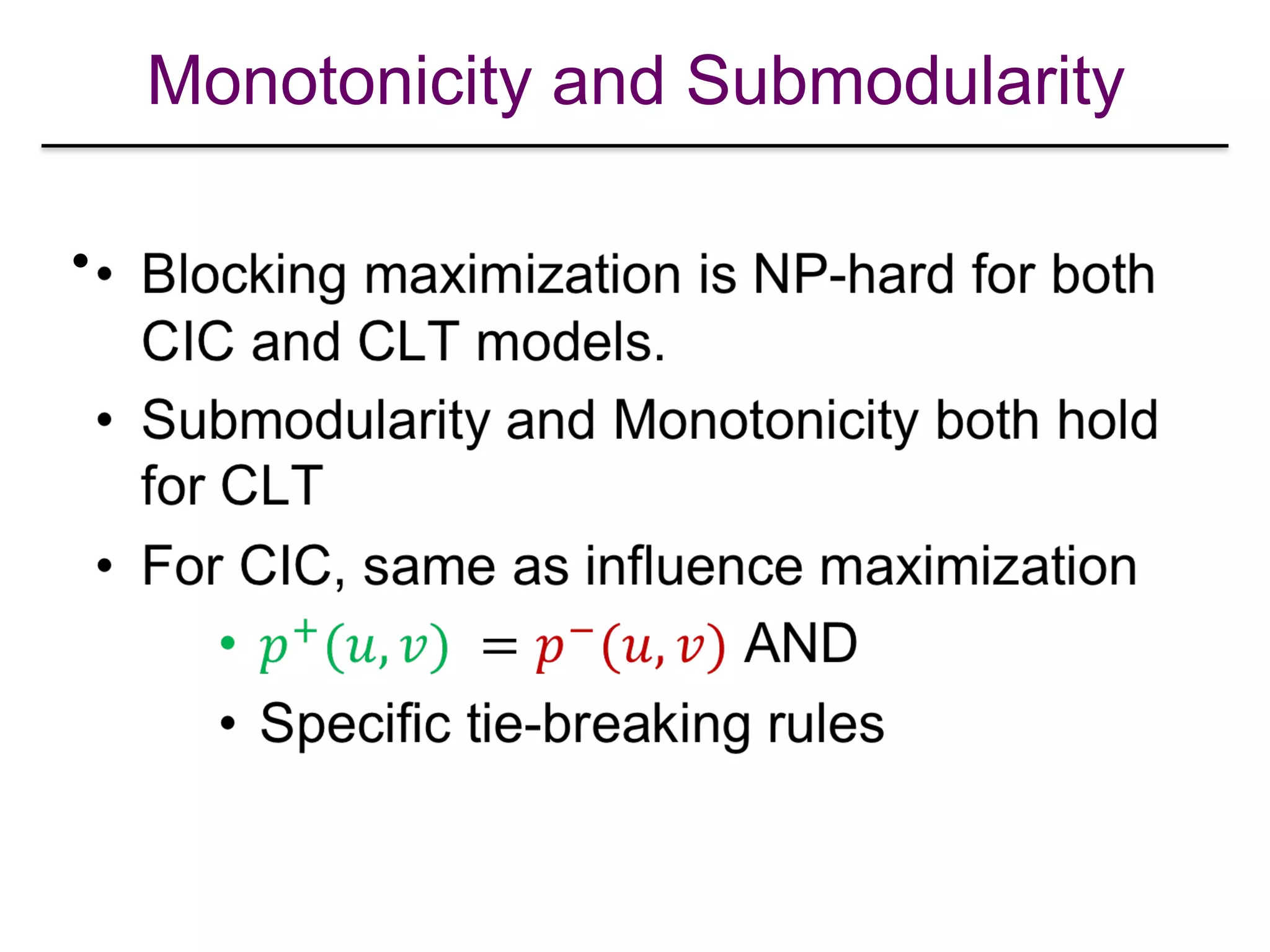
![Monotonicity and Submodularity
•
[Chen et al. “Information and Influence Propagation in Social Networks”, Morgan & Claypool 2013]](https://image.slidesharecdn.com/wsdm2018tutorial-180611122200/75/WSDM-2018-Tutorial-on-Influence-Maximization-in-Online-Social-Networks-139-2048.jpg)
![Influence Blocking Maximization
•
[Budak et al. Limiting the Spread of misinformation in Social Networks]
[He at al. “Influence Blocking Maximization in Social Networks under the Competitive Linear Threshold Model”, SDM 2012]](https://image.slidesharecdn.com/wsdm2018tutorial-180611122200/75/WSDM-2018-Tutorial-on-Influence-Maximization-in-Online-Social-Networks-140-2048.jpg)
![IC-N Model (Negative Opinion)
•
[Chen et al., “Influence Maximization in Social Networks When Negative Opinions May Emerge and Propagate”,
SDM 2011]](https://image.slidesharecdn.com/wsdm2018tutorial-180611122200/75/WSDM-2018-Tutorial-on-Influence-Maximization-in-Online-Social-Networks-142-2048.jpg)
![Weight-Proportional LT
•
[Borodin et al. Threshold models for competitive influence in social networks. WINE 2010.]](https://image.slidesharecdn.com/wsdm2018tutorial-180611122200/75/WSDM-2018-Tutorial-on-Influence-Maximization-in-Online-Social-Networks-143-2048.jpg)
![K-LT Model
•
[Lu et al. “The Bang for the Buck: Fair Competitive Viral Marketing from the Host Perspective”, KDD 2013]](https://image.slidesharecdn.com/wsdm2018tutorial-180611122200/75/WSDM-2018-Tutorial-on-Influence-Maximization-in-Online-Social-Networks-144-2048.jpg)
![Viral marketing as a service
[Lu et al. “The Bang for the Buck: Fair Competitive Viral Marketing from the Host Perspective”, KDD 2013]](https://image.slidesharecdn.com/wsdm2018tutorial-180611122200/75/WSDM-2018-Tutorial-on-Influence-Maximization-in-Online-Social-Networks-145-2048.jpg)
![Fair Allocation
•
[Lu et al. “The Bang for the Buck: Fair Competitive Viral Marketing from the Host Perspective”, KDD 2013]](https://image.slidesharecdn.com/wsdm2018tutorial-180611122200/75/WSDM-2018-Tutorial-on-Influence-Maximization-in-Online-Social-Networks-146-2048.jpg)

![Competition & Complementarity
• Any relationship is possible
– Compete (iPhone vs Nexus)
– Complement (iPhone & Apple Watch)
– Indifferent (iPhone & Umbrella)
• Classical economics concepts: Substitute &
complementary goods
• Item relationship may be asymmetric
• Item relationship may be to an arbitrary extent
[Lu et al. “From Competition to Complementarity: Comparative Influence Diffusion and Maximization”, KDD 2013]](https://image.slidesharecdn.com/wsdm2018tutorial-180611122200/75/WSDM-2018-Tutorial-on-Influence-Maximization-in-Online-Social-Networks-148-2048.jpg)
![Modeling Complementarity
•
[Narayanam et al. “Viral marketing for product cross-sell through social networks”, PKDD 2012]](https://image.slidesharecdn.com/wsdm2018tutorial-180611122200/75/WSDM-2018-Tutorial-on-Influence-Maximization-in-Online-Social-Networks-149-2048.jpg)
![Comparative Influence Cascade (Com-IC)
• Com-IC Model: A unified model
characterizing both competition and
complementarity to arbitrary degree
• Edge-level: influence/information
propagation
• Node-level: Decision-making controlled by
an automata (“global adoption
probabilities”)
[Lu et al. “From Competition to Complementarity: Comparative Influence Diffusion and Maximization”, KDD 2013]](https://image.slidesharecdn.com/wsdm2018tutorial-180611122200/75/WSDM-2018-Tutorial-on-Influence-Maximization-in-Online-Social-Networks-150-2048.jpg)
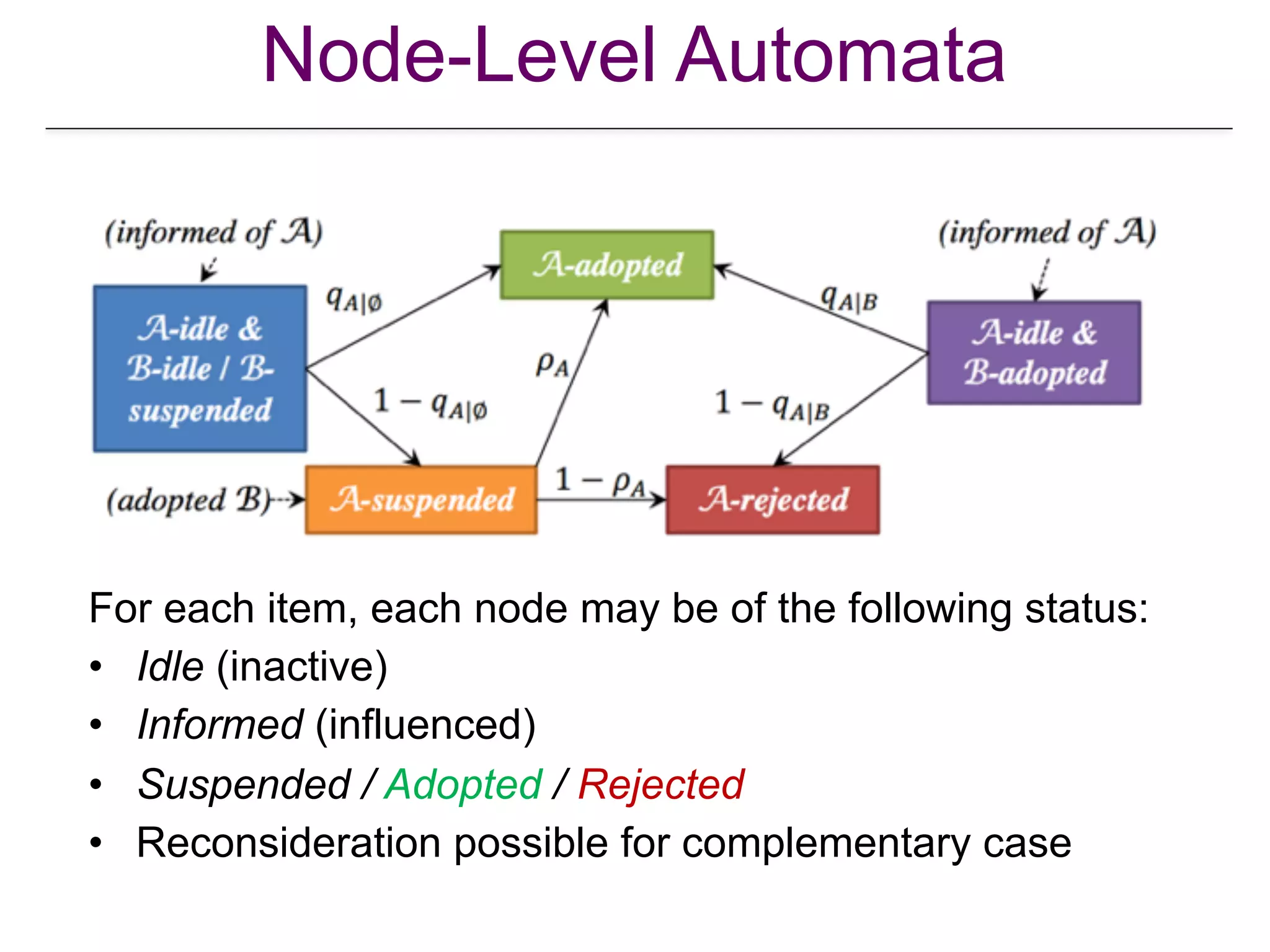
![Global Adoption Probabilities
•
[Lu et al. “From Competition to Complementarity: Comparative Influence Diffusion and Maximization”, KDD 2013]](https://image.slidesharecdn.com/wsdm2018tutorial-180611122200/75/WSDM-2018-Tutorial-on-Influence-Maximization-in-Online-Social-Networks-151-2048.jpg)
![Complementarity oriented
maximization objective
•
[Lu et al. “From Competition to Complementarity: Comparative Influence Diffusion and Maximization”, KDD 2013]](https://image.slidesharecdn.com/wsdm2018tutorial-180611122200/75/WSDM-2018-Tutorial-on-Influence-Maximization-in-Online-Social-Networks-153-2048.jpg)
![Generalized Reverse Sampling
•
[Lu et al. “From Competition to Complementarity: Comparative Influence Diffusion and Maximization”, KDD 2013]](https://image.slidesharecdn.com/wsdm2018tutorial-180611122200/75/WSDM-2018-Tutorial-on-Influence-Maximization-in-Online-Social-Networks-154-2048.jpg)
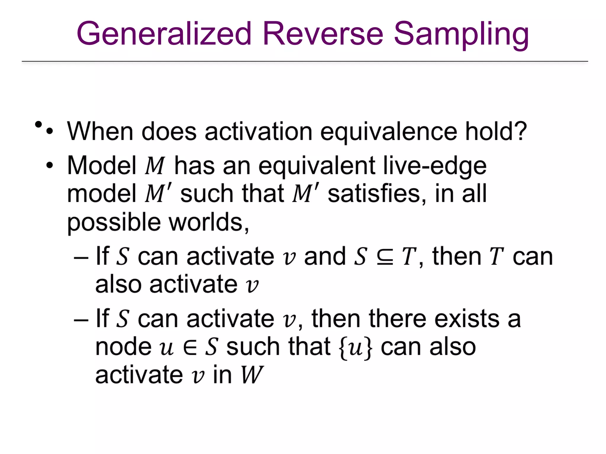
![Generalized Reverse Sampling
•
[Lu et al. “From Competition to Complementarity: Comparative Influence Diffusion and Maximization”, KDD 2013]](https://image.slidesharecdn.com/wsdm2018tutorial-180611122200/75/WSDM-2018-Tutorial-on-Influence-Maximization-in-Online-Social-Networks-155-2048.jpg)
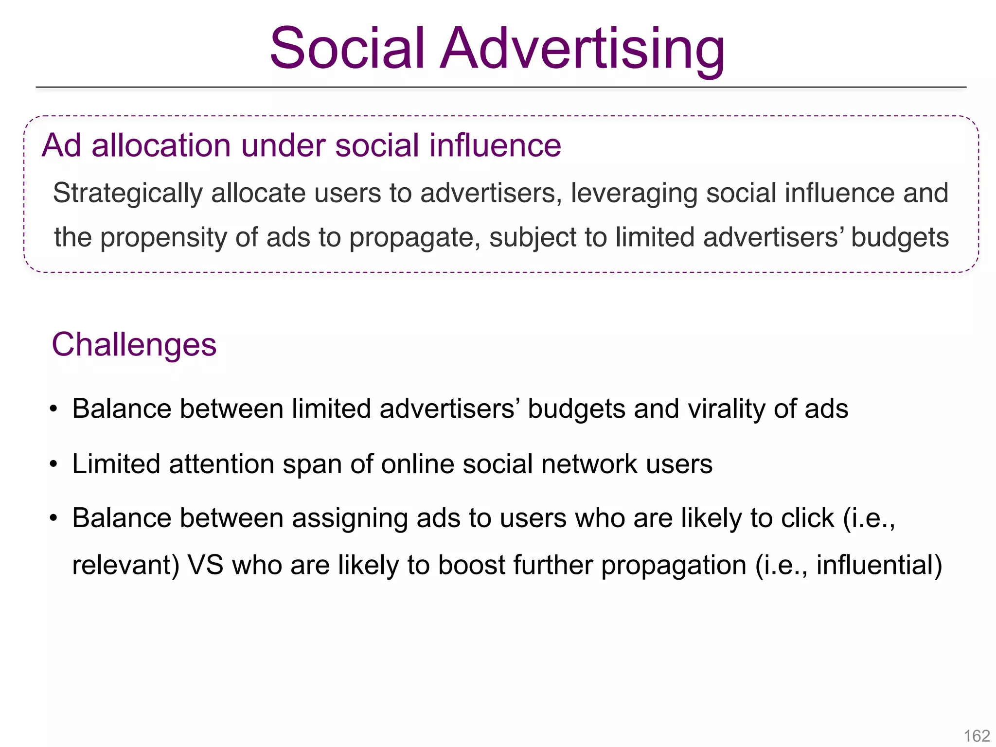
![• Balance between intrinsic relevance in the absence of social proof and
peer influence
• Ad-specific CTP for each user: δ(u,i)
• Probability that user u will click ad i in the absence of social proof
• TIC-CTP reduces to TIC model with pi
H,u = δ(u,i)
• When δ(u,i) = 1 for all u and i, TIC = TIC-CTP
v
u
wH
puw
puv
pHv
pHw
pHu
!163[Aslay et al., “Viral marketing meets social advertising: Ad allocation with minimum regret”, VLDB 2015]
Extending TIC model with Click-Through-Probabilities
Ad Relevance vs Social Influence](https://image.slidesharecdn.com/wsdm2018tutorial-180611122200/75/WSDM-2018-Tutorial-on-Influence-Maximization-in-Online-Social-Networks-163-2048.jpg)
![Budget and Regret
• Host:
• Owns directed social graph G = (V,E) and TIC-CTP model instance
• Sets user attention bound κu for each user u ∊ V
• Advertiser i:
• agrees to pay CPE(i) for each click up to his budget Bi
• total monetary value of the clicks πi(Si) = σi(Si) × cpe(i)
• Exp. revenue of the host from assigning seed set Si to ad i: min(πi(Si), Bi)
Host’s regret
!164
• πi(Si) < Bi : Lost revenue opportunity
• πi(Si) > Bi : Free service to the advertiser
[Aslay et al., “Viral marketing meets social advertising: Ad allocation with minimum regret”, VLDB 2015]](https://image.slidesharecdn.com/wsdm2018tutorial-180611122200/75/WSDM-2018-Tutorial-on-Influence-Maximization-in-Online-Social-Networks-164-2048.jpg)
![Budget and Regret
(Raw) Allocation Regret
• Regret of the host from allocating seed set Si to advertiser i:
Ri(Si) = |Bi − πi(Si) |
• Overall allocation regret:
R(S1, …, Sh) = Ri(Si)
Penalized Allocation Regret
• λ: penalty to discourage selecting large number of poor quality seeds
• Regret of the host with seed set size penalization
Ri(Si) = |Bi − πi(Si) | + λ × |Si|
!165
hX
i=1
[Aslay et al., “Viral marketing meets social advertising: Ad allocation with minimum regret”, VLDB 2015]](https://image.slidesharecdn.com/wsdm2018tutorial-180611122200/75/WSDM-2018-Tutorial-on-Influence-Maximization-in-Online-Social-Networks-165-2048.jpg)
![Regret Minimization
• Given
• a social graph G = (V,E)
• TIC-CTP propagation model
• h advertisers with budget Bi and cpe(i) for each advertiser i
• attention bound κu for each user u ∊ V
• penalty parameter λ ≥ 0
• Find a valid allocation S = (S1, …, Sh) that minimizes the overall regret of the
host from the allocation:
!166[Aslay et al., “Viral marketing meets social advertising: Ad allocation with minimum regret”, VLDB 2015]](https://image.slidesharecdn.com/wsdm2018tutorial-180611122200/75/WSDM-2018-Tutorial-on-Influence-Maximization-in-Online-Social-Networks-166-2048.jpg)
![• Regret-Minimization is NP-hard and is NP-hard to approximate
• Reduction from 3-PARTITION problem
• Regret function is neither monotone nor submodular
• Mon. decreasing and submodular for πi(Si) < Bi and πi(Si U {u}) < Bi
• Mon. increasing and submodular for πi(Si) > Bi and πi(Si U {u}) > Bi
• Neither monotone nor submodular for πi(Si) < Bi and πi(Si U {u}) > Bi
!167
Regret Minimization
Bi
πi(Si) πi(Si U {u})
[Aslay et al., “Viral marketing meets social advertising: Ad allocation with minimum regret”, VLDB 2015]](https://image.slidesharecdn.com/wsdm2018tutorial-180611122200/75/WSDM-2018-Tutorial-on-Influence-Maximization-in-Online-Social-Networks-167-2048.jpg)
![!168
• A greedy algorithm
• Select the (ad i, user u) pair that gives the max. reduction in regret at
each step, while respecting the attention constraints
• Stop the allocation to i when Ri(Si) starts to increase
• Approximation guarantees w.r.t. the total budget of all
advertisers:
• Theorem 2: for λ > 0, details omitted
• Theorem 3: for λ = 0: R(S) ≤
• Theorem 4: for λ = 0: R(S) ≤
#P-Hard
Regret Minimization
[Aslay et al., “Viral marketing meets social advertising: Ad allocation with minimum regret”, VLDB 2015]
1
3
·
hX
i=1
Bi
max
i2[h],u2V
cpe(i) · i({u})
Bi
·
hX
i=1
Bi](https://image.slidesharecdn.com/wsdm2018tutorial-180611122200/75/WSDM-2018-Tutorial-on-Influence-Maximization-in-Online-Social-Networks-168-2048.jpg)
![Two-Phase Iterative Regret Minimization (TIRM)
* Tang et al., “Influence maximization: Near-optimal time complexity meets practical efficiency”, SIGMOD 2014
TIM* cannot be used for minimizing the regret
① Does not handle CTPs
② Requires predefined seed set size s
!169
Scalable Regret Minimization
• Built on the Reverse Influence Sampling framework of TIM
• RR-sets sampling under TIC-CTP model: RRC-sets
• Iterative seed set size estimation
[Aslay et al., “Viral marketing meets social advertising: Ad allocation with minimum regret”, VLDB 2015]](https://image.slidesharecdn.com/wsdm2018tutorial-180611122200/75/WSDM-2018-Tutorial-on-Influence-Maximization-in-Online-Social-Networks-169-2048.jpg)
![(1) RR-sets sampling under TIC-CTP model: RRC-sets
• Sample a random RR set R for advertiser i
• Remove every node u in R with probability 1 – δ(u,i)
• Form “RRC-set” from the remaining nodes
Scalability compromised:
Requires at least 2 orders of magnitude bigger
sample size for CTP = 0.01.
Theorem 5: MG(u | S) in IC-CTP = δ(u) * MG(u | S) in IC
!170
Scalable Regret Minimization
[Aslay et al., “Viral marketing meets social advertising: Ad allocation with minimum regret”, VLDB 2015]](https://image.slidesharecdn.com/wsdm2018tutorial-180611122200/75/WSDM-2018-Tutorial-on-Influence-Maximization-in-Online-Social-Networks-170-2048.jpg)
![For each advertiser i:
• Start with a “safe” initial seed set size si
• Sample θi(si) RR sets required for si
• Update si based on current regret
• Revise θi(si), sample additional RR sets, revise estimates
(2) Iterative Seed Set Size Estimation
Estimation accuracy of TIRM Theorem 6
!171
Scalable Regret Minimization
[Aslay et al., “Viral marketing meets social advertising: Ad allocation with minimum regret”, VLDB 2015]](https://image.slidesharecdn.com/wsdm2018tutorial-180611122200/75/WSDM-2018-Tutorial-on-Influence-Maximization-in-Online-Social-Networks-171-2048.jpg)
![Ui(S) =
(
⇧i(Si) if ⇧i(Si) Bi
2Bi ⇧i(Si) otherwise.
• Define utility function from
``Approximable” Regret
[Tang and Yuan, “Optimizing ad allocation in social advertising”, CIKM 2016 ]
• Regret-Minimization is NP-hard and is NP-hard to approximate
• Reduction from 3-PARTITION problem
• Regret function is neither monotone nor submodular
Bi
πi(Si) πi(Si U {u})
[Aslay et al., VLDB 2015]](https://image.slidesharecdn.com/wsdm2018tutorial-180611122200/75/WSDM-2018-Tutorial-on-Influence-Maximization-in-Online-Social-Networks-172-2048.jpg)
![!173[Tang and Yuan, “Optimizing ad allocation in social advertising”, CIKM 2016 ]
• Constant approx. under the assumption maxv i({v}) < bBi/cpe(i)c
``Approximable” Regret
Minimize
hX
i=1
|Bi ⇧i(Si)|
hX
i=1
Ui(S)
Maximize Maximize (submodular)
hX
i=1
min(Bi, ⇧i(Si))
(1/4)-approximation (1/2)-approximation*
Partition matroid• User attention bound constraint
* Fisher, et al., "An analysis of approximations for maximizing submodular set functions II." Polyhedral Combinatorics 1978
Submodular maximization
subject to matroid constraint](https://image.slidesharecdn.com/wsdm2018tutorial-180611122200/75/WSDM-2018-Tutorial-on-Influence-Maximization-in-Online-Social-Networks-173-2048.jpg)
![Sponsored Social Advertising
!174
Advertiser
• Pays a fixed CPE to host for each
engagement up to his budget
• Gives free products / discount coupons to
seed users
[Chalermsook et al., “Social network monetization via sponsored viral marketing”, SIGMETRICS 2015]
ki
min(Bi, ⇧i(Si))
• No -approximation algorithm possible unless P = NPO(n1 ✏
)
• Unlimited advertiser budgets O(log n)-approximation
maximize
(S1,··· ,Sh)
X
i2[h]
min(Bi, ⇧i(Si))
subject to |Si| ki, 8i 2 [h]
Find an allocation S = (S1, …, Sh) maximizing the revenue of the host:](https://image.slidesharecdn.com/wsdm2018tutorial-180611122200/75/WSDM-2018-Tutorial-on-Influence-Maximization-in-Online-Social-Networks-174-2048.jpg)
![Incentivized Social Advertising
CPE Model with Seed User Incentives
!175
• Host
• Sells ad-engagements to advertisers
• Inserts promoted posts to feed of users in exchange for monetary incentives
• Seed users take a cut on the social advertising revenue
• Advertiser
• Pays a fixed CPE to host for each
engagement
• Pays monetary incentive to each seed
user engaging with his ad
• Total payment subject to his budget
[Aslay et al., “Revenue Maximization in Incentivized Social Advertising”, VLDB 2017]](https://image.slidesharecdn.com/wsdm2018tutorial-180611122200/75/WSDM-2018-Tutorial-on-Influence-Maximization-in-Online-Social-Networks-175-2048.jpg)
![• Given
• a social graph G = (V,E)
• TIC propagation model
• h advertisers with budget Bi and CPE(i) for each ad i
• seed user incentives ci(u) for each user u∈V and for each ad i
• Find an allocation S = (S1, …, Sh) maximizing the overall revenue of the
host:
!176
Incentivized Social Advertising
[Aslay et al., “Revenue Maximization in Incentivized Social Advertising”, VLDB 2017]](https://image.slidesharecdn.com/wsdm2018tutorial-180611122200/75/WSDM-2018-Tutorial-on-Influence-Maximization-in-Online-Social-Networks-176-2048.jpg)
![• Revenue-Maximization problem is NP-hard
• Restricted special case with h = 1:
• NP-Hard Submodular-Cost Submodular-Knapsack* (SCSK) problem
!177
*Iyer et al., “Submodular optimization with submodular cover and submodular knapsack constraints”, NIPS 2013.
Partition matroid
Submodular knapsack constraints
• Family 𝘊 of feasible solutions form an Independence System
• Two greedy approximation algorithms w.r.t. sensitivity to seed user
costs during the node selection
Incentivized Social Advertising
[Aslay et al., “Revenue Maximization in Incentivized Social Advertising”, VLDB 2017]](https://image.slidesharecdn.com/wsdm2018tutorial-180611122200/75/WSDM-2018-Tutorial-on-Influence-Maximization-in-Online-Social-Networks-177-2048.jpg)
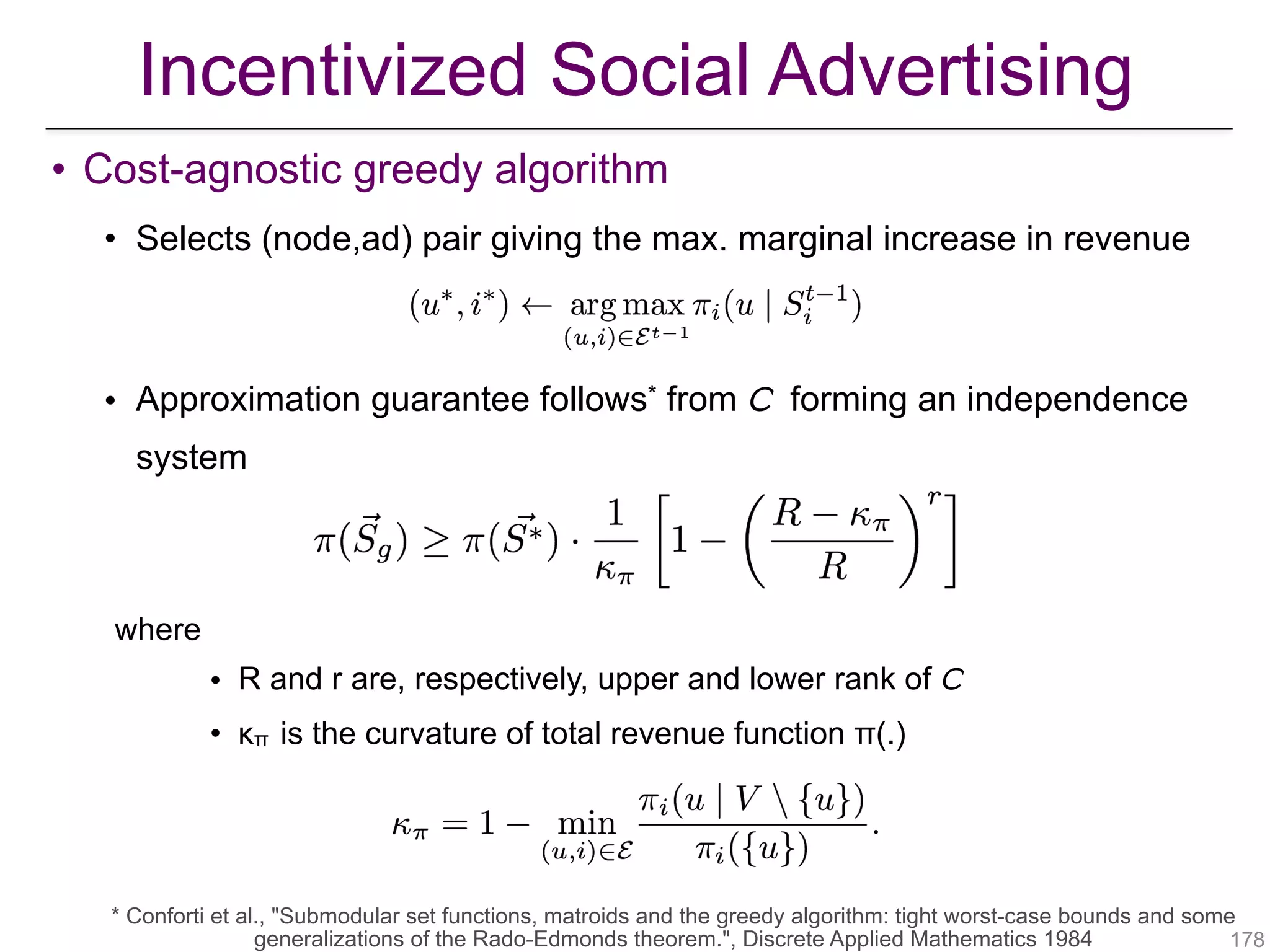
![• Cost-sensitive greedy algorithm
• Selects the (node,ad) pair giving the max. rate of marginal gain in
revenue per marginal gain in payment
• Approximation guarantee obtained
where
• ρmax and ρmin are, respectively, max. and min. singleton payments
• κρi is the curvature of ad i’s payment function ρi(.)
!179
Incentivized Social Advertising
[Aslay et al., “Revenue Maximization in Incentivized Social Advertising”, VLDB 2017]](https://image.slidesharecdn.com/wsdm2018tutorial-180611122200/75/WSDM-2018-Tutorial-on-Influence-Maximization-in-Online-Social-Networks-179-2048.jpg)
![Two-Phase Iterative Revenue Maximization
• Built on the Reverse Influence Sampling framework of TIRM*
• Latent seed set size estimation
!180
• Two-Phase Iterative Cost-Agnostic Revenue Maximization (TI-CARM)
• Two-Phase Iterative Cost-Sensitive Revenue Maximization (TI-CSRM)
Incentivized Social Advertising
[Aslay et al., “Revenue Maximization in Incentivized Social Advertising”, VLDB 2017]](https://image.slidesharecdn.com/wsdm2018tutorial-180611122200/75/WSDM-2018-Tutorial-on-Influence-Maximization-in-Online-Social-Networks-180-2048.jpg)
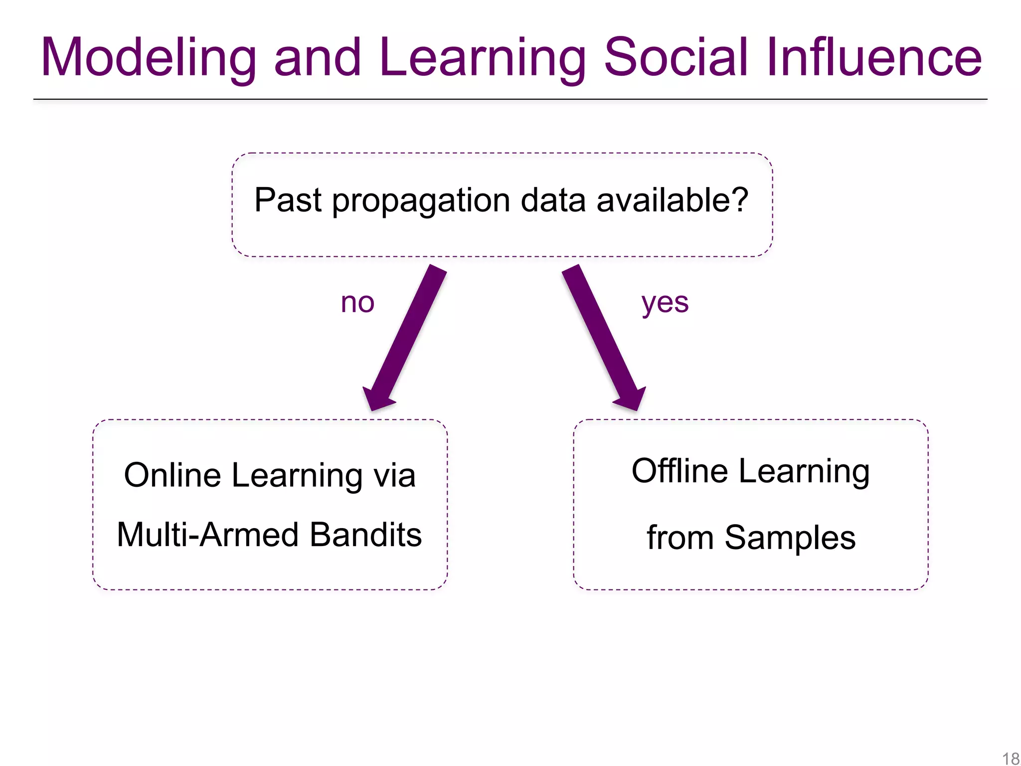
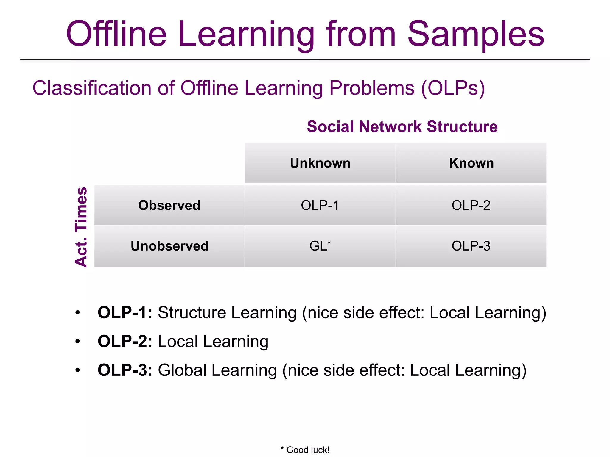
![OLP1: Network Unknown & Activation Times Observed
• Sample = {tc}c∈D where tc = [tc(u1), …, tc(un)] is activation times in cascade c
• tc(u) = ∞ for inactive u in cascade c
• If node v tends to get activated soon after node u in many different
cascades, then (u,v) is possibly an edge in unknown G
• Local Learning is a nice side affect of Structure Learning!
Structure Learning
Actual Network Learned Network
Local Learning
[Myers & Leskovec, "On the Convexity of Latent Social Network Inference", NIPS 2010]
[Gomez-Rodriguez, Leskovec, & Krause, "Inferring networks of diffusion and influence", KDD 2010]](https://image.slidesharecdn.com/wsdm2018tutorial-180611122200/75/WSDM-2018-Tutorial-on-Influence-Maximization-in-Online-Social-Networks-185-2048.jpg)
![OLP1: Network Unknown & Activation Times Observed
Structure Learning as a Convex Optimization Problem
• pvu = P(v activates u | v is active) Parameters of the
IC / SI / SIS / SIR model
• Likelihood function:
• Let denote the set of nodes in c activated before time tXc(t)
successful activations
failed activations
L(p; D) = ⇧c2D
✓
⇧
u:tc(u)<1
P(u activated at tc(u) | Xc(tc(u)))
◆
·
✓
⇧
u:tc(u)=1
P(u never active | Xc(t), 8t)
◆
[Myers & Leskovec, "On the Convexity of Latent Social Network Inference", NIPS 2010]](https://image.slidesharecdn.com/wsdm2018tutorial-180611122200/75/WSDM-2018-Tutorial-on-Influence-Maximization-in-Online-Social-Networks-186-2048.jpg)
![OLP1: Network Unknown & Activation Times Observed
Structure Learning as a Convex Optimization Problem
[Myers & Leskovec, "On the Convexity of Latent Social Network Inference", NIPS 2010]
• Assume probability of a successful activation decays with time
• Convexification:
• Convex program with n2 - n variables
• No guarantees wrt sample complexity!
P(u act. at tc(u) | Xc(tc(u))) = 1 ⇧
v:tc(v)tc(u)
[1 pvu · f(tc(u) tc(v))]
P(u never active | Xc(t), 8t) = ⇧
v:tc(v)<1
(1 pvu)
andc = 1 ⇧
v:tc(v)tc(u)
[1 pvu · f(tc(u) tc(v))] ✓vu = 1 pvu
• Maximize Minimizelog L(p, D) log L(✓, , D)](https://image.slidesharecdn.com/wsdm2018tutorial-180611122200/75/WSDM-2018-Tutorial-on-Influence-Maximization-in-Online-Social-Networks-187-2048.jpg)
![OLP1: Network Unknown & Activation Times Observed
[Netrapalli & Sanghavi, "Learning the graph of epidemic cascades", SIGMETRICS 2012]
Structure Learning as a Convex Optimization Problem
• Assume correlation decay instead (of time decay)
• Cascade from seed nodes do not travel far
• Average distance from a node to a seed is at most
• For any node u
X
v2Nin(u)
Avu < 1 ↵ P(tc(u) = t) (1 ↵)t 1
pinitand
1/↵
failed activations
successful activations
correlation decay
L(p; D) = ps
init(1 pinit)n s
·
✓
⇧
u:tc(u)=1
⇧
v:tc(v)<1
(1 pvu)
◆
· ⇧c2D
✓
⇧
u:tc(u)<1
1 ⇧
v:tc(v)tc(u)
(1 pvu)
◆
• Likelihood function with s seeds](https://image.slidesharecdn.com/wsdm2018tutorial-180611122200/75/WSDM-2018-Tutorial-on-Influence-Maximization-in-Online-Social-Networks-188-2048.jpg)
![OLP1: Network Unknown & Activation Times Observed
[Netrapalli & Sanghavi, "Learning the graph of epidemic cascades", SIGMETRICS 2012]
Structure Learning as a Convex Optimization Problem
• Maximize Minimizelog L(p, D) log L(✓, D)
• Convexification: ✓vu = 1 pvu
• Decouples into n convex programs, i.e., one per node
• Activation attempts are independent in IC / SI / SIS / SIR models
• Sample complexity results as a function of pinit and
• LB for per node neighborhood recovery and learning
• LB for whole graph recovery and learning
↵](https://image.slidesharecdn.com/wsdm2018tutorial-180611122200/75/WSDM-2018-Tutorial-on-Influence-Maximization-in-Online-Social-Networks-189-2048.jpg)
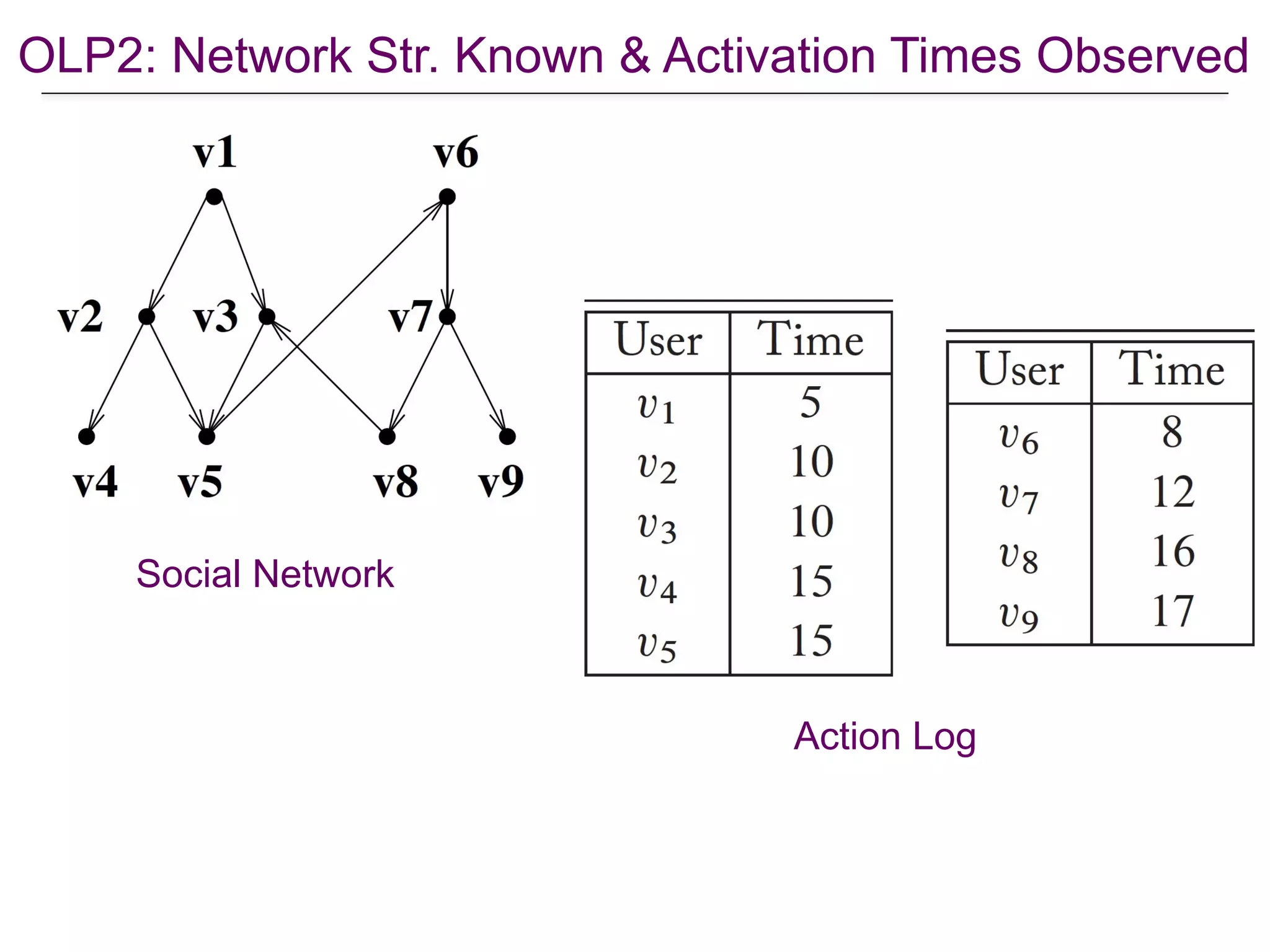
![OLP2: Network Str. Known & Activation Times Observed
• Sample = {(Xc(0), …, Xc(T))}c∈D where Xc(t) are the nodes activated at
time t in cascade c. Define Yc(t’) = ∪t∈[1:t’] Xc(t).
• Likelihood of a single cascade c
[Saito et al., “Prediction of Information Diffusion Probabilities for Independent Cascade Model”, KES 2008]
• Use Expectation Maximization to solve L(p,D) for p
• Computationally very expensive, not scalable!
L(p, c) =
0
@
T 1Y
t=0
Y
u2Xc(t+1)
(1
Y
v2Nin(u)Yc(t)
(1 pvu))
1
A
·
0
@
T 1Y
t=0
Y
u2Xc(t)
Y
v2Nout(u)Yc(t)
(1 pvu)
1
A
success
failure
• Likelihood of D: L(p, D) =
Y
c2D
L(p, c)](https://image.slidesharecdn.com/wsdm2018tutorial-180611122200/75/WSDM-2018-Tutorial-on-Influence-Maximization-in-Online-Social-Networks-191-2048.jpg)
![OLP2: Network Str. Known & Activation Times Observed
• MLE procedure of Saito et al.
• Learning limited to IC model
• Assumes influence weights remain constant over time
• Accuracy depends on how well the activation times are discretized
[Goyal, Bonchi, & Lakshmanan, "Learning influence probabilities in social networks", WSDM 2010]
• A frequentist modeling approach for learning by Goyal et al.
• Active neighbor v of u remains contagious in [t, t + 𝛕(u,v)], has constant
probability puv in this interval and 0 outside
• Can Learn IC, LT, and General Threshold models
• Models are able to predict when a user will perform an action!
• Minimum possible number of scans of the propagation log with
chronologically sorted data](https://image.slidesharecdn.com/wsdm2018tutorial-180611122200/75/WSDM-2018-Tutorial-on-Influence-Maximization-in-Online-Social-Networks-192-2048.jpg)
![OLP3: Network Str. Known & Activation Times Unobserved
• Sample = {(Sc, Xc)}c∈D where Sc are the seeds of cascade c and Xc are the
complete set of active nodes in cascade c
• Interpret IC / LT influence functions as coverage functions
• Each node u reachable from seed set S is covered with certain weight au
• au : conditional probability that node u would be influenced by S
• Expected influence spread = the weighted sum of coverage weights:
[Du et al., “Influence Function Learning in Information Diffusion Networks", ICML 2014]
(S) =
X
u2[s2S Xs
au
• Sampled cascades (Sc,Xc): instantiations of random reachability matrix
• MLE for random basis approximations
• Polynomial sample complexity results wrt the desired accuracy level!](https://image.slidesharecdn.com/wsdm2018tutorial-180611122200/75/WSDM-2018-Tutorial-on-Influence-Maximization-in-Online-Social-Networks-193-2048.jpg)
![OLP3: Network Str. Known & Activation Times Unobserved
* Valiant, “A theory of the learnable”, Communications of the ACM, 1984
• PAC learning*: Probably Approximately Correct learning
• A formal framework of learning with accuracy and confidence
guarantees!
• PAC learning of IC / LT influence functions
• Sample complexity wrt the desired accuracy level and confidence
• Also solves OLP2 with learnability guarantees!
[Narasimhan, Parkes, & Singer, "Learnability of Influence in Networks", NIPS 2015]
Influence functions are PAC learnable!
• Influence function F : 2V → [0,1]n
• For a given seed set S
F(S) = [F1(S), …, Fn(S)]
• Fu(S) is the probability of u being influence during any time step](https://image.slidesharecdn.com/wsdm2018tutorial-180611122200/75/WSDM-2018-Tutorial-on-Influence-Maximization-in-Online-Social-Networks-194-2048.jpg)
![OLP3: Network Str. Known & Activation Times Unobserved
• FG: class of all influence functions over G for different parametrization
• The seeds of cascades are drawn iid from a distribution
• Measuring error from expected loss over random draws of S and X:
error[F] = ES,X[loss(X, F(S))]
[Narasimhan, Parkes, & Singer, "Learnability of Influence in Networks", NIPS 2015]
PAC learnability of influence functions
µ
discrepancy between predicted and observed
• Goal: learn a function FD ∈ FG that best explains the sample D:
probably
P(error[FD] inf
F 2FG
error[F] ✏) 1
approximately](https://image.slidesharecdn.com/wsdm2018tutorial-180611122200/75/WSDM-2018-Tutorial-on-Influence-Maximization-in-Online-Social-Networks-195-2048.jpg)
![OLP3: Network Str. Known & Activation Times Unobserved
• LT influence functions as multi-layer
neural network classifiers
• Linear threshold activations
• Local influence as a two-layer NN
• Extension to multiple-layer NN by
replicating the output layer
[Narasimhan, Parkes, & Singer, "Learnability of Influence in Networks", NIPS 2015]
LT model
• Learnability guarantees follow from neural-network classifiers
• Finite VC dimension of NNs implies PAC-learnability](https://image.slidesharecdn.com/wsdm2018tutorial-180611122200/75/WSDM-2018-Tutorial-on-Influence-Maximization-in-Online-Social-Networks-196-2048.jpg)
![OLP3: Network Str. Known & Activation Times Unobserved
[Narasimhan, Parkes, & Singer, "Learnability of Influence in Networks", NIPS 2015]
LT model
• Exact solution gives zero training error on the sample
• Due to deterministic nature of LT functions
• Is computationally very hard to solve exactly
• Equivalent to learning a recurrent neural network
• Approximations possible by
• Replacing threshold activations with sigmoidal activations
• Using continuous surrogate loss instead of binary loss function
• Exact polynomial time learning possible when there is also the
activation times!](https://image.slidesharecdn.com/wsdm2018tutorial-180611122200/75/WSDM-2018-Tutorial-on-Influence-Maximization-in-Online-Social-Networks-197-2048.jpg)
![• IC influence function as expectation over a random draw of a subgraph A
• Let Fp denote the global IC function for parametrization p
[Narasimhan, Parkes, & Singer, "Learnability of Influence in Networks", NIPS 2015]
IC model
• Define the global log-likelihood for cascade c = (Sc, Xc):
Fp
u (S) =
X
A✓E
Y
(a,b)2A
pab ·
Y
(a,b)62A
(1 pab) · 1(S reaches u in A)
L(Sc
, Xc
, p) =
nX
u=1
1(u2Xc) log Fp
u (S) + (1 1(u2Xc)) log(1 Fp
u (S))
success failure
OLP3: Network Str. Known & Activation Times Unobserved](https://image.slidesharecdn.com/wsdm2018tutorial-180611122200/75/WSDM-2018-Tutorial-on-Influence-Maximization-in-Online-Social-Networks-198-2048.jpg)
![[Narasimhan, Parkes, & Singer, "Learnability of Influence in Networks", NIPS 2015]
IC model
max
p2[ ,1 ]m
X
c2D
L(Sc
, Xc
, p)
• Learnability follows from standard uniform convergence arguments
• Construct an ∊-cover of the space
• Use Lipschitzness to translate this to ∊-cover of IC function class
• Uniform convergence implies PAC learnability
[ , 1 ]
• MLE of the overall log-likelihood to obtain p
kp p0
k ✏ |Fp
u (S) Fp0
u (S)| ✏
• Use Lipschitzness (i.e., bounded-derivative) property of IC function
class to obtain Fp from p with guarantees
OLP3: Network Str. Known & Activation Times Unobserved](https://image.slidesharecdn.com/wsdm2018tutorial-180611122200/75/WSDM-2018-Tutorial-on-Influence-Maximization-in-Online-Social-Networks-199-2048.jpg)
![• Sample = {(Sc, Xc)}c∈D where Sc are the seeds of cascade c and Xc are
the ``complete” set of active nodes in cascade c
• What if the cascades are not ``complete”?
• When using Twitter API to collect cascades
• Solution: Adjust the distributional assumptions of the PAC learning
framework!
• The seeds of cascades are drawn iid from a distribution
• Partially observed cascades Xc are drawn from a distribution over
the random activations of Sc
[He, Xu, Kempe, & Liu., “Learning Influence Functions from Incomplete Observations”, NIPS 2016]
over seeds
OLP3: Network Str. Known & Activation Times Unobserved](https://image.slidesharecdn.com/wsdm2018tutorial-180611122200/75/WSDM-2018-Tutorial-on-Influence-Maximization-in-Online-Social-Networks-200-2048.jpg)
![• PAC learning with two distributional assumptions
• The seeds of cascades are drawn iid from a distribution
• Partially observed cascades Xc are drawn from a distribution over
the random activations of Sc
• Extension of Narasimhan et al.’s methods are not efficient with the
additional distributional assumptions (on Xc)
• PAC learning of random reachability matrix
• Learning model-free coverage functions as defined by Du et al.*
• Polynomial sample complexity for solving (only) OLP3
[He, Xu, Kempe, & Liu., “Learning Influence Functions from Incomplete Observations”, NIPS 2016]
* Du et al., “Influence Function Learning in Information Diffusion Networks", ICML 2014
OLP3: Network Str. Known & Activation Times Unobserved](https://image.slidesharecdn.com/wsdm2018tutorial-180611122200/75/WSDM-2018-Tutorial-on-Influence-Maximization-in-Online-Social-Networks-201-2048.jpg)
![• Influence functions are PAC learnable from samples but the
influence maximization from samples is intractable
• Requires exponentially many samples
• No algorithm can provide constant-factor approximation
guarantee using polynomially many samples
How about directly solving the influence maximization problem
directly from a given sample??
Solving IM from Samples
[Balkanski, Rubinstein, and Singer. “The limitations of optimization from samples”, STOC 2017]](https://image.slidesharecdn.com/wsdm2018tutorial-180611122200/75/WSDM-2018-Tutorial-on-Influence-Maximization-in-Online-Social-Networks-202-2048.jpg)
![Solving IM from Samples
[Goyal, Bonchi, & Lakshmanan, "A data-based approach to social influence maximization", VLDB 2011]
A frequentist mining approach](https://image.slidesharecdn.com/wsdm2018tutorial-180611122200/75/WSDM-2018-Tutorial-on-Influence-Maximization-in-Online-Social-Networks-203-2048.jpg)
![• Instead of learning the probabilities and simulating propagations, use
available propagations to estimate the expected spread
Solving IM from Samples
[Goyal, Bonchi, & Lakshmanan, "A data-based approach to social influence maximization", VLDB 2011]
A frequentist mining approach
(S) =
X
u2V
E[path(S, u)] =
X
u2V
P[path(S, u) = 1]
• We cannot estimate directly P[path(S,u)] from the sample
• Sparsity issues where S is effectively the seed of a cascade
• Take a u-centric perspective instead:
• Each time u performs an action, distribute the ``influence credit”
• Resulting credit distribution model is submodular
• Find the top-k seed from the sample via greedy algorithm
• Very efficient but no formal guarantees wrt the ``real optimal seed set”](https://image.slidesharecdn.com/wsdm2018tutorial-180611122200/75/WSDM-2018-Tutorial-on-Influence-Maximization-in-Online-Social-Networks-204-2048.jpg)
![• Leverage strong community structures of social networks
• Identify a set of users who are influentials but whose communities
have little overlap
• Define a tolerance parameter α for the allowed community overlap
• Greedy algorithm to find top-k seeds wrt allowed overlap
A formal but constrained approach
P
Sc⇠µ,8c2D
[E[f(S)] ↵ max
T ✓V
f(T)] 1
• First formal way to optimize IC functions from samples!
[Balkanski, Immorlica, & Singer, “The Importance of Communities for Learning to Influence", NIPS 2017]
Solving IM from Samples](https://image.slidesharecdn.com/wsdm2018tutorial-180611122200/75/WSDM-2018-Tutorial-on-Influence-Maximization-in-Online-Social-Networks-205-2048.jpg)
![Multi-Armed Bandits (MAB)
•
[Audibert et al. “Introduction to Bandits: Algorithm and Theory”, ICML 2011]](https://image.slidesharecdn.com/wsdm2018tutorial-180611122200/75/WSDM-2018-Tutorial-on-Influence-Maximization-in-Online-Social-Networks-209-2048.jpg)
![Exploration & Exploitation
•
[Audibert et al. “Introduction to Bandits: Algorithm and Theory”, ICML 2011]](https://image.slidesharecdn.com/wsdm2018tutorial-180611122200/75/WSDM-2018-Tutorial-on-Influence-Maximization-in-Online-Social-Networks-210-2048.jpg)
![UCB Strategy
•
[Audibert et al. “Introduction to Bandits: Algorithm and Theory”, ICML 2011]](https://image.slidesharecdn.com/wsdm2018tutorial-180611122200/75/WSDM-2018-Tutorial-on-Influence-Maximization-in-Online-Social-Networks-211-2048.jpg)

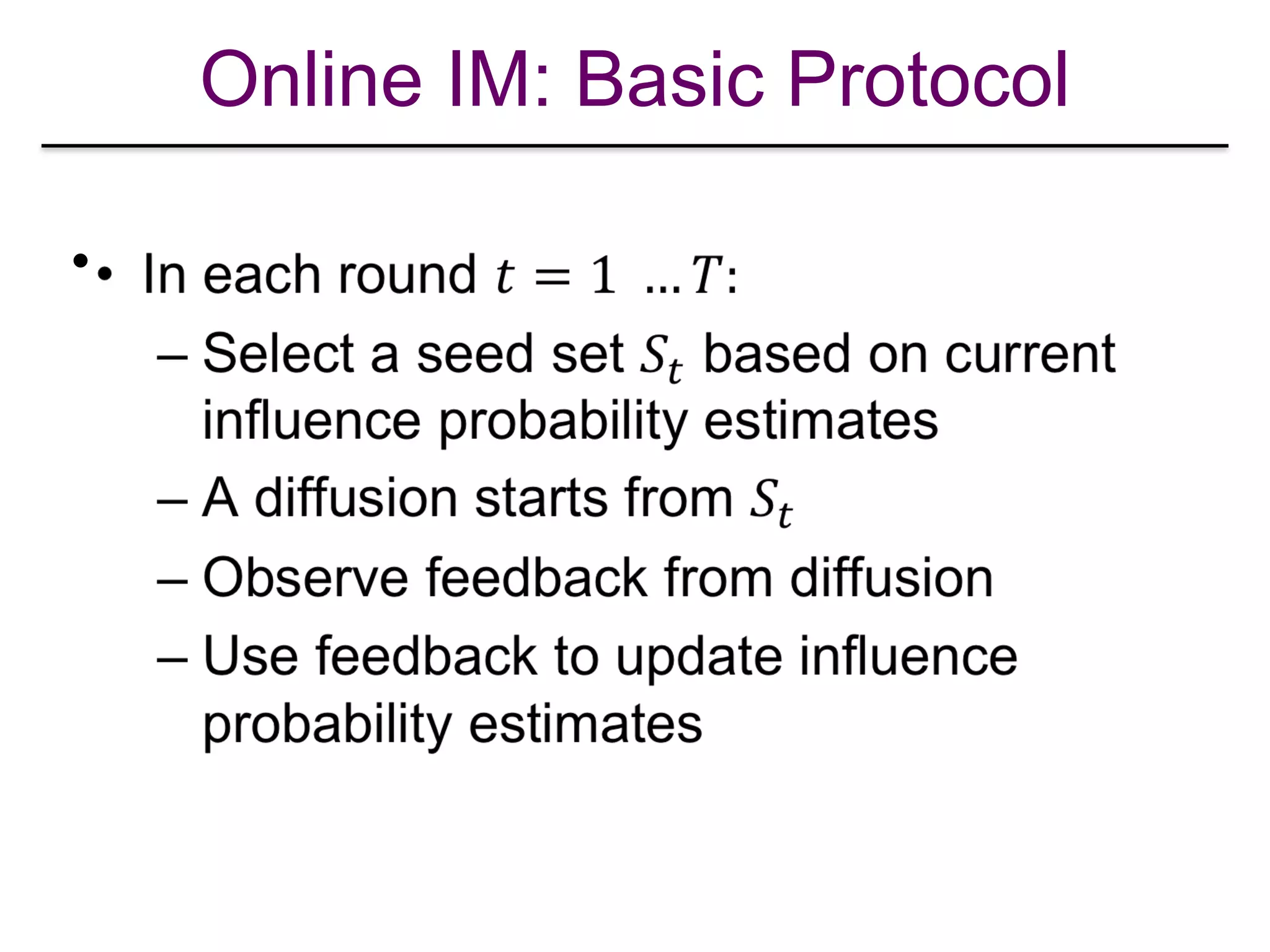
![Explore-Exploit in Online IM
•
[Lei et al. “Online Influence Maximization”, KDD 2015]](https://image.slidesharecdn.com/wsdm2018tutorial-180611122200/75/WSDM-2018-Tutorial-on-Influence-Maximization-in-Online-Social-Networks-218-2048.jpg)
![Explore-Exploit in Online IM
•
[Lei et al. “Online Influence Maximization”, KDD 2015]](https://image.slidesharecdn.com/wsdm2018tutorial-180611122200/75/WSDM-2018-Tutorial-on-Influence-Maximization-in-Online-Social-Networks-219-2048.jpg)

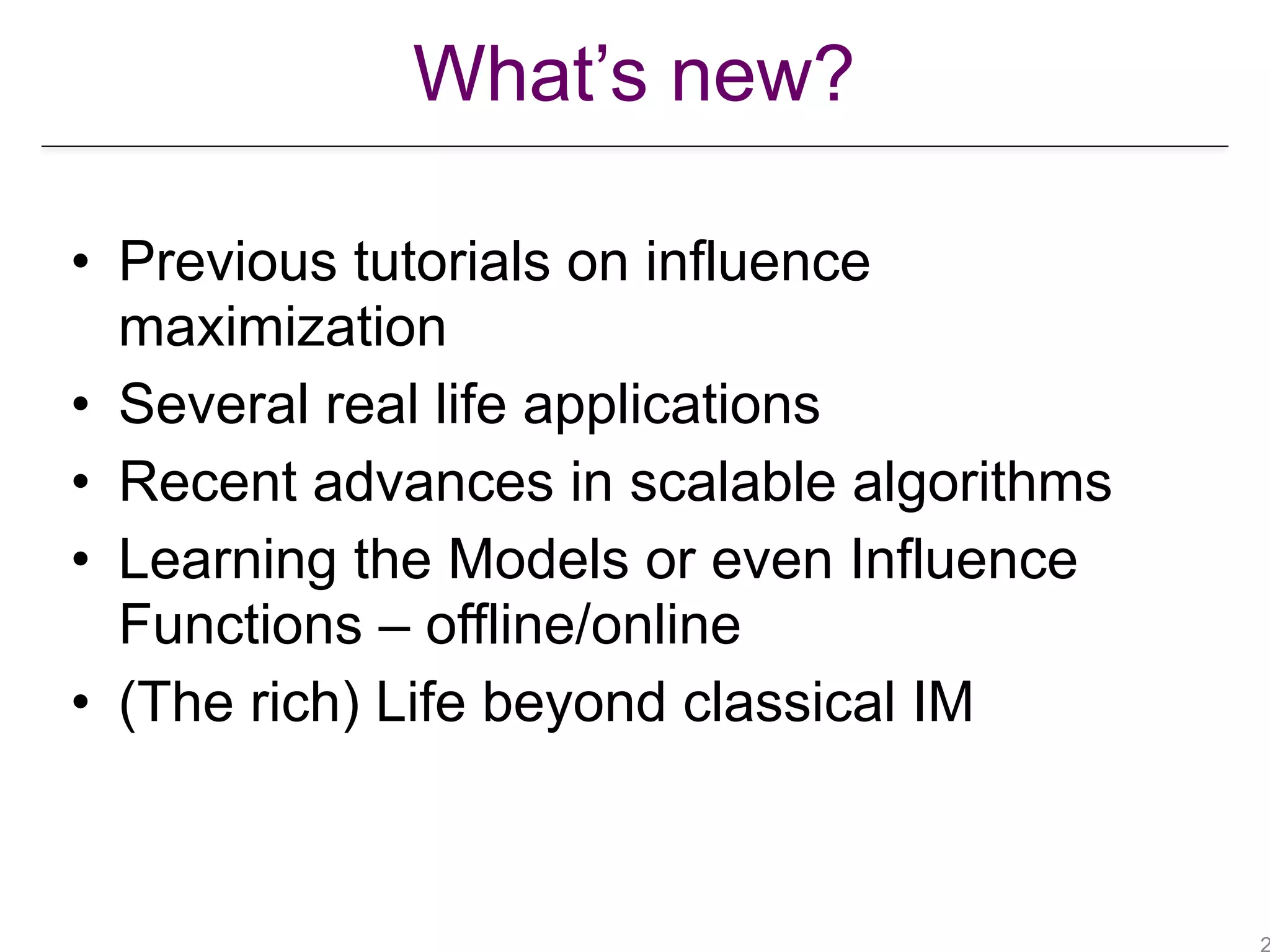
The document presents a tutorial on influence maximization in online social networks, covering its definitions, importance, theoretical foundations, and real-life applications like viral marketing and political mobilization. It discusses various algorithms and models for scalable approximation, including heuristics for optimizing influence spread and challenges in computational complexity. The tutorial outlines different parts, including offline and online model learning, multiple campaigns, and social advertising.